Current Fluctuations in One Dimensional Diffusive Systems with a Step Initial Density Profile

Abstract

We show how to apply the macroscopic fluctuation theory (MFT) of Bertini, De Sole, Gabrielli, Jona-Lasinio, and Landim to study the current fluctuations of diffusive systems with a step initial condition. We argue that one has to distinguish between two ways of averaging (the annealed and the quenched cases) depending on whether we let the initial condition fluctuate or not. Although the initial condition is not a steady state, the distribution of the current satisfies a symmetry very reminiscent of the fluctuation theorem. We show how the equations of the MFT can be solved in the case of non-interacting particles. The symmetry of these equations can be used to deduce the distribution of the current for several other models, from its knowledge DG for the symmetric simple exclusion process. In the range where the integrated current $Q_{t}\sim\sqrt{t}$, we show that the non-Gaussian decay $\exp[-Q_{t}^{3}/t]$ of the distribution of $Q_{t}$ is generic.  
 
keywords: current fluctuations, step initial condition, fluctuation theorem

This work is dedicated to our master and friend Joel Lebowitz on the occasion of the 100th Statistical Mechanics Meeting held at Rutgers University in December 2008.

I Introduction

The study of the fluctuations of currents of energy or of particles is central in the theory of non-equilibrium systems. Over the last decade, the macrosopic fluctuation theory (MFT), a theory of diffusive systems maintained in a non-equilibrium steady state by contact with two heat baths or two reservoirs of particles, has been developed BDGJLY ; BDGJLX . This theory was first implemented to give a framework to calculate the large deviation functional of density profiles in non-equilibrium steady states BDGJL1 ; BDGJL2 ; BGLeb ; BGLan ; KTL ; Touch . It was then understood that it could also be used to predict the distribution of the current through non-equilibrium diffusive systems BD ; BDGJL5 ; BD2005 ; BDGJL6 ; BD2007 ; ADLW .

The macroscopic fluctuation theory gives a large scale description of lattice models such as the symmetric simple exclusion process (SSEP) or the Kipnis Marchioro Presutti model KMP ; HG ; HG2 ; Imparato . At the microcopic level, several properties of these models can be obtained using numerical HG ; HG2 ; GKP , perturbative DDR ; WR , or exact approaches HRS1 , such as the matrix method DLS1 ; DLS2 ; ED or the Bethe ansatz ADLW ; PM1 ; PM2 . Whenever the comparison has been possible, it is remarkable that a perfect agreement has been found between the results (on the large deviations of the density profile DLS1 ; DLS2 ; ED or on the probability distribution of the current HG ; HG2 ; DDR ) obtained by these microscopic approaches and the predictions of the macroscopic fluctuation theory BDGJL2 ; BGLan ; BD . Moreover the MFT led to the prediction of rather surprising properties of diffusive systems, such as the possibility of phase transitions BD2005 ; BDGJL6 ; BD2007 in the large deviation function of the current, or the universality of the cumulants of the current on the ring geometry ADLW . So far the MFT has only been used on systems at equilibrium, or in non-equilibrium steady states.

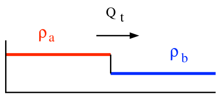
Figure 1: The step initial condition with a density $\rho_{a}$ at the left of the origin and $\rho_{b}$ at the right of the origin

In a recent work DG , we considered the fluctuations of the integrated current $Q_{t}$ through the origin of the SSEP, starting with a non steady state initial condition : a step in the density profile at the origin with density $\rho_{a}$ on the negative axis and density $\rho_{b}$ on the positive axis, as shown in figure 1. The SSEP is one of the simplest lattice gas models, and has been extensively studied in the theory of non-equilibrium systems HS ; Liggett2 ; derrida2007 . The distribution of the integrated current $Q_{t}$, for the SSEP, is related to the time decay of constrained one dimensional Ising models Spohn-spin . In the SSEP, particles diffuse on the lattice with nearest neighbor jumps and a hard core interaction which enforces that there is never more than one particle on each site (in practice, the configuration at time $t$ is specified by a binary variable $\tau_{i}(t)=\{1$ or $0\}$ on each lattice site, which indicates whether site $i$ is occupied or empty; the dynamics is such that these occupation numbers are exchanged at rate 1 between every pair of neighboring sites on the lattice). Using the Bethe ansatz and several identities proved recently by Tracy and Widom TW1 ; TW2 ; TW3 for exclusion processes on the line, we were able to show DG that the generating function of the total flux $Q_{t}$ of particles through the origin during a long time $t$ takes the form

$$\left\langle e^{\lambda Q_{t}}\right\rangle\asymp e^{\sqrt{t}\mu(\lambda,\rho_{a},\rho_{b})}\,,$$ (1)

with $\mu(\lambda,\rho_{a},\rho_{b})$ given by

$$\mu(\lambda,\rho_{a},\rho_{b})={1\over{\pi}}\int_{-\infty}^{\infty}dk\log\left[1+\omega e^{-k^{2}}\right]\,,$$ (2)

and where $\omega$ is a function of $\rho_{a},\rho_{b}$ and $\lambda$

$$\omega=\rho_{a}(e^{\lambda}-1)+\rho_{b}(e^{-\lambda}-1)+\rho_{a}\rho_{b}(e^{\lambda}-1)(e^{-\lambda}-1)\,.$$ (3)

Beyond the fact that that $\mu$ is a function of the single parameter $\omega$, which was proved in DG , one can see from (1,2,3) that

1. All the cumulants of $Q_{t}$ grow like $\sqrt{t}$.

2. $\mu(\lambda,\rho_{a},\rho_{b})$ satisfies a symmetry very reminiscent of the fluctuation theorem ECM ; GC ; Kurchan ; LS ; Maes ; Harris-S :

   $$\mu\Big{(}\lambda,\rho_{a},\rho_{b}\Big{)}=\mu\left(-\lambda+\log{\rho_{b}\over 1-\rho_{b}}-\log{\rho_{a}\over 1-\rho_{a}},\rho_{a},\rho_{b}\right)$$ (4)

   (this is because $\omega$ in (3) is left unchanged by this symmetry).

3. For technical reasons in the way that (2) was derived in DG , we had to impose the condition that $|\omega|<\sqrt{2/\pi}$. If one assumes that the range of validity of (2) extends to all $\omega>-1$, one gets that $\mu\simeq{4\over 3\pi}(\log\omega)^{3/2}$ for large $\omega$, which would imply that for large $q$

   $${\rm Probability}\left({Q_{t}\over\sqrt{t}}\simeq q\right)\asymp\exp\left[-{\pi^{2}\over 12}\;q^{3}\;\sqrt{t}\right]=\exp\left[-{\pi^{2}\over 12}\;{Q_{t}^{3}\over t}\right]\,.$$ (5)

The goal of the present work is to see how the above results (1-5), obtained for the SSEP with the step initial condition of figure 1, can be understood from the point of view of the MFT and how they can be extended to more general diffusive systems.

When the dynamics is stochastic, the integrated current $Q_{t}$ through the origin depends both on the history (i.e. on all the updates between time $0$ and time $t$) and on the initial condition (which, for the SSEP, is drawn according to a Bernoulli measure of mean $\rho_{a}$ on the negative axis ($i\leq 0$) and $\rho_{b}$ on the positive axis ($i\geq 1$)). Very much like in the theory of disordered systems, where one can distinguish between an annealed average (where the partition function is averaged over all the realizations of the disorder) and a quenched average (where the partition function is calculated for a typical realization of the disorder), one can define here two expressions of $\mu(\lambda)$  :

• the annealed case where, as in the derivation of (1-3) in DG , one averages $e^{\lambda Q_{t}}$ both on the history and on the initial condition

  $$\mu_{\rm annnealed}(\lambda)=\lim_{t\to\infty}{1\over\sqrt{t}}\log\left[\left\langle e^{\lambda Q_{t}}\right\rangle_{\rm history,\ initial\;condition}\right];$$ (6)

  It turns out that the initial conditions which dominate the average are atypical as shown in figure 2.

• the quenched case, where one averages $e^{\lambda Q_{t}}$ only on the history for a typical initial condition

  $$\mu_{\rm quenched}(\lambda)=\lim_{t\to\infty}{1\over\sqrt{t}}\left\langle\ \log\left[\left\langle e^{\lambda Q_{t}}\right\rangle_{\rm history}\right]\ \right\rangle_{\rm initial\;condition}\,.$$ (7)

The difference between these two averages, and their influence on the distribution of the current, has already been studied for the totally asymmetric exclusion process (TASEP) using the microscopic dynamics PS2 .

In section II, we formulate the calculation of both $\mu_{\rm annealed}$ and $\mu_{\rm quenched}$ in the framework of the MFT. In section III, we see that $\mu_{\rm annealed}$ satisfies the symmetry (4) for general diffusive systems, and for general non-steady state initial conditions. No such symmetry seems to hold in the quenched case. In section IV, we consider the case of non-interacting random walkers, where both $\mu_{\rm annealed}$ and $\mu_{\rm quenched}$ can be determined exactly. In section V, we show that, for the SSEP, the single-parameter dependence (3) of $\mu_{\rm annealed}$ can be understood from a remarkable invariance of the MFT. In section VI, we obtain bounds on the decay of the distribution of $Q_{t}$ which shows that (5) is generic for a broader class of diffusive systems.

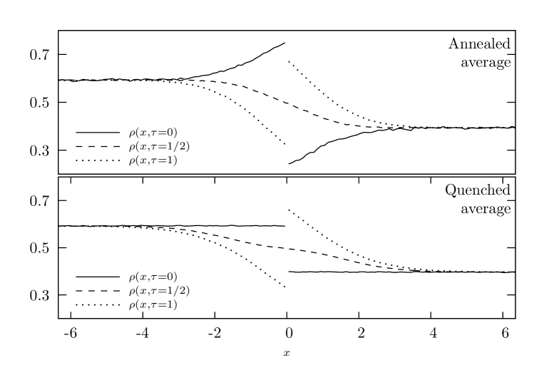
Figure 2: Average rescaled density $\rho(x,\tau)$ (see (14)) for the SSEP, in the annealed and quenched cases, when $\lambda=1.5$, $\rho_{a}=0.6$ and $\rho_{b}=0.4$. While the initial profile is a step function in the quenched case, it deviates from it in the annealed case.

II The annealed and the quenched averages

In this section we show how the macroscopic fluctuation theory BDGJLY ; BDGJLX can be used to calculate the generating function of the integrated current $Q_{t}$ when the initial condition is a step density profile. The theory is in principle valid for arbitrary diffusive systems with one conserved quantity, such as the number of particles or the energy. Here, for simplicity, we consider the case of a one dimensional lattice gas where a configuration is characterized by the numbers $n_{i}$ of particles on each site $i$.

Imagine first that this one dimensional system has a finite length $L$, and that it is in contact, at its two ends, with two reservoirs of particles at density $\rho_{a}$ and $\rho_{b}$. In this finite geometry, the system’s stochastic evolution reaches a steady state, where the flux $Q_{t}$ of particles during a long $t$ has a certain average $\langle Q_{t}\rangle$ and a certain variance $\langle Q_{t}^{2}\rangle_{c}=\langle Q_{t}^{2}\rangle-\langle Q_{t}\rangle^{2}$. Close to equilibrium, i.e. when the densities of the two reservoirs are close ($\rho_{a}\simeq\rho_{b}\simeq r$ with $\rho_{a}-\rho_{b}\ll r$), and for a large system size $L$, one expects BD ; derrida2007 that

$$\lim_{t\to\infty}{\langle Q_{t}\rangle\over t}\simeq{D(r)\over L}(\rho_{a}-\rho_{b})$$ (8)

and

$$\lim_{t\to\infty}{\langle Q_{t}^{2}\rangle_{c}\over t}\simeq{\sigma(r)\over L}\,,$$ (9)

where $D(r)$ and $\sigma(r)$ are two functions which characterize the transport of particles through this diffusive system.

At equilibrium (for $\rho_{a}=\rho_{b}=r$), the weights of all microscopic configurations are given by the Boltzmann weights. For large $L$, if one introduces a rescaled position $0<x=i/L<1$, the probability of observing a given density profile $\rho(x)$, when the two reservoirs are at the same density $r$, satisfies derrida2007 ; BDGJLZ

$${\rm Pro_{eq.}}(\rho(x))\asymp\exp[-L{\cal F}_{\rm eq.}(\rho(x))]\,,$$

where the large deviation function ${\cal F}_{\rm eq.}$ is given by

$${\cal F}_{\rm eq.}(\rho(x))=\int_{0}^{1}\Big{[}f(\rho(x))-f(r)-(\rho(x)-r)f^{\prime}(r)\Big{]}dx\,,$$ (10)

and $f(r)$ is the free energy per site of the equilibrium system at density $r$ (defined as $f(r)=-\lim_{L\to\infty}(\log Z(Lr,L))/L$) for $Z(N,L)$ the partition function of the system with $N$ particles on $L$ sites). One can show HS ; derrida2007 that the fluctuation dissipation theorem, which is satisfied at equilibrium, implies that

$$f^{\prime\prime}(r)={2D(r)\over\sigma(r)}{\,.}$$ (11)

For a diffusive system on a one dimensional lattice of $L$ sites, in contact with two reservoirs at densities $\rho_{a}$ and $\rho_{b}$, the average density $\langle n_{i}(t)\rangle$ near position $i$ and time $t$, and the total flux of particles $Q_{i}(t)$ through position $i$ between times $0$ and $t$, are expected to follow diffusive scaling laws. For large $L$, and for times of order $L^{2}$, they take the form

$$\langle n_{i}(t)\rangle=\rho\left({i\over L},{t\over L^{2}}\right)\qquad{\rm and}\qquad Q_{i}(t)=L\;q\left({i\over L},{t\over L^{2}}\right)\;.$$

From the large deviation hydrodynamics theory KOV ; HS ; KL ; BD2007 ; derrida2007 , the probability of observing a certain density profile $\rho\left(x,\tau\right)$ and current profile $j\left(x,\tau\right)\equiv\partial q(x,\tau)/\partial\tau$ over the rescaled time interval $0<\tau<t/L^{2}$ is expressed as

$${\rm Pro}\Big{(}\{\rho(x,\tau),j(x,\tau)\}\Big{)}\asymp\exp\left[-L\int_{0}^{t/L^{2}}d\tau\int_{0}^{1}dx\ {\left[j(x,\tau)+D({\rho(x,\tau})){\partial{\rho(x,\tau)}\over\partial x}\right]^{2}\over 2\sigma(\rho(x,\tau))}\right]{\,,}$$ (12)

where $D(\rho)$ and $\sigma(\rho)$ are defined as in (8,9). Expression (12) simply means that, locally, Fick’s law ($j=-D(\rho)\rho^{\prime}$) is satisfied everywhere up to Gaussian current fluctuations of variance $\sigma(\rho)$. The conservation of the number of particles,
$n_{i}(t)-n_{i}(0)=Q_{i-1}(t)-Q_{i}(t)$, becomes a conservation law on the rescaled density and current profiles :

$${\partial\rho\over\partial\tau}=-{\partial j\over\partial x}\,.$$ (13)

For a non-steady state initial condition, as in figure 1, the system size is infinite. If one observes the fluctuations of the current over a long time $t$, one can introduce a characteristic length $\sqrt{t}$. The average density $\langle n_{i}(t^{\prime})\rangle$ near site $i$ and the integrated current $Q_{i}(t^{\prime})$ between times $0$ and $t^{\prime}<t$ then become scaling functions of the form

$$\langle n_{i}(t^{\prime})\rangle=\rho\left({i\over\sqrt{t}},{t^{\prime}\over t}\right)\qquad{\rm and}\qquad Q_{i}(t^{\prime})=\sqrt{t}\;q\left({i\over\sqrt{t}},{t^{\prime}\over t}\right)\;\,,$$ (14)

and the probability of observing such rescaled density and current profiles is given by

$${\rm Pro}\Big{(}\{\rho(x,\tau),j(x,\tau)\}\Big{)}\asymp\exp\left[-\sqrt{t}\int_{0}^{1}d\tau\int_{-\infty}^{\infty}dx\ {\left[j(x,\tau)+D({\rho(x,\tau})){\partial{\rho(x,\tau)}\over\partial x}\right]^{2}\over 2\sigma(\rho(x,\tau))}\right]\,.$$ (15)

The integrated current $Q_{t}$ through the origin during time $t$ can then be written as

$$Q_{t}=\sum_{i\geq 1}n_{i}(t)-n_{i}(0)\simeq\sqrt{t}\int_{0}^{\infty}dx\ [\rho(x,1)-\rho(x,0)]\,.$$ (16)

Moreover, when the initial condition is a local equilibrium configuration at density $\rho_{a}$ on the negative axis and density $\rho_{b}$ on the positive axis, as in figure 1, the probability ${\rm Pro_{\rm initial}}$ of the initial profile $\rho(x,0)$ is given by

$${\rm Pro_{\rm initial}}(\rho(x,0))\asymp\exp\left[-\sqrt{t}\;{\cal F}_{\rm init.}(\rho(x,0))\right]\,,$$ (17)

where (10,11)

$${\cal F}_{\rm init.}(\rho(x,0)) = \int_{-\infty}^{\infty}\Big{[}f(\rho(x,0))-f(r(x))-(\rho(x,0)-r(x))f^{\prime}(r(x))\Big{]}dx$$ (18)

$$= \int dx\int_{r(x)}^{\rho(x,0)}dz\ (\rho(x,0)-z){2D(z)\over\sigma(z)}\,,$$ (19)

and $r(x)$ is the step density profile

$$r(x)=(1-\theta(x))\rho_{a}+\theta(x)\rho_{b}$$ (20)

($\theta(x)$ is the Heaviside function).
 
The annealed case

Therefore (6, 15,16, 18) lead to the following expression for $\mu_{\rm annnealed}$ :

$$\mu_{\rm annnealed}(\lambda)=\max_{\rho(x,\tau),j(x,\tau)}\left\{-{\cal F}_{\rm init.}(\rho(x,0))+\lambda\int_{0}^{\infty}dx\;[\rho(x,1)-\rho(x,0)]-\int_{0}^{1}d\tau\int_{-\infty}^{\infty}dx\;{\left[j(x,\tau)+D({\rho(x,\tau})){\partial\rho(x,\tau)\over\partial x}\right]^{2}\over 2\sigma(\rho(x,\tau))}\right\}$$ (21)

Finding the optimal $\rho(x,\tau)$ and $j(x,\tau)$ in (21) has to be done carefully because they are related by the conservation law (13)

As shown in Appendix A (see also BDGJL2 ; KTL ), one can replace the variational form (21) by another variational form :

$$\mu_{\rm annnealed}(\lambda)=\max_{\rho(x,\tau),H(x,\tau)}\left\{-{\cal F}_{\rm init.}(\rho(x,0))+\lambda\int_{0}^{\infty}dx\;[\rho(x,1)-\rho(x,0)]\right.$$

$$\left.-\int_{0}^{1}d\tau\int_{-\infty}^{\infty}dx\left[H(x,\tau){\partial\rho(x,\tau)\over\partial\tau}+D(\rho(x,\tau)){\partial H(x,\tau)\over\partial x}{\partial\rho(x,\tau)\over\partial x}-{\sigma(\rho(x,\tau))\over 2}\left({\partial H(x,\tau)\over\partial x}\right)^{2}\right]\right\}\,,$$ (22)

where $\rho(x,\tau)$ and $H(x,\tau)$ are independent. The optimal $\rho(x,\tau)$ and $H(x,\tau)$ in (22) satisfy

$${\partial\rho(x,\tau)\over\partial\tau} = {\partial\over\partial x}\left[D(\rho(x,\tau)){\partial\rho(x,\tau)\over\partial x}\right]-{\partial\over\partial x}\left[\sigma(\rho(x,\tau)){\partial H(x,\tau)\over\partial x}\right]\,,$$ (23)

$${\partial H(x,\tau)\over\partial\tau} = -D(\rho(x,\tau)){\partial^{2}H(x,\tau)\over\partial x^{2}}-{\sigma^{\prime}(\rho(x,\tau))\over 2}\left({\partial H(x,\tau)\over\partial x}\right)^{2}\,,$$ (24)

with the boundary conditions

$$H(x,1) = \lambda\theta(x)\,,$$ (25)

$$H(x,0) = \lambda\theta(x)+2\int_{r(x)}^{\rho(x,0)}{D(\rho)\over\sigma(\rho)}d\rho\,,$$ (26)

where we have used (11) and (18).

Thus in annealed case one can use either (21) or (22-26) to obtain $\mu_{\rm annnealed}(\lambda)$. Using the fact that $\rho(x,\tau)$ satisfies (23) and that $\rho(x,\tau)$ and $H(x,\tau)$ have limiting values ($\rho_{a},\rho_{b}$) and ($0,\lambda$) as $x\to\pm\infty$, one can simplify (22) to get

$$\mu_{\rm annnealed}(\lambda)=-{\cal F}_{\rm init.}(\rho(x,0))+\lambda\int_{0}^{\infty}dx[\rho(x,1)-\rho(x,0)]-\int_{0}^{1}d\tau\int_{-\infty}^{\infty}dx{\sigma(\rho(x,\tau))\over 2}\left({\partial{H(x,\tau)}\over\partial x}\right)^{2}$$ (27)

The quenched case

In the quenched case, the main difference is that $\rho(x,0)$ is no longer allowed to fluctuate. Therefore the boundary condition (26) at $\tau=0$ is replaced by

$$\rho(x,0)=r(x)\,,$$ (28)

and (21) becomes

$$\mu_{\rm quenched}(\lambda)=\max_{\rho(x,\tau),j(x,\tau)}\left\{\lambda\int_{0}^{\infty}dx\;[\rho(x,1)-\rho(x,0)]-\int_{0}^{1}d\tau\int_{-\infty}^{\infty}dx\;{\left[j(x,\tau)+D(\rho(x,\tau)){\partial\rho(x,\tau)\over\partial x}\right]^{2}\over 2\sigma(\rho(x,\tau))}\right\}{\,,}$$ (29)

with the $\max$ taken over all the profiles satisfying (13) and (28). In terms of the field $H$, one gets

$$\mu_{\rm quenched}(\lambda)=\lambda\int_{0}^{\infty}dx[\rho(x,1)-\rho(x,0)]-\int_{0}^{1}d\tau\int_{-\infty}^{\infty}dx{\sigma(\rho(x,\tau)\over 2}\left({\partial{H(x,\tau)}\over\partial x}\right)^{2}\,,$$ (30)

with $\rho$ and $H$ satisfying (23-25) but with (28 ) instead of (26).  
 
 
 
 Remark : From the expressions (21,29) and (19),

$${\cal F}_{\rm init}(\rho(x,0))=\int dx\int_{r(x)}^{\rho(x,0)}dz\ (\rho(x,0)-z){2D(z)\over\sigma(z)}\,,$$

one can see that the case where $D(\rho)=1$ and $\sigma(\rho)$ is a quadratic function BGLeb ; Imparato of $\rho$,

$$D(\rho)=1\ \ \ \ ;\ \ \ \ \sigma(\rho)=2A\rho(B-\rho)\,,$$ (31)

can be easily related to the SSEP, for which (see BD )

$$D(\rho)=1\ \ \ \ ;\ \ \ \ \sigma(\rho)=2\rho(1-\rho)\,.$$ (32)

In fact, if one makes the change of variable

$$\rho\to B\rho\ \ \ \ ;\ \ \ \ j\to Bj$$

one gets for the choice (31) that, both in the annealed and in the quenched case,

$$\mu(\lambda,\rho_{a},\rho_{b})={1\over A}\mu_{SSEP}\left(AB\lambda,{\rho_{a}\over B},{\rho_{b}\over B}\right)\,.$$ (33)

In the annealed case, where the exact expression of the SSEP is available (1,2,3), one gets

$$\mu_{\rm annealed}(\lambda,\rho_{a},\rho_{b})={1\over A{\pi}}\int_{-\infty}^{\infty}dk\log\left[1+\omega e^{-k^{2}}\right]\,,$$ (34)

where

$$\omega={\rho_{a}(e^{AB\lambda}-1)\over B}+{\rho_{b}(e^{-AB\lambda}-1)\over B}+{\rho_{a}\rho_{b}(e^{AB\lambda}-1)(e^{-AB\lambda}-1)\over B^{2}}\,.$$ (35)

In the limit $A=B^{-1}\to 0$, this gives $\mu_{\rm annealed}$ when $\sigma=2\rho$, i.e. in the case of non-interacting particles (49) that we will discuss in section IV. Assuming that (34,35) remain valid for non-physical values of $A$ and $B$, one would get $\mu_{\rm annealed}$, without any further calculation, for the Kipnis Marchioro Presutti model KMP ; HG ; HG2 ; Imparato where $\sigma=4\rho^{2}$ (in the limit $B\to 0,A\to-2$).

III The time reversal symmetry

In this section we are going to see that the symmetry (4) can be extended to more general diffusive systems. To do so, let us consider the difference ${\cal F}_{\rm init.}(\rho(x,1))-{\cal F}_{\rm init.}(\rho(x,0))$. Using (18), one has

$${\cal F}_{\rm init.}(\rho(x,1))-{\cal F}_{\rm init.}(\rho(x,0))=\int_{-\infty}^{\infty}\Big{[}f(\rho(x,1))-f(\rho(x,0))-(\rho(x,1)-\rho(x,0))f^{\prime}(r(x))\Big{]}dx\,,$$

which can be rewritten as

$${\cal F}_{\rm init.}(\rho(x,1))-{\cal F}_{\rm init.}(\rho(x,0))=\int_{0}^{1}d\tau\int_{-\infty}^{\infty}dxf^{\prime}(\rho(x,\tau)){\partial\rho(x,\tau)\over d\tau}-\int_{-\infty}^{\infty}(\rho(x,1)-\rho(x,0))f^{\prime}(r(x))dx\,.$$

Then, using (13), an integration by parts, and (11), one gets

$${\cal F}_{\rm init.}(\rho(x,1))-{\cal F}_{\rm init.}(\rho(x,0))= \int_{0}^{1}d\tau\int_{-\infty}^{\infty}dxf^{\prime\prime}(\rho(x,\tau)){\partial\rho(x,\tau)\over\partial x}j(x,\tau)-\int_{-\infty}^{\infty}(\rho(x,1)-\rho(x,0))f^{\prime}(r(x))dx$$

$$= \int_{0}^{1}d\tau\int_{-\infty}^{\infty}dx{2D(\rho(x,\tau))\over\sigma(\rho(x,\tau))}{\partial\rho(x,\tau)\over\partial x}j(x,\tau)-\int_{-\infty}^{\infty}(\rho(x,1)-\rho(x,0))f^{\prime}(r(x))dx\,.$$

This allows one to rewrite the last term in (21) as

$$\iint d\tau dx\;{\left[j+D\partial_{x}\rho\right]^{2}\over 2\sigma}={{\cal F}_{\rm init.}(\rho(x,1))-{\cal F}_{\rm init.}(\rho(x,0))\over 2}+\int_{-\infty}^{\infty}(\rho(x,1)-\rho(x,0)){f^{\prime}(r(x))\over 2}dx+\iint d\tau dx\;{j^{2}+(D\partial_{x}\rho)^{2}\over 2\sigma}$$ (36)

and therefore (21) becomes

$$\mu_{\rm annnealed}(\lambda)=\max_{\rho(x,\tau),j(x,\tau)}\left\{-{{\cal F}_{\rm init.}(\rho(x,1))+{\cal F}_{\rm init.}(\rho(x,0))\over 2}+\int_{-\infty}^{\infty}dx\;[\rho(x,1)-\rho(x,0)]\left[\lambda\theta(x)-{f^{\prime}(r(x))\over 2}\right]\right.$$

$$\left.-\int_{0}^{1}d\tau\int_{-\infty}^{\infty}dx\;{j(x,\tau)^{2}+\left(D(\rho(x,\tau))\partial_{x}\rho(x,\tau)\right)^{2}\over 2\sigma(\rho(x,\tau))}\right\}\,.$$ (37)

For the step initial density profile (20), one has (11)

$$f^{\prime}(r(x))=f^{\prime}(\rho_{a})-\theta(x)\int_{\rho_{b}}^{\rho_{a}}{2D(\rho)\over\sigma(\rho)}d\rho\,.$$

One can then see in (37) that the initial time and the final time play symmetric roles : if one replaces $\{\rho(x,\tau),j(x,\tau)\}$ by $\{\rho(x,1-\tau),-j(x,1-\tau)\}$, (37) is left unchanged provided that $\lambda\to-\lambda-\int_{\rho_{b}}^{\rho_{a}}{2D(\rho)\over\sigma(\rho)}d\rho$. (one has to use that, from the conservation of the total number of particles, $\int_{-\infty}^{\infty}[\rho(x,1)-\rho(x,0)]dx=0$). Therefore $\mu_{\rm annealed}$ satisfies

$$\mu_{\rm annealed}\big{(}\lambda\big{)}=\mu_{\rm annealed}\Big{(}-\lambda-\int_{\rho_{b}}^{\rho_{a}}{2D(\rho)\over\sigma(\rho)}d\rho\Big{)}\,.$$ (38)

This is a generalization of (4) (for the SSEP (32), $D(\rho)=1$ and $\sigma(\rho)=2\rho(1-\rho)$, and (38) reduces to (4)) and therefore shows that a version derrida2007 of the fluctuation theorem ECM ; GC ; Kurchan ; LS ; Maes ; Harris-S holds for general diffusive systems with the step initial condition considered here. Although this initial condition is neither an equilibrium state, nor a non-equilibrium steady state, the time reversal symmetry (38) holds. We think that this is because, in the annealed case, the initial condition is in local equilibrium.

One can repeat the same transformations in the quenched case. Due to the absence of ${\cal F}_{\rm init.}(\rho(x,0))$ in (29), one ends up with an expression where $\rho(x,1)$ and $\rho(x,0)$ do not play symmetric roles, so that $\mu_{\rm quenched}$ does not seem to satisfy any kind of time reversal symmetry.  
 
Remark : By the same reasoning, one can show that the symmetry (38) holds for initial conditions more general than the step initial profile. One can consider at $t=0$ an initial density profile

$$r(x)=(1-v(x))\rho_{a}+v(x)\rho_{b}\,,$$ (39)

where $v(x)$ is no longer a step as in (20) but could be a more general sigmoid function with $v(-\infty)=0$ and $v(\infty)=1$. One can also replace the measure of the integrated current (16) at the origin by its weighted average over space in a region around the origin :

$$Q_{t}=\sqrt{t}\int_{-\infty}^{\infty}dx\;w(x)[\rho(x,1)-\rho(x,0)]\,,$$

where $w(x)$ is another sigmoid function. Then following exactly the same steps as in the derivation of (37) one gets

$$\mu_{\rm annnealed}(\lambda)=\max_{\rho(x,\tau),j(x,\tau)}\left\{-{{\cal F}_{\rm init.}(\rho(x,1))+{\cal F}_{\rm init.}(\rho(x,0))\over 2}+\int_{-\infty}^{\infty}dx\;[\rho(x,1)-\rho(x,0)]\left[\lambda w(x)+\int_{r(x)}^{\rho_{a}}{D(\rho)\over\sigma(\rho)}d\rho\right]\right.$$

$$\left.-\int_{0}^{1}d\tau\int_{-\infty}^{\infty}dx\;{j(x,\tau)^{2}+(D(\rho(x,\tau))\partial_{x}\rho(x,\tau))^{2}\over 2\sigma(\rho(x,\tau))}\right\}\,,\;\,$$

from which one can see that the time reversal symmetry (38) remains valid if $v(x)$ and $w(x)$ are related by

$$w(x)=\left[\int_{r(x)}^{\rho_{a}}{D(\rho)\over\sigma(\rho)}d\rho\right]/\left[\int_{\rho_{b}}^{\rho_{a}}{D(\rho)\over\sigma(\rho)}d\rho\right]\,.$$ (40)

Remark : No time reversal symmetry seems to hold in the quenched case. However, if an additional symmetry (the particle-hole symmetry) holds, one can relate $\mu_{\rm annealed}$ and $\mu_{\rm quenched}$. In Appendix B, we show that, if $D(\rho)$ and $\sigma(\rho)$ satisfy

$$\left\{\begin{array}[]{lll}D(\rho)&=&D(2\bar{\rho}-\rho)\\ \sigma(\rho)&=&\sigma(2\bar{\rho}-\rho)\end{array}\right.\,,$$ (41)

then the optimal profile $\rho^{\rm(a)}(x,\tau)$ for the annealed variational problem (21) when $\rho_{a}=\rho_{b}=\bar{\rho}$ is such that

$$\rho^{\rm(a)}(x,\tau)=2\bar{\rho}-\rho^{\rm(a)}(x,1-\tau)\ .$$ (42)

This implies in particular that $\rho^{\rm(a)}(x,\tau=1/2)=\bar{\rho}$ and allows one to relate the optimal annealed (21) and quenched (29) profiles (see Appendix B), leading to

$$\mu_{\rm quenched}(\lambda,\rho_{a}=\rho_{b}=\bar{\rho})={1\over\sqrt{2}}\mu_{\rm annealed}(\lambda,\rho_{a}=\rho_{b}=\bar{\rho})\,.$$ (43)

For the SSEP (32) the particle-hole symmetry (41) is satisfied, and therefore (43) holds, for $\bar{\rho}=1/2$. Thus
$\mu_{\rm quenched}(\lambda,\rho_{a}=\rho_{b}=1/2)$ can be deduced from the exact expression (2,3).

IV The non interacting walkers

The problem with the expressions (21) or (29) is that it is very hard to solve the equations satisfied by the time dependent density and current profiles for general $D(\rho)$ and $\sigma(\rho)$. In this section, we solve the easy case of non-interacting random walkers.

Let us consider non-interacting particles on an infinite one dimensional lattice. Each paticle on this lattice jumps at rate 1 to each of its neighboring sites, irrespective of the positions of the other particles. One can show (see appendix C) that in this case

$$D(\rho)=1\ \ \ ;\ \ \ \sigma(\rho)=2\rho\ \ \ ;\ \ \ f(\rho)=\rho\log\rho-\rho\,.$$ (44)

Then (23) becomes

$${\partial\rho(x,\tau)\over\partial\tau}={\partial^{2}\rho(x,\tau)\over\partial x^{2}}-{\partial\over\partial x}\left[2\rho(x,\tau){\partial H(x,\tau)\over\partial x}\right]\,,$$ (45)

and the evolution equation (24) of $H$ becomes autonomous :

$${\partial H(x,\tau)\over\partial\tau}=-{\partial^{2}H(x,\tau)\over\partial x^{2}}-\left({\partial H(x,\tau)\over\partial x}\right)^{2}\,.$$ (46)

It is easy to check that the general solution of (45,46) can be written as

$$H(x,\tau)=K+\ln G(x,\tau)\ \ \ \ \ {\rm and}\ \ \ \ \ \rho(x,\tau)=G(x,\tau)R(x,\tau)\,,$$

where $G$ antidiffuses and $R$ diffuses :

$${\partial G(x,\tau)\over\partial\tau}=-{\partial^{2}G(x,\tau)\over\partial x^{2}}\ \ \ \ \ ;\ \ \ \ \ {\partial R(x,\tau)\over\partial\tau}={\partial^{2}R(x,\tau)\over\partial x^{2}}\,.$$

As the boundary condition (25) holds both for the annealed and the quenched case, one gets

$$G(x,\tau)={e^{\lambda}+1\over 2}+{e^{\lambda}-1\over 2}E\left(x\over 2\sqrt{1-\tau}\right)\,,$$

where $E(z)$ is the error function

$$E(z)={2\over\sqrt{\pi}}\int_{0}^{z}e^{-u^{2}}du\,.$$ (47)

In the annealed case, the boundary condition (26) becomes

$$\rho(x,0)=r(x)e^{-\lambda\theta(x)}G(x,0)$$

and, using (44), the solution of (45) for this boundary condition is

$$\rho(x,\tau)=\left[{\rho_{b}e^{-\lambda}+\rho_{a}\over 2}+{\rho_{b}e^{-\lambda}-\rho_{a}\over 2}E\left(x\over 2\sqrt{\tau}\right)\right]G(x,\tau)\,.$$

Using (23,24,44), one can show that

$$\rho\left({\partial H\over\partial x}\right)^{2}={\partial(H\rho)\over\partial\tau}-{\partial\over\partial x}\left(H{\partial\rho\over\partial x}-\rho{\partial H\over\partial x}-2H\rho{\partial H\over\partial x}\right)\,.$$

Using this identity in (27) and the fact that $\rho$ and $H$ have limiting values at $\pm\infty$, one gets

$$\mu_{\rm annnealed}(\lambda)=-{\cal F}_{\rm init.}(\rho(x,0))+\lambda\int_{0}^{\infty}dx[\rho(x,1)-\rho(x,0)]-\int_{-\infty}^{\infty}dx[H(x,1)\rho(x,1)-H(x,0)\rho(x,0)]\,.$$ (48)

Using (11,18,25) and (26), one then has

$$\mu_{\rm annnealed}(\lambda)=\int_{-\infty}^{\infty}dx[\rho(x,0)f^{\prime}(\rho(x,0))-f(\rho(x,0))-r(x)f^{\prime}(r(x))+f(r(x))]\,,$$

and, as $f(\rho)=\rho\log\rho-\rho$, one gets

$$\mu_{\rm annnealed}(\lambda)=\int_{-\infty}^{\infty}dx[\rho(x,0)-r(x)]=\rho_{a}{e^{\lambda}-1\over 2}\int_{-\infty}^{0}\left[1+E\left({x\over 2}\right)\right]dx+\rho_{b}{e^{-\lambda}-1\over 2}\int_{0}^{\infty}\left[1-E\left({x\over 2}\right)\right]dx\,.$$

This leads to

$$\mu_{\rm annnealed}(\lambda)={\rho_{a}(e^{\lambda}-1)+\rho_{b}(e^{-\lambda}-1)\over\sqrt{\pi}}\,.$$ (49)

One can notice that this is just the limit of (2,3) when $\rho_{a}$ and $\rho_{b}$ are small (at low density the exclusion rule in the SSEP can be neglected). One can also see by expanding (48) in powers of $\lambda$ that in the long time limit

$${\langle Q\rangle\over t}\to{\rho_{a}-\rho_{b}\over\sqrt{\pi}}\ \ \ \ \ ;\ \ \ \ {\langle Q^{2}\rangle_{c}\over t}\to{\rho_{a}+\rho_{b}\over\sqrt{\pi}}\,.$$ (50)

In the quenched case, the boundary condition is (28) instead of (26). Therefore the profile becomes

$$\rho(x,\tau)=\left[{\rho_{b}+\rho_{a}\over 2}+{\rho_{b}-\rho_{a}\over 2}E\left(x\over 2\sqrt{\tau}\right)\right]{G(x,\tau)\over G(x,0)}\,.$$

Then, following the same steps as in the derivation of (48), one gets

$$\mu_{\rm quenched}(\lambda)=\lambda\int_{0}^{\infty}dx[\rho(x,1)-\rho(x,0)]-\int_{-\infty}^{\infty}dx[H(x,1)\rho(x,1)-H(x,0)\rho(x,0)]\,,$$

which leads to

$$\mu_{\rm quenched}(\lambda)=\rho_{a}\int_{-\infty}^{0}dx\log G(x,0)\ \ +\ \ \rho_{b}\int_{0}^{\infty}dx\log[e^{-\lambda}G(x,0)]\,.$$

Therefore

$$\mu_{\rm quenched}(\lambda)=\rho_{a}\int_{-\infty}^{0}dx\log\left[{e^{\lambda}+1\over 2}+{e^{\lambda}-1\over 2}E\left(x\over 2\right)\right]\ \ +\ \ \rho_{b}\int_{0}^{\infty}dx\log\left[{1+e^{-\lambda}\over 2}+{1-e^{-\lambda}\over 2}E\left(x\over 2\right)\right]\,.$$ (51)

The expansion in powers of $\lambda$ leads to

$${\langle Q\rangle\over t}\to{\rho_{a}-\rho_{b}\over\sqrt{\pi}}\ \ \ \ \ ;\ \ \ \ {\langle Q^{2}\rangle_{c}\over t}\to{\rho_{a}+\rho_{b}\over\sqrt{2\pi}}\,,$$ (52)

which shows that the annealed (50) and quenched (52) cases start to differ at the level of the variance of $Q_{t}$.  
 
 
 
Remark : Taking the $\lambda\to\infty$ limit of the expression (51) of $\mu_{\rm quenched}(\lambda)$, one obtains

$$\mu_{\rm quenched}(\lambda)\underset{\lambda\to\infty}{\sim}{4\over 3}\rho_{a}\lambda^{3/2}\,,$$

(with a similar result with $\rho_{b}$ replaced by $\rho_{a}$ and $\lambda$ by $|\lambda|$ for $\lambda\to-\infty$). Then, we can perform a Legendre transform to obtain the decay of the distribution of the integrated current $Q_{t}$, as defined in (7), which yields

$${\rm Pro}\left[{Q_{t}\over\sqrt{t}}\simeq q\right]\underset{q\to\infty}{\asymp}\exp\left[-{\sqrt{t}q^{3}\over 12\rho_{a}^{2}}\right]\,.$$ (53)

This non-Gaussian decay is very reminiscent of the SSEP (5). In section VI, we will show that this type of decay is rather generic.

Expression (53) can alternatively be understood from (71), as the tail is dominated by the contribution of the first $Q_{t}$ particles at the left of the origin, that is :

$${\rm Pro}\left[{Q_{t}\over\sqrt{t}}\simeq q\right]\asymp\prod_{i=1}^{Q_{t}}\exp\left[-{i^{2}\over 4t\rho_{a}^{2}}\right]\asymp\exp\left[-{Q_{t}^{3}\over 12t\rho_{a}^{2}}\right]\,,$$

where we have used that the average distance between consecutive particles is $1/\rho_{a}$. In the annealed case where the initial profile can fluctuate, the decay is slower, because the events which dominate have an initial profile where the $Q_{t}$ particles are arbitrarily close to the origin.

V Rotational symmetry for the SSEP

In this section, we consider the MFT of the symmetric simple exclusion process (SSEP), for which (32) $D(\rho)=1$ and $\sigma(\rho)=2\rho(1-\rho)$. The MFT then exhibits a remarkable symmetry : in the annealed case, this symmetry allows us to relate the generating functions of the integrated current $Q_{t}$ for different values of the initial densities $\rho_{a}$ and $\rho_{b}$. This relationship takes the form of the single-parameter dependence (2)

$$\mu_{\rm annealed}(\lambda,\rho_{a},\rho_{b})=F(\omega(\lambda,\rho_{a},\rho_{b}))\,,$$

with $\omega$ given by (3). This $\omega$ dependence was already derived by considering the microscopic dynamics of the SSEP in DG . Here, it is recovered by showing that, when $\omega(\lambda,\rho_{a},\rho_{b})=\omega(\lambda^{\prime},\rho^{\prime}_{a},\rho^{\prime}_{b})$, an explicit transform relates the variational problems (21) with parameters $(\lambda,\rho_{a},\rho_{b})$ and $(\lambda^{\prime},\rho^{\prime}_{a},\rho^{\prime}_{b})$.

This transform is inspired by a known representation of the microscopic exclusion process KTL in terms of spins : here, the equivalent of a global rotation of these spins will allow us to go from $(\lambda,\rho_{a},\rho_{b})$ to $(\lambda^{\prime},\rho^{\prime}_{a},\rho^{\prime}_{b})$. When $\mu$ is expressed as an optimum (22) over the two independent variables $\rho(x,t)$ and $H(x,t)$, one can introduce a ”spin” variable,

$$\left\{\begin{array}[]{ll}S_{+}&=\rho\,e^{-H}\\ S_{-}&=(1-\rho)e^{H}\\ S_{z}&=\rho-{1\over 2}\end{array}\right.\mbox{ , and the quadratic form }\vec{S}\cdot\vec{S}^{\prime}={1\over 2}(S_{+}S^{\prime}_{-}+S_{-}S^{\prime}_{+})+S_{z}^{2}\,.$$

The bulk term in the variational problem (22) can then be rewritten as

$$\iint-H\partial_{\tau}\rho-\partial_{x}H\partial_{x}\rho+\rho(1-\rho)(\partial_{x}H)^{2}=\iint-H\partial_{\tau}\rho-\partial_{x}\vec{S}\cdot\partial_{x}\vec{S}\,.$$ (54)

The last term of this ”action”, $-\partial_{x}\vec{S}\cdot\partial_{x}\vec{S}$, is clearly invariant under orthogonal transforms of $\vec{S}$. Thus, starting from the optimal profiles $(\rho,H)$ for a given set of parameters $(\lambda,\rho_{a},\rho_{b})$, one can deduce sets of profiles $(\rho^{\prime},H^{\prime})$, obtained by performing an orthogonal transform on $\vec{S}$, which satisfy the same bulk minimization equations (23, 24) as $(\rho,H)$.

Therefore, for $(\rho^{\prime},H^{\prime})$ to be the optimal profiles for other values of the parameters $(\lambda^{\prime},\rho^{\prime}_{a},\rho^{\prime}_{b})$, it is sufficient that they satisfy the corresponding boundary conditions : (25,26) in the annealed case, and (25,28) in the quenched case.

Let us first look at these boundary conditions at $\tau=0,1$ for $x\to\pm\infty$ :

$$\left\{\begin{array}[]{l}\rho(-\infty,\tau)=\rho_{a}\\ H(-\infty,\tau)=0\\ \end{array}\right.\,\,\,\mbox{ as well as }\,\,\left\{\begin{array}[]{l}\rho(\infty,\tau)=\rho_{b}\\ H(\infty,\tau)=\lambda\\ \end{array}\right.\,,$$

which correspond to $\vec{S}_{-\infty}=(\rho_{a},1-\rho_{a},\rho_{a}-1/2)$ and $\vec{S}_{+\infty}=(\rho_{b}e^{-\lambda},(1-\rho_{b})e^{\lambda},\rho_{b}-1/2)$. Under an orthogonal transform on $\vec{S}$, the scalar product of these vectors is necessarily conserved :

$$\vec{S}_{-\infty}\cdot\vec{S}_{+\infty}={1\over 2}\left(\rho_{a}\left(1-\rho_{b}\right)e^{\lambda}+\rho_{b}e^{-\lambda}\left(1-\rho_{a}\right)\right)+\left(\rho_{a}-{1\over 2}\right)\left(\rho_{b}-{1\over 2}\right)={\omega\over 2}+{1\over 4}\,,$$

with $\omega$ as defined in (3). Hence $\omega=\omega^{\prime}$ is a necessary condition for $(\rho^{\prime},H^{\prime})$ to be optimal for the set of parameters $(\lambda^{\prime},\rho^{\prime}_{a},\rho^{\prime}_{b})$.

In order to explicitly check that one can indeed relate the optimal profiles when $\omega=\omega^{\prime}$, and to compare the corresponding generating functions, we will now express the optimal profiles $(\rho,H)$ for $(\lambda,\rho_{a},\rho_{b})$ in terms of the ”reference profiles” $(\tilde{\rho},\tilde{H})$ obtained for the SSEP at uniform density $1/2$ : $\tilde{\rho}_{a}=\tilde{\rho}_{b}=1/2$. When $\omega=\tilde{\omega}$, we reparametrize $\rho_{a}$ and $\rho_{b}$ in terms of two variables $u$ and $v$ :

$$\rho_{a}={e^{v}\mathrm{\,cosh\,}u-1\over e^{\lambda}-1}\,\,\,\,\mbox{ and }\,\,\,\,\rho_{b}={e^{-v}\mathrm{\,cosh\,}u-1\over e^{-\lambda}-1}\,,$$

so that

$$\omega=\mathrm{\,sinh\,}^{2}u\ \ \ \ {\rm and}\ \ \ \ \tilde{\lambda}=2u\,.$$

One can then check (after some algebra) that the mapping $(\tilde{\rho},\tilde{H})\to(\rho,H)$, as

$$\left\{\begin{array}[]{ll}\rho&={1\over\mathrm{\,sinh\,}u\mathrm{\,sinh\,}{\lambda\over 2}}\left(e^{\tilde{H}-u}\mathrm{\,sinh\,}{\lambda+u-v\over 2}-\mathrm{\,sinh\,}{\lambda-u-v\over 2}\right)\left(\tilde{\rho}e^{u-\tilde{H}}\mathrm{\,sinh\,}{u+v\over 2}-(1-\tilde{\rho})\mathrm{\,sinh\,}{u-v\over 2}\right)\\ e^{H}&=1+{e^{u}(e^{\lambda}-1)(e^{\tilde{H}}-1)\over e^{\tilde{H}}(e^{u}-e^{v})+e^{u}(e^{u+v}-1)}\\ \end{array}\right.\,,$$ (55)

gives a solution of the bulk equations (23,24).

From the expression of $e^{H}$, one can easily see that the final time boundary condition (25), which is common to the annealed and quenched cases, carries over from $\tilde{H}$ to $H$ :

$$\tilde{H}(x,1)=2u\,\theta(x)\;\Longrightarrow\;H(x,1)=\lambda\theta(x)\,.$$ (56)

However, the initial-time boundary condition behaves differently in the annealed and in the quenched cases. In the quenched case, one would need that $\rho(x,0)=r(x)$ when $\tilde{\rho}(x,0)=1/2$ : this requires (55) that $\tilde{H}(x,0)=\tilde{\lambda}\theta(x)$, which is not expected to be satisfied as $\tilde{H}(x,0)$ is free under the quenched boundary conditions. Hence the condition (28) does not carry over from $(\tilde{\rho},\tilde{H})$ to $(\rho,H)$, and (55) does not lead to the correct optimal profiles in the quenched case.

On the other hand, the initial-time condition in the annealed case (26) is $\tilde{H}(x,0)=2u\theta(x)+f^{\prime}(\tilde{\rho}(x,0))-f^{\prime}(1/2)$. Integrating the Einstein relationship (11) for $D=1$, $\sigma=2\rho(1-\rho)$ leads to

$$f^{\prime}(r)=\log{r\over 1-r}\;\;\mbox{and}\;\;f(r)=r\log r+(1-r)\log(1-r)\,.$$ (57)

One can then check that (55) yields

$$\tilde{H}(x,0)=2u\,\theta(x)+\log{\tilde{\rho}(x,0)\over 1-\tilde{\rho}(x,0)}\;\Longrightarrow\;H(x,0)=\lambda\theta(x)+\log{\rho(x,0)\over 1-\rho(x,0)}-\log{r(x)\over 1-r(x)}\,.$$ (58)

Therefore (55) maps the optimal profiles for $(\tilde{\lambda},1/2,1/2)$ to those for $(\lambda,\rho_{a},\rho_{b})$ in the annealed case.

This in turn allows us to relate the generating functionals $\mu_{\rm annealed}(\tilde{\lambda},1/2,1/2)$ and $\mu_{\rm annealed}(\lambda,\rho_{a},\rho_{b})$ : taking into account the invariance of the bulk term, we obtain from (22,54)

$$\mu_{\rm an.}(\lambda,\rho_{a},\rho_{b})-\mu_{\rm an.}(\tilde{\lambda},1/2,1/2) = \int_{0}^{\infty}dx\left[\lambda(\rho(x,1)-\rho(x,0))-\tilde{\lambda}(\tilde{\rho}(x,1)-\tilde{\rho}(x,0))\right]$$

$$-{\cal F}_{init.}(\rho(x,0))+\tilde{{\cal F}}_{init.}(\tilde{\rho}(x,0))$$

$$-\iint d\tau dx[H\partial_{\tau}\rho-\tilde{H}\partial_{\tau}\tilde{\rho}]\,.$$

Integrating by parts the last term and using (56-58), this can be simplified to

$$\mu_{\rm an.}(\lambda,\rho_{a},\rho_{b})-\mu_{\rm an.}(\tilde{\lambda},1/2,1/2)=\int dx\log{1-r(x)\over 1-\rho(x,0)}{1-\tilde{\rho}(x,0)\over 1-1/2}+\iint d\tau dx[\rho\partial_{\tau}H-\tilde{\rho}\partial_{\tau}\tilde{H}]\,.$$ (59)

From (55), one can express $\rho\partial_{\tau}H-\tilde{\rho}\partial_{\tau}\tilde{H}$ as a total derivative in terms of $\tilde{H}$ :

$$\rho\partial_{\tau}H-\tilde{\rho}\partial_{\tau}\tilde{H}=-{\partial\over\partial\tau}\log\left[(e^{u}-e^{v})e^{\tilde{H}}+e^{u}(e^{u+v}-1)\right]\,.$$

Then, using the boundary conditions (56) and (58) as well as (55), we can evaluate (59) : we obtain

$${1-r(x)\over 1-\rho(x,0)}{1-\tilde{\rho}(x,0)\over 1-1/2}={(e^{u}-e^{v})e^{\tilde{H}(x,1)}+e^{u}(e^{u+v}-1)\over(e^{u}-e^{v})e^{\tilde{H}(x,0)}+e^{u}(e^{u+v}-1)}$$

at each $x$, so that $\mu_{\rm an.}(\lambda,\rho_{a},\rho_{b})=\mu_{\rm an.}(\tilde{\lambda},1/2,1/2)$.

VI Bounds on the decay of the current distribution

In this section, we attempt to generalize the non-Gaussian decay (5,53) of the distribution of the integrated current $Q_{t}$ during time $t$,

$${\rm Pro}\left[{Q_{t}\over\sqrt{t}}\simeq q\right]\underset{q\to+\infty}{\asymp}e^{-\alpha\sqrt{t}q^{3}}\,,$$

to other diffusive systems. We had $\alpha={\pi^{2}\over 12}$ for the SSEP in the annealed case DG , and $\alpha={1\over 12\rho_{a}^{2}}$ for non-interacting particles in the quenched case (53).

Here, we show that this form of decay holds, both in the annealed and quenched averages, when the following conditions are satisfied :

$$\left\{\begin{array}[]{lll}D(\rho)&=&1\,,\\ \sigma(\rho)&\leq&\rho+c\mbox{ for }0\leq\rho\leq R\mbox{, with }\sigma(\rho)=0\mbox{ otherwise.}\\ \end{array}\right.$$ (60)

More precisely, we set out to show that, when $t\to\infty$ then

$$-{q^{3}\over 2\rho_{a}\sigma(\rho_{a})}\leq{1\over\sqrt{t}}\log{\rm Pro}\left[{Q_{t}\over\sqrt{t}}\simeq q\right]\leq-{q^{3}\over 12(R+c)^{2}}\,.$$ (61)

Let

$$g(q)=\lim_{t\to\infty}{1\over\sqrt{t}}\log{\rm Pro}\left[{Q_{t}\over\sqrt{t}}\simeq q\right]\,.$$

In the MFT, $g(q)$ is expressed as the optimum of a variational problem, like the current generating function $\mu(\lambda)$ (see (21,29)) :

$$g(q)=\max_{\rho(x,\tau),j(x,\tau)}\left\{-{\cal F}_{\rm init.}(\rho(x,0))-\iint d\tau dx{(j+\partial_{x}\rho)^{2}\over 2\sigma(\rho)}\right\}\,,$$ (62)

where the density profile $\rho(x,t)$ is such that $\int_{0}^{\infty}dx\left[\rho(x,1)-\rho(x,0)\right]=q$, and where the current profile satisfies the conservation law $\partial_{x}j+\partial_{t}\rho=0$. In addition $\rho(x,0)$ is free in the annealed case while it is constrained to be equal to $r(x)=\rho_{a}+(\rho_{b}-\rho_{a})\theta(x)$ in the quenched case : hence

$$g_{\rm quenched}(q)\leq g_{\rm annealed}(q)\ .$$

Let us first obtain the lower bound in (61). Because of the variational formulation (62) (in the quenched case, ${\cal F}_{\rm init.}(\rho(x,0))=0$), one can bound $g(q)$ from below by considering a particular profile $(\rho(x,t),j(x,t))$ leading to a total flux $q$. Here, we choose to move the segment $[-q/\rho_{a},0]$, which contains $q$ particles at time $0$, at constant speed $v=q/\rho_{a}$ from time $0$ to time $1$, so that the total flux through $0$ during this time will be exactly $q$ : this corresponds to

$$j(x,\tau)=\left\{\begin{array}[]{ll}q&\mbox{ for }-q(1-\tau)/\rho_{a}\leq x\leq q\tau/\rho_{a}\,;\\ -\partial_{x}\rho&\mbox{otherwise.}\end{array}\right.$$

Since $\rho(x,\tau)=\rho_{a}$ for $-q(1-\tau)/\rho_{a}\leq x\leq q\tau/\rho_{a}$, this leads to

$$g(q)\geq-\int_{0}^{1}d\tau\int_{-q(1-\tau)/\rho_{a}}^{q\tau/\rho_{a}}dx{q^{2}\over 2\sigma(\rho_{a})}=-{q^{3}\over 2\rho_{a}\sigma(\rho_{a})}\,,$$

which is the lower bound in (61) both in the annealed and in the quenched cases.

The upper bound is obtained by noticing that, if $\sigma(\rho)=0$ outside of $[0,R]$ as in (60), the fluctuation-dissipation relationship (10,11) implies that ${\cal F}_{\rm init.}(\rho(x,0))$ diverges for $\rho(x,0)\notin[0,R]$. From (60), i.e. $\sigma(\rho)\leq\rho+c$, we then obtain

$$g(q)\leq\max_{\rho(x,\tau),j(x,\tau)}-\iint d\tau dx{(j+\partial_{x}\rho)^{2}\over 2(\rho+c)}\,,$$

where $\rho(x,\tau)$ is such that $0\leq\rho(x,0)\leq R$ and $\int_{0}^{\infty}dx\left[\rho(x,1)-\rho(x,0)\right]=q$. The right-hand side of (LABEL:bornesup ) is the maximum over $\rho(x,0)$ of the $g_{\rm quenched}(q)$ for non-interacting walkers with initial density $\rho(x,0)+c$ : it is maximal, for $q>0$, when $\rho(x,0)$ is equal to $R$ for $x>0$ and $0$ for $x<0$. This corresponds to the quenched, non-interactive case (53) at densities $R+c$ and $c$, so that

$$g(q)\leq-{q^{3}\over 12(R+c)^{2}}\,,$$

which is the upper bound of (61).

VII Conclusion

In the present work, we have shown (23-30) how to implement the macroscopic fluctuation theory to study the fluctuations of the current of diffusive systems with a step initial density profile. We have argued that, depending on whether the initial profile can fluctuate or not, one has to perform an annealed (21,27) or a quenched average (28-30). Using the structure of the equations to be solved in the MFT, we could obtain a simple relation (31,33) between the generating functions of the current of the SSEP and of other models with a quadratic $\sigma(\rho)$ such as the Kipnis-Marchioro-Presutti model. Thus our solution DG for the SSEP determines the generating functions of the current for all these other models. We established in section III that a time reversal symmetry (38,39,40), which is a version of the fluctuation theorem for a non-steady state initial condition, holds in the annealed case. In section IV and in Appendix C we showed that the case of non-interacting particles can be solved both by a macroscopic and a microscopic approach. In section V we have seen that the $\omega$ dependence of the SSEP could be understood as a rotation invariance of the MFT and we have exhibited (55) how the optimal profiles are changed under these rotations. Lastly, in section VI, we have shown that the non-Gaussian decay (5) of SSEP is generic under some simple conditions on $\sigma(\rho)$.

The main difficulty that we could not overcome was to solve the equations (23-26,28) satisfied by the optimal $\rho(x,\tau)$ and $H(x,\tau)$, even in the case of the SSEP where the generating function is known. Even for large $\lambda$, we were unable to solve them, which is why we could only get bounds on the decay of the distribution of the integrated current $Q_{t}$ in section VI. Solving these equations, even in the large $\lambda$ limit, remains an open question.

Appendix A

In this appendix, we first show, as in KTL , how the variational form (21) where one has to optimize over density and current profiles which satisfy the constraint (13) can be replaced, using the Martin-Siggia-Rose formalism, by the expression (22) where the profiles $\rho(x,\tau)$ and $H(x,\tau)$ do not satisfy any constraint. We then show that the optimal $\rho(x,\tau)$ and $H(x,\tau)$ are solutions of (23,24) with the boundary conditions (25,26).

Let ${\rm Pro}(\rho_{0}(x)\overset{t}{\rightarrow}\rho_{1}(x))$ be the probability of observing the rescaled density profile $\rho_{1}(x)$ at time $t$, starting from an initial profile $\rho_{0}(x)$. Formally, it can be written (15) as a functional integral over all the density and current profiles $(\rho(x,\tau),j(x,\tau))$ statisfying $\rho(x,0)=\rho_{0}(x)$ and $\rho(x,1)=\rho_{1}(x)$ :

$${\rm Pro}(\rho_{0}(x)\overset{t}{\rightarrow}\rho_{1}(x))\asymp\int{\cal D}\rho{\cal D}j\left[\prod_{x,\tau}\delta(\partial_{\tau}\rho+\partial_{x}j)\right]\exp\left[-\sqrt{t}\iint dxd\tau{(j+D(\rho)\partial_{x}\rho)^{2}\over 2\sigma(\rho)}\right]\,,$$

where the constraint (13) appears as a $\delta$ function at each point $(x,\tau)$. One can then use an integral representation for each of these $\delta$ functions by introducing a new field $H(x,\tau)$ :

$${\rm Pro}(\rho_{0}(x)\overset{t}{\rightarrow}\rho_{1}(x))\asymp\int{\cal D}\rho{\cal D}j{\cal D}H\exp\left[-\sqrt{t}\iint dxd\tau\left(H(\partial_{x}j+\partial_{\tau}\rho)+{(j+D(\rho)\partial_{x}\rho)^{2}\over 2\sigma(\rho)}\right)\right]\,.$$

One can integrate by parts $\int dxH\partial_{x}j$ (this entails no boundary term as $j$ is expected to vanish at $\pm\infty$) to express the right-hand side as

$$\int{\cal D}\rho{\cal D}j{\cal D}H\exp\left[-\sqrt{t}\iint dxd\tau\left(H\partial_{\tau}\rho+D(\rho)\partial_{x}\rho\partial_{x}H-{\sigma(\rho)\over 2}(\partial_{x}H)^{2}+{(j+D(\rho)\partial_{x}\rho-\sigma(\rho)\partial_{x}H)^{2}\over 2\sigma(\rho)}\right)\right]\,.$$ (63)

After a Gaussian integration over the currents $j(x,\tau)$ we obtain ${\rm Pro}(\rho_{0}(x)\overset{t}{\rightarrow}\rho_{1}(x))$ as an integral over the two unconstrained fields $\rho$ and $H$ :

$${\rm Pro}(\rho_{0}(x)\overset{t}{\rightarrow}\rho_{1}(x))\asymp\int{\cal D}\rho{\cal D}H\exp\left[-\iint dxd\tau\left(H\partial_{\tau}\rho+D(\rho)\partial_{x}\rho\partial_{x}H-{\sigma(\rho)\over 2}(\partial_{x}H)^{2}\right)\right]\,.$$ (64)

Taking (64) together with (16) and (17), one gets $\mu_{\rm annealed}(\lambda)$ as a extremum over $\rho$ and $H$ :

$$\mu_{\rm annnealed}(\lambda)=\max_{\rho,H}\left[-{\cal F}_{\rm init.}(\rho(x,0))+\lambda\int_{0}^{\infty}dx\;[\rho(x,1)-\rho(x,0)]-\iint d\tau dx\;\left(H\partial_{\tau}\rho+D(\rho)\partial_{x}\rho\partial_{x}H-{\sigma(\rho)\over 2}(\partial_{x}H)^{2}\right)\right]$$

which is (22).  
 
One can then determine the equations satisfied by the optimal profiles for $\rho$ and $H$ by looking at the effect of a small variation, $\rho(x,\tau)\to\rho(x,\tau)+\delta\rho(x,\tau)$ and $H(x,\tau)\to H(x,\tau)+\delta H(x,\tau)$ : after a few integrations by parts, one obtains

$$0 = \int dx\delta\rho(x,0)\left[-{\delta{\cal F}_{\rm init.}\over\delta\rho(x,0)}-\lambda\theta(x)+H(x,0)\right]+\int dx\delta\rho(x,1)\left[\lambda\theta(x)-H(x,1)\right]$$ (65)

$$+\iint d\tau dx\;\delta H(x,\tau)\left[-\partial_{\tau}\rho+\partial_{x}(D(\rho)\partial_{x}\rho-\sigma(\rho)\partial_{x}H)\right]$$

$$+\iint d\tau dx\;\delta\rho(x,\tau)\left[\partial_{\tau}H+D(\rho)\partial_{x}^{2}H+{\sigma^{\prime}(\rho)\over 2}(\partial_{x}H)^{2}\right]\,.$$

This yields the two bulk equations (23,24) satisfied by $\rho$ and $H$ at the optimum :

$$\left\{\begin{array}[]{l}\partial_{\tau}\rho=\partial_{x}(D(\rho)\partial_{x}\rho-\sigma(\rho)\partial_{x}H)\\ \partial_{\tau}H=-D(\rho)\partial_{x}^{2}H-{\sigma^{\prime}(\rho)\over 2}(\partial_{x}H)^{2}\end{array}\right.\,.$$

The first of these equations is just the conservation law, $\partial_{x}j+\partial_{x}\rho=0$, since, from (63), we have

$$j=-D(\rho)\partial_{x}\rho+\sigma(\rho)\partial_{x}H$$

at the optimum. Using (18) to express ${\delta{\cal F}_{\rm init.}\over\delta\rho(x,0)}$, we also obtain from (65) the boundary relationships

$$\left\{\begin{array}[]{l}H(x,1)=\lambda\theta(x)\\ H(x,0)=\lambda\theta(x)+f^{\prime}(\rho(x,0))-f^{\prime}(r(x))\end{array}\right.\,,$$

which reduce to (25,26) by using (11).

Appendix B

In this appendix, we show that when $D(\rho)$ and $\sigma(\rho)$ satisfy the particle-hole symmetry (41), the optimal profile (assuming that it is unique) in (21) verifies (42) when $\rho_{a}=\rho_{b}=\bar{\rho}$. This will allow us to relate the optimal profiles in the annealed and in the quenched cases and to obtain (43).

First, when $\rho_{a}=\rho_{b}(=\bar{\rho})$, the term proportional to $f^{\prime}(r(x))$ in (37) vanishes due to the conservation of the total number of particles, so that (37) becomes

$$\mu_{\rm annnealed}(\lambda)=\max_{\rho(x,\tau),j(x,\tau)}\left\{-{{\cal F}_{\rm init.}(\rho(x,1))+{\cal F}_{\rm init.}(\rho(x,0))\over 2}+\int_{-\infty}^{\infty}dx\;[\rho(x,1)-\rho(x,0)]\lambda\theta(x)\right.$$

$$\left.-\int_{0}^{1}d\tau\int_{-\infty}^{\infty}dx\;{j(x,\tau)^{2}+(D(\rho(x,\tau))\partial_{x}\rho(x,\tau))^{2}\over 2\sigma(\rho(x,\tau))}\right\}\,.$$ (66)

Moreover (41) implies (see(19)) that

$${\cal F}_{\rm init.}(\rho(x,\tau))={\cal F}_{\rm init.}(2\bar{\rho}-\rho(x,\tau))\,.$$

Therefore, if $(\rho^{(a)}(x,\tau),j^{(a)}(x,\tau))$ is optimal in (66), then $(2\bar{\rho}-\rho^{(a)}(x,1-\tau),j^{(a)}(x,1-\tau))$ is also optimal and, if this optimum is unique, one gets (42)

$$\rho^{\rm(a)}(x,\tau)=2\bar{\rho}-\rho^{\rm(a)}(x,1-\tau)\ .$$ (67)

Due to this symmetry, one can rewrite (66) as

$$\mu_{\rm annnealed}(\lambda)=2\max_{\rho(x,\tau),j(x,\tau)}\left\{{-{\cal F}_{\rm init.}(\rho(x,1))\over 2}+\int_{-\infty}^{\infty}dx\;[\rho(x,1)-\bar{\rho}]\lambda\theta(x)\right.$$

$$\left.-\int_{1/2}^{1}d\tau\int_{-\infty}^{\infty}dx\;{j(x,\tau)^{2}+(D(\rho(x,\tau))\partial_{x}\rho(x,\tau))^{2}\over 2\sigma(\rho(x,\tau))}\right\}\,.$$ (68)

with $\rho^{\rm(a)}(x,\tau=1/2)=\bar{\rho}$ from (67).

For the quenched problem, using the identity (36), the fact that the term proportional to $f^{\prime}(r(x))$ vanishes, and that ${\cal F}_{\rm init.}(\rho(x,0)=\bar{\rho})=0$, one can rewrite (29) as

$$\mu_{\rm quenched}(\lambda)=\max_{\rho(x,\tau),j(x,\tau)}\left\{{-{\cal F}_{\rm init.}(\rho(x,1))\over 2}+\int_{-\infty}^{\infty}dx\;[\rho(x,1)-\rho(x,0)]\lambda\theta(x)\right.$$

$$\left.-\int_{0}^{1}d\tau\int_{-\infty}^{\infty}dx\;{j(x,\tau)^{2}+(D(\rho(x,\tau))\partial_{x}\rho(x,\tau))^{2}\over 2\sigma(\rho(x,\tau))}\right\}\,,$$ (69)

with the initial-time condition $\rho(x,0)=\bar{\rho}$.

We see that (68) and (69) are identical except for the range of variation of $\tau$. This allows us to relate the optimal profiles in the annealed and the quenched cases by

$$\left\{\begin{array}[]{lll}\rho^{\rm(q)}(x,\tau)&=&\rho^{\rm(a)}\left({x\over\sqrt{2}},{1+\tau\over 2}\right)\\ j^{\rm(q)}(x,\tau)&=&{1\over\sqrt{2}}j^{\rm(a)}\left({x\over\sqrt{2}},{1+\tau\over 2}\right)\end{array}\right.\,,$$

from which (43) follows easily.

Appendix C

In this appendix, we first show why, for non interacting walkers on a one dimensional lattice as in section IV, $D(\rho),\sigma(\rho)$ and $f(\rho)$ are given by (44). We then explain how (49) and (51) can be recovered by a microscopic calculation.

Consider first a 1d lattice of length $L$ : a new particle is injected at rate $\alpha$ on site $1$ and at rate $\delta$ on site $L$. Each particle on site $1$ is removed at rate $\gamma$ and on site $L$ at rate $\delta$. As the particles do not interact, the probability that a particle $T_{i}$ on site $i$ will have escaped, after time $t$, into the right reservoir evolves according to

$${dT_{1}\over dt} = T_{2}-(1+\gamma)T_{1}\,;$$

$${dT_{i}\over dt} = T_{i+1}+T_{i-1}-2T_{i}\qquad\mbox{for }2\leq i\leq L-1\,;$$

$${dT_{L}\over dt} = \beta+T_{L-1}-(1+\beta)T_{L}\,,$$

whose solution in the long time limit is

$$T_{i}={i+{1\over\gamma}-1\over L-1+{1\over\beta}+{1\over\gamma}}\,.$$

It is easy to see that the contribution to $Q_{t}$ of the particles entering the system during the first time interval $dt$ is

$$\langle e^{\lambda Q_{t+dt}}\rangle=\langle e^{\lambda Q_{t}}\rangle\left(1+\alpha T_{1}(e^{\lambda}-1)dt+\delta(1-T_{L})(e^{-\lambda}-1)dt\right)\,.$$

Therefore

$$\lim_{t\to\infty}{1\over t}\log\langle e^{\lambda Q_{t}}\rangle={{\alpha\over\gamma}(e^{\lambda}-1)+{\delta\over\beta}(e^{-\lambda}-1)\over L-1+{1\over\beta}+{1\over\gamma}}\,,$$

which becomes for large $L$

$$\lim_{t\to\infty}{1\over t}\log\langle e^{\lambda Q_{t}}\rangle={\rho_{a}(e^{\lambda}-1)+\rho_{b}(e^{-\lambda}-1)\over L}\,,$$

with $\rho_{a}={\alpha\over\gamma}$ and $\rho_{b}={\delta\over\beta}$. The expansion in powers of $\lambda$ (see (8,9)) leads to $D(\rho)=1$ and $\sigma(\rho)=2\rho$, as in (44). For these non interacting particles, the partition function $Z(N,L)=L^{N}/N!$ so that

$$f(\rho)=\rho\log\rho-\rho$$

as in (44) , and (11) is verified.

One can also see that at equilibrium, at density $\rho$, there is an invariant measure (the equilibrium) where the occupation numbers $n_{i}$ of the sites are independent random variables distributed according to a Poisson distribution

$${\rm Pro}(n)={Z(N-n,L-1)Z(n,1)\over Z(N,L)}\simeq{\rho^{n}\;e^{-\rho}\over n!}\,.$$ (70)

Let us now consider non-interacting particles on an infinite one dimensional lattice. Each particle jumps at rate 1 to each of its neighboring sites. The probability $P_{i,j}(t)$ that a particle initially at position $i$ will travel a distance $j-i$ is given, for large $t$, by

$$P_{i,j}(t)\simeq{1\over\sqrt{4\pi t}}e^{-{(j-i)^{2}\over 4t}}\,.$$ (71)

The contribution of a particle initially located at site $i$ to $e^{\lambda Q_{t}}$ is

$$\Phi_{i}=1+(1-\theta_{i})(e^{\lambda}-1)\sum_{j\geq 1}P_{i,j}(t)+\theta_{i}(e^{-\lambda}-1)\sum_{j\leq 0}P_{i,j}(t)\,,$$

where $\theta_{i}=1$ if $i\geq 1$ and $\theta_{i}=0$ if $i\leq 0$. In the long time limit, this becomes

$$\Phi_{i}=1+(1-\theta_{i})(e^{\lambda}-1){1+E({i\over 2\sqrt{t}})\over 2}+\theta_{i}(e^{-\lambda}-1){1-E({i\over 2\sqrt{t}})\over 2}\,,$$

where $E$ is the error function defined in (47). Therefore, for a given initial condition where the occupation numbers $n_{i}$ of all the sites are specified, one gets

$$\left\langle e^{\lambda Q_{t}}\right\rangle_{\rm history}=\exp\left[\sum_{i}n_{i}\log\Phi_{i}\right]\,.$$

The $n_{i}$ are distributed according to a Poisson distribution (70) of density $\rho_{a}$ on the negative axis and $\rho_{b}$ on the positive axis. Averaging over the $n_{i}$ (i.e. over the initial conditions) leads to (49) in the annealed case and to (51) in the quenched case.

References

• (1) L. Bertini, A. De Sole, D. Gabrielli, G. Jona-Lasinio, C. Landim, Large deviation approach to non equilibrium processes in stochastic lattice gases Bulletin of the Brazilian Mathematical Society 37, 611-643 (2006 )
• (2) L. Bertini, A. De Sole, D. Gabrielli, G. Jona-Lasinio, C. Landim, Stochastic interacting particle systems out of equilibrium J. Stat. Mech. (2007) P07014
• (3) L. Bertini, A. De Sole, D. Gabrielli, G. Jona-Lasinio, C. Landim, Towards a nonequilibrium thermodynamics: a self-contained macroscopic description of driven diffusive systems J. Stat. Phys 135, 857-872 (2009)
• (4) L. Bertini, A. De Sole, D. Gabrielli, G. Jona–Lasinio, C. Landim, Fluctuations in stationary non equilibrium states of irreversible processes Phys. Rev. Lett. 87 040601 (2001)
• (5) L. Bertini, A. De Sole, D. Gabrielli, G. Jona–Lasinio, C. Landim, Macroscopic fluctuation theory for stationary non equilibrium states J. Stat. Phys. 107, 635-675 (2002)
• (6) L. Bertini, D. Gabrielli, J.L. Lebowitz, Large deviations for a stochastic model of heat flow J. Stat. Phys. 121, 843-885 (2005)
• (7) L. Bertini, D. Gabrielli, C. Landim, Strong asymmetric limit of the quasi-potential of the boundary driven weakly asymmetric exclusion process Commun. Math. Phys. 289, 311-334 (2009)
• (8) J. Tailleur, J. Kurchan, V. Lecomte, Mapping out of equilibrium into equilibrium in one-dimensional transport models J. Phys. A 41, 505001 (2008)
• (9) H. Touchette, The large deviation approach to statistical mechanics Phys. Rep. 478, 1-69 (2009)
• (10) T. Bodineau, B. Derrida, Current fluctuations in non-equilibrium diffusive systems: an additivity principle Phys. Rev. Lett. 92, 180601 (2004)
• (11) L. Bertini, A. De Sole, D. Gabrielli, G. Jona-Lasinio, and C. Landim, Current fluctuations in stochastic lattice gases Phys. Rev. Lett. 94, 030601 (2005)
• (12) T. Bodineau, B. Derrida, Distribution of current in nonequilibrium diffusive systems and phase transitions Phys. Rev. E 72, 066110 (2005)
• (13) L. Bertini, A. De Sole, D. Gabrielli, G. Jona-Lasinio, C. Landim, Non equilibrium current fluctuations in stochastic lattice gases J. Stat. Phys. 123 237-276 (2006)
• (14) T. Bodineau, B. Derrida, Cumulants and large deviations of the current in non-equilibrium steady states C.R. Physique 8 540-555 (2007)
• (15) C. Appert-Rolland, B. Derrida, V. Lecomte, F. Van Wijland, Universal cumulants of the current in diffusive systems on a ring Phys. Rev. E 78, 021122 (2008)
• (16) C. Kipnis, C. Marchioro, E. Presutti, Heat-flow in an exactly solvable model J. Stat. Phys. 27 65-74 (1982)
• (17) P.I. Hurtado, P.L. Garrido, Current Fluctuations and Statistics During a Large Deviation Event in an Exactly-Solvable Transport Model J. Stat. Mech. (2009) P02032
• (18) P.I. Hurtado, P.L. Garrido, Test of the additivity principle for current fluctuations in a model of heat conduction Phys. Rev. Lett. 102, 250601 (2009)
• (19) A. Imparato, V. Lecomte, F. van Wijland, Equilibrium-like fluctuations in some boundary-driven open diffusive systems Phys. Rev. E 80, 011131 (2009)
• (20) C. Giardina, J. Kurchan, L. Peliti, Direct evaluation of large-deviation functions Phys. Rev. Lett. 96, 120603 (2006)
• (21) B. Derrida, B. DouΓ§ot, P.E. Roche, Current fluctuations in the one dimensional symmetric exclusion process with open boundaries J. Stat. Phys. 115, 717-748 (2004)
• (22) F. van Wijland, Z. Racz Large deviations in weakly interacting boundary driven lattice gases J. Stat. Phys. 118, 27-54 (2005)
• (23) R.J. Harris, A. RΓ‘kos, G.M. SchΓΌtz, Current fluctuations in the zero-range process with open boundaries J. Stat. Mech. (2005) P08003
• (24) B. Derrida, J. L. Lebowitz, E. R. Speer, Free energy functional for nonequilibrium systems: an exactly solvable case Phys. Rev. Lett. 87 150601 (2001)
• (25) B. Derrida, J.L. Lebowitz, E.R. Speer, Large deviation of the density profile in the steady state of the open symmetric simple exclusion process J. Stat. Phys. 107 599-634 (2002)
• (26) C. Enaud, B. Derrida, Large deviation functional of the weakly asymmetric exclusion process, J. Stat. Phys. 114 537-562 (2004)
• (27) S. Prolhac, K. Mallick, Current fluctuations in the exclusion process and Bethe ansatz J. Phys. A: Math. Theor. 41, 175002 (2008)
• (28) S. Prolhac, K. Mallick, Cumulants of the current in a weakly asymmetric exclusion process J. Phys. A: Math. Theor. 42, 175001 (2009)
• (29) B. Derrida, A. Gerschenfeld, Current fluctuations of the one dimensional symmetric exclusion process with step initial condition J. Stat. Phys. 136, 1-15 (2009)
• (30) H. Spohn, Large scale dynamics of interacting particles Springer-Verlag Berlin (1991)
• (31) T. Liggett, Stochastic interacting systems: contact, voter and exclusion processes Fundamental Principles of Mathematical Sciences 324, Springer-Verlag Berlin (1999)
• (32) B. Derrida, Non-equilibrium steady states: fluctuations and large deviations of the density and of the current J. Stat. Mech. (2007) P07023
• (33) H. Spohn, Stretched exponential decay in a kinetic Ising model with dynamical constraint Commun. Math. Phys. 125,3-12 (1989)
• (34) C.A. Tracy, H. Widom, Integral Formulas for the Asymmetric Simple Exclusion Process Commun. Mat. Phys. 279, 815-844 (2008)
• (35) C.A. Tracy, H. Widom, A Fredholm Determinant Representation in ASEP J. Stat. Phys. 132, 291-300 (2008)
• (36) C.A. Tracy, H. Widom, Asymptotics in ASEP with Step Initial Condition Commun. Math. Phys. 290, 129-154 (2009)
• (37) M. PrΓ€hofer , H. Spohn, Current fluctuations for the totally asymmetric simple exclusion process in ”In and out of equilibrium : probability with a physics flavor” 51, 185-204 (2002)
• (38) C. Kipnis and C. Landim, Scaling limits of interacting particle systems Springer (1999)
• (39) C. Kipnis, S. Olla, S.R.S. Varadhan, Hydrodynamics and large deviations for simple exclusion processes Comm. Pure Appl. Math. 42, 115-137 (1989)
• (40) D.J. Evans, E.G.D. Cohen, G.P. Morriss, Probability of 2nd law violations in shearing steady-states Phys. Rev. Lett. 71, 2401-2404 (1993)
• (41) G. Gallavotti, E.G.D. Cohen, Dynamical ensembles in stationary states J. Stat. Phys. 80, 931-970 (1995)
• (42) J. Kurchan, Fluctuation Theorem for stochastic dynamics J. Phys. A31 3719, (1998)
• (43) J.L. Lebowitz, H. Spohn, A Gallavotti-Cohen type symmetry in the large deviation functional for stochastic dynamics J. Stat. Phys. 95, 333-365 (1999)
• (44) C. Maes, The fluctuation theorem as a Gibbs property J. Stat. Phys. 95, 367-392 (1999)
• (45) R.J. Harris, G.M. Schutz, Fluctuation theorems for stochastic dynamics J. Stat. Mech. (2007) P07020