Studying Three Phase Supply in School

Abstract

The power distribution of nearly all major countries have accepted 3-phase distribution as a standard. With increasing power requirements of instrumentation today even a small physics laboratory requires 3-phase supply. While physics students are given an introduction of this in passing, no experiment work is done with 3-phase supply due to the sheer possibility of accidents while working with such large powers. We believe a conceptual understanding of 3-phase supply would be useful for physics students with hands on experience using a simple circuit that can be assembled even in a high school laboratorys.

Introduction

Edison’s invention of direct current (DC) preceeded Tesla’s invention of alternating current (AC). However, once there were two possible modes of power available, an inevitable debate on the merits and demerits of the two started that led to what is called the “war of currents”. The inventor’s became adversaries with Edison promoting direct current (DC) for electric power distribution over the alternating current (AC). The “war of currents” got so bitter that both inventors lost a lot of money and rumors have it, their Nobel prize [1].

Today the debate is more or less resolved with AC being accepted as the best method for electric power distribution, especially where the power requirement is large. It can be appreciated that since direct current can not be trivially stepped up or stepped down, the same voltage level is transmitted as required by the load. This resulted in large transmission losses.

Transmission loss takes place due to heat dissipation along the current carrying wires used for delivering power from generation point to consumer. The initial transmission networks laid were of copper, which is one of the best conductors with low resistivity. Even with low resitivity, since the length of the transmission wires involved are large, they offered finite and non-negligiable resitance. Thus introducing power loss during transmission. Mathematically power dissipated is gien as

$$P_{dis}=I^{2}R=\rho\left({l\over A}\right)I^{2}$$ (1)

where I, ${\rm\rho}$, l and A are the rms (root mean square) current, wire’s resistivity, it’s length and cross-sectional area respectively. Thus, for transmitting a given power with minimum power loss, one would have to reduce the current while increasing the voltage. This is exactly what a transformer does for AC. Thus for DC, transmission loss can only be minimised by using thicker copper wires. In turn, only fairly low DC power can be transmitted. Since, AC power can be stepped-up and down easily using transformers, the issue of transmission loss over thinner wires can be economically addressed.

With industrialization and increasing demands for higher levels of power, even a AC distribution is not enough. Hence, today distribution has moved to polyphase (m) distribution. Polyphase voltages are also AC voltages but made up of multiple sinosudial varying voltages. Of the possible polyphases, the three-phase supply is the most popular. It refers to three voltages that differ in phase by ${\rm 2\pi/m=2\pi/3=120^{o}}$ degrees from each other. The voltages go through their maxima in a regular order, after every ${\rm 120^{o}}$. The phase sequence are named ‘A’, ‘B’ and ‘C’.

Figure 1: (a) shows the two possible configurations of transformers used in 3-phase supply. (b) and (c) shows examples of how load can be connected to the star transformer.

The three phases are generally distributed using three wires. The phases are separated or collected at the load side using special transformers, called “star” or “delta” transformers (fig 1a). Each wire has the same current carrying capability as in case of single phase supply. However, the power delivered at the load can be far greater depending on how the two potential levels are selected. Consider, in the star transformer the load is connected between point ‘A’ and ’neutral’ (fig 1b) the output waveform would be that of phase A, with the neutral point acting as ‘zero potential’ point. The power delivered to the load is ${\rm V_{m}^{2}/2R_{L}}$. However, if the load is connected between point ‘A’ and ‘B’, the net potential difference can be found (first in general) from

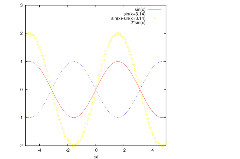
Figure 2: The 3 phase supply carrying voltage of peak value, ${\rm V_{m}}$ can be used to generate voltage of peak value ${\rm 2V_{m}}$.

$$V_{AB} = V_{m}sin(\theta)-V_{m}sin(\theta+\phi)$$

$$= -2V_{m}cos\left({2\theta+\phi\over 2}\right)sin\left({\phi\over 2}\right)$$

where ${\rm V_{m}}$ is the peak voltage and ${\rm\phi}$ the phase difference between the two phases. For a 2-phase supply, where the phase difference between the two waveforms is ${\rm\pi}$, the potential difference would be

$$V_{AB} = -2V_{m}cos\left(\theta+{\pi\over 2}\right)sin\left({\pi\over 2}\right)$$

$$= 2V_{m}sin(\theta)$$

This mathematics is graphically represented in fig 2. It can be appreciated that the power delivered to the load now would be ${\rm 2V_{m}^{2}/R_{L}}$. This example shows how polyphase transmissions delivers more power.

While these are important issues to be appreciated by a physicist setting up a laboratory with instruments that require high power, schools and colleges do not help develop this concept with hand-on experimentation for fear of possible accidents that could even prove fatal. While kits are present in engineering colleges for electrical engineering, not much is found in the literature in way of simple experiemnts for physics and electronics students. In this direction, we have designed and tested a simple circuit, where two phases are generated from a sinusodial wave taken from a function generator.

Figure 3: Simple circuit for simulating the 3-phase supply used in modern power distribution.

The Circuit

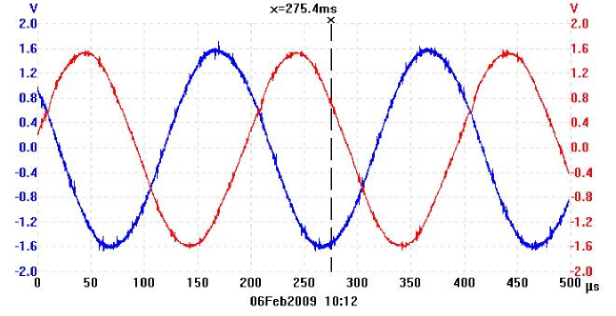
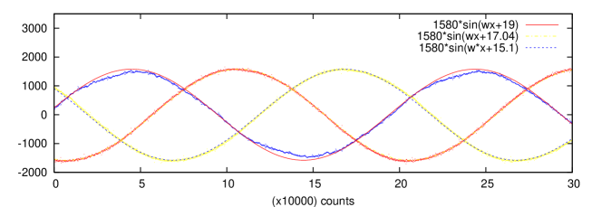
Figure 4: The two Phases (A and C) as seen by the dual trace picoscope 2202. Also, shown is the generated 3-phase supply using sinusodial wave from function generator (Phase A) and Phase B and Phase C using phase shift circuits.

The proposed circuit requires three opamps, of which the first opamp is assembled in an inverting configuration [2]. The sinusodial input from a function generator (shown in fig 3 as ‘1’) is given as an input to this inverting amplifier. This signal also acts as one of the 3 phases, namely phase A. The gain of this amplifier is kept as unity with ${\rm R_{1}=100K\Omega}$. This circuit acts as a buffer preventing any loading by successive circuits and introduces a phase change of ${\rm\pi}$ between output and input waveforms (as indicative of the name “inverting” amplifier).

The RC circuit is designed to introduce a phase difference of ${\rm 120^{o}}$ for the selected frequency. However, a single combination of RC can at the most introduce a phase difference equal to or less than ${\rm 90^{o}}$. Hence, two sections are used, with each RC section introducing a phase shift of ${\rm 60^{o}}$. The values of R and C are selected using the formula [3]

$$RC={1\over\omega tan\phi}$$ (2)

In our study, for an 5KHz wave provided from the function generator, we selected ${\rm R=18K\Omega}$ and ${\rm C=0.001\mu F}$. Hence points ‘3’ and ‘4’ of the circuit would be ${\rm 240^{o}\,(=180^{o}+60^{o})}$ and ${\rm 300^{o}\,(=240^{o}+60^{o})}$ respectively out of phase with respect to the input. The impedence networks act as potential dividers and hence the voltage levels at ‘3’ and ‘4’ would be lower than that given as input. Since the three phases would have the same amplitude, the signals at ‘3’ and ‘4’ would have to be amplified. We use as inverting amplifier again for point ‘4’. The voltage gain of this amplifier is give by ${\rm R_{f}/R_{1}}$. Hence, ${\rm R_{f}}$ has to be varied till the voltage signals amplitude is identical to the input signal. Also, this inverting amplifier introduces a phase change of ${\rm\pi}$. The net phase difference hence would be ${\rm 480^{o}\,(=300^{o}+180^{o})}$ which is nothing but a phase difference of ${\rm 120^{o}\,(=2\pi^{o}+120^{o})}$. The output of this op amp circuit would be phase ‘B’.

Similar amplitude correction is required for the wave collected at point ‘3’. However, here we select a non-inverting amplifier circuit whose gain is given as ${\rm 1+R_{fo}/R_{1}}$ and as the name suggests does not introduce any further phase shifts (${\rm R_{f}}$ and ${\rm R_{fo}}$ used were ${\rm 1M\Omega}$ pots and typically had values greater than ${\rm 100K\Omega}$). Hence, the net shift at the output remains the same as that at point ‘3’ at ${\rm 240^{o}}$ or ${\rm 240^{o}\,(=2\pi-120^{o})}$. This is phase C of the simulated 3-phase supply.

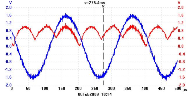
Figure 5: A half-wave rectification circuit for three phase supply. The output waveform of this circuit shows that the ripples would be less than the case of half-wave rectification of a single phase supply.

Fig 4 shows the waveforms (phase A and C) as captured by Picoscope (Model 2202). Since the model only gives dual trace, only two waves can be shown simultaneously. However, the data captured by Picoscope shows all three phases simultaneously. Curve fitting these data points give the phase difference between the various phases to be 1.95radians or ${\rm\sim 112^{o}}$. Also, the peak voltage (${\rm V_{m}}$) also works out to be 1.58v.

While the circuits achieves the purpose of mimicing a 3-phase supply, experiments can be done to further understand applications of 3-phase supply. For example, one can study the rectification and advantage of generating DC from 3-phase supply. For this, all one needs is 3 diodes and a load resistance (see fig 5). The output waveform is DC and also notice even without any filtering circuit, the output is continuous with little ripple. This is because, as seen by the load, the input frequency is three times that of a single phase supply. The ripples in a rectified output is inversely proportional to the frequency [3], hence the low ripples here can be understood. Also, this output gives visual idea and helps in easier understanding that each phase in a 3-phase supply is separated by ${\rm 120^{o}}$. In this rectifier circuit, only that diode conducts, for which the phase connected to it has the highest instantaneous potential with respect to the neutral. Fig 4 shows one phase to have highest potential with repect to the other phases for ${\rm 120^{o}}$. Thus, in one cycle (${\rm 2\pi}$) there would be three peaks of the output DC wave. This is visiable in fig 5.

Conclusion

A simple circuit has been proposed to demonstrate the behaviour of 3-phase power distribution. The simple circuit discussed in this article cost Rs (Indian Rupee) 20/- to assemble (less than a dollar) and can be a very usual experiment in schools and under-graduate laboratorys to learn more about 3-phase supply and it’s application.

References

- [1] Anil K. Rajvanshi, Resonance (India) 12 (2007) p4.
- [2] Ramakant A. Gayakwad, “Operational Amplifiers and linear integrated circuits”, Edition, Prentice Hall India (Indiam 2002).
- [3] P.Arun, “Electronics”, Narosa (New Delhi) 2005.