New procedures for testing whether stock price processes are martingales

Abstract

We propose procedures for testing whether stock price processes are martingales based on limit order type betting strategies. We first show that the null hypothesis of martingale property of a stock price process can be tested based on the capital process of a betting strategy. In particular with high frequency Markov type strategies we find that martingale null hypotheses are rejected for many stock price processes.

Keywords and phrases: betting strategy, efficient market hypothesis (EMH), game-theoretic probability, sequential test.

1 Introduction

The efficient market hypothesis (EMH), that no one with finite capital can consistently outperform the market, is the fundamental assumption in the theory of financial engineering. In mathematical finance the efficient market hypothesis is formulated as the martingale property of price processes of tradable assets such as stocks.

Often the martingale assumption is replaced by a more convenient assumption of “random walk”. Although exact formulation of random walk depends on literature (e.g. [2, Chapter 2], [1]), the usual assumption is that the price process observed at equi-spaced time points has independent increments with mean zero, after adjustment of the systematic trend. However there are many empirical studies showing that stock price processes are not random walks (e.g. [2], [9]).

Note that the class of martingales is larger than the class of random walks with zero expected increment ([8]). This implies that rejecting the hypothesis of random walk does not necessarily mean rejecting the hypothesis of martingale. Therefore it is desirable to directly test the martingale assumption of stock price processes without assuming a random walk.

We propose to test the martingale hypothesis of price processes based on our previous works on “limit order” type betting strategies ([16, 17]) in the framework of game-theoretic probability by Shafer and Vovk ([14]) and an adaptation of the result by Dubins and Schwarz [4] to positive measure-theoretic martingales. As discussed in Section 2.1, betting strategies in game-theoretic probability naturally yield sequential testing procedures for the measure-theoretic martingale hypothesis. Moreover our strategies in [16, 17] are of very simple form and provide convenient testing procedures.

Our testing procedures depend on the direction of a price process (“ups” and “downs”) at times, when the process hits fixed horizontal grids of prices. We call these time points hitting times. Thus our procedures are very much different from procedures based on increments of price processes observed at equi-spaced time points.

One advantage of our testing procedure (compared to equi-spaced procedures) is that we do not have to worry about specifications of distributions of the increments, such as the the heaviness of the tail of the distribution of the increments, because in our procedures the amount of the increments are fixed by the given grids of prices. Our procedure depends only on the ups or the downs of the price process between hitting times. This is contrasted with problems of model specifications for testing EMH in standard approaches (e.g. [18]).

Our approach is similar to the approach of testing EMH based on algorithmic complexity of the ups and downs of price processes in [15] and [5]. In fact, it is well known that betting strategies and compression algorithms of binary strings are essentially equivalent [3, Chapter 6]. However the approaches of [15] and [5] are based on price movements observed at equi-spaced time points and therefore they are different from ours.

The organization of this paper is as follows. In Section 2 we summarize results on betting strategies in the framework of game-theoretic probability of Shafer and Vovk ([14]) and explain that these betting strategies naturally lead to sequential testing procedures for the null hypothesis of measure-theoretic martingale. In Section 3 we propose our procedure for testing martingale properties of price processes based on limit order type betting strategies. We give numerical results of testing martingale properties of some Japanese stock price processes in Section 4, where numerical examinations are also added for the effect of transaction costs on capital processes. We conclude our paper with some remarks in Section 5.

2 Preliminary results

In this section we give an exposition on betting strategies in game-theoretic probability based on our earlier results in [7], [16] and [17]. In Section 2.1 we also remark the important fact that these betting strategies can be used for testing the null hypothesis of measure-theoretic martingale.

2.1 Prudent strategies in game-theoretic probability and a sequential test of measure-theoretic martingale hypothesis

For simplicity of exposition we consider the biased-coin tossing game. This game is a discrete time game played by two players called “Investor” and “Market”. Investor enters the game with the initial capital of ${\cal K}_{0}=1$. For each round Investor first decides how much to bet and then Market (after seeing the Investor’s move) decides the outcome. In the biased-coin tossing game, the outcome chosen by Market is either 1 (“up”) or 0 (“down”). The formal protocol of the game is written as follows.

Biased-Coin Game
Protocol:

${\cal K}_{0}=1$ and $0<\rho<1$ are given.
FOR $n=1,2,\dots$:
Investor announces $\nu_{n}\in{\mathbb{R}}$.
Market announces $x_{n}\in\{0,1\}$.
${\cal K}_{n}={\cal K}_{n-1}+\nu_{n}(x_{n}-\rho)$.
END FOR

We call $\rho$ the risk-neutral probability. Investor can choose $\nu_{n}$ based on the past moves $x_{1},\dots,x_{n-1}$ of Market. Suppose that Investor adopts a strategy ${\cal P}$, which is a function specifying $\nu_{n}$ based on $x_{1},\dots,x_{n-1}$ with some initial value $\nu_{1}$.

$${\cal P}:(x_{1},\dots,x_{n-1})\mapsto\nu_{n}.$$

Then Investor’s capital at the end of round $n$ is written as

$${\cal K}_{n}^{{\cal P}}={\cal K}_{0}+\sum_{i=1}^{n}{\cal P}(x_{1},\dots,x_{i-1})(x_{i}-\rho).$$ (1)

A betting strategy ${\cal P}$ of Investor is called prudent if Investor is never bankrupt when using ${\cal P}$, i.e. ${\cal K}_{n}^{{\cal P}}\geq 0$ for all $n$ and for all $x_{1},x_{2},\dots\in\{0,1\}$.

In the framework of game-theoretic probability of Shafer and Vovk ([14]) there is no probabilistic assumption on the behavior of Market. Therefore Market in the above biased-coin game may even be adversarial to Investor. However the usual measure-theoretic assumption on the behavior of Market is that Market is oblivious to Investor’s moves and chooses $x_{n}$ independently as $P(x_{n}=1)=\rho=1-P(x_{n}=0)$, ignoring Investor’s bet $\nu_{n}$. We write this null hypothesis as

$$H:p_{1}=\rho,$$ (2)

where $p_{1}=P(x_{n}=1)$. Note that the mutual independence of $x_{n}$, $n=1,2,\dots$, is also implied by $H$ for the biased-coin game, because the outcome $x_{n}$ is binary. If ${\cal P}$ is a prudent strategy, then under $H$, ${\cal K}^{{\cal P}}_{n}$ is a usual measure-theoretic non-negative martingale.

By the Markov inequality for non-negative measure-theoretic martingales (cf. Chapter II, Section 57 of [13]) we have the following sequential testing procedure for $H$.

Proposition 2.1.

Let $0<\alpha<1$ be given. Reject the null hypothesis $H:p_{1}=\rho$ as soon as ${\cal K}^{{\cal P}}_{n}\geq 1/\alpha$, where ${\cal P}$ is a prudent strategy. This procedure has the significance level $\alpha$.

The intuitive interpretation of this proposition is as follows. $H$ corresponds to the efficient market hypothesis (EMH). Investor can disprove EMH by beating Market, i.e., if he can multiply his capital many times by an appropriate betting strategy. If Investor can make his capital 100 times larger than his initial capital ${\cal K}_{0}$, then $H$ is rejected at the significance level of 1%.

We can also use Ville’s inequality (Section 2.5 of [14], page 100 of [19]), which is now commonly known as Doob’s supermartingale inequality ((57.10) of [13]). From game-theoretic viewpoint the following procedure is not very much different from the procedure in the above proposition, because it corresponds to stop betting after the hitting time ${\cal K}^{{\cal P}}_{n}\geq 1/\alpha$.

Proposition 2.2.

Let $0<\alpha<1$ be and $N>0$ be given. Reject the null hypothesis $H:p_{1}=\rho$ if $\max_{0\leq n\leq N}{\cal K}^{{\cal P}}_{n}\geq 1/\alpha$, where ${\cal P}$ is a prudent strategy. This procedure has the significance level $\alpha$.

We have stated the above propositions for the protocol of biased-coin game. However as in [14] we can consider more complicated protocols, such as the bounded-forecasting game, where for each round Market chooses $x_{n}$ in the bounded interval $[0,1]$. The measure-theoretic interpretation of the null hypothesis $H$ in (2) is that $x_{n}-\rho$, $n=1,2,\dots$, are (uniformly bounded) martingale differences. In this form, the null hypothesis $H$ does not place any distributional assumptions on $x_{n}$, except for the martingale property. Therefore we are directly testing the assumption of martingale property. As long as ${\cal P}$ is a prudent strategy, we can test $H$ by Proposition 2.1.

2.2 Limit order type strategy in continuous time game and embedded coin-tossing game

Although the biased-coin game of the previous subsection is very simple, we can analyze a continuous time game between Investor and Market with the biased-coin game of the previous subsection, by embedding it into continuous time by a limit order type strategy.

Consider a continuous time game between Investor and Market. Market chooses a price path $S(t)$, $t\geq 0$, of a financial asset. We assume that $S(t)$ is continuous and positive. Investor enters the market at time $t=t_{0}=0$ with the initial capital of ${\cal K}(0)=1$ and he will buy or sell any amount of the asset at discrete time points $0=t_{0}<t_{1}<t_{2}<\cdots$. Let $M_{i}\in{\mathbb{R}}$ denote the amount of the asset he holds for the time interval $[t_{i},t_{i+1})$. Then the capital of Investor ${\cal K}(t)$ at time $t$ is written as

$${\cal K}(0)=1,$$

$${\cal K}(t)={\cal K}(t_{i})+M_{i}(S(t)-S(t_{i}))\quad\textrm{for}\ \ t_{i}\leq t<t_{i+1}.$$ (3)

By defining $\theta_{i}=M_{i}S(t_{i})/{\cal K}(t_{i})$, we rewrite (2.2) as

$${\cal K}(t)={\cal K}(t_{i})\left(1+\theta_{i}\frac{S(t)-S(t_{i})}{S(t_{i})}\right)\quad\textrm{for}\ \ t_{i}\leq t<t_{i+1}.$$

In limit order type strategy, Investor takes some constant $\delta>0$ and decides the trading times $t_{1},t_{2},\dots$ as follows. After $t_{i}$ is determined, let $t_{i+1}$ be the first time after $t_{i}$ when either

$$\frac{S(t_{i+1})}{S(t_{i})}=1+\delta\quad\textrm{or}\quad=\frac{1}{1+\delta}$$

happens. Let $w_{i}=t_{i+1}-t_{i}$ denote the waiting times between two successive trading times. In terms of $\log S$, the waiting times $w_{i}$ are determined by

$$\log S(t_{i+1})-\log S(t_{i})=\pm\eta,\quad\eta=\log(1+\delta)\qquad(\delta=e^{\eta}-1).$$ (4)

This process leads to a discrete time coin-tossing game embedded in the continuous time game in the following manner. Let

$$x_{n} =\frac{(1+\delta)S(t_{n+1})-S(t_{n})}{\delta(2+\delta)S(t_{n})}=\begin{cases}1,&\text{if}\ S(t_{n+1})=S(t_{n})(1+\delta),\\ 0,&\text{if}\ S(t_{n+1})=S(t_{n})/(1+\delta),\end{cases}$$ (5)

and

$$\rho=\frac{1}{2+\delta},\quad\tilde{{\cal K}}_{n}={\cal K}(t_{n+1}),\quad\nu_{n}=\frac{\delta(2+\delta)}{1+\delta}\theta_{n}.$$

Now we have the following discrete time coin-tossing game.

Embedded Discrete Time Coin-Tossing Game
Protocol:

$\tilde{{\cal K}}_{0}:=1$.
FOR $n=1,2,\dots$:
Investor announces $\nu_{n}\in{\mathbb{R}}$.
Market announces $x_{n}\in\{0,1\}$.
$\tilde{{\cal K}}_{n}=\tilde{{\cal K}}_{n-1}(1+\nu_{n}(x_{n}-\rho))$.
END FOR

Combining the embedded discrete time coin-tossing game with Proposition 2.1, we can test whether a continuous price process chosen by Market is a measure-theoretic martingale. Suppose that the price process $S(t)$ of Market is a positive measure-theoretic martingale. We write this null hypothesis as

$$\bar{H}:S(t)\text{\ is a positive martingale.}$$ (6)

Under $\bar{H}$, for every $\delta>0$, $x_{n}$’s in the embedded coin-tossing game satisfy the null hypothesis $H$ in (2) with $\rho=1/(2+\delta)$. Therefore any prudent strategy for the embedded coin-tossing game can be used as a sequential testing procedure of $\bar{H}$ by Proposition 2.1. A particularly useful betting strategy can be given from Bayesian viewpoint as shown in the next section.

2.3 Bayesian betting strategy based on past number of ups and downs

A simple betting strategy for the biased-coin game is given by a Bayesian consideration ([7]). By the embedded coin-tossing game, it can be applied to the continuous time game.

Let $h_{n}=n\bar{x}_{n}=\sum_{i=1}^{n}x_{i}$ denote the number of heads and let $t_{n}=n-h_{n}$ denote the number of tails up to round $n$ in the biased-coin game. Fix $a>0,b>0$. We call the following strategy of Investor a beta-binomial strategy (with the hyperparameters $a,b$):

$$\nu_{n}=\frac{\hat{p}_{n}^{Q}-\rho}{\rho(1-\rho)}\qquad\text{where}\quad\hat{p}_{n}^{Q}=\frac{a+h_{n-1}}{a+b+n-1}.$$ (7)

The capital process ${\cal K}_{n}$ for this strategy is explicitly written as

$${\cal K}_{n}=\frac{(a)_{h_{n}}(b)_{t_{n}}}{(a+b)_{n}\rho^{h_{n}}(1-\rho)^{t_{n}}},$$ (8)

where

$$(c)_{l}=c(c+1)\cdots(c+l-1)=\frac{\Gamma(c+l)}{\Gamma(c)}$$

for $c>0$ and non-negative integer $l$. Since ${\cal K}_{n}$ in (8) is always non-negative, we have a sequential test of $H$ by Proposition 2.1.

An advantage of the beta-binomial strategy is that the asymptotic behavior of the capital process is easy to study by Stirling’s formula. When $n,h_{n}$ and $t_{n}$ are all large, we can evaluate the log capital as

$$\log{\cal K}_{n}=nD\left(\frac{h_{n}}{n}\Big{\|}\rho\right)-\frac{1}{2}\log n+O(1),$$

where

$$D(p\|q)=p\log\frac{p}{q}+(1-p)\log\frac{1-p}{1-q}$$

denotes the Kullback-Leibler information between $0<p<1$ and $0<q<1$.

Now we move onto the embedded coin-tossing game. Suppose that Investor trades in a finite time interval $[0,T]$ and he uses the Bayesian strategy in (7) for the embedded coin-tossing game. We define $n^{*}=n^{*}(T,\delta,S(\cdot))$ by $t_{n^{*}}<T\leq t_{n^{*}+1}$. Investor’s capital ${\cal K}(T)={\cal K}^{{\cal P}^{\delta,a,b}}(T,S(\cdot))$ at $t=T$ for large $n^{*}$ is written as

$${\cal K}(T)=\tilde{{\cal K}}^{*}_{n^{*}}\left(1+\theta_{n^{*}}^{*}\frac{S(T)-S(t_{n^{*}})}{S(t_{n^{*}})}\right),\quad\theta_{n^{*}}^{*}=\frac{1+\delta}{\delta(2+\delta)}\nu_{n^{*}}^{*}.$$

Since $\left|\frac{S(T)-S(t_{n^{*}})}{S(t_{n^{*}})}\right|<\delta$, we have

$$\log{\cal K}(T)=\log\tilde{{\cal K}}^{*}_{n^{*}}+O(1)=n^{*}D\left(\frac{h_{n^{*}}}{n^{*}}\Big{\|}\rho\right)-\frac{1}{2}\log n^{*}+O(1).$$ (9)

2.4 Generality of high-frequency limit order strategy

This subsection is a part which is rather independent of the previous sections. Here we show a generality of the high-frequency limit order strategy developed in [16], which implies that when the asset price $S(t)$ follows the geometrical Brownian motion, our strategy automatically incorporates the well-known constant proportional betting strategy originated with Kelly ([6]) and yields the likelihood ratio in the Girsanov’s theorem for geometric Brownian motion. The convergence results in this subsection are of measure-theoretic almost everywhere convergence.

Let $S(t)$ be subject to the geometrical Brownian motion with drift $\mu$ and volatility $\sigma$. Then

$$\log S(T)-\log S(0)=\bigg{(}\mu-\frac{1}{2}\sigma^{2}\bigg{)}T+\sigma W(T),$$

where $W(\cdot)$ denotes the standard Brownian motion. In the following we write

$$L(T)=\log S(T)-\log S(0).$$

We let $T\rightarrow\infty$ and let $\eta=\eta_{T}$ depend on $T$ in such a way that $|\log\eta_{T}|=o(\sqrt{T})$. Similarly we denote $\delta_{T}=e^{\eta_{T}}-1$, $\rho_{T}=1/(2+\delta_{T})$. Define

$$TV(\eta_{T},T)=\sum_{i=1}^{n^{*}}|\log S(t_{i})-\log S(t_{i-1})|,\quad L(\eta_{T},T)=\log S(t_{n^{*}})-\log S(0),$$

$$\qquad\qquad\zeta(\eta_{T},T)=\frac{L(\eta_{T},T)}{TV(\eta_{T},T)}.$$

We call $TV(\eta_{T},T)$ the total $\eta$-variation of $\log S(t)$ in the interval $[0,T]$. Then we have

$$\eta_{T}TV(\eta_{T},T)=n^{*}\eta_{T}^{2}=\sigma^{2}T+O(\eta_{T}),$$

and hence we can evaluate

$$\theta_{n^{*}}^{*}=\frac{\mu}{\sigma^{2}}+\frac{W(T)}{\sigma T}+O(\eta_{T}).$$

Note that when $L(T)$ is a process symmetric around the origin with $\mu-\frac{1}{2}\sigma^{2}=0$, we have

$$\theta_{n^{*}}^{*}=\frac{1}{2}+\frac{W(T)}{\sigma T}+O(\eta_{T}),$$

and the main term $1/2$ in the right-hand side indicates the even rebalanced strategy between the asset and the cash.

Let us consider $n^{*}D(p(\eta_{T},T)\|\rho_{T})$, where $n^{*}=TV(\eta_{t},T)/\eta_{T}$, $p(\eta_{T},T)=h_{n^{*}}/n^{*}=(1+\zeta(\eta_{T},T))/2$. From the Taylor expansion

$$D\left(\frac{1+d_{1}}{2}\Big{\|}\frac{1+d_{2}}{2}\right)=\frac{1}{2}(d_{1}-d_{2})^{2}+O(|d_{1}-d_{2}|^{3}),$$

with $d_{1}=\zeta(\eta_{T},T),\ d_{2}=-\delta_{T}/2$, we have

$$n^{*}D\left(p(\eta_{T},T)\|\rho_{T}\right) =\frac{n^{*}}{2}\bigg{(}\zeta(\eta_{T},T)+\frac{\delta_{T}}{2}\bigg{)}^{2}+O(\eta_{T}^{3})=\frac{n^{*}\eta_{T}^{2}}{2}(\theta_{n^{*}}^{*})^{2}+O(\eta_{T}^{3})$$

$$=\frac{\sigma^{2}T}{2}\bigg{(}\frac{\mu}{\sigma^{2}}+\frac{W(T)}{\sigma T}\bigg{)}^{2}=\frac{\mu W(T)}{\sigma}+\frac{\mu^{2}T}{2\sigma^{2}}+\frac{W^{2}(T)}{2T}+O(\eta_{T}^{3}).$$

The log capital $\log{\cal K}(T)=n^{*}D\left(p(\eta_{T},T)\|\rho_{T}\right)-\frac{1}{2}\log n^{*}+O(1)$ is expressed as

$$\log{\cal K}(T)=\frac{\mu W(T)}{\sigma}+\frac{\mu^{2}T}{2\sigma^{2}}-\frac{1}{2}\log T+\log\eta_{T}+O(1),$$

and hence when $|\log\eta_{T}|=o(\sqrt{T})$, the main terms in the right-hand side of $-\log{\cal K}(T)$,

$$-\log{\cal K}(T)=-\frac{\mu W(T)}{\sigma}-\frac{\mu^{2}T}{2\sigma^{2}}+o(\sqrt{T})$$

provide the likelihood ratio of the unique martingale measure known as the Girsanov’s theorem, and we obtain

$$\lim_{T\to\infty}\frac{\log{\cal K}(T)}{T}=\frac{\mu^{2}}{2\sigma^{2}}.$$

2.5 Markov betting strategy

The Bayesian strategy in previous subsections is a simple strategy based on the past number of ups and downs only. The strategy does not exploit possible autocorrelations in the ups and downs of the price process. Multistep Bayesian strategy, in particular the Markov type strategy in [17] is very efficient in exploiting possible autocorrelations. In this paper we just use the first-order Markov strategy.

For the biased-coin game the strategy is given as

$$\nu_{1}=0,\quad\nu_{n}=\begin{cases}\nu_{n}^{+},&\textrm{if}\ x_{n-1}=1\\ \nu_{n}^{-},&\textrm{if}\ x_{n-1}=0\end{cases}\quad n=2,3,\dots,$$

where $\nu_{n}^{+}$ and $\nu_{n}^{-}$ can have different values. It incorporates the information on the last move $x_{n-1}$ of Market.

We use the beta-binomial strategy separately for the case of $x_{n-1}=1$ and $x_{n-1}=0$ with hyperparameters $a,b$. Let $q_{n}^{1}=h_{n}$ and $q_{n}^{0}=n-h_{n}$. Denote the numbers of pairs $(x_{i-1}x_{i})=(11),(10),(01),(00)$, $i=2,\dots,n$, by $q_{n}^{11},\ q_{n}^{10},\ q_{n}^{01},\ q_{n}^{00}$, respectively. The capital ${\cal K}_{n}={\cal K}_{n}^{{\cal P}_{Q}}$ for this strategy is given by

$${\cal K}_{n} =\frac{\Gamma(a+b)^{2}\Gamma(q_{n}^{11}+a)\Gamma(q_{n}^{10}+b)\Gamma(q_{n}^{01}+a)\Gamma(q_{n}^{00}+b)}{\Gamma(a)^{2}\Gamma(b)^{2}\Gamma(q_{n}^{11}+q_{n}^{10}+a+b)\Gamma(q_{n}^{01}+q_{n}^{00}+a+b)\rho^{q_{n}^{11}+q_{n}^{01}}(1-\rho)^{q_{n}^{10}+q_{n}^{00}}}.$$

By Stirling’s formula the asymptotic behavior of ${\cal K}_{n}$ is easily derived.

We can apply the above first-order Markov strategy to the embedded coin-tossing game for continuous price paths. In [17] the performance of the strategy for small grid size $\delta$ is analyzed as follows. Under some regularity conditions, if the price process path has the Hölder exponent $H\neq 1/2$, then

$$\log{\cal K}_{n^{*}}=n^{*}D\Big{(}\frac{1}{2^{1/H-1}}\Big{\|}\frac{1}{2}\Big{)}+o(n^{*}).$$ (10)

3 Tests of martingale property

In Section 2.2 we have already shown that we can test $\bar{H}$ in (6) by limit order type betting strategy. It is an important fact that the converse is also true. If the null hypothesis $H$ in (2) holds for embedded discrete time coin-tossing game for every $\delta>0$, then $\bar{H}$ holds. This fact can be proved by adapting the result of Dubins and Schwartz [4] to positive martingales. A more rigorous and modern treatment of the result of Dubins and Schwartz is given in Chapter V of [11]. Recently Vovk [20] gave a complete generalization of these results to game-theoretic framework. However for our purposes, the arguments given in [4] are sufficient and more suitable, because they are based on similar ideas to our limit order type strategies.

Proposition 3.1.

Let $S(t)$, $t\geq 0$, be a continuous positive stochastic process with $S(0)=1$ such that almost all of whose paths are nowhere constant and $\limsup_{t}S(t)=\infty$, $\liminf_{t}S(t)=0$. Then the following three conditions are equivalent.

1. $S$ is a martingale.

2. $S$ is a path-dependent and future-independent time change of the standard geometric Brownian motion.

3. For every $\eta>0$, the directions $x_{j}$, $j=1,2,\dots$, in (5) are independently and identically distributed with

   $$P(x_{j}=1)=\frac{1}{1+e^{\eta}}$$

   and they are independent of the waiting times $\{w_{j},j=1,2,\dots\}$.

Proof.

Since our proof is a simple adaptation of the proof in [4] we only give an outline of the proof. The implications 2 $\Rightarrow$ 1 and 1 $\Rightarrow$ 3 are obvious. Therefore it suffices to prove 3 $\Rightarrow$ 2. By examining the proof in [4], we note that the only difference in our proof is the finite dimensional distributions of $\log S(t)$ at the trading times $t_{1},t_{2},\dots$. For simplicity we consider the distribution of $\log S(t_{2})-\log S(t_{1})$ for any fixed $\eta$. Now consider a sequence of increasingly finer horizontal grids $\eta_{m}=2^{-m}\eta$ in the logarithmic scale for $\log S$. Then $\log S(t_{2})-\log S(t_{1})$ ca be written

$$\log S(t_{2})-\log S(t_{1})=\sum_{j=1}^{2^{m}}\epsilon_{mj}\eta_{m},$$

where $\epsilon_{mj}$, $j=1,\dots,2^{m}$, are i.i.d. $\pm 1$ random variables with $P(\epsilon_{ml}=1)=1/(1+e^{\eta_{m}})$. The mean and the variance of $\sum_{j=1}^{2^{m}}\epsilon_{mj}\eta_{m}$ are given by

$$2^{m}(2p_{mj}-1),\quad 4\times 2^{m}p_{mj}(1-p_{mj}),\qquad\big{(}\ p_{mj}=\frac{1}{1+e^{\eta_{m}}}\ \big{)}.$$

As $m\rightarrow\infty$, these converge to $-\eta/2$ and $\eta$, respectively. Also by the central limit theorem $\log S(t_{2})-\log S(t_{1})$ is distributed according to $N(-\eta/2,\eta)$. Considering any finite number trading times, we see that finite-dimensional distributions are the same as the geometric Brownian motion. Now an argument similar to [4] shows that $S$ satisfies 2. ∎

Because of Proposition 3.1 it is natural to test the martingale hypothesis (6) by testing that the directions $x_{j}$, $j=1,2,\dots$, are i.i.d. {0, 1} valued random variables with the probability $P(x_{j}=1)=1/(1+e^{\eta})$. Note that we can interpret the distribution of the waiting times as nuisance parameters of the null hypothesis.

In the next section we use two strategies and associated sequential tests. The first strategy is a simple Bayesian strategy of Section 2.3 concerning the success probability $P(x_{j}=1)=1/(1+e^{\eta})$. The second strategy is the first-order Markov strategy of Section 2.5 for testing independence.

4 Numerical examples

In this section we give some numerical examples on the stock price data from the Tokyo Stock Exchange. The data are the stock minute prices from June 1st to July 31st in 2006 for three Japanese companies SoftBank, IHI, and Sony listed on the first section of the TSE, which were adapted from Bloomberg LP. Usually there are 270 minute price data a day.

We employed a simple Bayesian strategy and a Markov strategy. The former did not show significant results. This is because the empirical probabilities of heads ($p^{1}({\rm ft})$ in Table 1) are close to $0.5$. However we obtained significant results by the first-order Markov strategy for three companies with common values $\eta=2^{-k},\ a,b=0.01\cdot 2^{k},\ k=8$. The results are shown in Figures 1–15. Figures 1–5 are for SoftBank, Figures 6–10 are for IHI and Figures 11–15 are for Sony. In each figure, fn denotes the first round such that the Markov capital MK satisfies $\textrm{MK(fn)}\geq 10^{3}$, and ft denotes the approximate time of fn in minutes. By Proposition 2.1, $10^{3}$ corresponds to the significance level of $\alpha=0.1\%$.

We also exhibit processes of empirical probabilities $p^{1|1},p^{0|0},p^{1}$, and processes of Hölder exponents $H^{1},H^{0}$, which are given in the following manner.

$$p^{1|1}_{n}=\frac{q^{11}_{n}}{q^{1}_{n}},\quad p^{0|0}_{n}=\frac{q^{00}_{n}}{q^{0}_{n}},\quad p^{1}_{n}=\frac{q^{1}_{n}}{n},$$

$$\frac{1}{2^{1/H^{1}_{n}}-1}=p^{1|1}_{n},\quad\frac{1}{2^{1/H^{0}_{n}}-1}=p^{0|0}_{n}.$$ (11)

The relation (4) between the conditional probability and the Hölder exponent is one of the results obtained in [17]. These typical values are summarized in Table 1.

Figure 1 : Minute prices of SoftBank

Figure 2 : Capital process of Markov

strategy

Figure 3 : Log capital process of Markov

strategy

Figure 4 : Processes of empirical

probabilities $p^{1|1},\ p^{0|0},\ p^{1}$

Figure 5 : Processes of Hölder exponents

$H^{1},H^{0}$

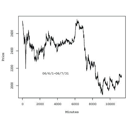
Figure 1: SoftBank minute prices

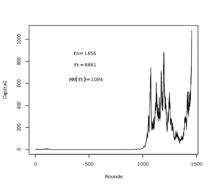
Figure 2: Markov capital process

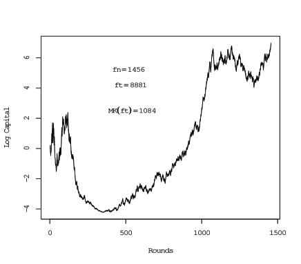
Figure 3: Log Markov capital process

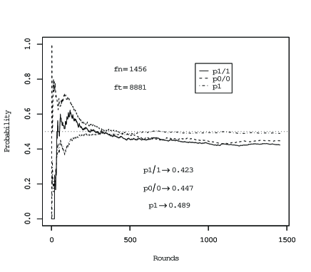
Figure 4: Empirical probability processes

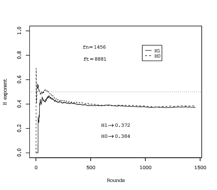
Figure 5: Hölder exponent processes

Figure 6 : Minute prices of IHI

Figure 7 : Capital process of Markov

strategy

Figure 8 : Log capital process of Markov

strategy

Figure 9 : Processes of empirical

probabilities $p^{1|1},\ p^{0|0},\ p^{1}$

Figure 10 : Processes of Hölder exponents

$H^{1},H^{0}$

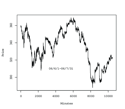
Figure 6: IHI minute prices

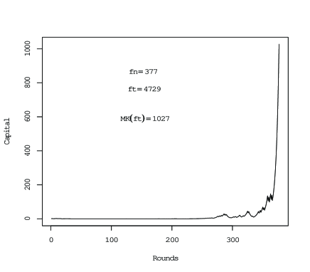
Figure 7: Markov capital process

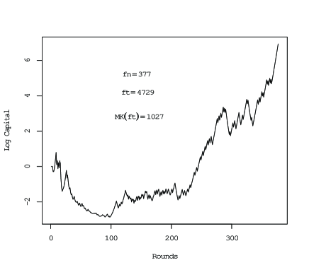
Figure 8: Log Markov capital process

Figure 9: Empirical probability processes

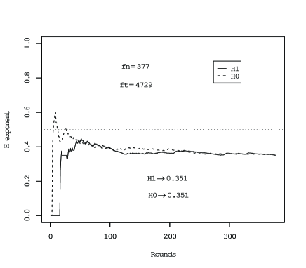
Figure 10: Hölder exponent processes

Figure 11 : Minute prices of Sony

Figure 12 : Capital process of Markov

strategy

Figure 13 : Log capital process of Markov

strategy

Figure 14 : Processes of empirical

probabilities $p^{1|1},\ p^{0|0},\ p^{1}$

Figure 15 : Processes of Hölder exponents

$H^{1},H^{0}$

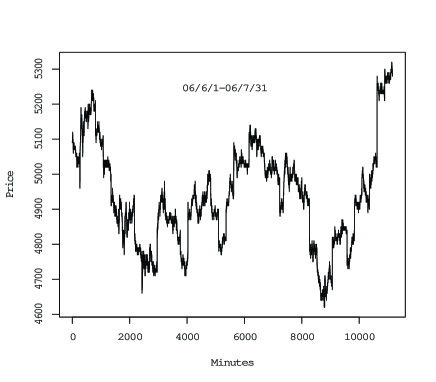
Figure 11: Sony minute prices

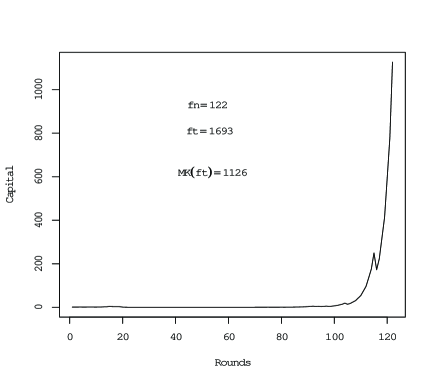
Figure 12: Markov capital process

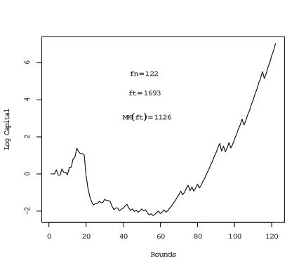
Figure 13: Log Markov capital process

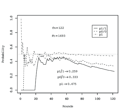
Figure 14: Empirical probability processes

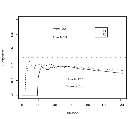
Figure 15: Hölder exponent processes

Table 1: Typical values for three stock minute prices

	fn	ft	MK(ft)	$p^{1|1}$(ft)	$p^{0|0}$(ft)	$p^{1}$(ft)	$H^{1}$(ft)	$H^{0}$(ft)
SoftBank	1456	8881	1084	0.423	0.449	0.489	0.372	0.384
IHI	377	4729	1027	0.378	0.378	0.499	0.351	0.351
Sony	122	1693	1126	0.259	0.333	0.475	0.295	0.330

Figure 16 : Log capital processes of Markov

strategy with costs : SoftBank

Figure 17 : Log capital processes of Markov

strategy with costs : IHI

Figure 18 : Log capital processes of Markov

strategy with costs : Sony

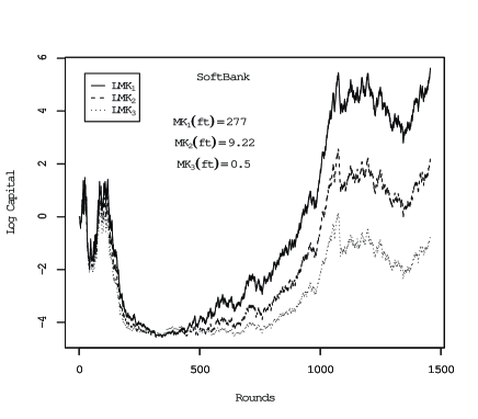
Figure 16: Log Markov capitals with costs

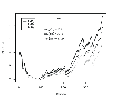
Figure 17: Log Markov capitals with costs

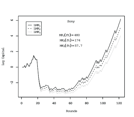
Figure 18: Log Markov capitals with costs

Table 2: Capital values for three stock minute prices with costs $(\eta=2^{-8})$

	fn	$\textrm{MK}_{1}$(ft)	hn	$\textrm{MK}_{2}$(ft)	hn	$\textrm{MK}_{3}$(ft)	hn
SoftBank	1456	277	326	9.22	551	0.50	636
IHI	377	209	25	39.3	103	5.09	129
Sony	122	480	10	174	20	57.7	27

Table 3: Capital values for three stock minute prices with costs $(\eta=2^{-9})$

	fn	$\textrm{MK}_{1}$(ft)	hn	$\textrm{MK}_{2}$(ft)	hn	$\textrm{MK}_{3}$(ft)	hn
SoftBank	1456	192051	431	2694	670	47.5	771
IHI	377	9907	8	403	27	22.3	65
Sony	122	2759414	6	462385	8	78155	12

Table 4: Critical values of unit costs for three stock minute prices

$\eta=\log(1+\delta)$		$\eta=2^{-8}$			$\eta=2^{-9}$
	MK(ft)	hn	$c^{*}$	MK(ft)	hn	$c^{*}$
SoftBank	0.50	636	$0.05\delta$	0.20	897	$0.08\delta$
IHI	0.81	144	$0.07\delta$	0.44	91	$0.08\delta$
Sony	0.74	48	$0.13\delta$	0.57	40	$0.23\delta$

From a practical point of view, the interesting question is not if the markets are efficient, but rather it is whether there are profitable trading opportunities after taking transaction costs into account. Thus we examine the effect of transaction costs on the Markov strategy. Let Investor pay the transaction cost at round $n$ specified by

$$C_{n}=c|\Delta M_{n}|S_{n-1}=c|M_{n}-M_{n-1}|S_{n-1},\quad c>0,$$

which is proportional to the traded monetary amount. Then his capital at the end of round $n$ is expressed as

$${\cal K}_{n} ={\cal K}_{n-1}+M_{n}(S_{n}-S_{n-1})-c|\Delta M_{n}|S_{n-1}$$

$$={\cal K}_{n-1}(1+\mu_{n-1}ds_{n}+\beta_{n}(ds_{n}-c\ \textrm{sgn}\beta_{n})),$$

where

$$ds_{n}=\frac{S_{n}-S_{n-1}}{S_{n-1}},\quad\mu_{n-1}=\frac{M_{n-1}S_{n-1}}{{\cal K}_{n-1}},\quad\beta_{n}=\frac{\Delta M_{n}S_{n-1}}{{\cal K}_{n-1}}.$$

At the start of round $n$ Investor again considers the maximization of

$$g_{n}(\beta_{n})=E_{Q^{\pm}(ds_{n}|ds_{n-1})}[\log(1+\mu_{n-1}ds_{n}+\beta_{n}(ds_{n}-c\ \textrm{sgn}\beta_{n}))|ds_{n-1}]$$

with respect to $\beta_{n}\in{\mathbb{R}}$, where $Q^{+}(ds_{n}|ds_{n-1}>0)$ and $Q^{-}(ds_{n}|ds_{n-1}<0)$ denote the conditional beta-binomial distributions for the Market’s limit order type moves. This results in his strategy summarized by the following scheme.

$$g^{\prime}_{n}(+0)>0\ \Rightarrow\ \textrm{buy the asset of amount}\ \beta_{n}^{+}{\cal K}_{n-1}\ \textrm{determined by}\ g_{n}^{\prime}(\beta_{n}^{+})=0,$$

$$g^{\prime}_{n}(-0)<0\ \Rightarrow\ \textrm{sell the asset of amount}\ -\beta_{n}^{-}{\cal K}_{n-1}\ \textrm{determined by}\ g_{n}^{\prime}(\beta_{n}^{-})=0,$$

$$g^{\prime}_{n}(+0)\leq 0\ \&\ g^{\prime}_{n}(-0)\geq 0\ \Rightarrow\ \textrm{hold the asset without trade}.$$

Figures 16-18 compare the log capital processes of Markov strategy with transaction costs for SoftBank, IHI and Sony. In each figure, three kinds of log capital processes $LMK_{1},LMK_{2}$ and $LMK_{3}$ are exhibited, which correspond to the unit costs $c=0.01\delta,c=0.03\delta$ and $c=0.05\delta$, respectively. Table 2 $(\eta=2^{-8})$ and Table 3 $(\eta=2^{-9})$ show the capital values $\textrm{MK}_{1}$(ft), $\textrm{MK}_{2}$(ft), $\textrm{MK}_{3}$(ft), and the numbers of holding rounds hn in the total fn rounds are also provided. Table 4 lists the critical values $c^{*}$ of unit costs which reduce the final amounts of Markov capitals MK(ft) to MK(ft) $<1$ (less than the initial capital) for the first time. We see that for SoftBank and IHI, the Markov capitals are severely reduced by $c^{*}$ which is even within ten percent of $\delta$ (limit order size), but these may depend on brands as seen in Sony.

5 Some discussions

The efficient market hypothesis has been continuously discussed by many researchers. Some well known researchers (e.g. [12],[10]) argue that EMH is by and large true despite some observed irregularities. However, from the literature we observe the following general tendencies. 1) Random walk hypotheses, without time-scale transformation, seem to be more often rejected than accepted. 2) There is only few literature dealing directly with the martingale hypothesis. This is probably due to the non-parametric nature of the hypothesis and the difficulty in statistical modeling. 3) As advocates of EMH argue, even professional investors do not have effective investing strategies outperforming the market. 4) Some classes of martingale models, especially those with varying volatility, have been proposed and fitted to empirical data. But their theoretical implications for effective investing strategies are not clear.

In this paper we presented a simple general method for directly testing the hypothesis of martingale, by using limit order type investing strategies in asset trading games. The reciprocal of the capital process of an investing strategy can be used as a $p$-value of test statistic for testing the hypothesis of martingale property. By our Markov type strategy we have shown that the martingale property of some Japanese stocks are rejected with very small $p$-values.

It should be noted that our numerical experiments may not be realistic for two reasons. First, there is the problem of transaction cost. To test the martingale hypothesis, we have used a high frequency limit-order type strategy. In actual markets high frequency trading incurs a high trading cost and we have examined this point in Section 4 by proportional-type transaction costs. We found that they greatly reduce the capital, although this may depend on brands. Second point is the reaction of the price to the amount of trading. In the usual measure-theoretic assumption, the amount of trading does not affect the price process. However in actual markets, large demand from the traders will immediately affect the price, thwarting the possibility of indefinitely large gain. These points may affect the practical applicability of the proposed strategies, but they do not affect the conclusion that the martingale hypothesis is rejected.

For the numerical experiments of Section 4 we have tried several grid sizes (common to all processes) and showed a grid size $\eta=2^{-8}$ which exhibits a significant result (nominal level of 0.1%). Therefore there is a problem of multiple testing and to adjust for multiple testing we can use the Bonferroni correction. Since we have used Bayesian type simple strategy and its Markov type variant with only several choices of grid sizes, the conclusion of Section 4 is clearly valid with 1% significance level.

References

- [1] M. Beechey, D. Gruen and J. The efficient market hypothesis: a survey. Reserve Bank of Australia research discussion paper 2000-01. 2000.
- [2] J. Y. Cambell, A. W. Lo, and A. C. MacKinlay. The Econometrics of Financial Markets. Princeton University Press, Princeton, 1997.
- [3] Thomas M. Cover and Joy A. Thomas. Elements of Information Theory. 2nd ed., Wiley, New York, 2006.
- [4] L. E. Dubins and G. Schwarz. On continuous martingales. Proc. Nat. Acad. Sci. U.S.A., 53, 913–916. 1965.
- [5] R. Giglio, R. Matsushita and S. Da Silva. The relative efficiency of stock markets. Economics Bulletin. 7. No.6, 1–12. 2008.
- [6] J. L. Kelly. A new interpretation of information rate. Bell System Technical Journal. 35. 917–26. 1956.
- [7] Masayuki Kumon, Akimichi Takemura and Kei Takeuchi. Capital process and optimality properties of a Bayesian Skeptic in coin-tossing games. Stochastic Analysis and Applications. 26, 1161–1180, 2008.
- [8] S. F. LeRoy. Efficient capital markets and martingales. Journal of Economic Literature. 27, 1583–1621. 1989.
- [9] A. W. Lo and A. C. MacKainlay. A Non-Random Walk Down Wall Street. Princeton University Press, Princeton, 1999.
- [10] B. G. Malkiel. Reflections on the efficient market hypothesis: 30 years later. The Financial Review. 40, 1–9. 2005.
- [11] D. Revuz and M. Yor. Continuous Martingales and Brownian Motion. 3rd edition. Springer, Heidelberg, 1999.
- [12] M. Rubinstein. Rational Markets: Yes or No? The Affirmative Case. Financial Analysts Journal. 57, 15–29. 2001.
- [13] L. C. G. Rogers and D. Williams. Diffusions, Markov Processes, and Martingales. Volume 1: Foundations. 2nd edition. Cambridge University Press, Cambridge, 2000.
- [14] Glenn Shafer and Vladimir Vovk. Probability and Finance: It’s Only a Game! Wiley, New York, 2001.
- [15] A. Shmilovici, Y. Alon-Brimer and S. Hauser. Using a stochastic complexity measure to check the efficient market hypothesis. Computational Economics. 22, 273–284. 2003.
- [16] Kei Takeuchi, Masayuki Kumon and Akimichi Takemura. A new formulation of asset trading games in continuous time with essential forcing of variation exponent. Bernoulli, 15, 1243-125. 2009.
- [17] Kei Takeuchi, Masayuki Kumon and Akimichi Takemura. Multistep Bayesian strategy in coin-tossing games and its application to asset trading games in continuous time. arXiv:0802.4311v2. 2008. Conditionally accepted to Stochastic Analysis and Applications.
- [18] A. Timmermann and C. W. J. Grander. Efficient market hypothesis and forecasting. International Journal of Forecasting. 20, 15–27. 2004.
- [19] J. Ville. Étude Critique de la Notion of Collectif. Gauthier-Villars, Paris. 1939.
- [20] Vladimir Vovk. Continuous-time trading and the emergence of probability. arXiv:0904.4364v1. 2009.