Low-temperature gas opacity

We introduce a new tool – ÆSOPUS: Accurate Equation of State and OPacity Utility Software – for computing the equation of state and the Rosseland mean (RM) opacities of matter in the ideal gas phase. Results are given as a function of one pair of state variables, (i.e. temperature $T$ in the range $3.2\leavevmode\nobreak\ \leq\leavevmode\nobreak\ \log(T)\leavevmode\nobreak\ \leq\leavevmode\nobreak\ 4.5$, and parameter $R=\leavevmode\nobreak\ \rho/(T/10^{6}\,{\rm K})^{3}$ in the range $-8\leavevmode\nobreak\ \leq\leavevmode\nobreak\ \log(R)\leavevmode\nobreak\ \leq\leavevmode\nobreak\ 1$), and arbitrary chemical mixture. The chemistry is presently solved for about 800 species, consisting of almost 300 atomic and 500 molecular species. The gas opacities account for many continuum and discrete sources, including atomic opacities, molecular absorption bands, and collision-induced absorption. Several tests made on ÆSOPUS have proved that the new opacity tool is accurate in the results, flexible in the management of the input prescriptions, and agile in terms of computational time requirement. Purpose of this work is to greatly expand the public availability of Rosseland mean opacity data in the low-temperature regime. We set up a web-interface (http://stev.oapd.inaf.it/aesopus) which enables the user to compute and shortly retrieve RM opacity tables according to his/her specific needs, allowing a full degree of freedom in specifying the chemical composition of the gas. As discussed in the paper, useful applications may regard, for instance, RM opacities of gas mixtures with i) scaled-solar abundances of metals, choosing among various solar mixture compilations available in the literature; ii) varying CNO abundances, suitable for evolutionary models of red and asymptotic giant branch stars and massive stars in the Wolf-Rayet stages; iii) various degrees of enhancement in $\alpha$-elements, and C-N, O-Na, and Mg-Al abundance anti-correlations, necessary to properly describe the properties of stars in early-type galaxies and Galactic globular clusters; iv) zero-metal abundances appropriate for studies of gas opacity in primordial conditions.

1 Introduction

In a gas under conditions of local thermodynamical equilibrium (LTE) and in the limit of the diffusion approximation (DA), the solution to the radiation transfer equation simplifies and the total flux of radiation $F$ as a function of radius $r$ is given by:

$$F(r)=-\displaystyle\frac{4\pi}{3}\frac{1}{\kappa_{\rm R}(\rho,T)}\displaystyle\frac{\partial B(r,\,T)}{\partial r}$$ (1)

where $T$ is the gas temperature, $\rho$ denotes the density, $B(r,\,T)$ is the integral of the Planck function over frequency, and the relation

$$\frac{1}{\kappa_{\rm R}(\rho,T)}=\displaystyle\frac{\displaystyle\int_{0}^{\infty}\displaystyle\frac{1}{\kappa(\nu)}\frac{\partial B_{\nu}}{\partial T}d\nu}{\displaystyle\int_{0}^{\infty}\displaystyle\frac{\partial B_{\nu}}{\partial T}d\nu}\,,$$ (2)

first introduced by Rosseland (1924), defines the Rosseland mean opacity $\kappa_{\rm R}(\rho,T)$. Being a harmonic average over frequency, $\kappa_{\rm R}$ emphasises spectral regions of weak absorption, across which the energy flux is most efficiently transported.

Both LTE and DA conditions are usually met in the stellar interiors, where collisions dominate the thermodynamic state of matter, the photon mean free-path is much shorter than the typical scale length of the temperature gradient, and the Kirchoff’s law applies with the source function being the Planckian. However, in the outermost layers of a star the photon mean-free path may become so long that the DA conditions break down, thus invalidating the use of the RM opacity. In these circumstances, a straight arithmetic average of the monochromatic absorption coefficient (Eddington 1922), designated with $\kappa_{\rm P}$, Planck mean (PM) opacity:

$${\kappa_{\rm P}(\rho,T)}=\displaystyle\frac{\displaystyle\int_{0}^{\infty}\displaystyle\kappa(\nu)B_{\nu}d\nu}{\displaystyle\int_{0}^{\infty}B_{\nu}d\nu}$$ (3)

may be more suitable to represent the absorption properties of the gas in a simplified version of the radiation transport equation (e.g. Helling et al. 2000).

Both RM and PM opacities are frequency-integrated averages, so that they only depend on two independent state variables, e.g. temperature $T$ and density $\rho$ (or pressure $P$), and the chemical composition of the gas.

In stellar evolution models it is common practise to describe the absorption properties of matter with the RM opacity formalism, adopting pre-computed static tables of $\kappa_{\rm R}$ which should encompass a region of the bi-dimensional space $T$-$\rho$ wide enough to cover all possible values met across the stellar structure during the evolution, from the atmosphere down to the central core. The chemical composition is usually specified by a set of abundances, e.g.: the total metallicity $Z$, the hydrogen abundance $X$, and the partitions $\{X_{i}/Z\}$ of heavy elements in the mixture, which depend on the specific case under consideration. Frequent choices are assuming solar partitions $\{X_{i}/Z\}=\{X_{i}/Z\}_{\odot}$, or deriving $\{X_{i}/Z\}$ from other constraints such as the enhancement in $\alpha$-elements (expressed by the ratio $[\alpha/{\rm Fe}]$), or the over-abundances in C and O necessary to describe the hydrogen-free chemical profile in He-burning regions.

In the literature several authors have calculated $\kappa_{\rm R}(\rho,T)$ for different combinations of the state variables and chemical composition. Let us limit here to briefly recall the most relevant efforts, i.e. those mainly designed for supplying the scientific community with extended and continuously updated RM opacity databases.

In the high-temperature regime, i.e. $10^{4}{\rm K}\la T\la 10^{9}{\rm K}$, calculations of RM opacities are mainly provided by two independent teams, namely: the Opacity Project (OP) international collaboration coordinated by Seaton (Seaton 2005, and references therein); and the Opacity Project at Livermore (OPAL) being carried on by Iglesias, Rogers and collaborators (see Iglesias & Rogers 1996, and references therein). Both groups have set up a free web-access to their RM opacity calculations, via either a repository of static tables and/or source routines, or an interactive web mask where the user can specify the input parameters and run the calculations in real time.

In the low-temperature regime, $10^{3}{\rm K}\la T\la 10^{4}{\rm K}$, widely-used RM opacity tables are those provided by the research group of the Wichita State University (Ferguson et al. 2005 and references therein). A web page hosts an archive of static RM opacity tables, for both scaled-solar and $\alpha$-enhanced mixtures, which cover a wide range of metallicities including the $Z=0$ case. It should be acknowledged the large body of work made by Kurucz, who provides, via web or CD-ROMs, all necessary atomic and molecular data as well as FORTRAN codes to calculate $\kappa_{\rm R}$ (see Kurucz 1993abc), in the temperature interval $10^{3}{\rm K}\la T\la 10^{5}{\rm K}$, for scaled-solar and $\alpha$-enhanced mixtures. More recently, Lederer & Aringer (2009) have calculated and made available via the VizieR Service a large catalogue of RM opacity tables for C- and N- rich compositions, with the purpose to supply RM opacity data suitable for the modelling of asymptotic giant branch (AGB) stars. Helling & Lucas (2009) have produced a set of gas-phase Rosseland and Planck mean opacity tables for various metallicities, C/O and N/O ratios. It is due mentioning also the recent paper by Sharp & Burrows (2007), who provide an exhaustive and useful review on the thermochemistry, techniques, and databases needed to calculate atomic and molecular opacities at low temperatures.

Despite the undeniable merit of all these works, the public access to low-temperature RM opacities still needs to be widened to account for the miscellany of chemical patterns – mostly relating to the photosphere of stars – that modern spectroscopy is bringing to our knowledge with an ever-growing richness of details, and also to allow the exploration of possible opacity changes driven by any hypothetical chemical composition. The peculiar abundance features in the atmospheres of AGB stars (e.g. McSaveney et al. 2007, Smith et al. 2002); the $\alpha$-enhanced abundance pattern of stellar populations belonging to globular clusters (e.g. Gratton et al. 2004) and elliptical galaxies (e.g. Clemens et al. 2006, 2009); the large carbon overabundance and other chemical anomalies of the so-called carbon-enhanced metal-poor stars in the Galaxy (e.g. Beers & Christlieb 2005); the striking C-N, O-Na and Mg-Al abundance anti-correlations exhibited by stars in Galactic globular clusters (e.g. Carretta et al. 2005); the chemical composition of the primordial gas after the Big Bang nucleosynthesis (e.g. Coc et al. 2004): these are a few among the most remarkable examples.

In this framework, purpose of our work is to greatly expand the availability of RM opacity data in the low-temperature regime, by offering the scientific community an accurate and flexible computational tool, able to deliver RM opacities tables on demand, and with a full freedom in the specification of the chemical mixture.

To this aim, we have developed the ÆSOPUS tool (Accurate Equation of State and OPacity Utility Software), which consists of two fundamental parts: one computes the equation of state (EOS) of matter in the gas phase, and the other evaluates the total monochromatic coefficient, $\kappa(\nu)$, as sum of several opacity sources, and then computes the Rosseland mean. The EOS is solved for $\approx 800$ chemical species, including neutral atoms, ions, and molecules. The RM opacities take into account several true (continuum and discrete) absorption and scattering processes. An interactive web-interface (http://stev.oapd.inaf.it/aesopus) allows the user to run ÆSOPUS according to his/her specific requirements just by setting the input parameters ($T-R$ grid, reference solar composition, total metallicity, abundance of each chemical species) on the web mask.

The paper is organised as follows. Section 2 specifies the bi-modular structure of ÆSOPUS. In Sect. 2.1 we illustrate the basic ingredients necessary to set up and solve the equation of state. Numerical aspects are detailed in Appendix A. Section 2.2 indicates the opacity sources included in the evaluation of the total monochromatic absorption coefficient. The Rosseland mean is presented in Sect. 2.2.1, with details on the computing-time requirements provided in Sect. 2.2.2. Complementary information on the frequency integration is given in Appendix B. The formalism introduced to describe the different ways the RM opacity tables can be arranged, as a function of the state variables and chemical composition, is outlined in Sect. 3. In Sect. 4 we analyse five relevant cases of RM opacity calculations, characterised by different chemical patterns, namely: scaled-solar elemental abundances (Sect. 4.1), varying CNO abundances (Sect. 4.2), $\alpha$-enhanced mixtures (Sect. 4.3), mixtures with peculiar C-N-O-Na-Al-Mg abundances (Sect. 4.4), and metal-free compositions (Sect. 4.5). Appendix C specifies the general scheme adopted to construct non-scaled-solar mixtures. Final remarks and indications of future developments of this work are expressed in Sect. 5.

2 The ÆSOPUS code

2.1 Equation of state

The equation of state quantifies the distribution of available particles in the unit volume, in the form of neutral and ionised atoms, electrons, and molecules. At low temperatures ($T\la 6\,000$ K) and sufficiently high densities, molecules can form in appreciable concentrations so as to dominate the equation of state at the coolest temperatures. To this respect a seminal work was carried out by Tsuji (1964, 1973) who set up the theoretical foundation of most chemistry routines still in use today.

In our computations the EOS is solved for atoms and molecules in the gas phase, under the assumption of an ideal gas in both thermodynamic equilibrium (TE) and instantaneous chemical equilibrium (ICE). This implies that the abundances of the various atomic and molecular species depend only on the local values of temperature and density, regardless of the specific mechanisms of interaction among them.

Solving a chemical equilibrium problem requires three general steps. First, one must explicitly define the gas system in terms of its physical and thermodynamic nature. For example, the classical problem in chemical equilibrium computations is to calculate the state of a closed system of specified elemental composition at fixed temperature $T$ and pressure $P$. The nature of the physical-chemical model determines the set of governing equations to be used in computations. The second step is to manipulate this original set of equations into a desirable form, to reduce the number of unknowns and/or to fulfil the format requirements of the adopted computation scheme. The third step is to solve the remaining simultaneous equations, usually be means of iterative techniques (see, for instance, Tsuji 1963).

Rather than solving sets of equations, the equilibrium computation can be formulated as an optimisation problem, such as solving the so-called classical problem by minimising the calculated free energy of the system (Mihalas, Däppen, & Hummer 1988). An alternative approach, based on the neural network technique, has been recently proposed by Asensio Ramos & Socas-Navarro (2005).

In this study we adopt the Newton-Raphson iteration scheme to solve the chemical equilibrium problem of a gas mixture with assigned chemical composition, pressure $P$ (or density) and temperature $T$. The adopted formalism and solution method are detailed below.

2.1.1 Equilibrium relations

Under the ICE approximation, the gas species obey the equilibrium conditions set by the dissociation-recombination and ionisation processes. Generally speaking, the chemical interactions in the gas between species $A$ and $B$ may involve the simple dissociation-recombination process

$$A+B\leftrightarrows AB$$ (4)

in which both forward and reverse reactions proceed at the same rate. In the above equation $A$ or $B$ may be an atom, molecule, ion or electron. Of course one may postulate more complicated chemical interactions such as

$$AB+CD\leftrightarrows AC+BD$$

or

$$A+B+C\leftrightarrows ABC$$

but these can ultimately be reduced to Eq. (4), in the forms of simple dissociation-recombination reactions, i.e.

$$(AB)+(CD)\leftrightarrows(ABCD)\leftrightarrows(AC)+(BD)$$

$$(A+B)+C\leftrightarrows ABC\,.$$

From statistical mechanics we know that for any species $A$ and $B$ in equilibrium with their compound $AB$ (usually a molecule), the number densities $n_{A}$, $n_{B}$, and $n_{AB}$ are related by the Guldberg-Waage law of mass action:

$$K_{AB}(T)=\frac{n_{A}n_{B}}{n_{AB}},$$ (5)

where $K_{AB}(T)$ is the dissociation constant or equilibrium constant of species $AB$, which depends only on temperature. It is expressed with

$$K_{AB}(T)=\displaystyle\left(\frac{2\pi\mu kT}{h^{2}}\right)^{3/2}\frac{Q_{{\rm int},A}Q_{{\rm int},B}}{Q_{{\rm int},AB}}\exp{\left(-\frac{D_{AB}}{k_{\rm B}T}\right)}\,,$$ (6)

where $k_{\rm B}$ is the Boltzmann’s constant; $h$ denotes the Planck’s constant; $T$ is the local temperature; $\mu=\displaystyle\frac{m_{A}m_{B}}{m_{AB}}$ is the reduced mass of the molecule; the $Q_{\rm int}$’s are the internal partition functions; and $D_{AB}$ is the dissociation energy of the ($A$, $B$, $AB$) reaction given by Eq. (4). Species $A$ and $B$ themselves can be either molecules or single atoms.

In the identical framework we can consider positive ionisation and recombination processes:

$$A^{+r} \leftrightarrows A^{+r+1}+e^{-}\,.$$

Again, species $A$ is taken in the general sense and can be either a molecule or a single atom, and the superscript $+r$ (or $+r+1$) denotes its ionisation stage.

These processes can be described through the corresponding equilibrium or ionisation constant:

$$K^{\rm Saha}_{A^{+r+1}}(T)=\frac{n_{A^{+r+1}}n_{e^{-}}}{n_{A^{+r}}}$$ (7)

which is explicitly given in the form of the Saha equation

$$K^{\rm Saha}_{A^{+r+1}}(T)=\displaystyle\left(\frac{2\pi m_{e}kT}{h^{2}}\right)^{3/2}\frac{Q_{{\rm int},A^{+r+1}}\cdot 2}{Q_{{\rm int},A^{+r}}}\exp{\left(-\frac{I_{A^{+r}}}{k_{\rm B}T}\right)}\,.$$ (8)

Here $m_{e}$ is the mass of the electron; $I_{A^{+r}}$ is the ionisation potential of species $A$ in the $+r^{\rm th}$ ionisation stage; the $Q_{\rm int}$ are the internal partition functions appropriate to the corresponding species. The factor $2$ is the statistical weight $g_{e}$ for free electrons, corresponding to two possible spin states.

The same formalism with $r=-1$ can be applied to account for the electron-capture negative ionisation

$$A+e^{-} \leftrightarrows A^{-}\,,$$

which is assigned the equilibrium constant

$$K^{\rm Saha}_{A^{-}}(T)=\frac{n_{A^{-}}}{n_{A}n_{e^{-}}}\,,$$ (9)

and the Saha equation:

$$K^{\rm Saha}_{A^{-}}(T)=\displaystyle\left(\frac{h^{2}}{2\pi m_{e}k_{\rm B}T}\right)^{3/2}\frac{Q_{{\rm int},A^{-}}}{Q_{{\rm int},A}\cdot 2}\exp{\left(\frac{I_{A^{-}}}{k_{\rm B}T}\right)}\,,$$ (10)

where $I_{A^{-}}$ corresponds to the electron affinity, i.e. the energy released when an electron is attached to a neutral atom or molecule.

Where ionisation of diatomic and polyatomic molecules is considered, there are at least three energy-equivalent ways of forming positive molecular ions:

1. $A+B\rightarrow AB\,\,;\,\,\,\,\,\,\,\,AB-e^{-}\rightarrow AB^{+}$

2. $A-e^{-}\rightarrow A^{+}\,;\,\,\,\,\,\,\,\,A^{+}+B\rightarrow AB^{+}$

3. $B-e^{-}\rightarrow B^{+}\,;\,\,\,\,\,\,\,\,A+B^{+}\rightarrow AB^{+}\,.$

Dissociation and ionisation equilibrium can be taken into account simultaneously by choosing that dissociation path in which the atomic species that remains ionised is the one with the lowest ionisation potential. For instance, for a ionised diatomic molecule $AB^{+}$ with $I_{A}<I_{B}$ the selected sequence is 2), so that the number density of the ionised molecule is calculated by combining Eq. (5) and Eq. (8), obtaining:

$$K_{AB^{+}}(T) = \frac{n_{A^{+}}n_{B}}{n_{AB^{+}}}=\displaystyle\frac{K_{AB}\,K^{\rm Saha}_{A^{+}}}{K_{AB}^{\rm Saha}}$$ (11)

$$= \displaystyle\left(\frac{2\pi\mu k_{\rm B}T}{h^{2}}\right)^{3/2}\frac{Q_{{\rm int},A^{+}}Q_{{\rm int},B}}{Q_{{\rm int},AB^{+}}}\exp{\left(-\frac{D_{AB^{+}}}{k_{\rm B}T}\right)}\,,$$ (12)

where the dissociation energy is given by $D_{AB^{+}}=D_{AB}+I_{A}-I_{AB}$ and $I_{AB}$ is the ionisation energy of the molecule $AB$.

In the case of negative molecular ions and assuming that dissociation of $AB$ produces $A^{-}$ and $B$ (hence $I_{B^{-}}<I_{A^{-}}$), we can extend the same formalism of Eq. (12) to calculate the dissociation constant:

$$K_{AB^{-}}(T) = \frac{n_{A^{-}}n_{B}}{n_{AB^{-}}}=\displaystyle\frac{K_{AB}\,K^{\rm Saha}_{A^{-}}}{K^{\rm Saha}_{AB^{-}}}$$ (13)

$$= \displaystyle\left(\frac{2\pi\mu k_{\rm B}T}{h^{2}}\right)^{3/2}\frac{Q_{{\rm int},A^{-}}Q_{{\rm int},B}}{Q_{{\rm int},AB^{-}}}\exp{\left(-\frac{D_{AB^{-}}}{k_{\rm B}T}\right)}\,,$$ (14)

where the dissociation energy is now $D_{AB^{-}}=D_{AB}+I_{AB^{-}}-I_{A^{-}}$, and $I_{AB^{-}}$ denotes the electron affinity of $AB$, or equivalently, the neutralisation energy of $AB^{-}$.

2.1.2 Conservation relations

In addition to the equilibrium relations (dissociation-recombination and ionisation), there exist three additional types of equations that will completely determine the concentrations of the various species of the plasma, namely: i) conservation of atomic nuclei for each chemical species, ii) charge neutrality, and iii) conservation of the total number of nuclei.

Let us denote with $\mathcal{N}_{\rm el}$ the number of chemical elements, $\mathcal{N}_{\rm mol}$ the number of molecules (neutral and ionised), and $\mathcal{N}_{\rm tot}$ the total number of species under consideration (neutral and ionised atoms and molecules).

Indicating with $N_{\alpha}$ the number density of nuclei of type $\alpha$ (occurring in atoms, ions and molecules), and $\varepsilon_{\alpha}=N_{\alpha}/N_{\rm a}$ its fractional abundance with respect to the total number density of nuclei $N_{\rm a}$ (both in atoms and bound into molecules), then the conservation of nuclei requires that each atomic species $\alpha$ (not a molecule) fulfils the equation

$$\varepsilon_{\alpha}\,N_{\rm a}=N_{\alpha}=n_{\alpha}+\sum_{r=1}^{pz}n_{\alpha^{+r}}+n_{\alpha^{-}}+\displaystyle\sum_{A=1}^{\mathcal{N}_{\rm mol}}\nu_{A,\alpha}n_{A}$$ (15)

In the right-hand side member, $n_{\alpha}$ is the number density of neutral atoms; the next two terms give the number density of ions in all positive ionisation stages (up to the maximum stage $pz$), and in the negative ionisation stage; the last summation is performed over all molecules (neutral and ionised) which contain the atom $\alpha$. Here $\nu_{A,\alpha}$ corresponds to the stoichiometric coefficient, expressing the number of atoms $\alpha$ in molecule $A$.

Charge neutrality requires that

$$n_{e}=\displaystyle\sum_{i=1}^{\mathcal{N}_{\rm tot}}\displaystyle\sum_{r=1}^{pz}r\,n_{A_{i}^{+r}}-\displaystyle\sum_{j=1}^{\mathcal{N}_{\rm tot}}n_{A_{j}^{-}}$$ (16)

where we include all appropriate atomic and molecular ions, with both positive and negative electric charges. For each species $A_{i}$, the total number of free electrons is evaluated by means of the second internal summation extended up to $pz$, which corresponds to the highest positive ionisation stage. Negative ionisation produces a loss of free electrons, which explains the minus preceding the last summation.

Finally, the necessary normalisation is given by the ideal gas law, so that the total number density $n_{\rm tot}$ of all particles obeys the relation:

$$n_{\rm tot}=n_{e}+\displaystyle\sum_{A=1}^{\mathcal{N}_{\rm tot}}n_{A}=\displaystyle\frac{P}{k_{\rm B}T}$$ (17)

where the summation includes all molecules and atoms (neutral and ionised). The number density of each atomic species, $N_{\alpha}$, is then obtained from Eq. (15) once the fractions $\varepsilon_{\alpha}=N_{\alpha}/N_{\rm a}$ are given as a part of the problem specification.

The foregoing set of equations (5) through (17) are sufficient for problem solution, as illustrated in the following.

2.1.3 Solution to the ICE problem

The solution to the chemical equilibrium problem in ÆSOPUS is based in large part on source code available under the GPL from the SSynth project (http://sourceforge.net/projects/ssynth/) that is developed by Alan W. Irwin and Ana M. Larson. Basic thermodynamic data together with a few FORTRAN routines were adopted with the necessary modifications, as detailed below.

2.1.4 Thermodynamic data

From the SSynth package we make use, in particular, of the whole compilation of internal partition functions, ionisation and dissociation energies. Each species (atomic and molecular) is assigned a set of fitting coefficients of the polynomial form

$$\ln Q=\displaystyle\sum_{i=0}^{\mathfrak{m}}a_{i}(\ln T)^{i}\,,$$ (18)

based mostly on the works by Irwin (1981, 1988) and Sauval & Tatum (1984). In most cases the degree of the polynomials is five ($\mathfrak{m}=6$). The original compilation was partially modified and extended to include additional ionisation stages for atoms, and two more molecules, H${}_{3}^{+}$ and FeH, that may be relevant in the opacity computation. We consider the ionisation stages from I to V for all elements from C to Ni (up to VI for O and Ne), and from I to III for heavier atoms from Cu to U. Specifically, our revision/extension of the original Irwin’s database involve the following species.

The partition functions for the C to Ni group have been re-calculated with the routine pfsaha of the ATLAS12 code (Kurucz 1993a), varying the temperature from $5000$ to $20000$ K in steps of $100$ K. The partition functions of the $15$ rare earth elements belonging to the Lanthanoid series, from La to Lu, have been re-computed with the routine pfword from the UCLSYN spectrum synthesis code (Smith & Dworetsky 1988) incrementing the temperature from $6000$ to $30000$ K in steps of $100$ K. This revision was motivated by the substantial changes in the energy levels of the earth-rare elements introduced in more recent years (Alan Irwin, private communication; see e.g. Cowley et al. 1994). We have verified that, the UCLSYN partition functions for third spectra of the Lanthanides are in close agreement with the data presented in Cowley et al. 1994, while the results from ATLAS12 or Irwin’s (1981) compilation are usually lower, in some cases by up to a factor of two (e.g. for Ce⁺³ and Tb⁺³). The partition function for FeH is given from Dulick et al. (2003) over a temperature range from $1000$ to $3500$ K in steps of $100$ K. Then, for all the revised species, we have obtained the fitting coefficients of Eq. (18) by the method of least-squares fitting. In most cases the best fitting is achieved with a $\chi^{2}$ parameter lower than $10^{-4}$. For H${}_{3}^{+}$ we use the original fitting polynomial provided by Neale & Tennyson (1995).

In total, our database of partition functions consists of $\mathcal{N}_{\rm tot}\approx 800$ species, including $\approx 300$ atoms (neutral and ionised) from H to U, and $\mathcal{N}_{\rm mol}\approx 500$ molecules.

Process	Symbol	Reaction	References and Comments
Rayleigh	$\sigma_{\rm Ray}$($\textup{H}_{2}$)	$\textup{H}_{2}+h\nu\rightarrow\textup{H}_{2}+h\nu^{\prime}$	Dalgarno & Williams (1962)
	$\sigma_{\rm Ray}$(H)	$\textup{H}+h\nu\rightarrow\textup{H}+h\nu^{\prime}$	Dalgarno (1962)
	$\sigma_{\rm Ray}$(He)	$\textup{He}+h\nu\rightarrow\textup{He}+h\nu^{\prime}$
Thomson	Th($\textup{e}^{-}$)	$\textup{e}^{-}+h\nu\rightarrow\textup{e}^{-}+h\nu^{\prime}$	NIST (2006 CODATA recommended value)
free-free	$\sigma_{\rm ff}$($\textup{H}^{-}$)	$\textup{H}+\textup{e}^{-}+h\nu\rightarrow\textup{H}+\textup{e}^{-}$	John (1988)
	$\sigma_{\rm ff}$(H)	$\textup{H}^{+}+\textup{e}^{-}+h\nu\rightarrow\textup{H}^{+}+\textup{e}^{-}$	Method as in Kurucz (1970) based on Karsas & Latter (1961)
	$\sigma_{\rm ff}$($\textup{H}_{2}^{+}$)	$\textup{H}^{+}+\textup{H}+h\nu\rightarrow\textup{H}^{+}+\textup{H}$	Lebedev et al. (2003)
	$\sigma_{\rm ff}$($\textup{H}_{2}^{-}$)	$\textup{H}_{2}+\textup{e}^{-}+h\nu\rightarrow\textup{H}_{2}+\textup{e}^{-}$	John (1975)
	$\sigma_{\rm ff}$($\textup{H}_{3}$)	$\textup{H}_{3}^{+}+\textup{e}^{-}+h\nu\rightarrow\textup{H}_{3}^{+}+\textup{e}^{-}$	$\sigma_{\rm ff}(\textup{H}_{3})=\sigma_{\rm ff}(\textup{H})$ (assumed)
	$\sigma_{\rm ff}$($\textup{He}^{-}$)	$\textup{He}+\textup{e}^{-}+h\nu\rightarrow\textup{He}+\textup{e}^{-}$	Carbon et al. (1969)
	$\sigma_{\rm ff}$(He)	$\textup{He}^{+}+\textup{e}^{-}+h\nu\rightarrow\textup{He}^{+}+\textup{e}^{-}$	$\sigma_{\rm ff}(\textup{He})=\sigma_{\rm ff}(\textup{H})$ (assumed)
	$\sigma_{\rm ff}$($\textup{He}^{+}$)	$\textup{He}^{++}+\textup{e}^{-}+h\nu\rightarrow\textup{He}^{++}+\textup{e}^{-}$	$\sigma_{\rm ff}(\textup{He}^{+})=\sigma_{\rm ff}(\textup{H})$ (assumed)
bound-free	$\sigma_{\rm bf}$($\textup{H}^{-}$)	$\textup{H}^{-}+h\nu\rightarrow\textup{H}+\textup{e}^{-}$	John (1998)
	$\sigma_{\rm bf}$(H)	$\textup{H}+h\nu\rightarrow\textup{H}^{+}+\textup{e}^{-}$	Method as in Kurucz (1970) based on
			Gingerich (1969) and Karsas & Latter (1961)
	$\sigma_{\rm bf}$($\textup{H}_{2}^{+}$)	$\textup{H}_{2}^{+}+h\nu\rightarrow\textup{H}^{+}+\textup{H}$	Lebedev et al. (2003)
	$\sigma_{\rm bf}$(He)	$\textup{He}+h\nu\rightarrow\textup{He}^{+}+\textup{e}^{-}$	Method as in Kurucz (1970) based on
			Gingerigh (1964) and Hunger & Van Blerkom (1967)
	$\sigma_{\rm bf}$($\textup{He}^{+}$)	$\textup{He}^{+}+h\nu\rightarrow\textup{He}^{++}+\textup{e}^{-}$	Hunger & Van Blerkom (1967)
bound-bound	$\sigma_{\rm bb}$(H)	$\textup{H}+h\nu\rightarrow\textup{H}^{*}$	Kurucz (1970) including Stark broadening
Collision induced absorption	$\sigma_{\rm CIA}$($\textup{H}_{2}/\textup{H}_{2}$)	$\textup{H}_{2}+\textup{H}_{2}+h\nu\rightarrow\textup{H}_{2}+\textup{H}_{2}$	$600\textup{ K}<T<7000\textup{ K}$, $20\textup{ cm}^{-1}<\tilde{\nu}<20000\textup{ cm}^{-1}$
			Borisow et al. (1997)
	$\sigma_{\rm CIA}$($\textup{H}_{2}/\textup{He}$)	$\textup{H}_{2}+\textup{He}+h\nu\rightarrow\textup{H}_{2}+\textup{He}$	$1000\textup{ K}<T<7000\textup{ K}$, $25\textup{ cm}^{-1}y<\tilde{\nu}<20088\textup{ cm}^{-1}$
			Jørgensen et al. (2000)
	$\sigma_{\rm CIA}$($\textup{H}/\textup{He}$)	$\textup{H}+\textup{He}+h\nu\rightarrow\textup{H}+\textup{He}$	$1500\textup{ K}<T<10000\textup{ K}$, $50\textup{ cm}^{-1}<\tilde{\nu}<11000\textup{ cm}^{-1}$
			Borisow et al. (2001)

Table 1: Scattering and absorption processes involving H and He nuclei, considered in this work.

2.1.5 Method

First we need to specify the list of atoms, ions and molecules which should be considered, together with the values of gas pressure $P$, temperature $T$ and chemical abundances $\varepsilon_{\alpha}=N_{\alpha}/N_{\rm a}$. Then, the code arranges a system consisting of $\mathcal{N}_{\rm el}+2$ non-linear equations for the number densities of neutral atoms $n_{\alpha}$, the total number density of atoms $N_{\rm a}$, and the electron density $n_{e}$. Once these densities are known, the number densities of any other ionised and/or molecular species are calculated by solving for their concentrations in Eqs. (5), (7), (9), (11), or (13) using the equilibrium/ionisation constant appropriate for each atom or molecule. Given the non-linearity of the equations, the system is conveniently solved by using a standard Newton-Raphson iterative method (Press et al. 1986). Numerical details are given in Appendix A.

It is worth remarking that the EOS in ÆSOPUS can easily deal with any chemical mixture, including peculiar cases such as zero-metallicity $(Z=0)$ or hydrogen-free $(X=0)$ gas. In general, no convergence problem has been encountered within the assumed ranges of the state variables.

In place of the gas pressure $P$, it is also possible to specify the gas density $\rho$. In this case a second external iteration cycle is switched on according to a root-finding numerical scheme. At each $i^{\rm th}$ iteration a new value $P_{i}$ is assigned to the pressure and the EOS is solved yielding the corresponding $\rho_{i}=P_{i}\,(\mu m_{\rm u})/{k_{\rm B}T}$, where $\mu$ is the mean molecular weight in units of atomic mass $m_{\rm u}$. The process is repeated until the difference $|\log(\rho_{i})-\log(\rho)|$ decreases below a specified tolerance $\delta_{\rho}$. In our computations we adopt $\delta_{\rho}=10^{-8}$, and convergence is reached typically after 3-4 iterations.

Species		Source & Reference
Atoms	C,N,O
	Ne,Na, Mg
	Al,Si,S	OP: Seaton (2005) for $\log(T)\geq 3.6$
	Ar, Ca, Cr
	Mn,Fe,Ni
Atoms	CI, NI	Method as in Kurucz (1970) based on
	OI, MgI	Peach (1970) and Henry (1970)
	AlI, SiI	for $\log(T)<3.6$
Molecules	HF	LL: Uttenthaler et al. (2008)
	HCl	LL: Rothman et al. (2005)
	CH	LL: Jørgensen (1997)
	C2	LL: Querci et al. (1974)
	CN	LL: Jørgensen (1997)
	CO	LL: Goorvitch & Chackerian (1994)
	OH	LL: Schwenke (1997)
	SiO	LL: Rothman et al. (2005)
	TiO	LL: Schwenke (1998)
	VO	LL: Alvarez & Plez (1998)
	CrH	LL: Bauschlicher et al. (2001)
	FeH	LL: Dulick et al. (2003)
	YO	LL: Littleton (2007) (2001)
	ZrO	LL: Plez (2007)
	H2O	LL: Barber et al. (2006)
	HCN	LL: Harris et al. (2003)
	C3	OS: Jørgensen et al. (1989)
	CO2	LL: Rothman et al. (1995)
	SO2	LL: Rothman et al. (2005)
	C2H2	OS: Jørgensen (1997)

Table 2: Data sources for the atomic and molecular monochromatic absorption coefficients. Atomic absorption coefficients (including both continuum and discrete opacities) are from the Opacity Project (OP) database, while molecular absorption coefficients are extracted from either line lists (LL) or opacity sampling (OS) data.

2.2 Opacity

In our computations we consider the following continuum opacity processes

• Rayleigh scattering,

• Thomson scattering,

• Bound-free absorption due to photoionisation,

• Free-free absorption,

• Collision-induced absorption (CIA),

and line opacity processes

• Atomic bound-bound absorption,

• Molecular band absorption.

Denoting with $\sigma_{j}(\nu)$ the monochromatic cross section (in cm²) of the $j^{th}$ absorption process (not scattering), the monochromatic true absorption opacity and scattering opacity per unit mass (in cm² g^-1) are calculated with

$$\kappa_{j}^{\rm abs}(\nu) = \displaystyle\frac{n_{j}}{\rho}\,\sigma_{j}^{\rm abs}(\nu)\,(1-e^{-h\nu/k_{\rm B}T})$$ (19)

$$\kappa_{j}^{\rm scatt}(\nu) = \displaystyle\frac{n_{j}}{\rho}\,\sigma_{j}^{\rm scatt}(\nu)\,,$$ (20)

where $n_{j}$ is the number density of particles of type $j$, $\rho$ is the gas density, and $(1-e^{-h\nu/k_{\rm B}T})$ is a correction factor for stimulated emission.

Tables 2.1.4 and 2 detail the whole compilation of the scattering and absorption processes considered here.

The monochromatic opacity cross sections for atoms (except for H and He), taken from the OP database, are interpolated in frequency, temperature and electron density, according to the formalism described in Seaton et al. (1994) and Seaton (2005). They include all radiative continuum and discrete opacity processes. Line broadening is taken into account as the result of thermal Doppler effects, radiation damping and pressure effects.

The monochromatic molecular absorption coefficient caused by each of the different species included in our code is taken from opacity sampling (OS) files produced for the selected frequency grid (see Sect. 2.2.2 and Appendix B), that are in most cases calculated directly from the corresponding line lists (see Table 2). The only exceptions are C₂H₂ and C₃ for which we use already existing pre-computed opacity sampling data.

Where line lists are adopted, the absorption cross section of a spectral line, involving the bound-bound transition from state $m$ to state $n$, is evaluated with the relation:

$$\sigma^{\rm abs}_{\rm bb}(\nu)=\frac{\pi e^{2}}{m_{e}c}\,\frac{gf}{Q(T)}\,e^{-E_{0}/k_{\rm B}T}\,\left(1-e^{-h\nu_{0}/k_{\rm B}T}\right)\,\phi(\nu)\,$$ (21)

with $e$ and $m_{e}$ the charge and mass of the electron, $c$ the speed of light, $h\nu_{0}$ the energy of the corresponding radiation, $Q(T)$ the total partition function (being the product, $Q_{\rm trans}\leavevmode\nobreak\ Q_{\rm int}$, of the translational and internal partition functions) of the molecular species under consideration, $E_{0}$ the excitation energy of the lower level $m$ of the transition, $gf$ the product of the statistical weight $g_{(m)}$ of the level times the oscillator strength $f_{(m,n)}$ of the transition. The correction for stimulated emission is given by the term in brackets. The normalised broadening function, $\phi(\nu)$, for the line profile takes into account the effect of thermal broadening and non thermal-contribution of microturbolent velocities, according to the equation:

$$\phi(\nu)=\frac{1}{\Delta_{\nu}\sqrt{\pi}}\,e^{-\left(\frac{\nu-\nu_{0}}{\Delta_{\nu}}\right)^{2}}\,$$ (22)

with a Doppler width $\Delta_{\nu}$ given by

$$\Delta_{\nu}=\frac{\nu_{0}}{c}\sqrt{\frac{2k_{\rm B}T}{m}+\xi^{2}}\,,$$ (23)

where $m$ is the mass of the molecule, and $\xi$ is the microturbolent velocity, which is assigned the value $2.5$ km/s. More details about the input data and the treatment of molecular line opacities can be found in Aringer (2000), Lederer & Aringer (2009), and Aringer et al. (2009).

In summary, to generate the molecular OS files directly from the line lists, prior to the execution of ÆSOPUS, we proceed as follows. For each value of a selected set of temperatures, ($13$ values in the range $600$  K $\la\leavevmode\nobreak\ T\leavevmode\nobreak\ \la\leavevmode\nobreak\ 10000$ K), the monochromatic absorption coefficient of a molecular species at a given wavelength point, $\sigma^{\rm abs}_{\rm mol}(\nu)$, is obtained by adding up the contributions of all the lines in the list with the corresponding broadening functions taken into account:

$$\sigma^{\rm abs}_{\rm mol}(\nu)=\displaystyle\sum_{\rm lines}\sigma^{\rm abs}_{\rm bb}(\nu)\,,$$ (24)

where each term $\sigma^{\rm abs}_{\rm bb}(\nu)$ is evaluated with Eqs. (21) – (23). Then, during the computations with ÆSOPUS, we interpolate on the OS tables for any given temperature of the gas. We notice that the errors brought about by this interpolation are marginal compared to all other sources of uncertainty (e.g. molecular data, microturbolence velocity, solar abundances, etc.).

2.2.1 The Rosseland mean

Once the total monochromatic opacity coefficient is obtained by summing up all the contributions of true absorption and scattering

$$\kappa(\nu)=\displaystyle\sum_{j}\kappa_{j}^{\rm abs}(\nu)+\kappa_{j}^{\rm scatt}(\nu)\,\,\,\,,$$ (25)

then the Rosseland mean opacity, classically defined by Eq. (2) is conveniently calculated with (see e.g. Seaton et al. 1994):

$$\frac{1}{\kappa_{\rm R}(\rho,T)}=\int_{0}^{\infty}\frac{F_{R}(u)}{\kappa(u)}\,{\rm d}u$$ (26)

where

$$F_{R}(u)=\frac{15}{(4\pi^{4})}\,u^{4}\exp(-u)/[1-\exp(-u)]^{2}.$$ (27)

In the above equations $\nu$ is the photon frequency, and $u\leavevmode\nobreak\ =\leavevmode\nobreak\ h\nu/(k_{\rm B}T)$ is the normalised photon energy. In our calculations $\kappa_{\rm R}$ denotes the absorption coefficient per unit mass, and is always given in cm² g^-1. Since the opacity coefficient $\kappa_{\nu}$ enters Eq. (2) as an inverse, the minima dominate the values of the Rosseland mean. It follows that a large $\kappa_{\rm R}$ implies large absorption from the radiation beam, while a small $\kappa_{\rm R}$ indicates that the energy losses from the beam remain little as it propagates through the matter.

In practise, the numerical integration of Eq. (26) requires to specify two finite (lower and upper) limits, $u_{1}$ and $u_{2}$, and the grid of frequency points. The choice of the limits must guarantee the covering of the relevant wavelength region for the weighting function ${\partial B_{\nu}}$/${\partial T}$, so as to include its maximum and the declining wings.

In this respect it useful to recall that, in analogy with the Wien’s displacement law for the Planck function, the wavelength $\lambda_{\rm max}$ of the the maximum of ${\partial B_{\nu}}/{\partial T}$ is inversely proportional to the temperature according to

$$\lambda_{\rm max}\,[\mu{\rm m}]=\displaystyle\frac{3756.56}{T[{\rm K}]}$$ (28)

It follows that the maximum of the function $F_{\rm R}$ is reached for $u_{\rm max}=3.8300$.

In our calculations we adopt the integration limits $u_{1}\leavevmode\nobreak\ \simeq\leavevmode\nobreak\ 10^{-3}$ and $u_{2}\simeq\leavevmode\nobreak\ 64$, corresponding to the wave numbers $\tilde{\nu}_{1}\leavevmode\nobreak\ =\leavevmode\nobreak\ 10$ cm^-1 and $\tilde{\nu}_{2}\leavevmode\nobreak\ =2\leavevmode\nobreak\ 10^{5}$ cm^-1, and wavelengths $\lambda_{1}=1000$ $\mu$m and $\lambda_{2}\leavevmode\nobreak\ =\leavevmode\nobreak\ 0.04$ $\mu$m, respectively. We have verified that these values largely satisfy the condition of spectral coverage of the weighting function over the entire temperature range, $3.2\leavevmode\nobreak\ \leq\leavevmode\nobreak\ \log(T)\leavevmode\nobreak\ \leq\leavevmode\nobreak\ 4.5$, here considered.

2.2.2 The frequency grid and computing time

Since in our calculations a number of crucial opacity sources, i.e. molecular absorption bands, are included as OS data, it is convenient to specify, prior of computations, a grid of frequency points, which should be common to both the OS treatment and the numerical integration of Eq. (2). The frequency distribution will be determined as a compromise between the precision (and accuracy) of the integration and the speed of calculations.

For this purpose we employ the algorithm by Helling & Jørgensen (1998), that was developed to optimise the frequency distribution in the opacity sampling technique when dealing with a small number of frequency points. We performed a few tests adopting frequency grids with decreasing size, namely with $n_{\rm tot}=5488,\,1799,\,944,\,510,\,$ and $149$ frequency points. More details are given in Sect. B. The results discussed in the following sections refer to the grid with $n_{\rm tot}=944$ points, which has proved to yield reasonably accurate RM opacities.

Besides the quality of the results, another relevant aspect is the computing time. With the present choice of the frequency grid , i.e. $n_{\rm tot}=944$ points, generating one table at fixed chemical composition, arranged with the default grid of the state parameters ($T$ and $R$, see Sect. 3.1), i.e. containing $N_{T}\times N_{R}=67\times 19=1273$ opacity values, takes $\tau\sim 45$ s with a 2.0 GHz processor. Adopting other frequency grids would require shorter/longer computing times, roughly $\tau\sim 200$ s for $n_{\rm tot}=5488$; $\tau\sim 70$ s for $n_{\rm tot}=1799$; $\tau\sim 30$ s for $n_{\rm tot}=510$; and $\tau\sim 15$ s for $n_{\rm tot}=149$. These values prove that ÆSOPUS is indeed a quick computational tool, which has made it feasible, for the first time, the setup of a web-interface (http://stev.oapd.inaf.it/aesopus) to produce low-temperature RM opacity tables on demand and in short times.

The main reason of such a fast performance mainly resides in the optimised use of the opacity sampling method to describe molecular line absorption, and the adoption of pre-tabulated absorption cross-sections for metals (available from the Opacity Project website). In this way the line-opacity data is extracted (e.g. from line lists and the OP database) and stored in a convenient format before the execution of ÆSOPUS, thus avoiding to deal with huge line lists during the opacity computations. This latter approach is potentially more accurate, but extremely time-consuming (e.g. F05).

Moreover the improvement in accuracy that would be achievable with the on-the-fly treatment of the line lists is in principle reduced when adopting a frequency grid for integration which is much sparser (e.g. $\sim 10^{4}$ frequency points as in F05) than the dimension of the line lists (up to $10^{7}-10^{8}$ line transitions). On the other hand, as shown by our previous tests and also by F05, while the computing time scales almost linearly with the number of frequency points, the gain in precision does not, so that the RM opacities are found to vary just negligibly beyond a certain threshold (see also Helling et al. 1998 and Appendix B). All these arguments and the results discussed in Sects. 4.1.1 support the indication that the agile approach adopted in ÆSOPUS is suitable to produce RM opacities with a very favourable accuracy/computing-time ratio.

3 Opacity tables: basic parameters

Tables of RM opacities can be generated once a few input parameters are specified, namely: the chemical composition of the gas, and the bi-dimensional space over which one pair of independent state variables is made vary.

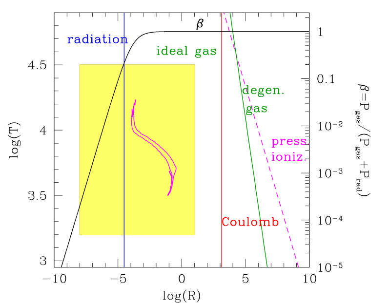
Figure 1: Location of our RM opacity tables in the $\log(T)-\log(R)$ diagram (shaded rectangular area), together with the approximate boundaries between regions where the total pressure is dominated by different effects: radiation pressure, ideal gas, electron-degenerate gas, Coulomb interactions, and pressure ionisation. The vertical line to the left of which radiation dominates the pressure is given by $P_{\rm gas}=P_{\rm rad}$ with $\mu=0.5$. Along the border line between the ideal and degenerate gas we equate the corresponding pressures of a non-relativistic electron gas with mean molecular weight $\mu_{e}=2$. The vertical boundary at $\log(R)\sim 3$, beyond which the Coulomb coupling of charged particles should become important, is defined by the condition $\Gamma_{\rm C}=1$, where $\Gamma_{\rm C}=1.1\,10^{-5}T/\rho^{1/3}$ is the Coulomb coupling parameter for an ionised-hydrogen plasma. Pressure ionisation is assumed to become dominant at $\log(\rho)=0$ for $\log(T)\leq 4.5$, a typical value according to the analysis developed by Luo (1997). The behaviour of the parameter $\beta$ (defined in the text) is also shown. As an example, the evolution of the photospheric parameters ($T_{\rm eff},\,R_{\rm phot}$) of a stellar model with initial mass $M=5\,M_{\odot}$, and metallicity $Z=Z_{\rm ref}=0.02$ is depicted by a magenta line, covering the evolution from the pre-main sequence to the first pulses on the TP-AGB (calculations performed with the Padova stellar evolution code).

3.1 State variables

Under the assumption of ideal gas, described by the law

$$P_{\rm gas}=\displaystyle\frac{k_{\rm B}}{\mu m_{\rm u}}\rho T\,,$$ (29)

one must specify one pair of independent state variables. Usual choices are, for instance, $(P_{\rm gas},T)$ or $(\rho,T)$. For practical and historical reasons, opacity tables are generally built as a function of the logarithm of the temperature $T$, and the logarithm of the $R$ variable, defined as $R=\rho/(T_{6})^{3}$, with $T_{6}=T/(10^{6}\,{\rm K})$.

An advantage of using the $R$ parameter, instead of $\rho$ or $P$, is that the opacity tables can cover rectangular regions of the $(R,\,T)$-plane, without the nasty voids over extended temperature ranges that would come out if intervening changes in the EOS are not taken into account (e.g. transition from ideal to degenerate gas).

Interestingly, as pointed out by Mayer & Duschl (2005; see their appendix D), different $R$ values correspond to different gas/radiation pressure ratios, $\delta=P_{\rm gas}/P_{\rm rad}$. The relation between $\log(R)$ and $\log(\delta)$ is linear, with larger $R$ values corresponding to larger $\delta$, i.e. an increasing importance of $P_{\rm gas}$ against $P_{\rm rad}$. Moreover, we notice that the equality $P_{\rm gas}=P_{\rm rad}$ takes place in the range at $-4.8\la\log(R)\la-4.5$, assuming a mean molecular weight varying in the interval $0.5\la\mu\la 1$. In Fig. 1 we also plot the quantity $\beta=P_{\rm gas}/(P_{\rm gas}+P_{\rm rad})$, a parameter frequently used by stellar evolutionists.

In this respect Fig. 1 illustrates the rectangular region covered by our RM opacity tables in the $\log(T)-\log(R)$ diagram, defined by the intervals $(3.2\leq\log(T)\leq 4.5)$ and $(-8\leavevmode\nobreak\ \leq\leavevmode\nobreak\ \log(R)\leavevmode\nobreak\ \leq\leavevmode\nobreak\ 1)$. We note that the table area lies in the domain of the ideal gas, and it extends into the region dominated by radiation pressure for $\log(R)\leq-4.5$. Non ideal effects related to electron degeneracy, Coulomb coupling of charged particles, and pressure ionisation of atoms are expected to become dominant outside the table boundaries, in the domain of high-density plasmas.

It is important to remark that our RM opacity tables can be easily extended to higher temperatures, $\log(T)>4.5$, with the RM opacity data provided by OPAL and OP. As a matter of fact the agreement between our results and OPAL is good in the overlapping transition region, say $3.9\la\log(T)\la 4.5$ (see Sect. 4.1.1 and panel c) of Fig 7).

Within the aforementioned limits of the state variables, the interactive web mask enables the user to freely specify the effective ranges of $\log(T)$ and $\log(R)$ of interest as well as the spacing of the grid points $\Delta\log(T)$ and $\Delta\log(R)$. From our tests it turns out that a good sampling of the main opacity features can be achieved with $\Delta\log(T)=0.05$ for $\log(T)>3.7$ and $\Delta\log(T)=0.01$ for $\log(T)\leq 3.7$, and $\Delta\log(R)=0.5$. In any case, the choice should be driven by consideration of two aspects, i.e. maximum memory allocation, and accuracy of the adopted interpolation scheme.

3.2 Chemical composition

It is specified in terms of the following quantities:

• The reference solar mixture;

• The reference metallicity $Z_{\rm ref}$;

• The hydrogen abundance $X$;

• The reference mixture;

• The enhancement/depression factor $f_{i}$ of each element (heavier than helium), with respect to its reference abundance.

The reference solar mixture can be chosen among various options, which are referenced in Table 3. For their relevance to the opacity issue, the corresponding solar metallicity, $Z_{\odot}$, and the $({\rm C/O})_{\odot}$ ratio are also indicated. Scrolling Table 3 from top to bottom we note that $Z_{\odot}$ significantly decreases, passing from $\sim 0.019$ in AG89 down to $\sim 0.012$ in GAS07. This implies that opacity tables constructed assuming the same $Z$ may notably differ depending on the adopted solar mixture. Concerning C/O, a key parameter affecting the opacities for $\log(T)\la 3.5$, we see that it spans a rather narrow range ($0.43\la$ C/O $\la 0.53$) passing from one compilation to the other, except for the H01 which corresponds to a higher value, C/O $\sim 0.72$. How much these differences in the reference solar mixtures may impact on the resulting opacities is discussed in Sect. 4.1.

Reference	$Z_{\odot}$	(C/O)⊙	(C/O)crit,1
Anders & Grevesse 1989 (AG89)	0.0194	0.427	0.958
Grevesse & Noels 1993 (GN93)	0.0173	0.479	0.952
Grevesse & Sauval 1998 (GS98)	0.0170	0.490	0.947
Holweger 2001 (H01)	0.0149	0.718	0.937
Lodders 2003 (L03)	0.0132	0.501	0.929
Grevesse et al. 2007 (GAS07)	0.0122	0.537	0.929
Caffau et al. 2009 (C09)	0.0155	0.575	0.938

Table 3: Compilations of the solar chemical composition adopted in the computation of the EOS and gas opacities. For each mixture the solar total metallicity $Z_{\odot}$ (in mass fraction), the abundance ratios (C/O)_⊙ and (C/O)_crit,1 are indicated for comparison. The latter marks a critical boundary for the gas molecular chemistry in the range $3.2\leavevmode\nobreak\ \leq\leavevmode\nobreak\ \log(T)\leavevmode\nobreak\ \leq\leavevmode\nobreak\ 3.6$. The C and O abundances are expressed as number fractions.

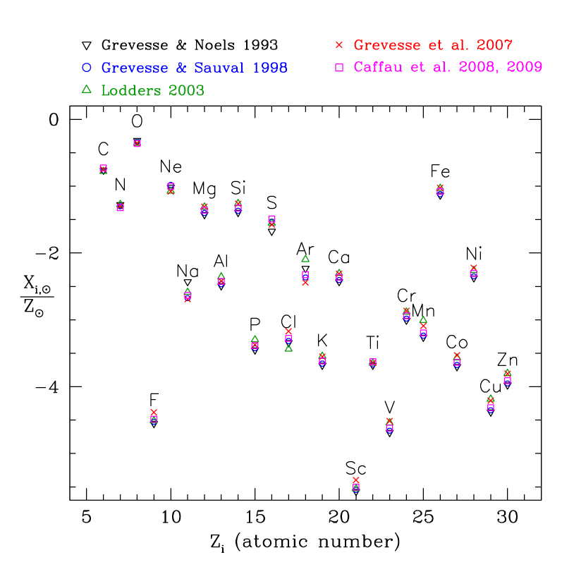
Figure 2: Fractional abundances of elements, with nuclear charge $Z_{i}=6-30$, normalised to the solar metallicity according to various compilations, as indicated.

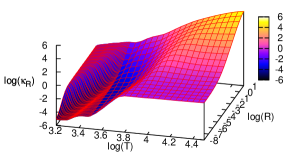
Figure 3: Rosseland mean opacity as a function of variables $T$ and $R$ over the entire parameter space considered in our calculations. The adopted composition is assumed to have $Z=Z_{\rm ref}=0.02$, $X=0.7$ and the metal abundances scaled-solar to the GS98 mixture.

Let us indicate with $\mathcal{N}_{Z}$ the number of metals, i.e. the chemical elements heavier than helium, with atomic number $Z_{i}\geq 3$. Each metal is characterised by an abundance $X_{i}$ in mass fraction and, equivalently, an abundance $\varepsilon_{i}$ in number fraction, respectively defined as:

$$X_{i}=\displaystyle\frac{A_{i}N_{i}}{\sum_{j=1}^{\mathcal{N}_{\rm el}}A_{j}N_{j}}\,\,\,\,\,\,\,{\rm and}\,\,\,\,\,\,\,\varepsilon_{i}=\displaystyle\frac{N_{i}}{N_{\rm a}}=\displaystyle\frac{N_{i}}{\sum_{j=1}^{\mathcal{N}_{\rm el}}N_{j}}\,,$$ (30)

where $N_{i}$ is the number density of nuclei of type $i$ with atomic mass $A_{i}$, and $N_{\rm a}$ is the total number density of all atomic species (with the same notation as in Sect. 2.1.2). In both cases the normalisation condition must hold, i.e. $\sum_{i=1}^{\mathcal{N}_{\rm el}}X_{i}=1$ and $\sum_{i=1}^{\mathcal{N}_{\rm el}}\varepsilon_{i}=1$. The total metal abundance is given by $Z=\sum_{i\geq 3}X_{i}$ in mass fraction, and $\varepsilon_{Z}=\sum_{i\geq 3}\varepsilon_{i}$ in number fraction.

We assign each metal species the variation factors, $f_{i}$ and $g_{i}$, relative to the reference mixture:

$$X_{i}=f_{i}X_{i,{\rm ref}}\,\,\,\,\,\,\,{\rm and}\,\,\,\,\,\,\,\varepsilon_{i}=g_{i}\varepsilon_{i,{\rm ref}}\,.$$ (31)

The reciprocal relations between $X_{i}$ and $\varepsilon_{i}$ derive straightforwardly:

$$X_{i}=\displaystyle\frac{A_{i}\varepsilon_{i}}{\sum_{j=1}^{\mathcal{N}_{\rm el}}A_{j}\varepsilon_{j}}\,\,\,\,\,\,\,{\rm and}\,\,\,\,\,\,\,\varepsilon_{i}=\displaystyle\ \frac{X_{i}/A_{i}}{\sum_{j=1}^{\mathcal{N}_{\rm el}}X_{j}/A_{j}}\,\,,$$ (32)

as well as those between $f_{i}$ and $g_{i}$ for metals:

$$f_{i}=g_{i}\,\displaystyle\frac{\sum_{j\geq 3}A_{j}\varepsilon_{j}^{\rm ref}}{\sum_{j\geq 3}A_{j}\varepsilon_{j}}\,\,\,\,\,\,\,{\rm and}\,\,\,\,\,\,\,g_{i}=f_{i}\,\displaystyle\frac{\sum_{j\geq 3}X_{j}^{\rm ref}/A_{j}}{\sum_{j\geq 3}X_{j}/A_{j}}\,.$$ (33)

We have verified that $f_{i}\approx g_{i}$ as long as they are not too large and the ratios between the two summations in the left-hand side members of Eq. (33) do not deviate significantly from unity (see, for instance, Table 4).

In principle, the reference chemical mixture can be any given chemical composition. Frequent choices are, for instance, mixtures with scaled-solar partitions of metals, or with enhanced abundances of $\alpha$-elements. The ÆSOPUS code is structured to allow large freedom in specifying the reference mixture. For simplicity, in the following we will adopt the solar mixture as the reference composition, so that the reference metal abundances are

$$X_{i,{\rm ref}}=X_{i,{\odot}}\displaystyle\frac{Z}{Z_{\odot}}\,\,\,\,\,\,\,{\rm and}\,\,\,\,\,\,\,\varepsilon_{i,{\rm ref}}=\varepsilon_{i,{\odot}}\displaystyle\frac{\varepsilon_{Z}}{\varepsilon_{Z_{\odot}}}$$ (34)

with clear meaning of the symbols. The partitions, $X_{i,{\odot}}/Z_{\odot}$, of chemical elements from C to Zn are shown in Fig. 2 for a few compilations of the solar chemical composition.

According to the notation presented by Annibali et al. (2007), the chemical elements can be conveniently divided into three classes depending on the sign of $f_{i}$ (or $g_{i}$) , namely:

• enhanced elements with $f_{i}>1$ (or $g_{i}>1$);

• depressed elements with $f_{i}<1$ (or $g_{i}<1$);

• fixed elements with $f_{i}=1$ (or $g_{i}=1$).

The latter correspond to the reference abundances, i.e. scaled-solar in the case discussed here. Moreover, let us designate

• selected elements with $f_{i}\neq 1$ (or $g_{i}\neq 1$)

the group of elements which are assigned variation factors different from unity (either enhanced or depressed), as part of the input specification. We limit the discussion here to the case of the abundances $X_{i}$ expressed in mass fraction, since exactly the same scheme, with the due substitutions, can be applied to the abundances $\varepsilon_{i}$ in number fraction. In this respect one should bear in mind that the conversions $X_{i}\rightleftarrows\varepsilon_{i}$ are obtained with Eqs. (32). Starting from the reference mixture, then the new mixture can be obtained in two distinct ways:

1. Case $Z\neq Z_{\rm ref}$. The enhancement/depression factors $f_{i}$ of the selected elements produce a net increase/depletion of total metal content relative to the reference metallicity $Z_{\rm ref}$. The actual metallicity is calculated directly with $Z=\sum_{i=1}^{\mathcal{N}_{Z}}f_{i}X_{i,{\rm ref}}$. In this case all $\mathcal{N}_{Z}$ variation factors $f_{i}$ can be freely specified without any additional constrain.

2. Case $Z=Z_{\rm ref}$. The enhancement/depression factors produce non-scaled-solar partitions of metals, while the total reference metallicity $Z_{\rm ref}$ is to be preserved. This constraint can be fulfilled with various schemes, e.g. by properly varying the total abundance of all other non-selected elements so as to balance the abundance variation of the selected group. For instance, if the selected elements have all $f_{i}>0$, so that we refer to them as enhanced group, then the whole positive abundance variation should be compensated by the negative abundance variation of the complementary depressed group. Another possibility is to define a fixed group of elements whose abundances should not be varied, hence not involved in the balance procedure; in this case the preservation of the metallicity is obtained by properly changing the abundances of a lower number of atomic species among the non-selected ones.

   In principle, the quantities $f_{i}$ can be chosen independently for up to a maximum of $(\mathcal{N}_{Z}-1)$ elements, while the remaining factor is bound by the $Z=Z_{\rm ref}$ condition. A simple practise is to assign the same factor to all the elements belonging to the selected group, either enhanced or depressed, as frequently done for $\alpha$-enhanced mixtures. In this respect more details can be found in Sect. 4.3.

The former case ($Z\neq Z_{\rm ref}$) properly describes a chemical mixture in which the abundance variations are the product of nuclear burnings occurring in the stellar interiors. This applies, for instance, to thermally-pulsing asymptotic giant branch (TP-AGB) stars whose envelope chemical composition is enriched in C and O produced by He-shell flashes and convected to the surface by the third dredge-up, which leads to an effective increment of the global metallicity $(Z>Z_{\rm ref})$.

The latter case ($Z=Z_{\rm ref}$) corresponds, for instance, to chemical mixtures with a scaled-solar abundance of CNO elements $X_{\rm CNO}$, but different ratios e.g. $X_{\rm C}/X_{\rm CNO}$, $X_{\rm N}/X_{\rm CNO}$, and $X_{\rm O}/X_{\rm CNO}$. Alternatively, if we consider the abundances in number fractions, the condition, $\varepsilon_{\rm CNO}=$ const., may describe the surface composition of an intermediate-mass star after the second dredge-up on the early AGB, when products of complete CNO-cycle are brought up to the surface. In this case the total number of CNO catalysts does not change, while C and O have been partly converted to ¹⁴N. Another example may refer to $\alpha$- enhanced mixtures with different [$\alpha$/Fe]$>0$ but the same metal content $Z$.

Finally, it should be noticed that, once the actual metallicity $Z$ is determined, in both cases the normalisation condition implies that the helium abundance is given by the relation $Y=1-X-Z$.

4 Results

In the following sections we will discuss a few applications of the new opacity calculations, selecting those ones that may be particularly relevant in the computation of stellar models. For completeness, our results are compared with other opacity data available in the literature.

4.1 Scaled-solar mixtures

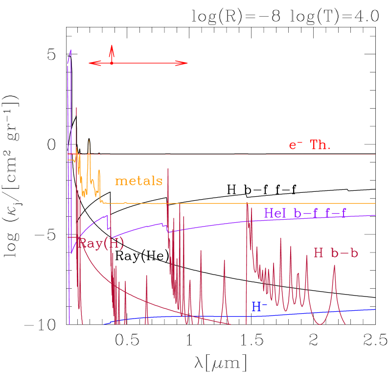
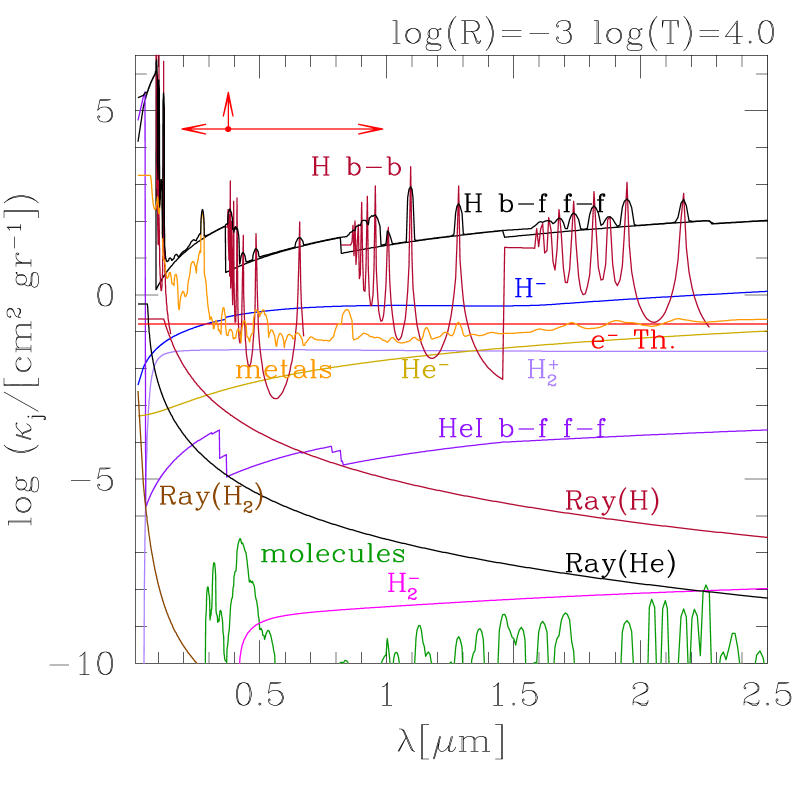
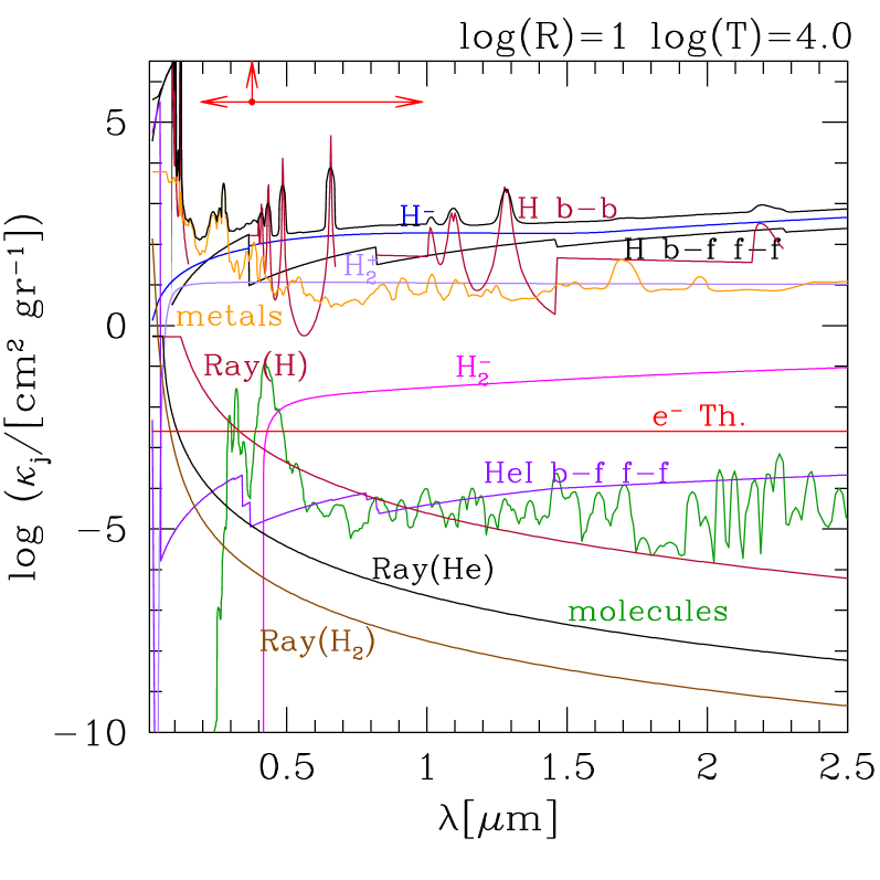
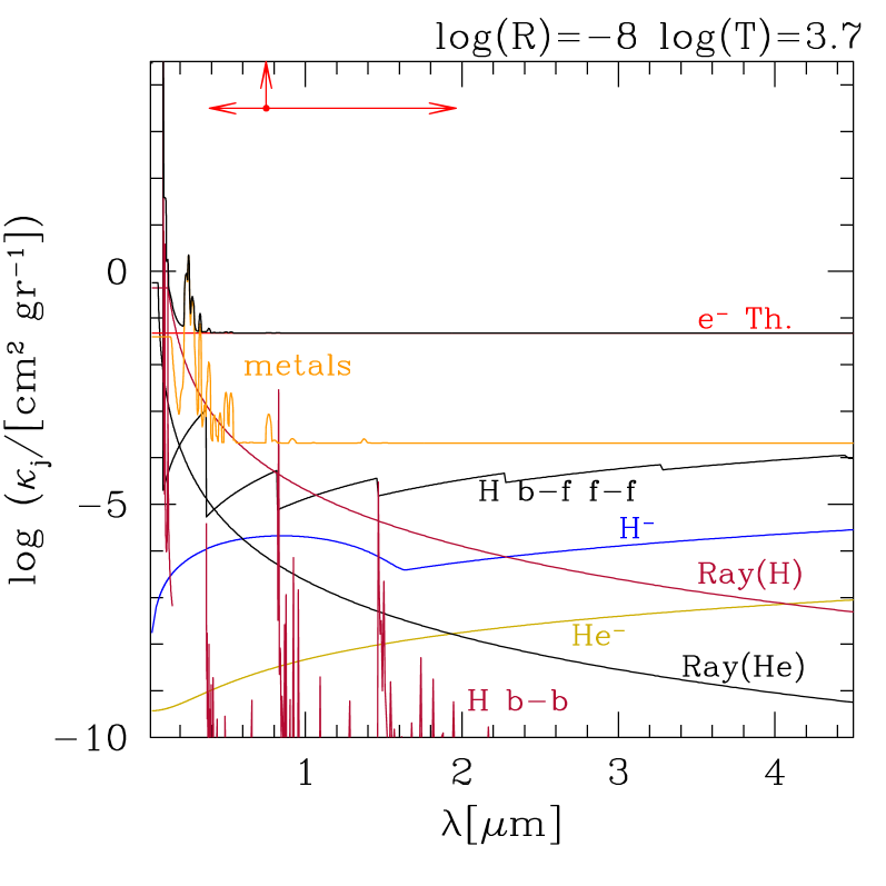
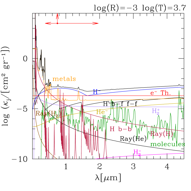
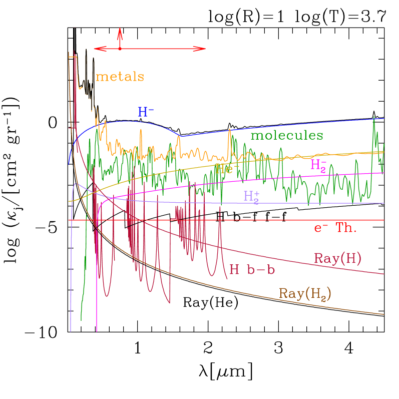
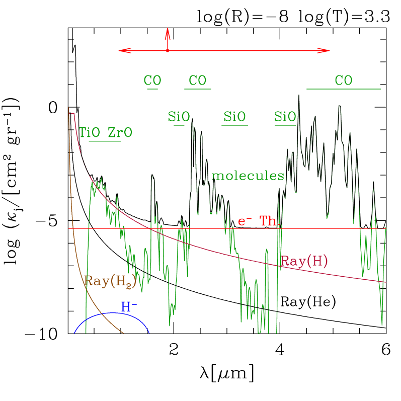
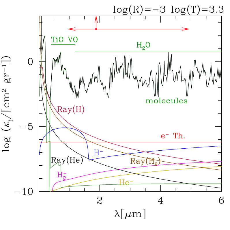
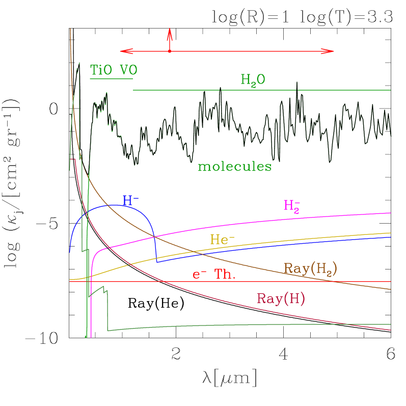
Figure 4: Monochromatic absorption coefficients for several opacity sources as a function of the wavelength, for three values of the temperature and three values of the $R$ variable, as indicated. The chemical composition is defined by $Z=Z_{\rm ref}=0.02$, $X=0.7$ with metal abundances scaled-solar to the GAS07 mixture. The total coefficient is depicted by the highest black line. The vertical arrow marks the wavelength of the maximum of the Rosseland weighting function (given by Eq.28), while the horizontal arrows delimit the wavelength range within which the Rosseland weighting function drops by a factor $1/e$. Where molecular absorption bands are important, the corresponding spectral intervals are also indicated. For graphical purpose only, line absorption coefficients for molecules and atoms are smoothed by convolution with a Gaussian function. The variance is empirically chosen to depend on the wavelength so as to have a neat representation without missing important spectral details.

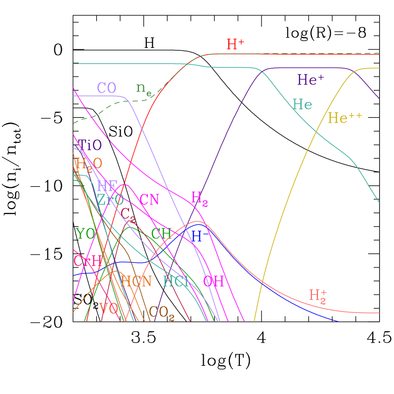
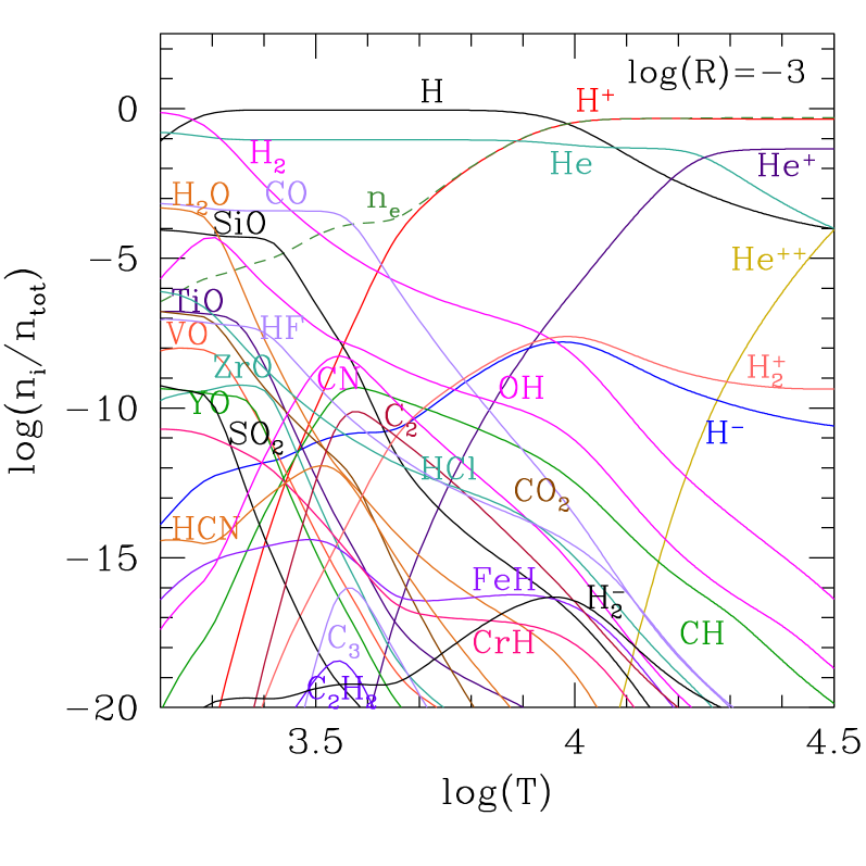
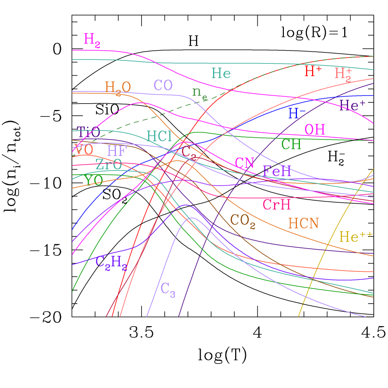
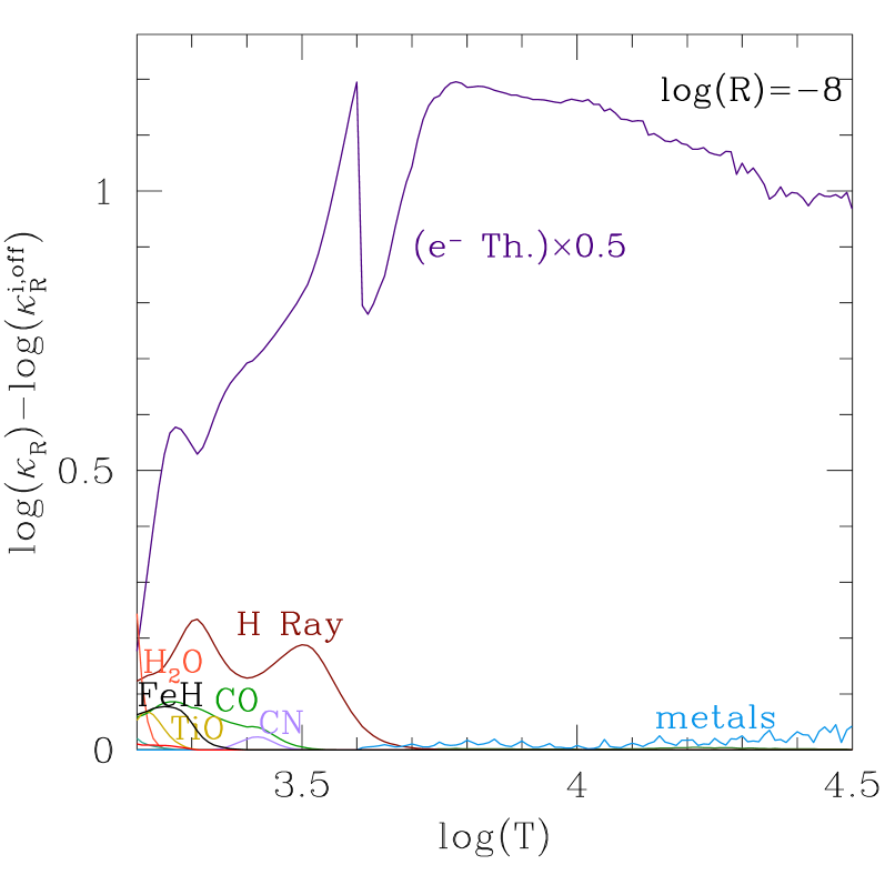
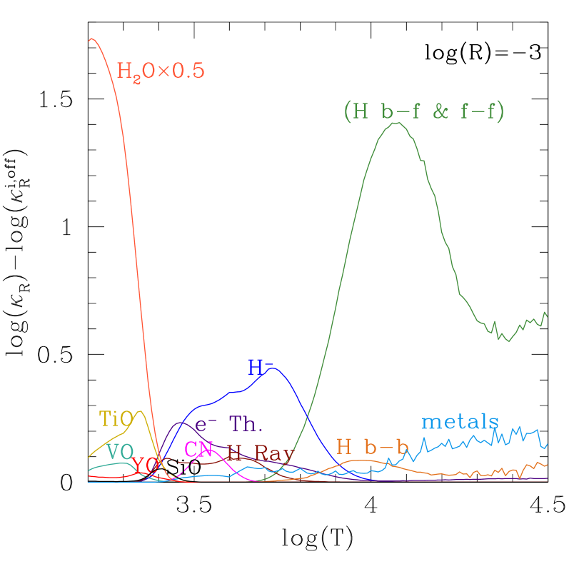
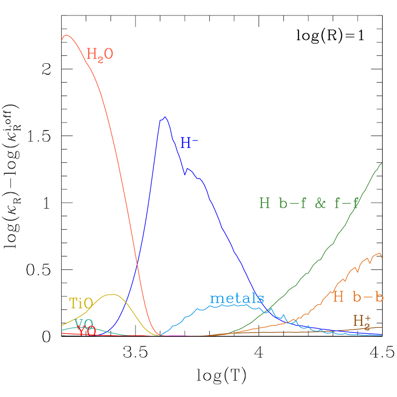
Figure 5: Top panels: concentrations of various chemical species as a function of temperature, for three values of the $R$ parameter, as indicated. Bottom panels: contributions of different opacity sources (both continuous and line-absorption processes) to the total RM opacity. Each curve corresponds to $\log(\kappa)-\log(\kappa_{j}^{\rm off})$, where $\kappa$ is the full opacity including all opacity sources here considered, whereas $\kappa_{j}^{\rm off}$ is the reduced opacity obtained omitting one particular source at once (labelled nearby). The logarithmic notation allows to highlight the temperature domains which characterise the different opacity contributors. The adopted chemical composition consists of $X=0.7$, $Z=Z_{\rm ref}=0.02$, with elemental abundances scaled according to the GAS07 solar mixture.

Let us first illustrate the case of scaled-solar mixtures, which will serve as reference for other compositions. As an example, Fig. 3 visualises the tri-dimensional plot of one opacity table calculated over the whole $\log(T)-\log(R)$ parameter space for a given chemical mixture. The latter is characterised by ($X=0.7$; $Z_{\rm ref}=0.02$; $Z=Z_{\rm ref}$; $f_{i}=1$, for $i=3\cdots N_{\rm el}$) according to the notation introduced in Sect. 3, meaning that all metal abundances are scaled-solar. One can see that the grid of the state variables (i.e. $\Delta\log(T)=0.01$ for $3.2\leq\log(T)\leq 3.5$, and $\Delta\log(T)=0.05$ for $3.5<\log(T)\leq 4.5$; $\Delta\log(R)=0.5$) is sufficiently dense to allow a smooth variation of $\kappa_{\rm R}$ all over the parameters space, which is a basic requirement for accurate interpolation.

Different opacity sources dominate the total $\kappa_{\rm R}$ in different regions of the $\log(T)-\log(R)$ plane. Roughly speaking, we may say that the continuous and atomic opacities prevail at higher temperatures, while molecular absorption plays the major rôle for $\log(T)\la 3.5$. It has been known for long time (see e.g. Alexander 1975), for instance, that the prominent opacity bump peaking at $\log(T)=\sim 3.25$ in Fig. 6 is mainly due to the strong absorption of H₂O molecular bands. To delve deeper into the matter it is instructive to look at Fig. 4 and Fig. 5, which illustrate the basic ingredients affecting the RM opacity and their dependence on wavelength, temperature and density.

Figure 4 displays the spectral behaviour of the monochromatic opacity coefficient per unit mass, $\kappa_{j}(\nu)$, of several absorption and scattering processes, as defined by Eqs. (19)–(20). We consider three representative values of the temperature (i.e. $\log(T)=3.3,\,3.7,\ 4.0$) and three choices of the $R$ variable (i.e. $\log(R)=-8,\,-3,\ 1$), for a total of nine panels that should sample the main opacity domains. For each temperature, we also indicate in Fig. 4 the spectral range most relevant for the Rosseland mean, by marking the wavelength, $\lambda_{\rm max}$, at which the Rosseland weighting function reaches its maximum value (given by Eq. 28), and the interval across which it decreases by a factor $1/e$.

At larger temperatures, i.e. $\log(T)=4.0$ and $\lambda_{\rm max}\sim 0.38\,\mu$m (top panels), the total monochromatic coefficient is essentially determined by the Thomson e^- scattering at very low gas densities (see the top-left panel for $\log(R)=-8$), while the H opacity (bound-bound, bound-free, and free-free transitions) plays the major rôle at large $\rho$. Next to hydrogen, some non-negligible contribution comes from atomic absorption at shorter wavelengths.

At intermediate temperatures, i.e. $\log(T)=3.7$ and $\lambda_{\rm max}\sim 0.75\,\mu$m (middle panels), Thomson e^- scattering again controls the total absorption coefficient at the lowest densities, whereas at increasing $\rho$ the most significant opacity sources are due to metals and H^- absorption (electron photo-detachment for $\lambda<1.644\,\mu$m and free-free transitions).

At lower temperatures, i.e. $\log(T)=3.3$ and $\lambda_{\rm max}\sim 1.88\,\mu$m (bottom panels), the molecular absorption bands (mainly of H₂O, VO, TiO, ZrO, CO) dominate the total absorption coefficient at any gas density except for very low values, where the spectral gaps between the molecular bands are filled in with the Thomson e^- scattering coefficient. Due to its harmonic character, the Rosseland mean opacity emphasises just these opacity holes, so that the total $\kappa_{\rm R}$ for $\log(T)=3.3$ and $\log(R)=-8$ will be mostly determined by the Thomson e^- scattering, with a smaller contributions from molecules.

This fact becomes more evident with the help of Fig. 5, which provides complementary information on both the chemistry of the gas, and the characteristic temperature windows of different opacity sources. Results are presented as a function of temperature for three values of the parameter $R$.

As for the chemistry (top panels of Fig. 5), we show the concentrations of a few species, selecting them among those that are opacity contributors, while leaving out all other chemicals to avoid over-crowding in the plots (we recall that ÆSOPUS solves the chemistry for $\mathcal{N}_{\rm tot}\approx 800$ species). It is useful to remark a few important features, namely: i) at lower temperatures molecular formation becomes more efficient at increasing density, ii) the most abundant molecule is either carbon monoxide (CO) thanks to its high binding energy at low and intermediate densities, or molecular hydrogen (H₂) at higher densities; iii) the electron density $n_{e}$ is essentially supplied by H ionisation down to temperatures $\log(T)\simeq 3.8-3.6$, below which the main electrons donors are nuclei with low-ionisation potentials, such as: Mg, Al, Na, Si, Fe, etc. (see Fig. 22 and Sect. 4.3 for more discussion of this point).

The bottom panels display the contributions of several absorption/scattering processes to the total RM opacity. This is done by considering, for a given source $j$, the ratio $\kappa_{j}^{\rm off}/\kappa_{\rm R}$, where $\kappa_{j}^{\rm off}$ is the reduced RM opacity obtained by including all opacity sources but for the $j^{\rm th}$ itself.

At very low densities, i.e. $\log(R)=-8$ (left-hand side panel of Fig. 5) the most important opacity source, all over the temperature range under consideration, is by far Thomson scattering from free electrons. Note that at lower temperatures a relatively important contribution is provided by Rayleigh scattering from neutral hydrogen, while the rôle of molecules is marginal since at these low densities molecular formation is inefficient.

Different is the case with $\log(R)=-3$ (middle panel of Fig. 5). We can distinguish three main opacity domains as a function of temperature. At lower temperatures, say for $3.2\la\log(T)\la 3.6$, molecules completely rule the opacity, with H₂O being the dominant source for $\log(T)\la 3.4$. Additional modest contributions come from metal oxides, such as TiO, VO, YO, and SiO. Note that, though for C/O $<1$ the chemistry is dominated by O-bearing molecules, there is a small opacity bump due to CN at $\log(T)\approx 3.5$. At intermediate temperatures, $3.6\la\log(T)\la 3.8$, the most important rôle is played by the H^- continuum opacity, which in turn depends on the availability of free electrons supplied by ionised metals. Additional opacity contributions are provided by Thomson scattering from electrons and Rayleigh scattering from neutral hydrogen. At larger temperatures, $3.8\la\log(T)\la 4.5$, the total RM opacity is determined mostly by the b-f and f-f continuous absorption from hydrogen, with further contributions from b-b transitions of H and atomic opacities.

In the high density case with $\log(R)=1$ (right-hand side panel of Fig. 5), the opacity pattern is similar to the one just described, with a few differences. The most noticeable ones are the sizable growth of the H^- opacity bump in the intermediate temperature window, and the increased importance of the H lines at higher temperatures.

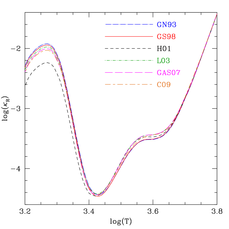
Figure 6: Rosseland mean opacity as a function of temperature and assuming $\log R=-3$. The adopted chemical composition consists of $X=0.7$, $Z=Z_{\rm ref}=0.02$, with elemental abundances scaled according to a few compilations of the solar mixture abundances, namely: Grevesse & Noels 1993; Grevesse & Sauval 1998; Holweger 2001; Lodders 2003; Grevesse, Asplund & Sauval 2007; Caffau et al. (2008, 2009). Note the significant depression of the H₂O bump in the Holweger (2001) case compared to the others, due to the lower oxygen abundance, hence (C/O)_⊙ ratio.

Finally, we close this section by examining the sensitiveness of the RM opacity to the underlying reference solar mixture. Figure 6 shows an example of our opacity calculations made adopting a few solar abundances compilations available in the literature. They are summarised in Table 3. The largest differences are expected for $\log T\la 3.4$, where the RM opacity is dominated by the opacity bump caused by the H₂O molecule, whose amplitude is extremely sensitive to the excess of oxygen with respect to carbon, hence to the C/O ratio. In fact, we notice that the opacity curves corresponding to GN93, GS98, L03, GAS07, and C09 lie rather close one to each other, just reflecting the proximity of their C/O ratios ($\approx 0.5-0.6$; see Table 3). For the same reason, the RM opacity predicted at $\log T\sim 3.3$ with the H01 solar mixture is roughly 50$\%$ lower, given the higher C/O ratio ($\approx 0.7$).

Some differences in RM opacity are also expected in the $3.5\la\log(T)\la 3.65$ interval, which is affected mainly by the CN molecular bands and the negative hydrogen ion H^-. We see in Fig. 6 that most of the results split into two curves: the opacities based on L03 and GAS07 (and partly also C09) are higher than those referring to GN93 and GS98 solar mixtures. In this case the differences are not caused by the CN molecule, but rather reflect the differences in the electron density. As one can notice in Fig. 2, L03, GAS07 (and C09) compilations correspond to higher solar partitions, $X_{i,\odot}/Z_{\odot}$, of those elemental species that mostly provide the budget of free electrons at these temperatures, such as: Mg, Si, Ca, and Fe (see also Fig. 22). As a consequence, the H^- opacity is strengthened in comparison to the GN93 and GS98 cases. On the other hand, the opacity curve corresponding to the H01 mixture lies somewhere in the middle. This is the indirect result of the larger C/O ratio (i.e. more carbon is available) which favours a larger concentration, hence opacity contribution, of the CN molecule in this temperature window.

The arguments developed here indicate that the expression “standard solar composition” should be always specified explicitly together with its reference compilation and not taken for granted, since significant differences arise in the RM opacities depending on the adopted solar mixture.

4.1.1 Comparison with other authors

As a next step we checked our opacity results against tabulated RM data made publicly available from other authors. In Fig. 7 we show eight representative comparisons, based on: the widely-used and well-tested database set up by the Wichita State University group, i.e. Alexander & Ferguson (1994), Ferguson et al. 2005 (hereafter also F05); the recent data by Lederer & Aringer 2009 (hereafter also LA09) stored in the VizieR service; the RM data available in the Robert L. Kurucz’ homepage, and the OPAL and OP data computed via their interactive web-masks. The $R$ and $T$ intervals are different depending on the source considered. For instance, the comparisons with the OPAL and OP opacities cover the range from $3.8\leq\log(T)\leq 4.5$, since no molecular contribution is included in the OPAL and OP data.

In general we can conclude that the check is quite satisfactory in all cases under examination, as our opacity values agree with the reference data mostly within $\pm 0.05$ dex, with the largest differences reaching up to $\approx\pm 0.10-0.20$ only in narrow regions.

Let us start discussing the comparison with Alexander & Ferguson (1994) and Ferguson et al. (2005), illustrated in panels from a) to d) assuming various reference solar compositions. First we notice that the small magenta areas in the upper-left corners of the four panels are not included in the test, since at those densities and temperatures dust is expected to condensate , whereas our EOS describes the matter in the gas phase.

Besides this, in all cases the agreement between the opacity data of the Wichita State University group and ÆSOPUS is very good for $3.4\leq\log(T)\leq 4.5$, the differences $\Delta\log(\kappa_{R})$ being mostly comprised within $\pm 0.05$ dex throughout the $R$ range. For $\log(T)<3.4$ the deviations between F05 and ÆSOPUS appear to grow with a systematic trend, i.e. $\log(\kappa_{R}^{\rm\AE SOPUS})>\log(\kappa_{R}^{\rm F05})$, at increasing $R$. Anyhow, the variations are not dramatic, the biggest values arriving at $\approx-0.15/-0.20$. This result is not surprising since this is just the region where molecular absorption dominates, so that the predicted RM opacity is sensitive to differences in the treatment of the molecular line opacities (line lists, broadening, adopted frequency grid, etc.).

This applies also when comparing different releases of the same database as it is illustrated, for instance, by panels a) and b) relative to the data of the Wichita State University group. We notice that where ÆSOPUS exhibits the best agreement ($<0.05$ dex) with Alexander & Ferguson (1994) at $\log(T)\approx 3.4$ and $\log(R)\ga-3$, the largest differences ($0.15-0.20$ dex) show up instead in the comparison with F05 for the same set of abundances. In this respect, we expect that much of the discrepancy between F05 and ÆSOPUS for $3.2\leq\log(T)\leq 3.4$ is due to the different molecular line data adopted for water vapour, i.e. Partridge & Schwenke (1997) and Barber et al. (2006), respectively.

Support to the above interpretation is found when comparing panel c) and e), the latter showing the check of ÆSOPUS results against Lederer & Aringer (2009) for the L03 solar mixture. As we see the agreement here is quite fair all over the $\log(T)-\log(R)$ diagram, even in the low-$T$ corner dominated by H₂O, VO, and TiO absorption, where larger differences with F05 (panel c) arise. As a matter of fact, in ÆSOPUS we adopt essentially the same molecular data as in LA09, so that a good match is in principle expected.

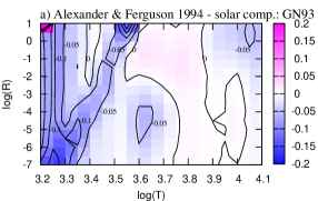
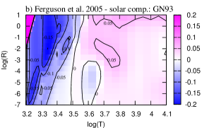
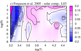
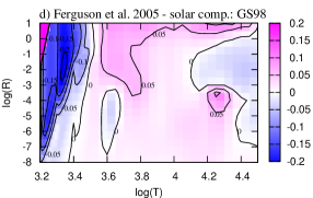
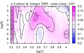
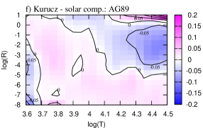
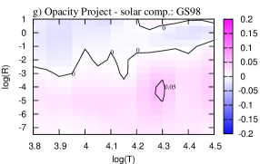
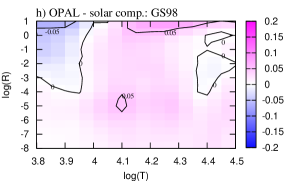
Figure 7: Comparison between our RM opacity results and those provided by other authors, in terms of $\log(\kappa_{\rm R}^{\rm author})-\log(\kappa_{\rm R}^{\rm\AE SOPUS})$. Contour lines, with an incremental step of $0.05$ dex, are superimposed to guide the eye. In all cases, except for Kurucz , the adopted chemical composition corresponds to $Z=Z_{\rm ref}=0.02$, $X=0.7$. External data are taken from: Alexander & Ferguson (1994) and Ferguson et al. (2005) adopting the Grevesse & Noels (1993) solar mixture (panels a and b); Ferguson et al. (2005) assuming the solar abundances from Lodders (2003) (panel c) and Grevesse & Sauval (1998) (panel d); Lederer & Aringer (2009) adopting the Lodders (2003) solar mixture (panel e); Kurucz’ web database for a chemical composition with $Z=Z_{\odot}=0.0194$, $X=X_{\odot}=0.7065$ according to the Anders & Grevesse (1989) solar mixture (panel f); OP and OPAL assuming the Grevesse & Sauval (1998) solar mixture (panels g and h).

Finally, let us briefly comment on the bottom panels (g and h) of Fig. 7, relative to two data sets, OP and OPAL, which are widely used to describe the RM opacity of the gas in the high-T regions, say for $\log(T)>4.0$. The comparison with ÆSOPUS in the overlapping interval, $3.8\leq\log(T)\leq 4.5$, is really excellent, so that the OP and OPAL opacity tables may be smoothly complemented in the low-$T$ regime with ÆSOPUS calculations.

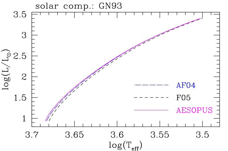
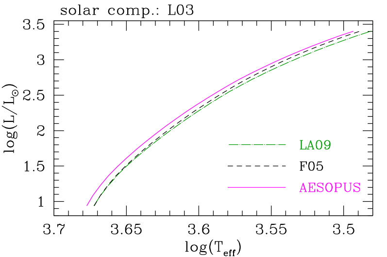
Figure 8: Predicted RGB tracks described by a $1.5\,M_{\odot}$ model with $Z=0.02,\,X=0.7$ and scaled-solar abundances of metals according to either GN93 (left panel) or L03 (right panel). The luminosity is derived from the core-mass luminosity relation given by Boothroyd & Sackmann (1988), while increasing the core mass from $0.20\,M_{\odot}$ to $0.45\,M_{\odot}$. The effective temperature is the result of envelope integrations (see the text for more details). The different curves correspond to RM opacity tables computed by different authors, in the temperature range $3.2\,\leq\log(T)\leq 4.0$.

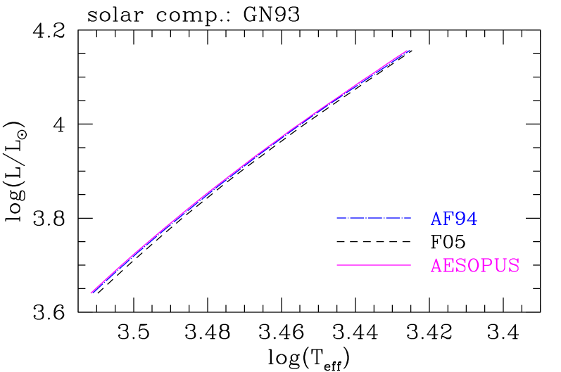
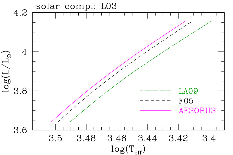
Figure 9: Predicted AGB tracks described by a $2.0\,M_{\odot}$ model with $Z=0.02,\,X=0.7$ and scaled-solar abundances of metals according to either GN93 (left panel) or L03 (right panel). The luminosity is derived from the core-mass luminosity relation, at the quiescent stage of the pre-flash maximum, given by Wagenhuber & Groenewegen (1998), while increasing the core mass from $0.50\,M_{\odot}$ to $0.75\,M_{\odot}$. The effective temperature is the result of envelope integrations (see the text for more details). The different curves correspond to different RM opacity tables, in the temperature range $3.2\,\leq\log(T)\leq 4.0$.

4.1.2 Tests with stellar models

The numerical differences in $\kappa_{\rm R}$ between different authors, illustrated in previous Sect. 4.1.1, assume a physical meaning when one analyses their impact on the models in which the Rosseland mean opacities are employed. As already mentioned in Sect. 1, the largest astrophysical use of pre-tabulated $\kappa_{\rm R}(\rho,\,T)$ is in the field of stellar evolution models to describe, in particular, the thermodynamic structure of the most external layers including the atmosphere.

While it is beyond the scope of this paper to perform a detailed analysis of the effects of low-$T$ opacities on stellar structure and evolution, we consider here two illustrative cases, i.e. the predicted location in the H-R diagram of the Hayashi tracks described by low-mass stellar models while evolving through the RGB and AGB phases. To investigate the differences in $T_{\rm eff}$ brought about by different choices of low-$T$ opacity tables, we have carried out numerical integrations of a complete envelope model (basically the same as the one included in the Padova stellar evolution code) which extends from the atmosphere down to surface of the degenerate core. The overall numerical procedure is fully described in Marigo et al. (1996, 1998), and Marigo & Girardi (2007), so that it will not be repeated here. The mixing-length parameter is assumed $\alpha=1.68$.

As a matter of fact, it has long been known that the atmospheric opacity is critical in determining the position in the H-R diagram of a red-giant star (e.g. Keeley 1970; Scalo & Ulrich 1975). We also recall that during the quiescent burning stages of both RGB and AGB phases of a low-mass star the stellar luminosity is essentially controlled by the mass of the central core (and the chemical composition of the gas), being largely independent of the envelope mass. Adopting suitable core-mass luminosity relations available in the literature, for given value of the core mass and chemical composition, envelope integrations yield the effective temperature at the corresponding luminosity. We have repeated this procedure increasing the core mass – from $0.2\,M_{\odot}$ to $0.46\,M_{\odot}$ for the RGB and from $0.5\,M_{\odot}$ to $0.75\,M_{\odot}$ for the AGB – and adopting different opacity tables for $T\leq 10\,000$ K.

The results for $1.5\,M_{\odot}$ and $2.0\,M_{\odot}$ models with $Z=0.02,\,X=0.7$ are shown in Figs. 8 and 9 for the RGB and AGB tracks respectively. We have adopted low-$T$ opacities from AF94, F05, LA09, and ÆSOPUS, and two reference solar compositions, i.e. GN93 and L03. In all cases the computations with the opacities from ÆSOPUS and from the Wichita State University group are in close agreement, typically being abs$(\log T_{\rm eff}^{\rm AF94}-\log T_{\rm eff}^{\small\rm\AE SOPUS})\la 0.001$ dex (ranging from $\sim 5$ K to $\sim 20$ K) and abs$(\log T_{\rm eff}^{\rm F05}-\log T_{\rm eff}^{\rm\AE SOPUS})\la 0.005$ dex (ranging from $\sim 10$ K to $\sim 50$ K). The deviations from the results with LA09 opacities are somewhat larger, $0.005\la$ abs$(\log T_{\rm eff}^{\rm LA09}-\log T_{\rm eff}^{\rm\AE SOPUS})\la 0.02$ dex (ranging from $\sim 50$ K to $\sim 100$ K). In this respect it should be recalled that in the $T_{\rm eff}$-range considered here, $3.4\la\log(T_{\rm eff})\la 3.7$, the main opacity contributors are the absorption by H^- and Thompson e^- scattering (the concentration of water vapour is still relatively low even at the lowest temperatures; see Fig. 5), so that differences in opacities are likely due to differences in the description of the H^- opacity, and/or in the density of free electrons, which in turn may be affected by differences in the partition functions of the ions with low-ionisation potentials. Anyhow, the temperature differences among the RGB and AGB tracks are in most cases lower than the current uncertainty affecting the semi-empirical $T_{\rm eff}$-scale of F-G-K-M giants ($\sigma\sim 60-80$ K; e.g. Ramírez & Meléndez 2005; Houdashelt et al. 2000).

4.2 Varying C-N-O mixtures

In several situations Rosseland mean opacities for non-scaled solar abundances should be used. One of these cases applies, for instance, to stellar models in which the surface abundances of C, N, and O are altered via mixing and/or wind processes. A remarkable example corresponds to the TP-AGB phase of low- and intermediate-mass stars, whose envelope composition may be enriched with primary carbon (and possibly oxygen) via the third dredge-up, or with newly synthesised nitrogen by hot-bottom burning. As a net consequence, the abundances of C, N, and O as well as their abundance ratios may be significantly changed compared to their pre-TP-AGB values (Wood & Lattanzio 2003). Most critical is the variation of the surface C/O ratio, which controls the chemistry of the gas at the low temperatures typical of the atmospheres of AGB stars (e.g. Marigo 2002).

Indeed, one of the aims of the present work is to provide a flexible computational tool to generate RM opacities for any value of combination of the C-N-O abundances, hence C/O ratio.

Figure 10 shows clearly that big changes in $\kappa_{\rm R}$ are expected at low temperatures, say $\log(T)<3.5$, when passing from an O-rich to a C-rich chemical mixture. For instance, at $\log(T)=3.3$ RM opacities of a gas with C/O$=1.3$ become much larger than in the case with C/O$=0.49$ at lower densities, $-8\la\log(R)\la-3$, while the trend is reversed at increasing density, $\log(R)>-3$. This fact is extremely important for the consequences it brings about to the evolutionary properties of C stars (see e.g. Marigo & Girardi 2007; Cristallo et al. 2007; Marigo et al. 2008; Weiss & Ferguson 2009; Ventura & Marigo 2009).

In this context we will analyse in detail the impact of changing the C/O ratio in a gas mixture, thus simulating the effect of the third dredge-up in TP-AGB stars.

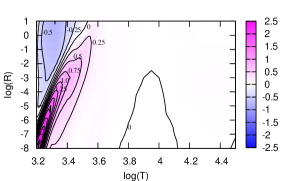
Figure 10: Comparison of RM opacities relative to two gas mixtures with $Z_{\rm ref}=0.02$, $X=0.7$ but different C/O ratios, namely C/O$=1.3$ and C/O$=$C/O${}_{\odot}=0.49$ according to GS98 solar composition. The colour map shows the difference $\log(\kappa_{\rm R}^{{\rm C/O}=1.3})-\log(\kappa_{\rm R}^{{\rm C/O}=0.49})$ throughout the standard location in the $\log(T)-\log(R)$ diagram of one opacity table computed with ÆSOPUS. The contour lines corresponds to differences $\Delta\log(\kappa_{\rm R})$ multiple of $\pm 0.25$ dex. Note the large deviations occurring in the low-$T$ region dominated by molecular absorption.

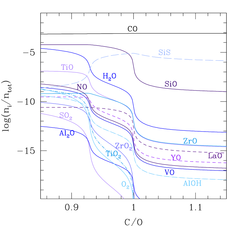
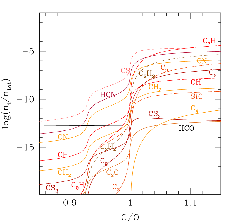
Figure 11: Concentrations of several gas species as a function of the C/O ratio, in a gas mixture with $\log(T)=3.3$, $\log(R)=-3$ (or equivalently $\log(\rho)=-11.1$), $Z_{\rm ref}=0.02$, and $X=0.7$, and adopting the GAS07 reference solar partitions. The increase of C/O follows that of C, while O abundance is kept unchanged. The actual metallicity $Z$ also increases with C. The molecules are divided into two groups, namely: O-bearing molecules (top panel) and C-bearing molecules (bottom panel). Note the sharp change in molecular concentrations at C/O $\approx 1$.

4.2.1 Molecular chemistry: the key rôle of the C/O ratio

Figure 11 illustrates the abrupt change in the chemical equilibria when the C/O ratio passes from below to above unity, in a gas with $\log(T)=3.3$ and $\log(R)=-3$ ($\log(\rho)=-11.1$). From a more careful inspection of Fig. 11 we see that the abundance curves of the O-bearing molecules (top panel) and the C-bearing molecules (bottom panel) follow mirror trends, exhibiting two sudden changes of values at C/O $\approx 0.93$ and C/O $\approx 1.0$. We may say that these two C/O values bracket the transition region between the O-dominated and the C-dominated chemistry. As discussed by Ferrarotti & Gail (2002) the abrupt changes in the chemical equilibria at C/O $\approx 0.93$ and C/O $\approx 1.0$ respectively correspond to the critical values of the carbon abundance

$$\varepsilon_{\rm C}^{{\rm crit},1}=\varepsilon_{\rm O}-\varepsilon_{\rm Si}\,\,\,\longrightarrow\,\,\,{\left(\frac{\rm C}{\rm O}\right)}_{{\rm crit},1} = \frac{\varepsilon_{\rm C}^{{\rm crit},1}}{\varepsilon_{\rm O}}=1-\displaystyle\frac{\varepsilon_{\rm Si}}{\varepsilon_{\rm O}}$$ (35)

$$\varepsilon_{\rm C}^{{\rm crit},2}=\varepsilon_{\rm O}\quad\quad\,\,\,\,\,\longrightarrow\,\,\,{\left(\frac{\rm C}{\rm O}\right)}_{{\rm crit},2} = \frac{\varepsilon_{\rm C}^{{\rm crit},2}}{\varepsilon_{\rm O}}=1$$

The existence of $\varepsilon_{\rm C}^{{\rm crit},1}$ and $\varepsilon_{\rm C}^{{\rm crit},2}$ can be understood considering the extraordinary high bond energies of the two monoxide molecules CO and SiO, i.e. $E_{\rm B}({\rm CO})=11.16$ eV and $E_{\rm B}({\rm SiO})=8.29$ eV, as well as the usually large concentrations of the involved species, i.e. C, O, and to a less extent Si. Following Ferrarotti & Gail (2002) for temperatures $T\la 1\,500$ K, at which dust is expected to condensate, one must also consider the contribution of another strongly-bound molecule, SiS ( $E_{\rm B}({\rm SiS})=6.46$ eV), so that the first critical carbon abundance should be redefined as $\varepsilon_{\rm C}^{{\rm crit},1}=\varepsilon_{\rm O}-\varepsilon_{\rm Si}+\varepsilon_{\rm S}$. Since this study deals with the gas chemistry for $\log(T)\geq 3.2$ (i.e. without dust formation) in the following we limit our discussion to the case described by Eq. (35).

In most cases the bond strength of CO mostly determines the chemical equilibria: as long as $\varepsilon_{\rm C}<\varepsilon_{\rm C}^{\rm crit,1}$, the excess of oxygen atoms, $\varepsilon_{\rm O}-\varepsilon_{\rm C}$, is available for the formation of O-bearing molecules – such as SiO, H₂O, TiO, VO, YO, etc. –, while as soon as $\varepsilon_{\rm C}>\varepsilon_{\rm C}^{\rm crit,2}$, i.e. C/O $>1$, the situation is reversed and the excess of of carbon atoms, $\varepsilon_{\rm C}-\varepsilon_{\rm O}$, takes part in C-bearing molecules such as CN, HCN, C₂, C₂H₂ , SiC, etc. This also explains why, unlike the others, the abundances of the molecules involving the carbon monoxide, like CO itself and HCO, show a flat behaviour with the C/O ratio.

The situation is somewhat different in the transition interval, $\varepsilon_{\rm C}^{\rm crit,1}\la\varepsilon_{\rm C}\la\varepsilon_{\rm C}^{\rm crit,2}$, where the molecular pattern is controlled also by SiO, in addition to CO. The C, O, and Si atoms are now almost completely absorbed in the CO and SiO monoxides, which are the most abundant molecules, as shown in Fig. 11. In other words, the excess of oxygen atoms over carbon is trapped in the molecular bond with silicon, which accounts for the first abundance drop of the other O-bearing molecules at C/O $\simeq 0.93$.

It is clear from Eq. (35) that the value of (C/O)_crit,1 depends on the assumed oxygen and silicon abundances. In principle any change in the ratio ${\rm Si}/{\rm O}$ would correspond to a different (C/O)_crit,1. As a reference case, it is instructive to compare the results for different choices of the solar abundances. They are listed in Table 3. Passing from the AG89 to the most recent GAS07 compilation, the C/O_crit,1 decreases from $\simeq 0.96$ to $\simeq 0.93$, implying that the transition from the O- to the C-dominated chemistry takes place over a wider range of the C/O ratio, i.e. $\sim 0.93-1$ for GAS07 in place of $\sim 0.96-1.00$ for AG89. As we will see later in this section, the knowledge of this critical ratio is of crucial importance since it defines the onset of the transition between two chemical regimes, with consequent dramatic effects on the corresponding RM opacities of the gas (see for instance Figs. 15 and 16).

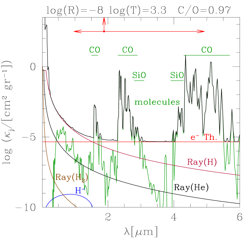
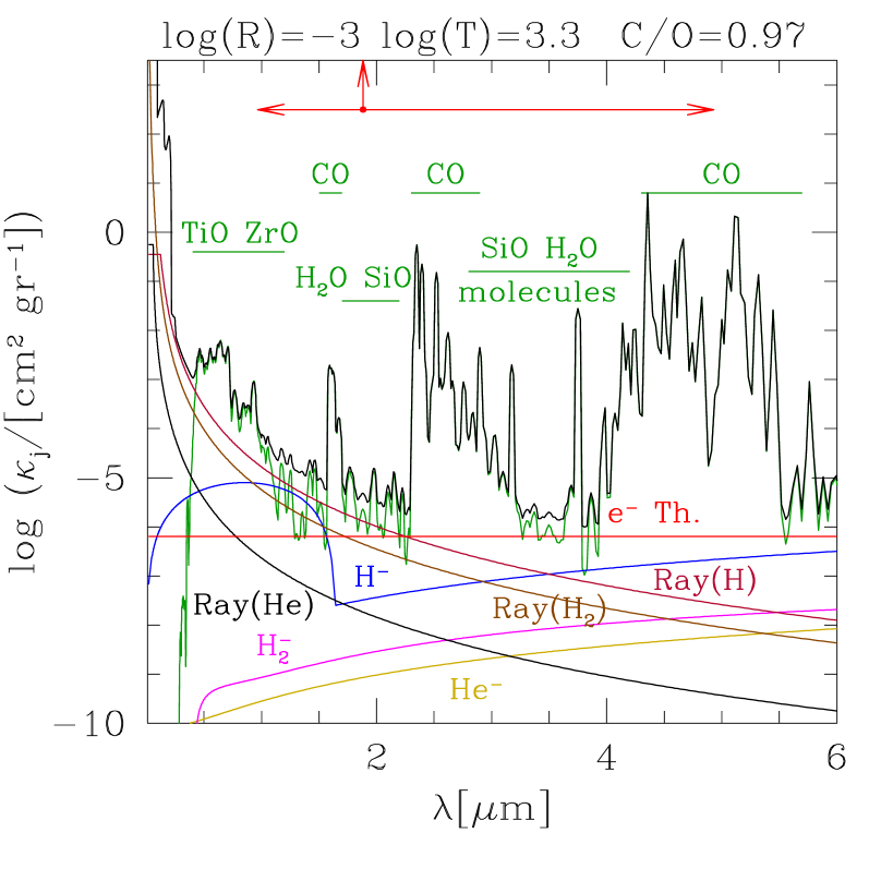
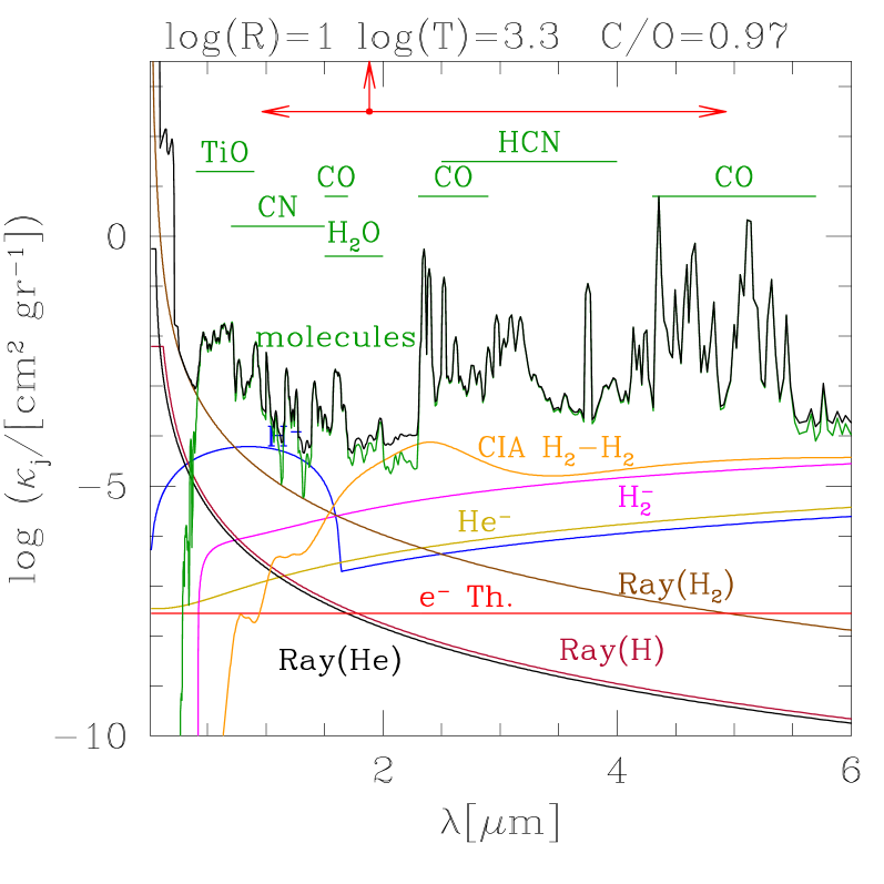
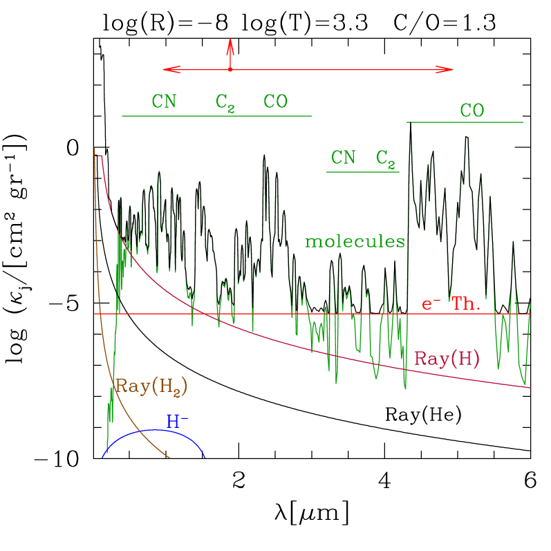
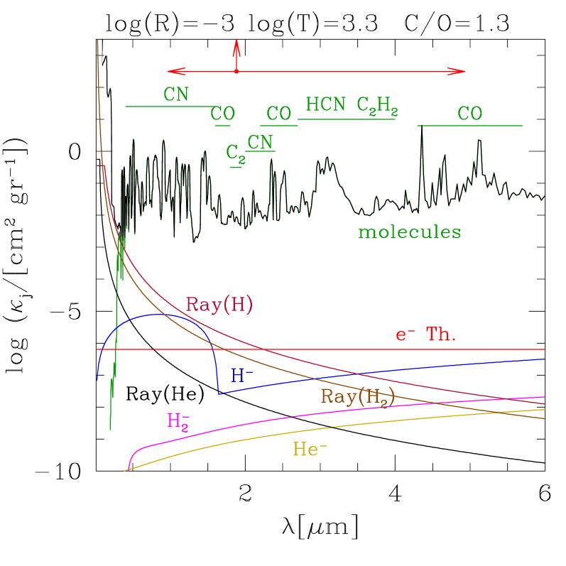
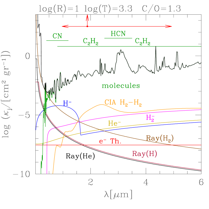
Figure 12: The same as in Fig. 4, but for gas mixtures with C/O=$0.97$ (upper panels) and C/O=$1.30$ (bottom panels) and $\log(T)=3.3$. Note that in the spectral range relevant for the RM opacity, the total monochromatic coefficient is affected by heterogeneous sources (e.g. TiO, ZrO, CO, H₂O, CN, Thomson e^- scattering) for C/O=$0.97$, while absorption by C-bearing molecules dominate for C/O=$1.30$.

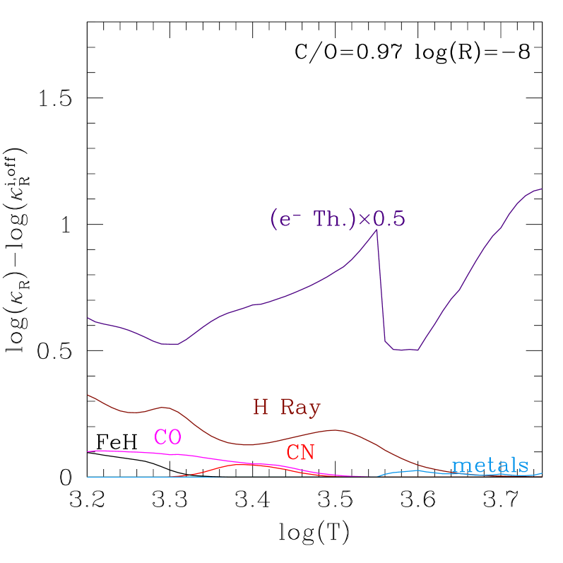
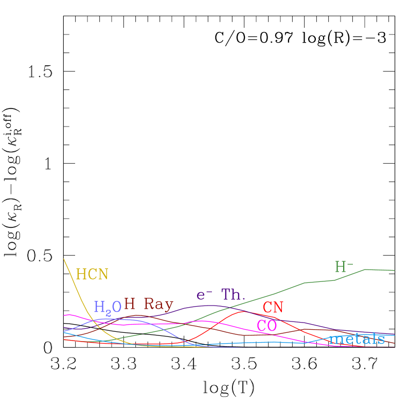
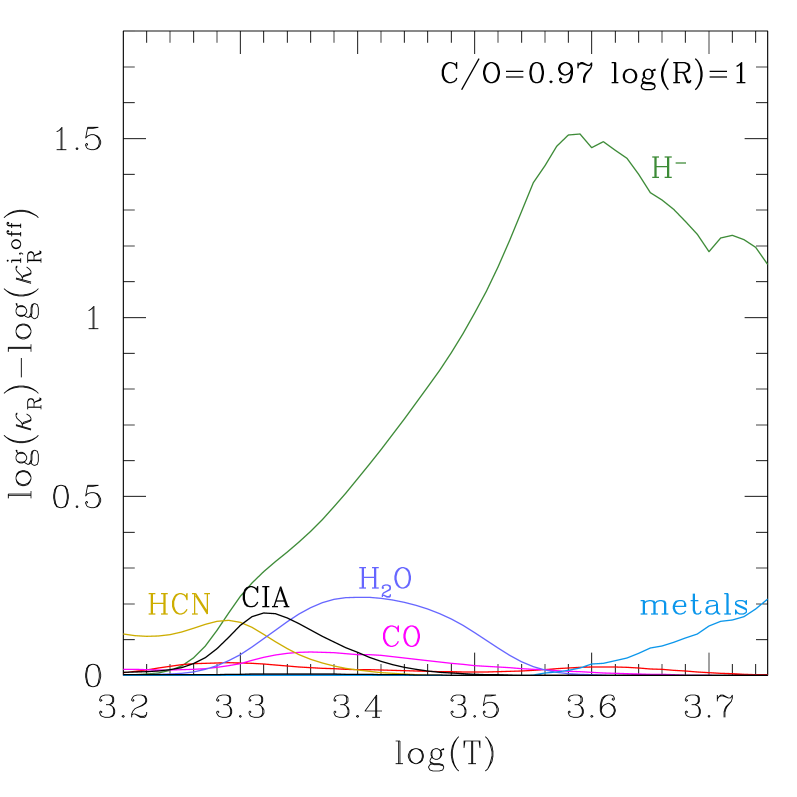
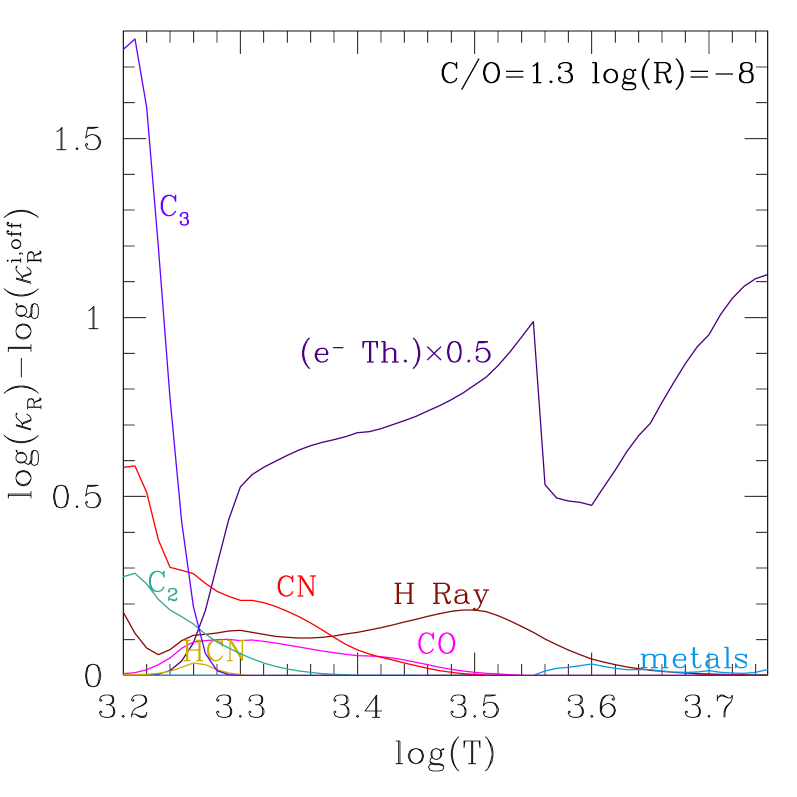
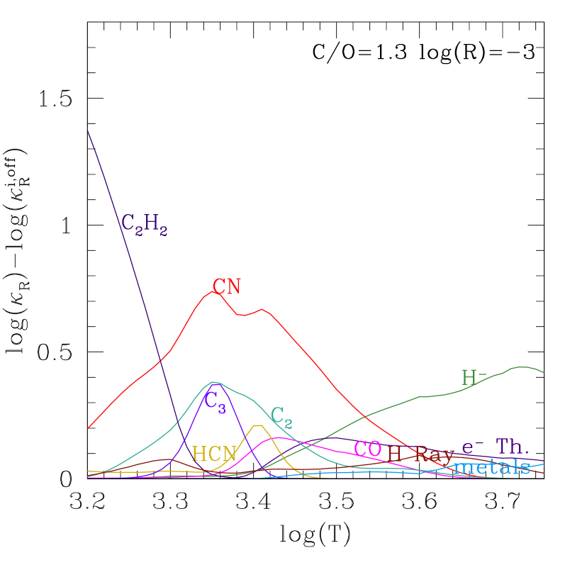
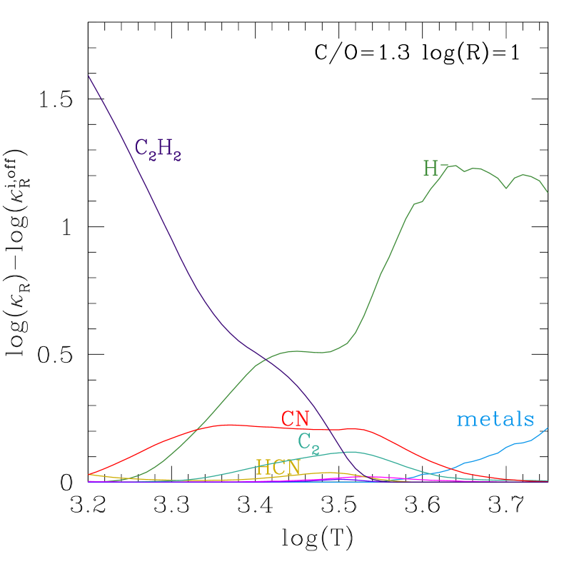
Figure 13: The same as in Fig. 5 but for gas mixtures with C/O=$0.97$ (upper panels) and C/O $=1.3$ (bottom panels), and zoomed into the molecule-dominated temperature region. Note the various opacity bumps of the C-bearing molecules in the C/O=$1.30$ case, while comparable contributions from both O-rich and C-rich molecules are present in the C/O=$0.97$ case.

4.2.2 Opacity sources at increasing C/O ratio

The extreme sensitiveness of the molecular chemistry – for $\log(T)\la 3.5-3.6$ depending on the density – to the C/O parameter has striking consequences on the low-temperature gas opacities, as shown in Fig. 12, relative to $\log(T)=3.3$ and three values of the $R$ parameter. This figure can be interestingly compared with the bottom panels of Fig. 4, describing the case of an oxygen-rich scaled-solar chemistry. For instance, we see that at $\log(T)=3.3$ and $\log(R)=-3$ (bottom-mid panel of Fig. 12) the total monochromatic coefficient $\kappa(\nu)$ for C/O $=1.3$ is mostly determined by the absorption bands of molecules such as HCN and CN, while in a gas with the same thermodynamic conditions and solar C/O $\simeq 0.5$, the dominating species are H₂O, TiO, and VO (see bottom-mid panel of Fig. 4).

At the same temperature and density, and for C/O $=0.97$ (upper-mid panel of Fig. 12) the total coefficient $\kappa(\nu)$ is, on average, lower than in the other two cases, being mostly affected by the absorption bands of CO, while the gaps in between are populated by the weaker molecular bands of H₂O, SiO, ZrO, TiO, etc. At lower densities ($\log(R)=-8$; upper-left panel of Fig. 12) Rayleigh scattering from neutral H and Thomson scattering from free electrons fill the spectral intervals between the CO absorption bands, while at higher densities ($\log(R)=1$; upper-right panel of Fig. 12) the total monochromatic coefficient is completely dominated by molecular absorption, with a sizable contribution by CIA($\textup{H}_{2}/\textup{H}_{2}$) at $\lambda\simeq 2$ $\mu$m, just in correspondence of the maximum $\lambda_{\rm max}$ of the weighting function of the Rosseland mean (see Eq. 28).

The sharp changes in the chemistry and monochromatic coefficient $\kappa(\nu)$ as a function of C/O impact as much strongly on the integrated RM opacity $\kappa_{\rm R}$, which is evident in Figs. 13 – 16.

For the same two C/O values considered above, Fig. 13 shows the contributions of different opacity sources to the RM opacity as a function of the temperature (and assuming $\log(R)=-8,\,-3,\,1$). An instructive comparison with the results for a scaled-solar chemistry can be done with the help of Fig. 5. In the case with C/O $=0.97$ (upper panels of Fig. 13) Rayleigh scattering from hydrogen and Thomson scattering from free electrons dominate for $\log(R)=-8$, becoming comparable with the molecular sources for $\log(R)=-3$. Moreover, we notice that at this C/O value, representing the transition between different chemistry regimes, the opacity pattern is quite heterogeneous as it includes the contributions from both O-bearing and C-bearing molecules. For instance, we see that H₂O is important at lower temperatures, CN shows up at larger temperatures, while CO contributes over a larger temperature interval.

In the case with C/O $=1.3$ (bottom panels of Fig. 13) the most noticeable features at different densities are the following. At $\log(R)=-8$ and $\log(T)\la 3.3$ the largest contribution come from C₃ (and CN, C₂), while at larger temperatures the electron scattering dominates. At $\log(R)=-3$ the high and broad opacity bump of CN that dominates the RM opacity over a wide temperature interval, $3.30\la\log(T)\la 3.55$, while the C₂H₂ contribution is prominent for $\log(T)\la 3.30$. In addition, other C-bearing molecules (C₂, C₃, HCN, CO) provide non-negligible contributions to the RM opacity. Finally, at $\log(R)=1$ the polyatomic molecule C₂H₂ is the most efficient contributor to $\kappa_{\rm R}$ for $\log(T)\leq 3.4$, while the hydrogen anion becomes prominent at higher temperatures.

The complex behaviour of the RM opacities as a function of the C/O ratio is exemplified with the aid of Fig. 14 for $3.2\la\log(T)\la 3.6$, the temperature range in which molecules become the most efficient radiation absorbers. It turns out that while the C/O ratio increases from $0.1$ to $0.9$ the opacity bump peaking at ($\log(T)\simeq 3.3$ for $\log(R)=3$) – mostly due to H₂O – becomes more and more depressed because of the smaller availability of O atoms. Then, passing from C/O $=0.9$ down to C/O $=0.95$ the H₂O feature actually disappears and $\kappa_{\rm R}$ drastically drops by more than two orders of magnitude. In fact, at this C/O value the chemistry enters the transition region already discussed (see Fig. 11), so that most of both O and C atoms are trapped in the CO molecule at the expense of the other molecular species, belonging to both the O- and C-bearing groups. At C/O $=1$ the RM opacity increases at the lowest temperatures, $\log(T)\la 3.3$ , while a sudden upturn is expected as soon as C/O slightly exceeds unity, as displayed by the curve for C/O $=1.05$ in Fig. 14. This fact reflects the drastic change in the molecular equilibria from the O- to the C-dominated regime. Then, at increasing C/O ($1.1$, $1.2$, $1.5$, and $2.0$) the opacity curves move upward following a more gradual trend, which is related with the strengthening of the C-bearing molecular absorption bands.

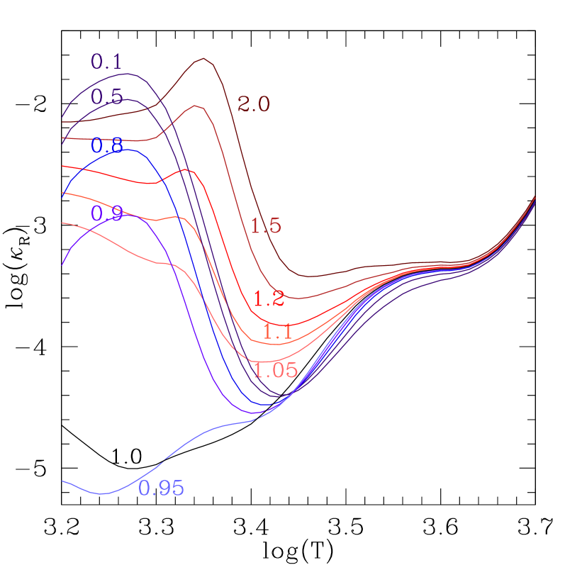
Figure 14: Rosseland mean opacity as a function of temperature, assuming $\log(R)=-3$, and at increasing C/O, from $0.1$ up to $2.0$. The reference composition is defined by ($Z_{\rm ref}=0.02$, $X=0.7$) and assuming the metal abundances scaled-solar to the GAS07 mixture. The abundance of carbon is made vary (hence the actual $Z$), while keeping unchanged that of oxygen.

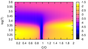
Figure 15: Rosseland mean opacity as a function of the temperature and increasing C/O. adopting the GAS07 solar mixture, and assuming $Z_{\rm ref}=0.02$, $X=0.7$, and $\log(R)=-3$. The abundance of carbon is made vary accordingly to the current C/O ratio (so that the actual metallicity varies as well), while that of oxygen is kept fixed at its scaled-solar value.

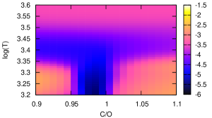
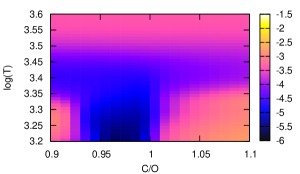
Figure 16: The same as in Fig. 15, but zoomed into a narrower interval around C/O $=1$. The reference solar compositions are AG89 (top panel) and GAS07 (bottom panel).

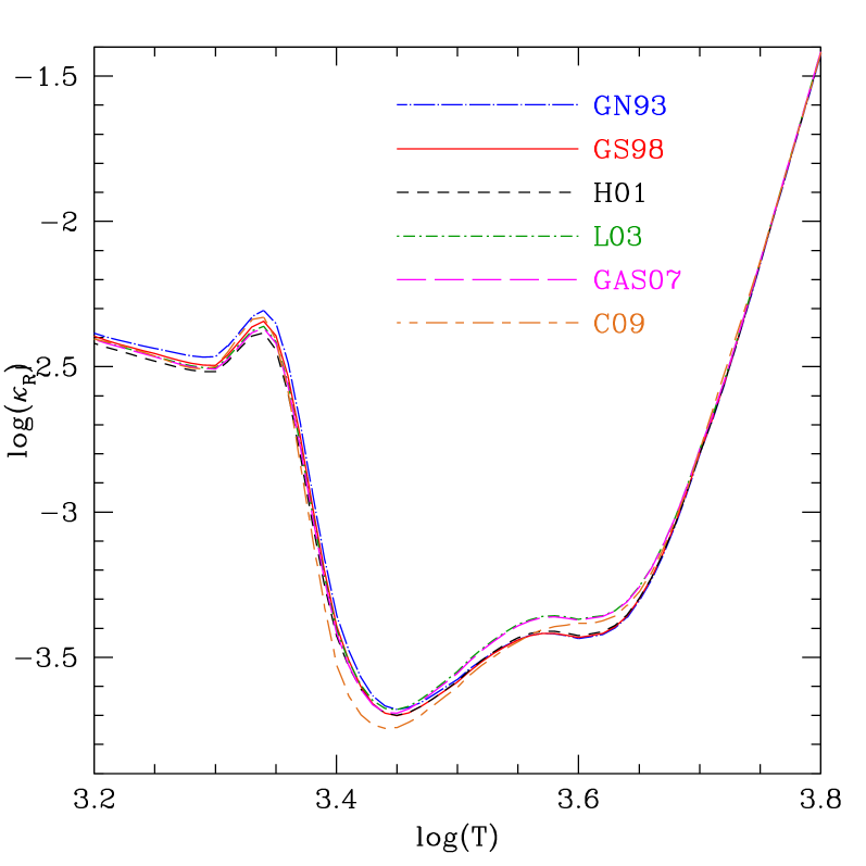
Figure 17: Rosseland mean opacity as a function of the temperature in a gas with $Z_{\rm ref}=0.02$, $X=0.7$, and $\log R=-3$. The adopted chemical composition is characterised by C/O $=1.3$, for various compilations of the reference solar mixture, namely: GN93, GS98, H01, L03, GAS07,and C09. In each case the actual metallicity $Z>Z_{\rm ref}$ because of the increase in C abundance.

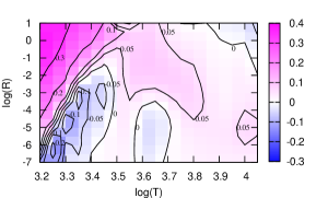
Figure 18: Comparison between our RM opacities and the data from Lederer & Aringer (2009), in terms of $\log(\kappa_{\rm R}^{\rm author})-\log(\kappa_{\rm R}^{\rm\AE SOPUS})$. A few Contour lines are plotted with the corresponding values (in dex). The chemical mixture is defined by $Z_{\rm ref}=0.02$, $X=0.7$, and C/O $\simeq 1.49$. The reference solar composition is L03.

Figure 19: Relation between the total metallicity $Z=f_{Z}\,Z_{\rm ref}$, the C/O ratio and the degree of $\alpha$-enhancement $[\alpha/{\rm Fe}]$, for the three chemical mixtures $A$, $B$, and $C$ defined in Sect. 4.3, and adopting $Z_{\rm ref}=0.02$. The reference solar mixture is GS98.

An enlightening picture of the dependence of the RM opacity on the C/O ratio is provided by Fig. 15, which displays the map of $\log(\kappa_{\rm R})$ at varying temperature and C/O, for fixed $\log(R)=-3$. In this diagram the drop in opacity marking the transition region between the O-rich and C-dominated opacity is neatly visible as a narrow vertical strip of width $0.95\la{\rm C/O}\la 1.00$ (assuming GS98 as reference solar mixture) for temperatures $3.2\leq\log(T)\la 3.35$. This C/O range exactly coincides with the transition interval, (C/O)${}_{\rm crit,1}\la$ C/O $\la$ (C/O)_crit,2, between the O- and C-dominated chemistry. As already mentioned, the lower limit C/O_crit,1 is particularly sensitive to the abundance of silicon relative to oxygen. In respect to this, Fig. 16 shows an enlargement of the opacity map over a narrow interval around C/O $=1$, for two choices of the reference solar composition, i.e. AG89 and GAS07. It is evident that the opacity dip affects a larger C/O range in the case of GAS07 as it corresponds to a higher ratio, (Si/O)${}_{\odot}=7.079\,10^{-2}$, compared to AG89 with (Si/O)${}_{\odot}=4.168\,10^{-2}$. Once chosen the reference solar mixture, one should take this feature into account when computing RM opacity tables at varying C/O ratio, in order to have a good sampling of the critical region, and avoid inaccurate interpolations between grid points belonging to different regimes.

Going back to Fig. 15 we also notice that in the $3.4<\log(T)\la 3.6$ the RM opacity increases with C/O. This fact is due to the increasing contribution from the CN molecule, which is one of the relevant opacity sources in this temperature interval (see bottom-middle panel of Fig. 5 for C/O $=0.54$, and Fig. 13 for C/O $=0.95$ and C/O $=1.3$). It is worth remarking that the effect on the H^- opacity due to the increased carbon abundance is quite modest and only affects the opacity for $\log(T)>3.6$, when ionised carbon is expected to provide some fraction of the available free electrons (see Fig. 22). A more exhaustive consideration of this point is given in Sect. 4.3, when discussing the case of $\alpha$-enhanced mixtures. For larger temperatures the differences in opacity at increasing C/O progressively reduce and practically vanish for $\log(T)>3.7$, when the opacity is controlled by the hydrogen bound-free and free-free transitions.

Let us now briefly comment the sensitiveness of the results to the reference solar mixture. To this aim Fig. 17 illustrates the trend of RM opacity as a function of the temperature in a carbon-rich gas (C/O $=1.3$) with the same $Z_{\rm ref}=0.02$, but different choices of the solar composition. The differences show up for $\log(T)\la 3.65$ and in most cases are modest, thus confirming the key rôle of the C/O ratio in determining the basic features of the molecular opacities. Another point which deserves some attention is the behaviour of the RM opacity in the $3.55\la\log(T)\la 3.65$ interval, which is affected mainly by the CN molecular bands and the negative hydrogen ion H^-. A detailed discussion of this point has been already developed in Sect. 4.1.

4.2.3 Practical hints on interpolation

At given metallicity $Z$ and partitions of the metal species $X_{i}/Z$, interpolation between pre-computed opacity tables is usually performed as a function of the state variables (e.g. $T$ and $R$) and the hydrogen abundance $X$.

When dealing with chemical mixtures with changing elemental abundances, as in the case of the atmospheres of TP-AGB stars, one has to introduce additional independent parameters, in principle as many as the varying chemical species.

Let us consider here the most interesting application, that is the case of TP-AGB stars which experience significant changes in the surface abundances of CNO elements, hence in the C/O ratio. Suppose, for simplicity, to have a chemical mixture with C/O$>1$. Correct interpolation requires that not only the carbon abundance $X_{\rm C}$ is adopted as independent parameter, but also the C/O ratio given its crucial rôle in the molecular chemistry and opacity (see Figs. 11 and 14). In addition, one should pay attention to the drastic changes in $\kappa_{\rm R}$ in the proximity of C/O$=1$. The narrow opacity dip, delimited by the boundaries C/O${}_{\rm crit,1}=1-\varepsilon_{\rm Si}/\varepsilon_{\rm O}$ and C/O${}_{\rm crit,2}=1$ (see Figs. 15-16), should be sampled with at least $1$ or $2$ opacity tables, to avoid substantial mistakes in the interpolated values.

A useful example of an interpolation scheme suitable to treat the complex chemical evolution predicted at the surface of TP-AGB stars undergoing both the third dredge-up and hot-bottom burning can be found in Ventura & Marigo (2009), where the grid of pre-computed opacity tables covers wide ranges of C-N-O abundances (and C/O ratio). Following the formalism introduced in Sect. 3, the adopted independent parameters (besides $T$, $R$ and $X$) are the variation factors $f_{\rm C}$, $f_{\rm C/O}$, and $f_{\rm N}$ (defined by Eq. 31), which are assigned values both $>1$ (i.e. enhancement) and $<1$ (i.e. depletion) to account for the composite effect on the surface composition produced by the third dredge-up and hot-bottom burning. In fact, the C/O ratio may initially increase due to the the third dredge-up and then decrease when hot-bottom burning consumes carbon in favour of nitrogen.

Finally it should be remarked that, when dealing with C-rich mixtures, adopting both $f_{\rm C}$ and $f_{\rm C/O}$ (rather than either $f_{\rm C}$ or $f_{\rm C/O}$) as independent parameters allows more robust results, since the interpolation is piloted by both the actual carbon abundance (mainly affecting the strength of the opacity curves) and the actual C/O ratio (mainly influencing the morphology of the opacity curves; see Fig. 14).

4.2.4 Comparison with other authors

Finally, we close our discussion on the RM opacities for C-rich mixtures by comparing our results with the data calculated by Lederer & Aringer (2009). Figure 18 shows an example for a gas mixture characterised by $Z_{\rm ref}=0.02$, $X=0.7$, and C/O $=1.49$. In general, the agreement between the two calculations is reasonably good, but worse than that for scaled-solar mixtures (see Fig. 7, panel b). The largest differences show up at the lower temperatures, where the RM opacity is dominated by the CN, C₂H₂, C₂, HCN, C₃ molecular bands. This migth appear a bit odd since both sets of calculations adopt basically the same molecular data (see Table 2).

In the range $3.2\la\log(T)\la 3.4$, compared to Lederer & Aringer (2009), ÆSOPUS predicts larger RM opacities (up to $0.1/0.2$ dex) across a strip with $-7\la\log(R)\la 3$, and lower values (up to $\simeq 0.3$ dex) for $\log(R)>-3$.

One likely motivation of the former difference is that the scaling introduced by LA09 to the original $gf$ values in the C₂ line list (Querci et al. 1974) is not included in our calculations. As discussed by LA09 (see their figure 10) not applying this correction to the line strengths of C₂ causes an increase of $\log(\kappa_{\rm R})$ up to $\simeq 0.1$ dex, which is just what we get in terms of $\log(\kappa_{\rm R}^{\rm LA09})-\log(\kappa_{\rm R}^{\rm\AE SOPUS})$ in that particular region of the diagram. On the other hand, more recently Aringer et al. (2009) have shown that omitting this scaling modification to the original C₂ line list improves the comparison between synthetic and observed colours of carbon stars (see their figure 15).

The latter discrepancy between LA09 and ÆSOPUS at larger densities has not a clear reason at present. We note that in this region of the $\log(T)-\log(R)$ diagram, the dominant contribution to the RM opacity is provided by C₂H₂ (see bottom panels of Fig. 12). We are currently investigating possible differences among the partition function and/or dissociation energy of this molecule, adopted in the EOS calculations by LA09 and ÆSOPUS.

4.3 $\alpha$-enhanced mixtures

We will analyse a few important aspects related to RM opacities of $\alpha$-enhanced mixtures, i.e. characterised by having $[\alpha/{\rm Fe}]>0$, according to the notation (in dex):

$$[\alpha/{\rm Fe}]=\log\left(\frac{X_{\alpha}}{X_{\rm Fe}}\right)-\log\left(\frac{X_{\alpha,\odot}}{X_{\rm Fe,\odot}}\right)$$ (36)

where $X_{\alpha,\odot}$ and $X_{\rm Fe,\odot}$ are the total mass fractions of the $\alpha$-elements and Fe-group elements, respectively. In the following we allocate O, Ne, Mg, Si, S, Ca, and Ti in the $\alpha$-group, while V, Cr, Mn, Fe, Co, Ni, Cu, and Zn are assigned to the Fe-group. It should be noticed that, since Fe is by far the most abundant element of its group, the ratio $[\alpha/{\rm Fe}]$ calculated with Eq. (36) coincides with the ratio computed using the abundances in number fraction:

$$[\alpha/{\rm Fe}]=\log\left(\frac{\varepsilon_{\alpha}}{\varepsilon_{\rm Fe}}\right)-\log\left(\frac{\varepsilon_{\alpha,\odot}}{\varepsilon_{\rm Fe,\odot}}\right)$$ (37)

For simplicity in our discussion we take as selected elements all $\alpha$-elements which are given the same $[\alpha/{\rm Fe}]>0$. However, it should be remarked that any other prescription, concerning both the selected elements and the corresponding $[X_{i}/{\rm Fe}]$ (i.e. positive or negative), can be set by the user via the ÆSOPUS interactive web page.

First of all, we call attention to the fact that a given value of the ratio $[\alpha/{\rm Fe}]$ is not sufficient to specify the chemical mixture unambiguously. The same degree of $\alpha$-enhancement may correspond to quite different situations, as exemplified in the following.

Adopting the formalism introduced in Sect. 3 and introducing the quantity $f_{Z}=Z/Z_{\rm ref}$ ($g_{Z}=\varepsilon_{Z}/\varepsilon_{Z_{\rm ref}}$), we define three different $\alpha$-enhanced compositions that, in our opinion, may describe possibly frequent applications. They are characterised as follows (considering the metal abundances expressed in mass fractions):

• Mixture $A$: $Z=Z_{\rm ref}$ hence $f_{Z}=1$; $f_{i}>0$ for $\alpha$-elements (enhanced group); $f_{i}<0$ for any other element (depressed group). In this case the fixed group (with $f_{i}=0$) is empty.

• Mixture $B$: $Z=Z_{\rm ref}$ hence $f_{Z}=1$; $f_{i}>0$ for $\alpha$-elements (enhanced group); $f_{i}<0$ for the Fe-group elements (depressed group); $f_{i}=0$ for any other element (fixed group).

• Mixture $C$: $Z>Z_{\rm ref}$ hence $f_{Z}>1$; $f_{i}>0$ for $\alpha$-elements (enhanced group); $f_{i}<0$ for any other element (depressed group). In this case the fixed group (with $f_{i}=0$) is empty, as for mixture $A$.

For each of the three mixtures considered here, Table 4 lists the variation factors, $f_{i}$ and $g_{i}$, of the most relevant elements, i.e. C, N, O, Fe-group elements, and the metallicity parameter, $f_{Z}$ and $g_{Z}$, as a function of a few selected $[\alpha/{\rm Fe}]$ values. The general analytical derivation of the abundance variation factors as a function of the selected $[X_{i}/{\rm Fe}]$ for the three kinds of mixtures is detailed in Appendix C. Figure 19 displays the expected trends of C/O and $f_{Z}$ at increasing $[\alpha/{\rm Fe}]$ assuming $Z_{\rm ref}=0.02$ and the GS98 solar composition.

For a given $[\alpha/{\rm Fe}]$ value, the three mixtures have distinctive abundance features when compared to the reference composition, i.e. with $Z=Z_{\rm ref}$ and scaled-solar partitions of metals. In particular, for their relevance to the resulting RM opacity, it is worth considering the changes in the CNO abundances, and mostly in the C/O ratio.

$[\alpha/{\rm Fe}]$	Mixture	$f_{\rm C}$	$g_{\rm C}$	$f_{\rm N}$	$g_{\rm N}$	$f_{\rm O}$	$g_{\rm O}$	$f_{\rm Fe-group}$	$g_{\rm Fe-group}$	$f_{Z}$	$g_{Z}$
0.2	$A$	0.714	0.721	0.714	0.721	1.131	1.143	0.714	0.721	1.000	0.990
	$B$	1.000	0.982	1.000	0.982	1.041	1.022	0.657	0.645	1.000	1.018
	$C$	0.714	0.721	0.714	0.721	1.131	1.143	0.714	0.721	1.392	1.387
0.4	$A$	0.491	0.500	0.491	0.500	1.233	1.256	0.491	0.500	1.000	0.982
	$B$	1.000	0.970	1.000	0.970	1.060	1.037	0.426	0.413	1.000	1.031
	$C$	0.491	0.500	0.491	0.500	1.233	1.256	0.491	0.500	2.004	2.000
0.6	$A$	0.329	0.336	0.329	0.336	1.308	1.339	0.329	0.336	1.000	0.977
	$B$	1.000	0.962	1.000	0.962	1.087	1.046	0.273	0.263	1.000	1.039
	$C$	0.329	0.336	0.329	0.336	1.308	1.339	0.329	0.336	2.950	2.972
0.8	$A$	0.215	0.222	0.215	0.222	1.360	1.398	0.215	0.222	1.000	0.973
	$B$	1.000	0.957	1.000	0.967	1.099	1.052	0.174	0.167	1.000	1.045
	$C$	0.215	0.222	0.215	0.222	1.360	1.398	0.215	0.222	4.392	4.513

Table 4: Main characteristics of the $\alpha$-enhanced mixtures described in text. The variation factors of C, N, O, and Fe-group elements, defined by Eqs. (33) for abundances either in mass fraction or in mass fraction, are indicated together with the quantities $f_{Z}=Z/Z_{\rm ref}$ and $g_{Z}=\varepsilon_{Z}/\varepsilon_{Z_{\rm ref}}$. The reference solar composition is GS98.

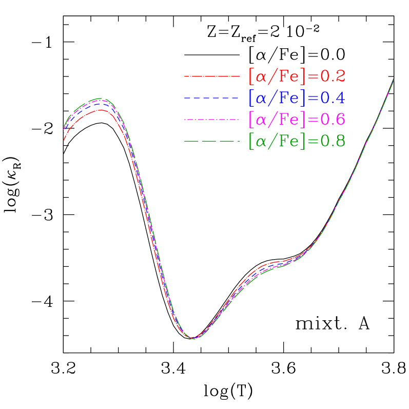
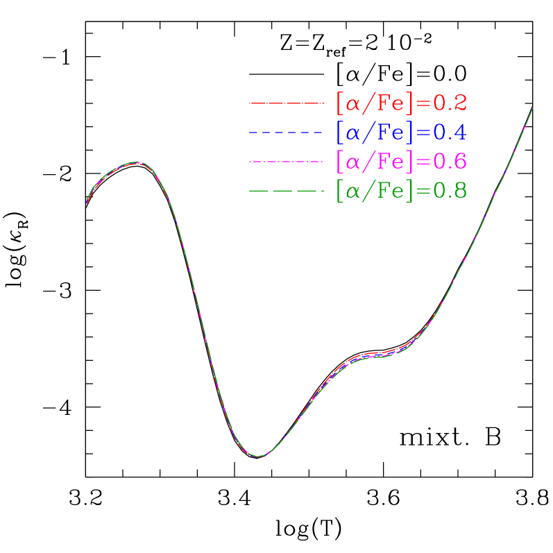
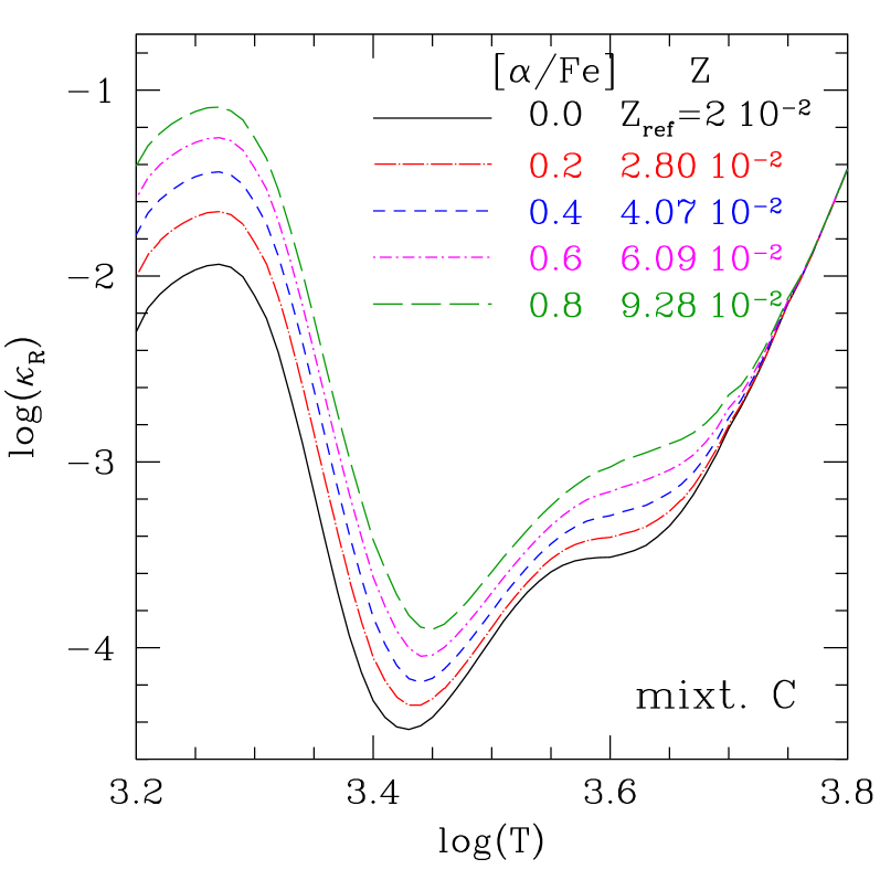
Figure 20: Rosseland mean opacity as a function of temperature and assuming $\log R=-3$, for a gas with ($Z_{\rm ref}=0.02$, $X=0.7$) and various choices of the ratio $[\alpha/{\rm Fe}]$, as indicated. The reference solar mixture is GS98. Results are shown for three choices of the chemical composition, corresponding to mixtures $A$, $B$, $C$ described in the text.

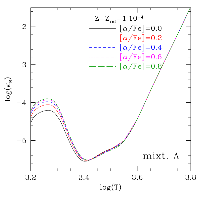
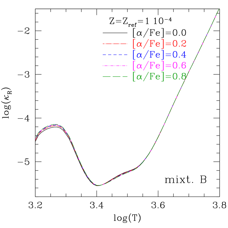
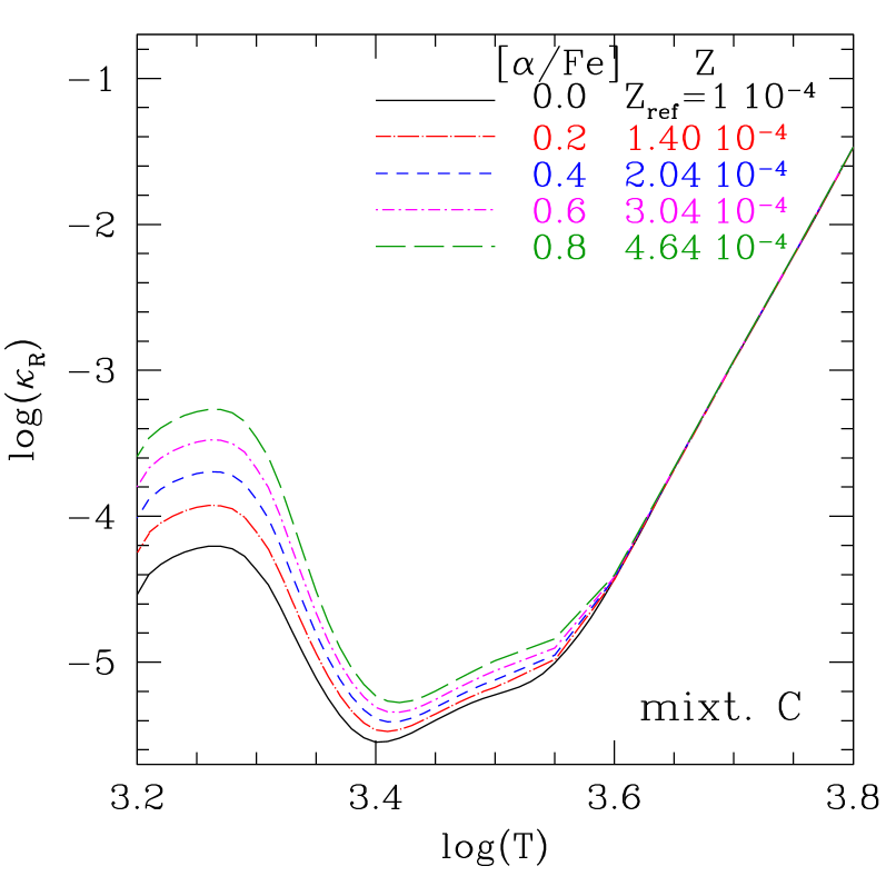
Figure 21: The same as in Fig. 20, but for $Z_{\rm ref}=0.0001$.

• Mixture $A$ is depleted both in the iron-group elements as well as in carbon and nitrogen. For instance, at $[\alpha/{\rm Fe}]=0.4$, the abundances of the Fe-group elements are almost halved and the same applies to C and N, while O is augmented by $\sim 23\%$. As a consequence the C/O ratio decreases significantly, passing from (C/O)${}_{\odot}\sim 0.49$ down to (C/O)${}_{\odot}\sim 0.19$. In general, the ratio C/O lowers considerably at increasing $[\alpha/{\rm Fe}]$.

• Mixture $B$ is depleted in the iron-group elements, while C and N are left unchanged. At $[\alpha/{\rm Fe}]=0.4$, the abundances of the Fe-group elements are depressed by $\sim 43\%$, while O is increased by only $\sim 6\%$. In this case the C/O ratio is just little affected, changing from (C/O)${}_{\odot}\sim 0.49$ to (C/O)${}_{\odot}\sim 0.46$. In general, the ratio C/O slightly decreases at increasing $[\alpha/{\rm Fe}]$.

• Mixture $C$ has the same characteristics of mixture $A$ in terms of metal partitions, i.e. $(X_{i}/Z_{\rm ref})_{A}=(X_{i}/Z)_{C}$, but with a different metallicity. It follows that the $C$ case shares with $A$ the same elemental ratios, so that the C/O declines significantly at increasing $[\alpha/{\rm Fe}]$, while the total metallicity increases. For instance, at $[\alpha/{\rm Fe}]=0.4$ mixture $C$ corresponds to a metallicity $Z\simeq 2\,Z_{\rm ref}$ (see Table 4 and Fig. 19).

The aforementioned differences in the chemistry among the mixtures $A$, $B$, and $C$ affect the resulting RM opacities, as displayed by Fig. 20 for $Z_{\rm ref}=0.02$ and Fig. 21 for $Z=0.0001$, both assuming $X=0.7$ and $\log(R)=-3$. Let us first discuss the results of the $A$ and $B$ cases with $Z_{\rm ref}=0.02$. With respect to mixture $A$ (left panel of Fig. 20), we see that at increasing $\alpha$-enhancement, the opacity variations show up with opposite trends in two temperature intervals, namely: at intermediate temperatures, $3.50\la\log(T)\la 3.65$, and at lower temperatures, $3.2\la\log(T)\la 3.4$. Specifically, the opacity knee at $\log(T)\simeq 3.55$ slightly smooths, while the opacity bump at $\log(T)\simeq 3.3$ becomes more prominent with increasing $[\alpha/{\rm Fe}]$.

As already discussed in Sect. 4.1, in the $3.5\la\log(T)\la 3.6$ interval the most effective opacity source is the negative hydrogen ion (see lower middle panel of Fig. 5), which positively correlates with the electron density, $n_{e}$. Figure 22 shows that in this temperature range the principal electron donors are elements with relatively low-ionisation potentials, mainly Mg, Si, Fe, Al, Ca, and Na, which involve both the enhanced group and the depressed group. For this reason, it turns out that in the $\alpha$-enhanced mixture of type $A$ the decreased number of electrons contributed by Fe (together with C, Na, Al, Cr, Ni) is practically counter-balanced by the increased number of electrons removed from the $\alpha$-atoms such as Mg, Si, and S. The net effect is just a very little reduction in the electron density. In the case exemplified in Fig. 22 even a large $\alpha$-enhancement $[\alpha/{\rm Fe}]=0.6$ corresponds to a reduction of $n_{e}$ by just $\sim 6\%$ at $\log(T)=3.55$. In turn, this small variation in $n_{e}$ produces a minor reduction of the H^- opacity. From a careful inspections of the results we find that the depression of the opacity knee at $\log(T)\simeq 3.55$ should be rather ascribed to the weakening of the CN molecular absorption bands, which reflects the depression of both carbon and nitrogen abundances in mixture $A$. In fact, at these temperatures and $\log(R=-3)$ the CN contribution to the RM opacity is not negligible (see lower middle panel of Fig. 5).

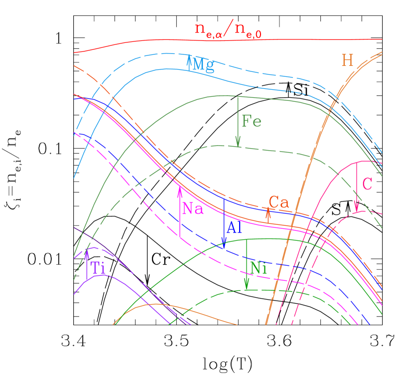
Figure 22: Contributions of free electrons $\zeta_{i}=n_{e,i}/n_{e}$, normalised to the total electron density $n_{e}$, provided by different ions as a function of temperature, in two gas mixtures with ($Z=Z_{\rm ref}=0.02$, $X=0.7$, $\log(R)=-3$) and different partitions of the $\alpha$-elements, namely: $[\alpha/{\rm Fe}]=0.0$ (scaled-solar abundances; solid lines), and $[\alpha/{\rm Fe}]=+0.6$ ($\alpha$-enhanced mixture of type $A$; dashed lines). The arrows indicate the increasing/decreasing trends when passing from $[\alpha/{\rm Fe}]=0.0$ to $[\alpha/{\rm Fe}]=+0.6$. The highest curve (in red) displays the ratio $n_{e,\alpha}/n_{e,0}$, i.e. the electron density of the $\alpha$-enhanced composition relative to the scaled-solar case. The reference solar mixture is GS98.

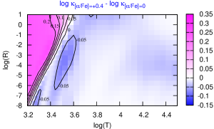
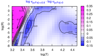
Figure 23: Differences in RM opacities between $\alpha$-enhanced mixtures, with $[\alpha/{\rm Fe}]=+0.4$ (top panel) and $[\alpha/{\rm Fe}]=+0.8$ (bottom panel), and a scaled-solar composition according to GS98. The $\alpha$-enhanced mixtures are constructed according to the $A$ scheme. In all case we assume ($Z_{\rm ref}=0.02$, $X=0.7$). Contour lines, with an incremental step of $0.05$ dex, are over-plotted to guide the comparison.

With respect to mixture $B$, we note that in the same temperature range, i.e. $3.50\la\log(T)\la 3.65$, the variations of the RM opacity at increasing $[\alpha/{\rm Fe}]$ are smaller than for mixture $A$, almost negligible. In fact, in mixture $B$ the carbon and nitrogen abundances are left unchanged so that the opacity contribution from CN is not expected to vary as well. Furthermore, the same arguments on the electron density, discussed for mixture $A$, hold also in this case, and the H^- opacity contribution is predicted to change just slightly.

Let us now consider the temperature interval $3.2\la\log(T)\la 3.4$, which is characterised by the opacity bump due to the molecular absorption bands of H₂O, TiO, and ZrO. We see from Figure 19 (bottom panel) that the opacity peak grows at increasing $[\alpha/{\rm Fe}]$, reflecting the decrease of the C/O ratio. In fact, the concomitant enhancement of oxygen and the depression of carbon favour the chemistry of the O-bearing molecules, thus strengthening the opacity contributions of H₂O, TiO, and ZrO at those temperature. The reader should refer to Sect. 4.2 for a broad analysis of the dependence of the low-temperature opacity on the C/O ratio. For the same reasons, in the case of mixture $B$ the opacity bump is practically insensitive to changes in $[\alpha/{\rm Fe}]$, since the decrease of C/O ratio is just marginal, as shown in Fig. 19.

Figure 23 shows the differences in terms of $\Delta\log(\kappa_{\rm R})$ expected when the chemical composition of the gas is enhanced in $\alpha$-elements, according to mixture $A$. The same comments already spent for Fig. 20 (left panel) hold here. At increasing $[\alpha/{\rm Fe}]$ negative deviations mostly take place in the region dominated by the absorption of H^-, while positive variations show up at lower temperatures, over a well-defined region in the $\log(T)-\log(R)$ diagram, the boundaries of which are determined by the thermodynamic conditions required to form H₂O efficiently (see top panels of Fig. 5), thus becoming narrower at decreasing $R$.

The case of mixture $C$ deserves different remarks. At increasing $[\alpha/{\rm Fe}]$ the RM opacity is predicted to be larger all over the temperature range $3.2\la\log(T)\la 3.75$, and the variations are always larger than for the other two mixtures. This fact can be explained simply as a metallicity effect, since the global metal content increases with the $[\alpha/{\rm Fe}]$ as indicated by the $f_{Z}$ parameter (see Fig. 19). Therefore, mixture $C$ shares with mixture $A$ the same partition of metals (i.e. the same variation factors $f_{i}$; see Table 4), but their abundances are all higher, including those belonging to the depressed group. The net effect is systematic increase of the RM opacity with $[\alpha/{\rm Fe}]$.

Finally, a cautionary comment is worth being made. It should be noticed that the while the $\alpha$-elements are the same for the three mixtures here considered, the differences deal with i) which elements are assigned to the depressed group and to the fixed group, and ii) the total metallicity. The results discussed above show clearly that this an important point which impacts on the resulting RM opacities. Therefore, when using RM opacity tables one should be always aware of how the underlying $\alpha$-enhanced mixture has been constructed, since his/her results may be importantly affected. This aspect has been recently discussed by Dotter et al. (2007). To our knowledge available RM opacity tables adopt $\alpha$-enhanced mixtures similar to our $A$ scheme (e.g. Ferguson et al. 2005 and related website of the Wichita State University group).

4.4 Other peculiar mixtures: C-N-O-Na-Mg-Al abundance anti-correlations

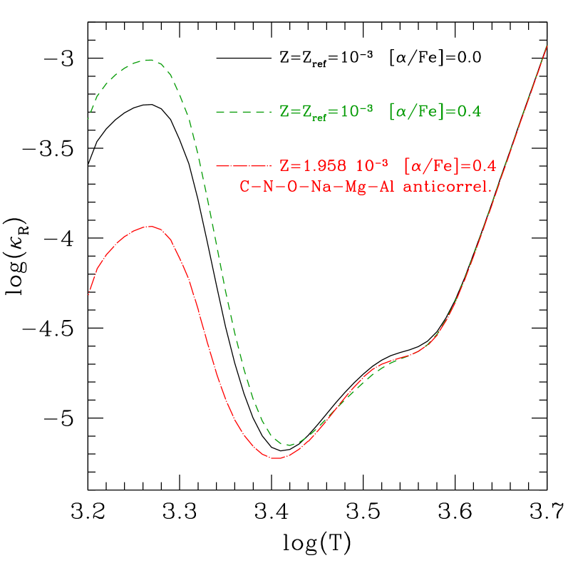
Figure 24: Rosseland mean opacity as a function of temperature and assuming $\log R=-3$, for a gas with ($Z_{\rm ref}=0.001$, $X=0.7$). The reference solar mixture is GS98. Results are shown for three chemical mixtures, namely: i) scaled-solar abundances of metals; enhanced abundances of $\alpha$-elements with $[\alpha/{\rm Fe}]=+0.4$ (according to mixture $A$; see Sect. 4.3); peculiar chemical pattern characterised by additional C-N-O-Na-Mg-Al abundance variations superimposed to the $\alpha$-enhanced mixture. See the text for details.

Another relevant case is suggested by the peculiar chemical patterns observed in stars of Galactic globular clusters (GGC), being characterised by striking abundance anti-correlations between C-N and O-Na, and Mg-Al, which are in turn superimposed on a typical $\alpha$-enhanced mixture (e.g. Gratton et al. 2001). Stellar evolution models including low-temperature RM opacities suitable for these particular compositions have been recently calculated (Salaris et al. 2006; Pietrinferni et al. 2009).

Figure 24 shows an example of RM opacities computed with ÆSOPUS for a gas mixture which would represent the pattern of extreme C-N-O-Na-Mg-Al anti-correlations, as measured in GGC stars (Carretta et al. 2005). The adopted abundance scheme is the following. We start with our reference scaled-solar mixture, characterised by $Z_{\rm ref}=0.001,\,X=0.7$ and GS98 solar composition. Then we construct a second composition with $[\alpha/{\rm Fe}]=+0.4$ following the prescriptions for mixture $A$ (see Sect. 4.3). The C/O decreases from (C/O)${}_{\odot}\simeq 0.49$ to $\simeq 0.19$, while the total metallicity is preserved. This fact explains the growth of the opacity peak due to H₂O at $\log(T)\la 3.4$ in the $\alpha$-enhanced mixture. The reader should go back to Sect. 4.3 for an extensive discussion on the differences between the two RM opacity curves.

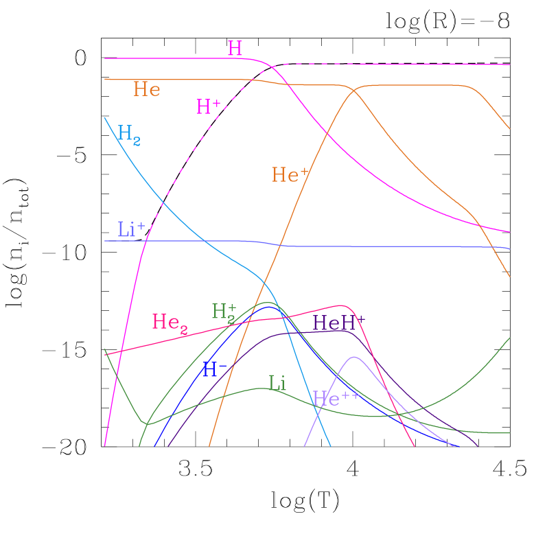
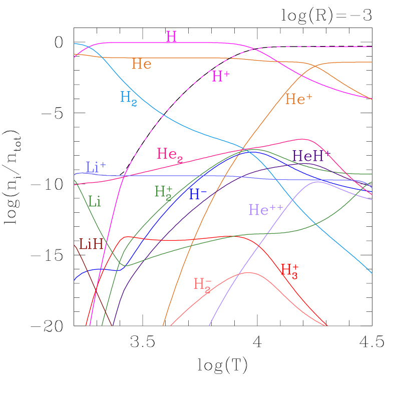
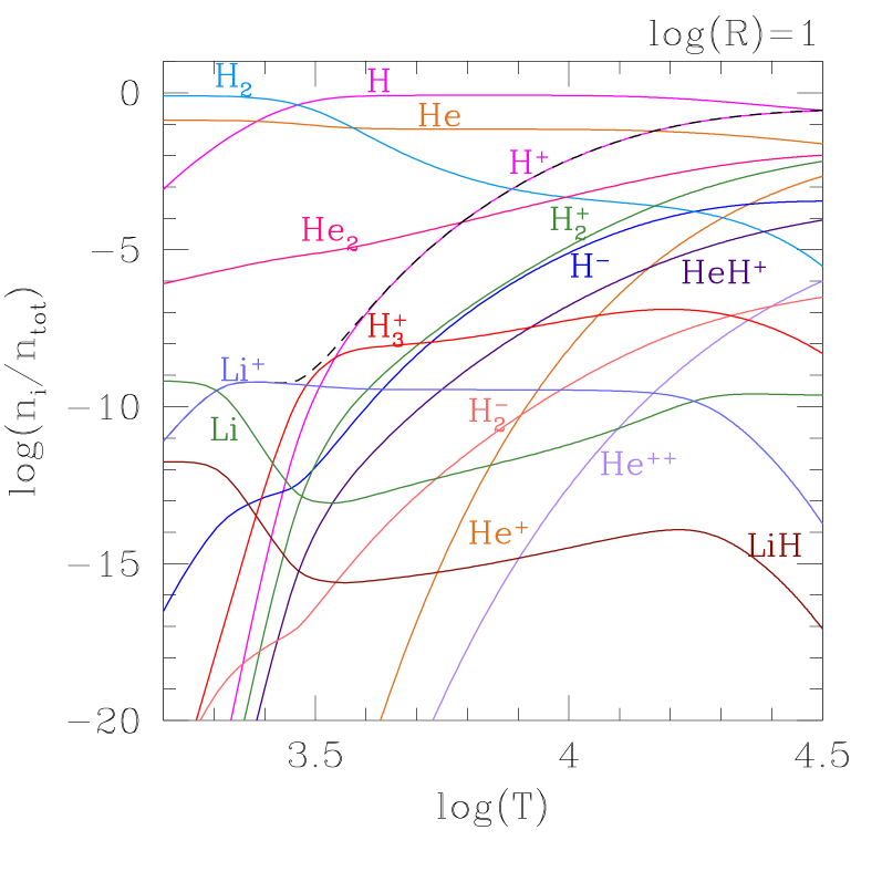
Figure 25: Concentrations of a few atomic and molecular species as a function of the temperature in a gas with primordial composition, adopting $Z_{\rm ref}=0$, $X=0.7521$, and a lithium abundance of $\varepsilon_{\rm Li}/\varepsilon_{\rm H}=4.15\times 10^{-10}$, and assuming $\log(R)=-3$. The fraction of free electrons, $n_{e}$ is depicted by a dashed black line.

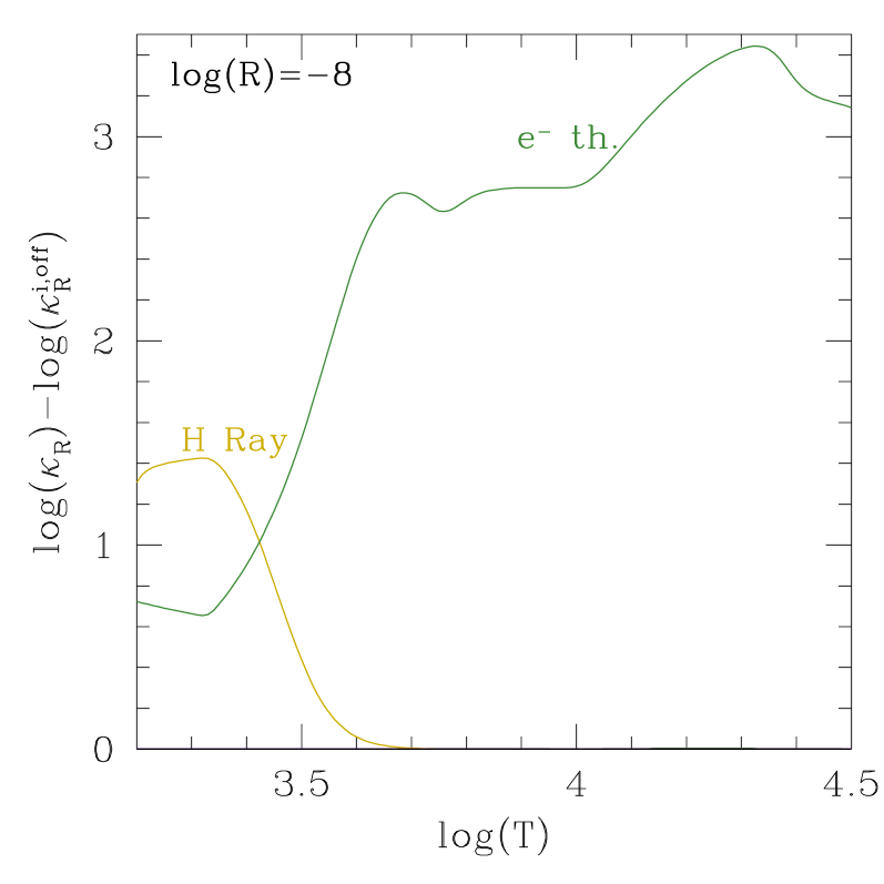
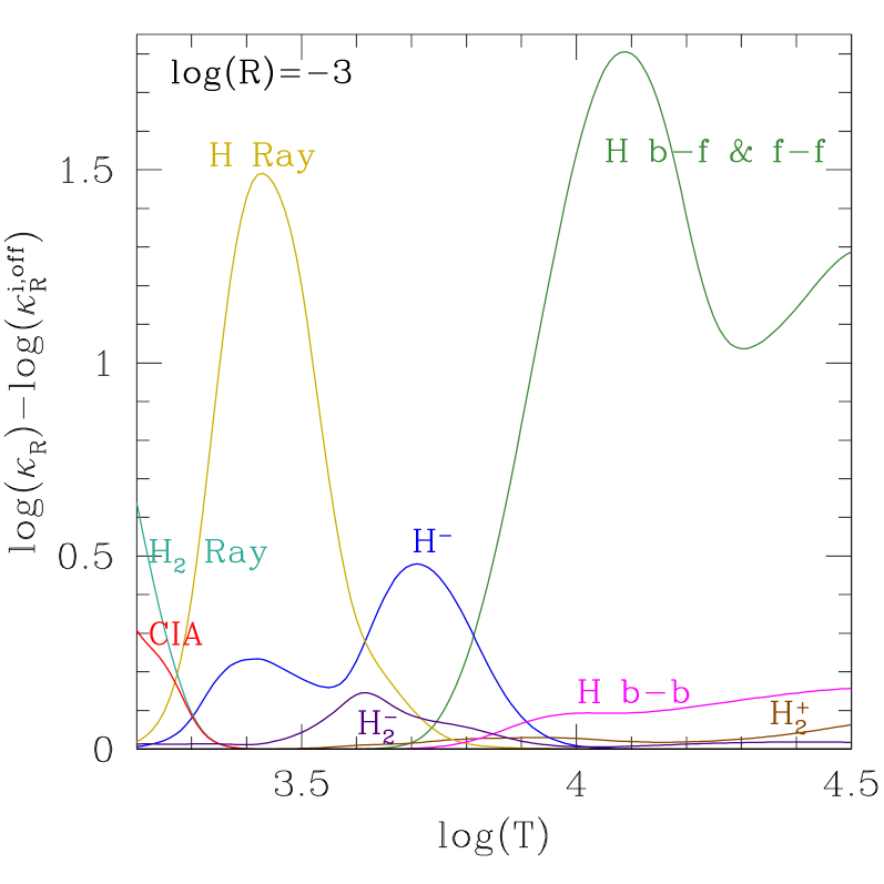
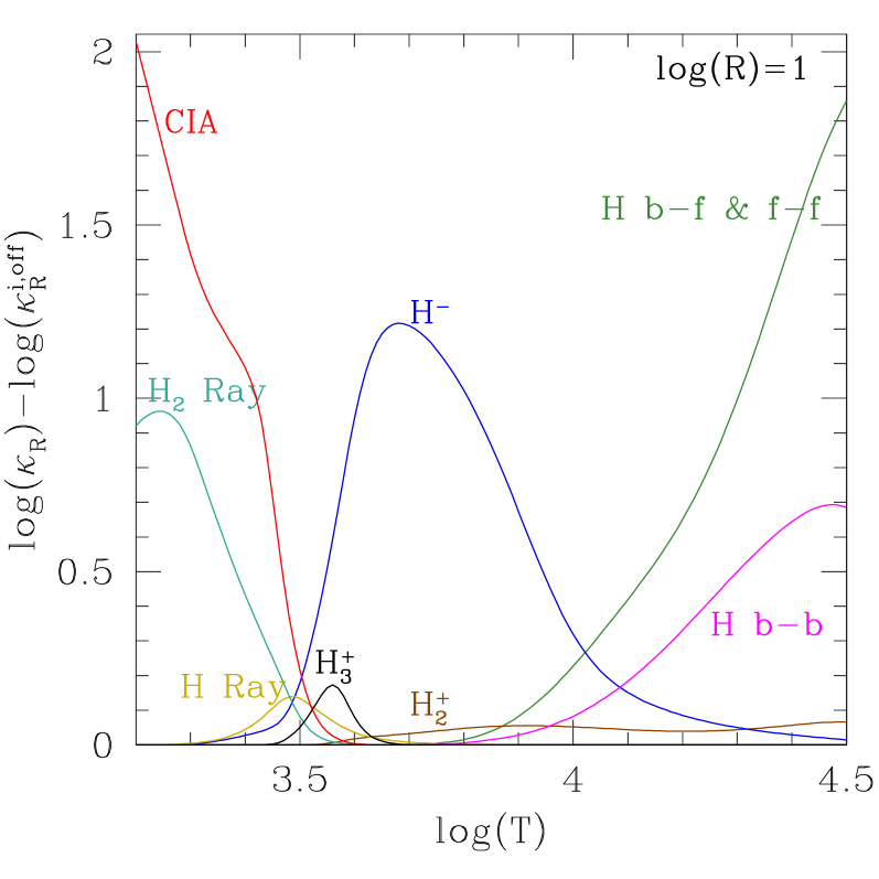
Figure 26: The same as in Fig. 5 but for a primordial composition with $Z_{\rm ref}=0$ and $X=0.7521$ and assuming three of the $R$ parameter, as indicated. Note the prominent bump of the CIA sources, mainly due to H₂-H₂ collisions, at lower temperatures in the case for $\log(R)=1$.

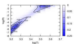
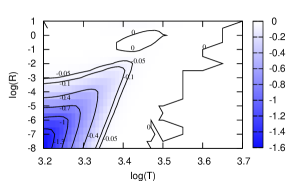
Figure 27: Difference $\Delta\log(\kappa_{R})=\log(\kappa_{\rm R})-\log(\kappa_{\rm R}^{\rm i,off})$ between the full RM opacity of our assumed primordial composition and the reduced opacity obtained either leaving out the chemistry of H${}_{3}^{+}$ (left panel), or assuming a Li-free mixture (right panel). A few contour lines, labelled with the corresponding values (in dex), are superimposed to guide the eye.

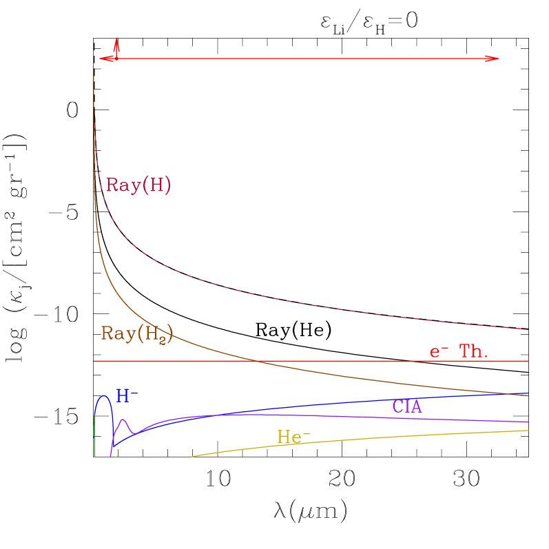
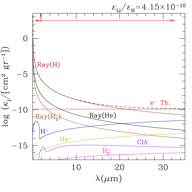
Figure 28: The same as in Fig. 4 but for a primordial composition with $Z_{\rm ref}=0$ and $X=0.7521$, and assuming $\log(R)=-8$ and $\log(T)=3.3$. The arrows bracket the spectral range across which the weighting function of the RM decays by a factor $1/100$. The left panel shows the results for a lithium-free mixture, whereas the right panel illustrates the case for a primordial lithium abundance, as predicted by the SBBN in accordance with WMAP (Coc et al. 2004).

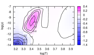
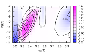
Figure 29: Comparison in terms of $\log(\kappa_{\rm R}^{\rm H04})-\log(\kappa_{\rm R}^{\rm\AE SOPUS})$ between our opacity results and the tabulated values by Harris (2004) for a metal-free mixture with ($Z=0$, $X=0.7$). A few contour lines, labelled with the corresponding values (in dex), are superimposed to help the comparison. Note how much the differences become significant at lower temperatures when assuming $\varepsilon_{\rm Li}/\varepsilon_{\rm H}=4.15\times 10^{-10}$ in our calculations (left panel), while they drastically reduce adopting $\varepsilon_{\rm Li}/\varepsilon_{\rm H}=0$ (right panel).

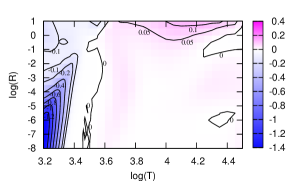
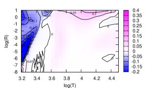
Figure 30: The same as in Fig. 29, but in terms of $\log(\kappa_{\rm R}^{\rm F05})-\log(\kappa_{\rm R}^{\rm\AE SOPUS})$ between our opacity results and the tabulated values by Ferguson et al. (2005) for a metal-free mixture with ($Z=0$, $X=0.7$).

Finally we perturb the second mixture and add the C-N-O-Na-Mg-Al anti-correlation pattern assuming the following abundance variations in dex (see Salaris et al. 2006): $\log(f_{\rm C})=-0.6$; $\log(f_{\rm N})=+1.8$; $\log(f_{\rm O})=-0.8$; $\log(f_{\rm Na})=+0.8$; $\log(f_{\rm Mg})=-0.4$; and $\log(f_{\rm Al})=+1.0$. By doing so the total metallicity almost doubles, $Z=1.97\,10^{-3}$, while the ratio $[{\rm Fe/H}]\simeq-1.5$ remains the same as in the genuine $\alpha$-enhanced mixture.

The increase in metallicity is mainly due to the augmented N abundance, while those of C and O both drop considerably. The resulting C/O ratio is now $\simeq 0.31$, and the total $\varepsilon_{(\rm C)}+\varepsilon_{(\rm{O})}$ is decreased by $\simeq 83\%$. This fact explains that, despite of the overall increase in $Z$, the opacity curve of the peculiar mixture lies systematically lower than the others in the temperature region dominated by the H₂O bump.

In the temperature interval $3.4\la\log(T)\la 3.6$ the differences in RM opacity among the three curves in Fig. 24 are quite small and should be mainly ascribed to differences in the abundances of electron donors, which in turn affect the strength of the H^- opacity.

4.5 Metal-free mixtures

The last important application we discuss here deals with RM opacities suitable for zero-metallicity gas with a primordial composition. Following the standard Big Bang nucleosynthesis (SBBN), the most abundant elements to be synthesised first were H, He, with small quantities of D and Li, and tiny (and negligible) traces of Be and B. In this work we assume a primordial mixture made up of $X=0.7521$, $\varepsilon_{\rm Li}/\varepsilon_{\rm H}=4.15\times 10^{-10}$ (ratio of abundances by number), and $Y=1-X-$Li (hence $Z=0$), these values being predicted by the SSBN in accordance with the baryon-to-photon ratio as derived by the Wilkinson Microwave Anisotropy Probe (WMAP; Coc et al. 2004). The abundances of B ad Be are reasonably neglected, since $\varepsilon_{\rm Be}/\varepsilon_{\rm H}$ and $\varepsilon_{\rm B}/\varepsilon_{\rm H}<10^{-17}$ according to models of primordial nucleosynthesis (Thomas et al. 1993, 1994).

Figure 25 shows the predicted chemistry of a primordial gas as a function of the temperature and three selected values of the $R$ parameter, and correspondingly Fig. 26 illustrates the relative contributions of the most important opacity sources to the total RM opacity. It is worth noticing the following points.

At lower densities (e.g. left panels with $\log(R)=-8$) the abundance of the negative hydrogen ion H^- grows very little, the H₂ molecule does not form efficiently even at the lowest temperatures, and the concentration of H${}_{3}^{+}$ is negligible (reaching a maximum value $\log(n/n_{\rm tot})\sim-20.8$ at $\log(T)\sim 3.35$). The total RM opacity is completely dominated by scattering processes, namely Thomson scattering from free electrons at higher temperatures, and scattering from hydrogen atoms at lower temperatures.

At increasing densities (e.g. going from $\log(R)=-3$ to $\log(R)=1$) the abundances of most relevant species like H₂ , H^-, H${}_{3}^{+}$ grow higher and higher. At intermediate densities (i.e. middle panel of Fig. 26) we may distinguish three different temperature ranges, namely: $3.2\la\log(T)\la 3.6$ dominated by scattering from H atoms, $3.6<\log(T)\la 3.85$ characterised by the contribution of H^-, and $3.85\la\log(T)\la 4.5$ controlled by the continuous absorption of H (bound-free and free-free transitions). Free electrons are provided by H⁺ and Li⁺ as in the previous case.

Finally, at the highest densities (i.e. right panel of Fig. 26) we notice that the RM opacity in the low-temperature region $3.2\la\log(T)\la 3.5$ is determined by collision-induced absorptions (mainly CIA due to H₂-H₂ collisions); the H^- opacity bump is prominent in the range $3.2<\log(T)\la 4.0$; and continuous and discrete processes due to H are dominant at higher temperatures.

It should be remarked that Thomson scattering as well as absorption by negative ions (i.e. H^-, H${}_{2}^{-}$, He^-) crucially depend on the amount of available free electrons. By looking at the curve of the electron concentration (dashed line) in Fig. 25 we see that, among the positive ions, three are the main electron donors in a primordial gas, i.e. H⁺, Li⁺, and H${}_{3}^{+}$. Ionisation of hydrogen atoms accounts for $n_{e}$ at the higher temperatures down to $\log(T)\sim 3.6-3.3$ depending on the density, ionised lithium practically provides all free electrons at lower temperatures, while H${}_{3}^{+}$ contributes free electrons only over an intermediate temperature range depending on the gas density.

Let us first consider the case of H${}_{3}^{+}$. The importance of this ion for the electron budget of a primordial gas has been extensively discussed by Lenzuni et al. (1991) and Harris et al. (2004, hereafter also H04). In this latter paper the authors have pointed out that the inclusion of H${}_{3}^{+}$, with the most recent partition function of Neale & Tennyson (1995), may increase the RM opacity mostly via an indirect effect on the chemistry, i.e. by favouring larger concentrations of H^- and, to a less extent, via the direct absorption by H${}_{3}^{+}$. The authors have also analysed possible effects on the evolution of very low-mass stars of zero-metallicity. In ÆSOPUS we have included the H${}_{3}^{+}$ chemistry, its free-free opacity, while neglecting the H${}_{3}^{+}$ line opacity. However, as shown by H04, this latter provides a small contribution (few $\%$) to the RM opacity in most cases, with a peak of $15\%$ at certain temperatures and densities. Figure 27 (left panel) displays the region in the $\log(T)-\log(R)$ plane which is affected by the H${}_{3}^{+}$ via its inclusion/omission in the gas chemistry. The differences in $\log(\kappa_{\rm R})$ are always negative along a diagonal strip in the $\log(T)-\log(R)$ diagram, meaning that the neglecting H${}_{3}^{+}$ would lead to underestimate the gas opacity because we omit its contribution to $n_{e}$ (hence weakening the H^- opacity and the Thomson electron scattering), as well as its contribution as a true absorber (the free-free continuum in our computations).

The case of Li is perhaps more interesting since the primordial abundance of this element is predicted by the SBBN and accurately constrained by WMAP. An extensive analysis on the importance of Li for the opacity of the primordial gas has been carried out by Mayer & Duschl (2005), to whom the reader should refer for a detailed discussion. Our computations essentially agree with the findings of Mayer & Duschl (2005). From the inspection of the right panel of Fig. 27 one can see that even a low concentration of Li notably impacts on the resulting RM opacity, the effect being more pronounced at lower temperatures and lower densities. For $\log(T)=3.2$ and $\log(R)=-8$ the difference in opacity is sizable, reaching a value as high as $\Delta\log(\kappa_{\rm R})\simeq 1.6$! Figure 28 helps to get a better insight of the rôle of Li: when including it in the primordial chemistry the total monochromatic absorption coefficient rises for $\lambda>15\,\mu$m due to the increased contribution of the Thomson electron scattering. In fact, a larger amount of free electrons is provided by the first ionisation of lithium, as shown in Fig. 25 (left panel).

Finally, in Figs. 29-31 we present a few comparisons with recently published RM opacity data for zero-metallicity gas, namely: Harris et al. (2004), Mayer & Duschl (2005), and Ferguson et al. (2005). In general the agreement is relatively good, mostly comprised within $\pm 0.2$ dex, except for the large differences (up to $-1.2-1.4$ dex) that arise in the comparison with H04 and F05 at lower temperatures and densities. These discrepancies should be likely ascribed to their neglecting of Li in the chemical mixture, since they drastically reduce when we omit Li from the equation of state. We are not able to find clear reasons to the remaining deviations for $\log(T)<3.5$, temperatures at which Rayleigh scattering from H and H₂, Thomson scattering from electrons, and CIA are the dominant opacity contributors at varying density. In general, differences in the thermodynamic data and input physics adopted to describe the processes listed in Table 2.1.4 might provide a reasonable explanation.

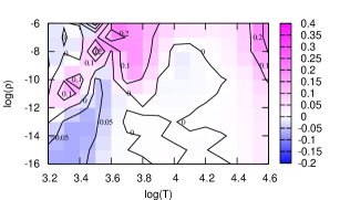
Figure 31: The same as in Fig. 29 in terms of $\log(\kappa_{\rm R}^{\rm M05})-\log(\kappa_{\rm R}^{\rm\AE SOPUS})$ between our opacity results and the tabulated values by Mayer et al. (2005) for a metal-free mixture with $Z=0$, $X=0.7521$, and $\varepsilon_{\rm Li}/\varepsilon_{\rm H}=4.15\times 10^{-10}$.

5 Final remarks

We have developed a new tool, ÆSOPUS, for computing Rosseland mean opacities of an ideal gas in the low-temperature regime, $3.2\leq\log(T)\leq 4.5$. The access to ÆSOPUS is made public via an interactive web-interface (http://stev.oapd.inaf.it/aesopus), which enables the user to specify with large freedom the input parameters, i.e. the grid of the state variables $T$ and $R$, the reference solar composition, the total metallicity, and the abundance enhancement/depletion of all chemical elements, from H to U.

The Rosseland mean gas opacities, produced with a good accuracy (comparable to that of other opacity codes), are delivered in a tabular form within a reasonably short time. At present, the typical computation time for one table at fixed chemical composition, arranged with the default $T-R$ grid, i.e. containing $N_{T}\times N_{R}=67\times 19=1273$ opacity values, is less than $50$ s with a 2.0 GHz processor. Such a fast performance is attained thanks to the optimised use of the opacity sampling method to describe molecular line absorption, and the adoption of pre-tabulated absorption cross-sections for metals (from the Opacity Project database). In this way the line-opacity data is suitably arranged prior to the opacity computations, a process that, if otherwise performed on-the-fly, is in principle more accurate but at the cost of extremely long computing times (e.g. Ferguson et al. 2005).

On the other hand, several tests illustrated in the paper have proved that our procedure, besides being fast, is as well suitable to produce fairly accurate Rosseland mean opacities, to which the very fine spectral details are not critical as they are washed out, by construction, in the harmonic average of the monochromatic coefficient.

First applications of ÆSOPUS opacity tables in stellar evolutionary calculations performed with the Padova code for both scaled-solar (Bertelli et al. 2009), and $\alpha$-enhanced mixtures (Bressan et al., in prep.), and with the ATON code for C-N-O varying mixtures along the AGB (Ventura & Marigo 2009) have yielded promising results. In particular, we find that the differences in the effective temperature of giant (RGB and AGB) models brought about by the adoption of different opacity data for the same chemical composition (e.g. ÆSOPUS, Ferguson et al. 2005, Lederer & Aringer 2009) amount to a few tens of degrees, in most cases lower than (or comparable to) the typical uncertainty of the semi-empirical $T_{\rm eff}$-scale of red giants.

We wish all interested researchers may benefit from an easy access to the low-temperature opacity data. Feedback and suggestions are welcome.

Appendix A EOS under ICE conditions: numerical details

The ÆSOPUS code solves the equation of state assuming instantaneous chemical equilibrium by means of the Newtwon-Raphson technique. We consider the $\mathcal{N}_{\rm el}+2$ conservation equations (see Sect. 2.1.2) formulated in the generic form:

$$\left\{\begin{array}[]{ccc}f_{1}[n_{\alpha},\,(\alpha=1,\cdots\mathcal{N}_{\rm el}),\,N_{\rm a},n_{e}]&=&0\\ f_{2}[n_{\alpha},\,(\alpha=1,\cdots\mathcal{N}_{\rm el}),\,N_{\rm a},n_{e}]&=&0\\ \vdots&&\\ f_{\mathcal{N}_{\rm el}}[n_{\alpha},\,(\alpha=1,\cdots\mathcal{N}_{\rm el}),\,N_{\rm a},n_{e}]&=&0\\ \,\,\,f_{\rm e}[n_{\alpha},\,(\alpha=1,\cdots\mathcal{N}_{\rm el}),\,N_{\rm a},n_{e}]&=&0\\ \,f_{\rm tot}[n_{\alpha},\,(\alpha=1,\cdots\mathcal{N}_{\rm el}),\,N_{\rm a},n_{e}]&=&\,\,0\,,\\ \end{array}\right.$$

which depend on the $\mathcal{N}_{\rm el}+2$ unknowns, namely: the number density of each neutral atom $n_{\rm alpha},\,\alpha=1,\dotsc N_{\rm el}$; the total number density of atoms $N_{\rm a}$; and the electron density $n_{e}$. Then we calculate the jacobian matrix ${\mathbf{J}}$ of the functions $f$’s with respect to each unknown,

$$J_{ij}=\frac{\partial f_{i}}{\partial n_{j}}=\left(\begin{array}[]{ccccc}\displaystyle\frac{\partial f_{1}}{\partial n_{1}}&\dotsc&\displaystyle\frac{\partial f_{1}}{\partial n_{\mathcal{N}_{\rm el}}}&\displaystyle\frac{\partial f_{1}}{\partial N_{\rm a}}&\displaystyle\frac{\partial f_{1}}{\partial n_{e}}\\ \vdots&\ddots&\vdots&\vdots&\vdots\\ \displaystyle\frac{\partial f_{\mathcal{N}_{\rm el}}}{\partial n_{1}}&\dotsc&\displaystyle\frac{\partial f_{\mathcal{N}_{\rm el}}}{\partial n_{\mathcal{N}_{\rm el}}}&\displaystyle\frac{\partial f_{\mathcal{N}_{\rm el}}}{\partial N_{\rm a}}&\displaystyle\frac{\partial f_{\mathcal{N}_{\rm el}}}{\partial n_{e}}\\ \displaystyle\frac{\partial f_{e}}{\partial n_{1}}&\dotsc&\displaystyle\frac{\partial f_{e}}{\partial n_{\mathcal{N}_{\rm el}}}&\displaystyle\frac{\partial f_{e}}{\partial N_{\rm a}}&\displaystyle\frac{\partial f_{e}}{\partial n_{e}}\\ \displaystyle\frac{\partial f_{\rm tot}}{\partial n_{1}}&\dotsc&\displaystyle\frac{\partial f_{\rm tot}}{\partial n_{\mathcal{N}_{\rm el}}}&\displaystyle\frac{\partial f_{\rm tot}}{\partial N_{\rm a}}&\displaystyle\frac{\partial f_{\rm tot}}{\partial n_{e}}\end{array}\right)$$

In practice, because the unknown quantities are all inherently non-negative functions, their logarithmic forms are adopted. This prevents physically unrealistic estimates from occurring during the iteration process.

For each chemical element $\alpha$, the abundance conservation equation (Eq. 15) is conveniently written in the form:

$$f_{\alpha}=\ln\large\left(\begin{array}[]{c}\displaystyle\sum_{A=1}^{\mathcal{N}_{\rm tot}}n_{A}\nu_{A,\alpha}\\ \hline\cr{N_{\rm a}\varepsilon_{\alpha}}\\ \end{array}\right)=0\,,$$ (38)

where $n_{A}$ is the number density of particle $A$ which ranges over all species, i.e. atoms, ions, and molecules; $\nu_{A,\alpha}$ are stoichiometric coefficients that keep track of how many times species of type $A$ contributes to the conservation equation of type $\alpha$. In other words $\nu_{A,\alpha}$ represents the number of atoms of the $\alpha$ element contained in species $A$.

The charge neutrality equation (Eq. 16) is expressed in the form:

$$f_{e}=\ln\left(\frac{\displaystyle\sum_{i=1}^{\mathcal{N}_{\rm tot}}\displaystyle\sum_{r=1}^{pz}\frac{r\,n_{A_{i}^{+r}}}{n_{e}}}{1+\displaystyle\sum_{j=1}^{\mathcal{N}_{\rm tot}}\frac{n_{A_{j}^{-}}}{n_{e}}}\right)=0\,.$$ (39)

Finally, the conservation equation of the total number density (Eq. 17) is rearranged in the form:

$$f_{\rm tot}=\ln\large\left(\begin{array}[]{c}\displaystyle\sum_{\alpha=1}^{\mathcal{N}_{\rm el}}\displaystyle\sum_{A=1}^{\mathcal{N}_{\rm mol}}\nu_{A,\alpha}(n_{A}+n_{A^{+}}+n_{A^{-}})\\ \hline\cr\Delta N_{\rm a}^{\rm mol}\\ \end{array}\right)=0\,,$$ (40)

where $\sum_{A}n_{A}\nu_{A,\alpha}$ is extended over all molecules and quantifies their contribution to the conservation equation of any given element $\alpha$; $\Delta N_{\rm a}^{\rm mol}=N_{\rm a}-(n_{\rm tot}-n_{e})$ corresponds to the excess in $N_{\rm a}$ due to molecular formation.

In summary, after providing a first guess to the number densities, ÆSOPUS sets them into the system and the jacobian matrix. In general, the guess will be inaccurate so that the functions $f_{i}$ have finite values. Denoting with ${\mathbf{F}}$ and ${\mathbf{n}}$ the entire vectors of the values of $f_{i}$ and $n_{j}$, we deal with the matrix equation

$${\mathbf{f}}({\mathbf{n}}+\delta{\mathbf{n}})={\mathbf{f}}({\mathbf{n}})+{\mathbf{J}}\,\delta{\mathbf{n}}=0\,,$$ (41)

which corresponds to a set of ${\mathcal{N}}_{\rm el}+2$ linear equations for the first-order corrections $\delta{\mathbf{n}}$. The matrix equation is solved with the LU decomposition method. The corrections are then added to the solution vector of the number densities, ${\mathbf{n}}^{\rm new}={\mathbf{n}}^{\rm old}+\delta{\mathbf{n}}$, and the process is iterated until the maximum relative change in the densities becomes lower than a given accuracy $\delta_{n}$, i.e. typically $10^{-5}$ in our computations.

Appendix B The frequency distribution

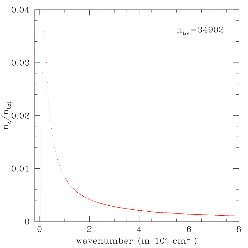
Figure 32: The histogram of the sampling frequency distribution with $n_{\rm tot}=34902$ sampling points, selected following the scheme proposed by Helling & Jørgensen (1998). This represents the reference distribution whence smaller frequency samples are extracted. See the text for more explanation.

Computing the RM opacity with Eq. (2) requires that the total monochromatic absorption coefficient is evaluated at a finite number of frequency points. In principle the more the points, the more accurate the results should be. However, since we are dealing with a mean quantity one can obtain still good results using a relatively low number of frequency points, with the advantage of speeding up the computations.

In respect to this some discussion can be found in Ferguson et al. (2005) who integrate over $24\,000$ points, and Lederer & Aringer (2009) who adopt $5\,645$ points. For the present work we have performed further tests to get useful indications on the relationship between the size of the frequency distribution and quality of the results, in terms of accuracy (reliability) and precision (reproducibility) of the results.

For this purpose we proceed as follows. First, we determine a seed frequency distribution by adopting the scheme proposed by Helling & Jørgensen (1998), originally designed to optimize the selection of frequency points in the OS method. In few words, a frequency distribution produces a correct spectral sampling if it obeys the condition $E_{\tilde{\nu}}(T)\Delta\tilde{\nu}=const.$, i.e. expressing the constancy of the normalized energy density of the Planckian, $E_{\tilde{\nu}}(T)$, over any arbitrary interval $\Delta\tilde{\nu}$, where $\tilde{\nu}$ [cm^-1] is the wave-number. Then, the seeked optimal distribution corresponds to the upper envelope the entire sample of Planckian distributions evaluated at different temperatures, so that we take the maximum of the normalized energy density $E_{\tilde{\nu}}(T)$ at each $\tilde{\nu}$. The final distribution, shown in Fig. 32, is sharply peaked at lower frequencies and declines exponentially at longer frequencies.

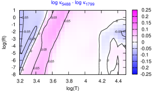
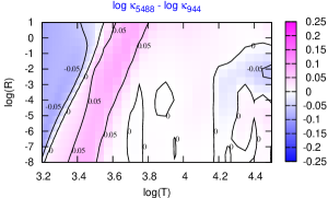
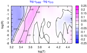
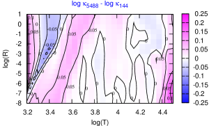
Figure 33: Differences in opacities between the reference frequency grid with $n_{\rm tot}=5488$ points, and other test cases with $n_{\rm tot}=1799,\,944,\,510,\,$ and $149$ points. The adopted chemical composition is characterized by $X=0.7$, $Z_{\rm ref}=0.02$, and scaled-solar abundances according to GS98.

Once the seed distribution is constructed, any other frequency grid of given size is extracted from it by using a Monte-Carlo technique. In our work we tested a few cases adopting 5488, 1799, 944, 510, and 149 points. Each grid is used to compute RM opacities for two chemical compositions characterized by: $I$) $X=0.7$, $Z=Z_{\rm ref}=0.020$ and scaled-solar abundances of metals, and $II$) a carbon-rich mixture with $X=0.7$, $Z_{\rm ref}=0.02$, $Z=0.026$ and C/O $=1.5$. In the latter case carbon is made increase relative to its scaled-solar value, producing a net increment of the actual metallicity.

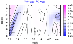
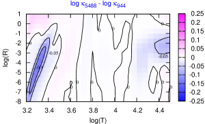
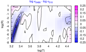
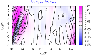
Figure 34: The same as in Fig. 33, but for the adopted chemical composition which is defined by $X=0.7$, $Z_{\rm ref}=0.02$, $Z=0.026$, and C/O $=1.5$.

Then, adopting as reference opacities those obtained with the densest frequency grid, i.e. $n_{\rm tot}=5488$, we evaluate the differences, $\log(\kappa_{4588})-\log(\kappa_{n_{j}})$, for each opacity subset computed with a lower frequency grid (i.e. $n_{j}=1799,\,944,\,510,\,{\rm and}\,149$ points. The results are shown in Fig. 33 for mixture $I$ and Fig. 34 for mixture $II$.

We see that in most cases the differences remain small, within $\simeq\pm 0.05$ dex, over most of the $\log(T)-\log(R)$ space, and even with the smallest frequency set the loss in accuracy, though larger, is not dramatic. As expected, the biggest deviations take place at lower temperatures where the opacity contribution from molecular bands is more sensitive to the frequency sampling.

In any case, it is worth noticing that the uncertainties brought about by the adopted frequency distribution are comparable, if not lower, with the typical differences in RM opacities computed with different codes (see, for instance, Figs. 7 and 18).

Appendix C Chemical mixtures with non-solar $[X_{i}/{\rm Fe}]$ ratios: a general scheme

Let us first consider non-scaled-solar mixtures in which the reference metallicity is preserved, i.e. $Z=Z_{\rm ref}$. Basing on the formalism introduced in Sects.  3.2 and 4.3 we conveniently divide the metal species (with $Z_{i}\geq 3$) into three groups, namely:

• The selected elements with given $\gamma_{i}=[X_{i}^{s}/X_{\rm Fe}]$ according to the input specification, with abundances $X_{i}^{s}=f_{i}^{s}\,X_{i,{\rm ref}}^{s}$;

• The fixed elements with abundances $X_{i}^{f}=X_{i,{\rm ref}}^{f}$;

• The balancing elements, including all the other metals, with abundances $X_{i}^{b}=f_{b}\,X_{i,{\rm ref}}^{b}$.

We recall that the ratios $[X_{i}^{s}/X_{\rm Fe}]$ can be freely chosen to be either positive or negative. According to the adopted scheme, in order to preserve the metallicity the abundance variation of the selected elements should be compensated by the total abundance variation of the balancing elements. It follows that, by construction, all balancing elements share the same variation factor $f^{b}$.

Therefore, from the condition $Z=Z_{\rm ref}$, and the definition of $[X_{i}^{s}/X_{\rm Fe}]$ for each of the $\mathcal{N}_{sel}$ selected elements, we set up a system of $\mathcal{N}_{sel}+1$ equations:

$$\left\{\begin{array}[]{ccl}Z_{\rm ref}&=&\displaystyle\sum_{i}X_{i}^{s}+\displaystyle\sum_{j}X_{j}^{f}+\displaystyle\sum_{k}X_{k}^{b}\\ \displaystyle\left[\frac{X_{i}^{s}}{X_{\rm Fe}}\right]&=&\log\displaystyle\left(\frac{X_{i}^{s}}{X_{\rm Fe}}\right)-\log\displaystyle\left(\frac{X^{s}_{i,\odot}}{X_{\rm Fe,\odot}}\right)\,\,\,\,\,\,\quad\quad\quad\forall\,i=1,\dotsc\mathcal{N}_{sel}\,\,,\end{array}\right.$$

which can be re-formulated with the aid of Eqs. (31) and (34):

$$\left\{\begin{array}[]{ccl}Z_{\odot}&=&\displaystyle\sum_{i}f_{i}^{s}X_{i,\odot}^{s}+\displaystyle\sum_{j}X_{j,\odot}^{f}+f^{b}\,\displaystyle\sum_{k}X_{k,\odot}^{b}\\ 10^{\gamma_{i}}&=&\displaystyle\frac{f_{i}^{s}}{f^{b}}\quad\quad\quad\quad\quad\quad\quad\quad\quad\quad\quad\quad\quad\forall\,i=1,\dotsc\mathcal{N}_{sel}\end{array}\right.$$

for the unknowns $f_{i}^{s}$ and $f^{b}$. Let us denote with

$$\xi_{i,\odot}=\displaystyle\frac{X_{i,\odot}}{Z_{\odot}}$$ (42)

the partitions of metals in the solar mixture. Eventually, from simple analytical passages we obtain the general solution:

$$\left\{\begin{array}[]{ccl}f^{b}&=&\displaystyle\frac{\displaystyle\sum_{i}\xi_{i,\odot}^{s}+\displaystyle\sum_{k}\xi_{k,\odot}^{b}}{\displaystyle\sum_{i}10^{\gamma_{i}}\xi_{i,\odot}^{s}+\displaystyle\sum_{k}\xi_{k,\odot}^{b}}\\ f_{i}^{s}&=&f^{b}\,10^{\gamma_{i}}\quad\quad\quad\quad\quad\quad\quad\quad\quad\forall\,i=1,\dotsc\mathcal{N}_{sel}\end{array}\right.$$ (43)

which only depends on the specified ratios $[X_{i}^{s}/X_{\rm Fe}]$ of the selected elements, and the metal partitions in the reference solar composition. It is useful to particularize Eq. (43) for the cases of mixtures $A$ and $B$ introduced in Sect. 4.3, and finally derive the results for mixture $C$.

Mixture $A$ Since the fixed group is empty, we have $\sum_{i}\xi_{i,\odot}^{s}+\sum_{k}xi_{k,\odot}^{b}=1$, hence:

$$f^{b}=\displaystyle\frac{1}{1+{\displaystyle\sum_{i}(10^{\gamma_{i}}-1)\,\xi_{i,\odot}^{s}}}.$$ (44)

Mixture $B$ Since the balancing elements are those belonging to the Fe-group, i.e. $\sum_{k}X_{k,\odot}^{b}=X_{{\rm Fe},\odot}$, we get:

$$f^{b}=\displaystyle\frac{\displaystyle\sum_{i}\xi_{i,\odot}^{s}+\xi_{{\rm Fe},\odot}}{\displaystyle\sum_{i}10^{\gamma_{i}}\xi_{i,\odot}^{s}+\xi_{{\rm Fe},\odot}}$$ (45)

Mixture $C$ Finally, we consider the case of mixture $C$, in which the reference metallicity $Z_{\rm ref}$ should not be preserved, as the actual metallicity, $Z=f_{Z}Z_{\rm ref}$, follows the total abundance variation of the selected elements. In this case we consider the system of equations

$$\left\{\begin{array}[]{rcl}Z=f_{Z}\,Z_{\rm ref}&=&\displaystyle\sum_{i}X_{i}^{s}+\displaystyle\sum_{j}X_{j}^{non-s}\\ \displaystyle\left[\frac{X_{i}^{s}}{X_{\rm Fe}}\right]&=&\log\displaystyle\left(\frac{X_{i}^{s}}{X_{\rm Fe}}\right)-\log\displaystyle\left(\frac{X^{s}_{i,\odot}}{X_{\rm Fe,\odot}}\right)\,\,\,\quad\quad\quad\forall\,i=1,\dotsc\mathcal{N}_{sel}\,\,,\end{array}\right.$$

where we only distinguish between selected and non-selected elements. From the definitions of the abundance variation factors, recalling that $\sum_{j}X_{j,\odot}^{non-s}=Z_{\odot}-\sum_{i}X_{i,\odot}^{s}$, and after some manipulation, we obtain the equations

$$\left\{\begin{array}[]{ccl}Z_{\odot}&=&\displaystyle\sum_{i}f_{i}^{s}X_{i,\odot}^{s}+\displaystyle\sum_{j}X_{j,\odot}^{non-s}\\ 10^{\gamma_{i}}&=&\displaystyle\frac{f_{i}^{s}}{f^{non-s}}\quad\quad\quad\quad\quad\quad\quad\quad\quad\quad\quad\quad\quad\forall\,i=1,\dotsc\mathcal{N}_{sel}\end{array}\right.$$

for the unknowns $f_{i}^{s}$ and $f^{non-s}$. We notice that formally we deal with exactly the same equations as those for mixture $A$, once the non-selected elements are considered in place of the balancing elements. Hence, the seeked solution is given by Eq. (44) where one substitutes $f^{b}$ with $f^{non-s}$. In other words, mixture $A$ and mixture $C$ share the same non-solar metal partitions $(X_{i}/Z_{\rm ref})_{A}=(X_{i}/Z)_{C}$, but their metallicity is different by a factor $f_{Z}$.