CERN-PH-TH/2009-117

Dark energy, integrated Sachs-Wolfe effect

and large-scale magnetic fields

Massimo Giovannini

Department of Physics, Theory Division, CERN, 1211 Geneva 23, Switzerland INFN, Section of Milan-Bicocca, 20126 Milan, Italy

Abstract

The impact of large-scale magnetic fields on the interplay between the ordinary and integrated Sachs-Wolfe effects is investigated in the presence of a fluctuating dark energy component. The modified initial conditions of the Einstein-Boltzmann hierarchy allow for the simultaneous inclusion of dark energy perturbations and of large-scale magnetic fields. The temperature and polarization angular power spectra are compared with the results obtained in the magnetized version of the (minimal) concordance model. Purported compensation effects arising at large scales are specifically investigated. The fluctuating dark energy component modifies, in a computable manner, the shapes of the $1$- and $2$-$\sigma$ contours in the parameter space of the magnetized background. The allowed spectral indices and magnetic field intensities turn out to be slightly larger than those determined in the framework of the magnetized concordance model where the dark energy fluctuations are absent.

1 Motivations and goals

Defining $z_{{\mathrm{rec}}}=1090.51\pm 0.95$ as the typical redshift of recombination according to the WMAP data alone (see [1, 2] for the 3yr data release and [3, 4, 5, 6, 7] for the 5yr data release) the temperature anisotropies for multipoles $\ell<\sqrt{z_{{\mathrm{rec}}}}$ are practically unaffected by the thickness of the visibility function. The resulting angular power of the temperature inhomogeneities is determined by the ordinary Sachs-Wolfe effect (SW in what follows), by the integrated Sachs-Wolfe effect (ISW effect in what follows) and by their mutual correlation. The origin of the SW and of the ISW contributions is physically distinct. When the opacity drops suddenly, the SW term is determined by the density contrast of the photons and by the curvature perturbations around $z_{{\mathrm{rec}}}$. Conversely the ISW effect depends upon an integral over the conformal time coordinate $\tau$ extending between $\tau_{{\mathrm{rec}}}$ (corresponding to $z_{{\mathrm{rec}}}$) and $\tau_{0}$ (i.e. the present time when $z=0$). The integration path determining the ISW passes through $z_{\Lambda}$, i.e. the redshift at which the dark energy contribution is of the same order of the total density of matter and the geometry starts accelerating. The explicit contribution of the dark energy to the SW and ISW effects (as well as to their cross-correlation) has been scrutinized, for the first time, in [8] (see also [9]) where the effects of the late dominance of a cosmological term have been taken into account in a consistent semi-analytic treatment.

The SW contribution typically peaks for comoving wavenumbers $k\simeq 0.0002\,\mathrm{Mpc}^{-1}$ while the ISW effects contributes between $k_{\mathrm{min}}=0.001\,\mathrm{Mpc}^{-1}$ and $k_{\mathrm{max}}=0.01\,\mathrm{Mpc}^{-1}$. For comparison recall that the angular power spectra of the Cosmic Microwave Background (CMB in what follows) fluctuations are customarily assigned at a pivot scale $k_{\mathrm{p}}=0.002\,\,\mathrm{Mpc}^{-1}$ which corresponds, for the best fit parameters of the WMAP 5yr alone (and in the light of the $\Lambda$CDM scenario) to $\ell_{\mathrm{p}}\simeq 30$. Even if both contributions are reasonably separated in scales, the SW and ISW effects may partially compensate. An effective compensation would imply a suppression of the lowest multipoles (and in particular of the quadrupole) in the angular power spectrum of the temperature autocorrelations. In the context of the $\Lambda$CDM scenario with purely adiabatic fluctuations the compensation is partial and uneffective for the suppression of the quadrupole. If non-adiabatic fluctuations in the dark-energy sector are consistently included, the physical situation is different and a quadrupole suppression cannot be excluded. This possibility has been investigated especially in the context of the (observed) low quadrupole of the temperature autocorrelations [10, 11, 12] (see also [13] for a contending explanations of the same class of phenomena).

The relative contribution of the SW and ISW terms does depend upon the evolution of the background geometry between the recombination epoch and the present time. Furthermore it does also depend upon the potential presence of non-adiabatic fluctuations as well as upon the specific way dark energy is parametrized. In the $\Lambda$CDM paradigm there are, by definition, no fluctuations in the dark energy sector. The rationale for such a statement stems directly from the value of the barotropic index of the dark energy (i.e. $w_{\mathrm{de}}=-1$). The natural extension of the $\Lambda$CDM paradigm to the case when the dark energy fluctuations are dynamical is represented by the $w$CDM model where $w$ stands for the barotropic index of the dark energy component . In the $w$CDM scenario the dark energy fluctuations affect virtually all CMB observables and, more specifically, the best fit parameters will differ from the ones determined, for instance, within the standard $\Lambda$CDM scenario.

A legitimate question concerns, in this context, the role of the large-scale magnetic fields. Indeed the $\Lambda$CDM paradigm served as the simplest framework for the systematic scrutiny of magnetized CMB anisotropies (see, e.g., [14, 15] and [16, 17, 18] for more recent developments). The purpose of the present investigation is to extend the program of [14, 15] by relaxing the hypotheses of [16, 17, 18] on the dark energy component. What happens if the dominant energy density of the background is not parametrized in terms of a cosmological constant and, simultaneously, a magnetized background is present? For large angular separations the interplay between the SW and the ISW effect answers satisfactorily to the previous question, but what happens for higher multipoles? What are the changes in the parameter space of the magnetized background induced by a fluctuating dark energy component?

While there are no doubts that large-scale magnetic fields exist today in nearly all gravitationally bound systems there has been mounting evidence from diverse observations in galaxies [19, 20], clusters [21, 22], superclusters [23], high-redshift quasars [24, 25] that magnetic fields could also have pretty large correlation scales (see [26] for a review on the subject). The evolution of electromagnetic fields in a plasma is subject to daily test in terrestrial laboratories and in astrophysical observations (see, e.g. [27, 28] for historic monographs on the subject). When plasma physics is used to interpret or even justify some astrophysical observations the governing equations are exactly the ones used in terrestrial experiments. This approximation is reasonable for sufficiently small redshift. However, as we move towards higher redshift, the evolution of the space-time curvature cannot be neglected anymore. The spirit of the approach summarized in [16, 17, 18] is to translate the plasma dynamics in flat space-time to a curved background which is the one dictated, for simplicity, by the $\Lambda$CDM paradigm and by its neighboring extensions. Specific attention must be paid, in this respect, to the accurate treatment of the relativistic fluctuations of the geometry and to their initial conditions [14, 15].

The content of the forthcoming sections can be summarized, in short, as follows. In section 2 the governing equations of the system will be introduced. In section 3 the ordinary and integrated SW contributions will be analyzed. Section 4 deals with the initial conditions for the magnetized Einstein-Boltzmann hierarchy in the presence of a fluctuating dark-energy component. In section 5 the numerical aspects of the whole analysis have been collected. Section 6 contains our concluding considerations. Various technical results have been reported in the appendix to avoid excessive digressions from the main logical line of each section.

2 Governing equations

The governing equations of the pre-decoupling plasma can be written in terms of the global magnetohydrodynamical variables, i.e. the total current, the charge density and the baryon velocity (see, e.g. [29]). In most of the astrophysical applications the space-time curvature hardly plays any role in the evolution of the plasma. Prior to decoupling, as already emphasized in section 1, the space-time metric as well its relativistic inhomogeneities are two necessary ingredients for gauging the effects of large-scale magnetism on the CMB observables. The reduction from the two-fluid system to the one-fluid system is discussed in [16, 17, 18] (see, in particular, [29]) with special attention to the effects of the space-time curvature. The magnetohydrodynamical reduction holds, of course under various approximations which are not that dissimilar from the ones usually employed in the case of flat space-time. There are, however, also notable differences which can be summarized as follows:

• since electrons and ions are non-relativistic (i.e. the plasma is cold) the system is not invariant under Weyl rescaling of the space-time metric and this implies that the corresponding evolution equations will be qualitatively different from the case of a non-expanding space-time;

• even if the charge carriers are non-relativistic, the fluctuations of the geometry cannot be treated in the standard Newtonian approximation since the relevant modes of the gravitational field have wavelengths which are larger than the Hubble radius before matter-radiation equality .

With these specifications in mind, the relevant evolution equations will be written prior to decoupling when the electron-photon and electron-ion coupling is still strong.

2.1 Background variables

In a spatially flat background metric of the type $\overline{g}_{\mu\nu}(\tau)=a^{2}(\tau)\eta_{\mu\nu}$ (where $\eta_{\mu\nu}$ is the Minkowski metric) the Friedmann-Lemaître equations take the form

$${\mathcal{H}}^{2}=\frac{8\pi Ga^{2}}{3}\rho_{\mathrm{t}},\qquad{\mathcal{H}}^{2}-{\mathcal{H}}^{\prime}=4\pi Ga^{2}(p_{\mathrm{t}}+\rho_{\mathrm{t}}),\qquad{\mathcal{H}}=\frac{a^{\prime}}{a},$$ (2.1)

where the prime denotes a derivation with respect to the conformal time coordinate $\tau$. The explicit form of the energy density and of the enthalpy density appearing in Eq. (2.1) is given by:

$$\rho_{\mathrm{t}}=\rho_{\mathrm{e}}+\rho_{\mathrm{i}}+\rho_{\mathrm{c}}+\rho_{\gamma}+\rho_{\nu}+\rho_{\mathrm{de}},$$ (2.2)

$$\rho_{\mathrm{t}}+p_{\mathrm{t}}=\frac{4}{3}(\rho_{\nu}+\rho_{\gamma})+\rho_{\mathrm{c}}+\rho_{\mathrm{e}}+\rho_{\mathrm{i}}+(w_{\mathrm{de}}+1)\rho_{\mathrm{de}}.$$ (2.3)

In the one-fluid limit the electron and ion energy densities form a single physical entity, i.e. the baryonic matter density $\rho_{\mathrm{b}}=\rho_{\mathrm{e}}+\rho_{\mathrm{i}}$ where $\rho_{\mathrm{e}}=m_{\mathrm{e}}n_{0}$ and $\rho_{\mathrm{i}}=m_{\mathrm{i}}n_{0}$ are, respectively, the electron and ion matter densities. The comoving concentrations of electrons and ions (i.e. $n_{0}=a^{3}\tilde{n}_{0}$) coincide because of the electric neutrality of the plasma . The remaining energy densities in Eqs. (2.2) and (2.3) parametrize the contributions of neutrinos (with subscript $\nu$), of photons (with subscript $\gamma$), of cold dark matter particles (with subscript c); finally $\rho_{\mathrm{de}}$ denotes the dark energy density while $w_{\mathrm{de}}$, as already mentioned, is the barotropic index of dark energy.

2.2 Fluctuations of the geometry

Diverse gauges lead to slightly different (but mathematically equivalent) physical pictures of the effects discussed in the present investigation. To avoid a pedantic presentation, the relevant equations will be swiftly introduced in the conformally Newtonian gauge with the proviso that the very same equations will be expressed, when needed, in the synchronous frame. The recipe to move between these two gauges will now be given together with the appropriate definitions of the perturbed line elements. In the conformally Newtonian gauge the perturbed entries of the metric are given by:

$$\delta^{(\mathrm{cn})}_{\mathrm{s}}g_{00}(k,\tau)=2a^{2}(\tau)\phi(k,\tau),\qquad\delta^{(\mathrm{cn})}_{\mathrm{s}}g_{ij}(k,\tau)=2a^{2}(\tau)\psi(k,\tau)\delta_{ij};$$ (2.4)

while in the synchronous gauge the perturbed metric can be written as:

$$\delta^{(\mathrm{S})}_{\mathrm{s}}g_{ij}(k,\tau)=a^{2}(\tau)\biggl{[}\hat{k}_{i}\hat{k}_{j}\,h(k,\tau)+6\,\xi(k,\tau)\,\biggl{(}\hat{k}_{i}\hat{k}_{j}-\frac{\delta_{ij}}{3}\biggr{)}\biggr{]},$$ (2.5)

where $\hat{k}_{i}=k_{i}/|\vec{k}|$. The parametrizations of Eqs. (2.4) and (2.5) are related by the appropriate coordinate transformations, i.e.

$$\psi(k,\tau) = -\xi(k,\tau)+\frac{{\mathcal{H}}}{2k^{2}}[h(k,\tau)+6\xi(k,\tau)]^{\prime},$$

$$\phi(k,\tau) = -\frac{1}{2k^{2}}\{[h(k,\tau)+6\xi(k,\tau)]^{\prime\prime}+{\mathcal{H}}[h(k,\tau)+6\xi(k,\tau)]^{\prime}\}.$$ (2.6)

Consider, for instance, the curvature perturbations on comoving orthogonal hypersurfaces, i.e. ${\mathcal{R}}(k,\tau)$, within the description provided by the conformally Newtonian gauge:

$${\mathcal{R}}(k,\tau)=-\psi-\frac{{\mathcal{H}}({\mathcal{H}}\phi+\psi^{\prime})}{{\mathcal{H}}^{2}-{\mathcal{H}}^{\prime}}\to\xi+\frac{{\mathcal{H}}\xi^{\prime}}{{\mathcal{H}}^{2}-{\mathcal{H}}^{\prime}},$$ (2.7)

where the arrow simply labels the coordinate transformation from the conformally Newtonian gauge to the synchronous coordinate system; the last expression in Eq. (2.7) is obtained by shifting metric fluctuations according to Eq. (2.6). From the last equality in Eq. (2.7) it is also apparent that when ${\mathcal{R}}^{\prime}=0$, $\xi(k)={\mathcal{R}}(k)$. In more general terms, by solving Eq. (2.7) in terms of $\xi$, it can be shown, after integration by part, that

$$\xi(k,\tau)={\mathcal{R}}(k,\tau)-\frac{{\mathcal{H}}(\tau)}{a(\tau)}\int_{0}^{\tau}\frac{a(\tau_{1})}{{\mathcal{H}}(\tau_{1})}{\mathcal{R}}^{\prime}(k,\tau_{1})\,d\tau_{1},$$ (2.8)

where $\tau_{1}$ is an integration variable and where the prime denotes, as usual, a derivation with respect to $\tau$. Both in analytical and numerical calculations the normalization of the curvature perturbations is customarily expressed in terms of ${\mathcal{R}}$; for this reason Eqs. (2.7) and (2.8) turn out to be particularly useful in the explicit estimates. The same transformations of Eq. (2.6) can be used to gauge-transform the governing equations from the conformally Newtonian farme to the synchronous coordinate system. Equation (2.8) also justifies, a posteriori, the perturbed form of the line element introduced in Eq. (2.5): the factor of $6$ in front of $\xi$ is essential if we want $\xi(k,\tau)$ to coincide with ${\mathcal{R}}(k,\tau)$ at least in the case of the adiabatic mode when ${\mathcal{R}}_{*}(k)$ does not depend on time prior to equality and for wavelengths larger than the Hubble radius.

The present conventions as well as the whole approach slightly differ from the treatment of, for instance, Ref. [30] (see also [31]). In the present approach the curvature perturbations on comoving orthogonal hypersurfaces (i.e. ${\mathcal{R}}$) are simply related, in the large-scale limit, to the curvature perturbations on uniform density hypersurfaces (see, e.g. [32] and also [33, 34]). From the latter observations, most of the synchronous gauge results needed in the present analysis follow by making judicious use of Eq. (2.8). The need for the synchronous description is also motivated since the code used for present numerical analysis is based, originally, on COSMICS [35] and on CMBFAST [36, 37]. The numerical code used here is an extension of what has been described and exploited in [16, 17, 18]. It is also worth mentioning, for completeness, that there exist approaches to cosmological perturbations which are fully covariant [38] and which have been also applied to the case of large-scale magnetic fields [39] without leading, in the latter case, to any explicit estimate or of the temperature and polarization angular power spectra neither in the $\Lambda$CDM paradigm nor in its neighboring extensions such as the ones analyzed in the present paper.

2.3 Evolution equations for the inhomogenities

The Hamiltonian and momentum constraints stemming, respectively, from the $(00)$ and $(0i)$ (perturbed) Einstein equations are given, in real space, by

$$\nabla^{2}\psi-3{\mathcal{H}}({\mathcal{H}}\phi+\psi^{\prime})=4\pi Ga^{2}[\delta_{\mathrm{s}}\rho_{\mathrm{f}}+\delta_{\mathrm{s}}\rho_{\mathrm{de}}+\delta_{\mathrm{s}}\rho_{\mathrm{B}}+\delta_{\mathrm{s}}\rho_{\mathrm{E}}],$$ (2.9)

$$\vec{\nabla}({\mathcal{H}}\phi+\psi^{\prime})=-4\pi Ga^{2}\biggl{[}(p_{\mathrm{t}}+\rho_{\mathrm{t}})\vec{v}_{\mathrm{t}}+\frac{\vec{E}\times\vec{B}}{4\pi}\biggr{]},$$ (2.10)

where, $\delta_{\mathrm{s}}\rho_{\mathrm{f}}=\delta_{\mathrm{s}}\rho_{\mathrm{b}}+\delta_{\mathrm{s}}\rho_{\mathrm{c}}+\delta_{\mathrm{s}}\rho_{\nu}+\delta_{\mathrm{s}}\rho_{\gamma}$ is the density fluctuation of the fluid sources in the longitudinal gauge. In Eq. (2.10) the total velocity field $\vec{v}_{\mathrm{t}}$ obeys

$$(p_{\mathrm{t}}+\rho_{\mathrm{t}})\vec{v}_{\mathrm{t}}=\frac{4}{3}\rho_{\nu}\vec{v}_{\nu}+\frac{4}{3}\rho_{\gamma}(1+R_{\mathrm{b}})\vec{v}_{\gamma\mathrm{b}}+\rho_{\mathrm{c}}\vec{v}_{\mathrm{c}}+(w_{\mathrm{de}}+1)\rho_{\mathrm{de}}\vec{v}_{\mathrm{de}};$$ (2.11)

as already mentioned $w_{\mathrm{de}}$ is the barotropic index of the dark energy component i.e.

$$w_{\mathrm{de}}=\frac{p_{\mathrm{de}}}{\rho_{\mathrm{de}}},\qquad c_{\mathrm{s\,de}}^{2}=w_{\mathrm{de}}-\frac{w_{\mathrm{de}}^{\prime}}{3{\mathcal{H}}(w_{\mathrm{de}}+1)},$$ (2.12)

where the sound speed of dark energy has been also introduced. In Eq. (2.11) $R_{\mathrm{b}}=3\rho_{\mathrm{b}}/(4\rho_{\gamma})$ denotes the baryon to photon ratio. Prior to photon decoupling the baryon and photon velocities effectively coincide with $\vec{v}_{\gamma\mathrm{b}}$

$$\vec{v}_{\gamma\mathrm{b}}\simeq\vec{v}_{\gamma}\simeq\vec{v}_{\mathrm{b}},\qquad\vec{v}_{\mathrm{b}}=\frac{m_{\mathrm{e}}\vec{v}_{\mathrm{e}}+m_{\mathrm{i}}\vec{v}_{\mathrm{i}}}{m_{\mathrm{e}}+m_{\mathrm{i}}}.$$ (2.13)

In Eqs. (2.9) and (2.10) the gravitational effects of the large-scale electromagnetic fields have been included in terms of the comoving electric and magnetic fields $\vec{E}(\vec{x},\tau)=a^{2}(\tau)\vec{{\mathcal{E}}}(\vec{x},\tau)$ and $\vec{B}(\vec{x},\tau)=a^{2}(\tau)\vec{{\mathcal{B}}}(\vec{x},\tau)$, i.e.

$$\delta_{\mathrm{s}}\rho_{\mathrm{B}}=\frac{B^{2}}{8\pi a^{4}},\qquad\delta_{\mathrm{s}}\rho_{\mathrm{E}}=\frac{E^{2}}{8\pi a^{4}},\qquad\delta_{\mathrm{s}}p_{\mathrm{B}}=\frac{\delta_{\mathrm{s}}\rho_{\mathrm{B}}}{3},\qquad\delta_{\mathrm{s}}p_{\mathrm{E}}=\frac{\delta_{\mathrm{s}}\rho_{\mathrm{E}}}{3},$$ (2.14)

where $B^{2}=|\vec{B}|^{2}$ and $E^{2}=|\vec{E}|^{2}$. The evolution equations for $\vec{E}$ and $\vec{B}$ are:

$$\vec{\nabla}\cdot\vec{B}=0,\qquad\vec{\nabla}\cdot\vec{E}=4\pi\rho_{\mathrm{q}},$$ (2.15)

$$\vec{\nabla}\times\vec{E}+\vec{B}^{\prime}=0,\qquad\vec{\nabla}\times\vec{B}=4\pi\vec{J}+\vec{E}^{\prime}$$ (2.16)

$$\rho_{\mathrm{q}}^{\prime}+\vec{\nabla}\cdot\vec{J}=0,\qquad\rho_{\mathrm{q}}=e(n_{\mathrm{i}}-n_{\mathrm{e}}),\qquad\vec{J}=e(n_{\mathrm{i}}\vec{v}_{\mathrm{i}}-n_{\mathrm{e}}\vec{v}_{\mathrm{e}}).$$ (2.17)

The total current $\vec{J}$ has been expressed in terms of the two fluid variables, however, as in the case of flat-space magnetohydrodynamics, $\vec{J}$ can be related to the electromagnetic fields by means of the generalized Ohm law [29]:

$$\vec{J}=\sigma\biggl{(}\vec{E}+\vec{v}_{\mathrm{b}}\times\vec{B}+\frac{\vec{\nabla}p_{\mathrm{e}}}{e\,n_{0}}-\frac{\vec{J}\times\vec{B}}{n_{0}e}\biggr{)},\qquad\sigma=\frac{\omega_{\mathrm{pe}}^{2}}{4\pi\{a\Gamma_{\mathrm{ie}}+(4/3)[\rho_{\gamma}/(n_{0}m_{\mathrm{e}})]\Gamma_{\mathrm{e}\gamma}\}},$$ (2.18)

where $\sigma$ is the conductivity; $\Gamma_{\mathrm{ie}}$ and $\Gamma_{\gamma\mathrm{e}}$ are, respectively, the electron-ion and electron-photon interaction rates. The three terms appearing in the Ohm’s law are, besides the electric field, the drift term (i.e. $\vec{v}_{\mathrm{b}}\times\vec{B}$), the thermoelectric term (containing the gradient of the electron pressure) and the Hall term (i.e. $\vec{J}\times\vec{B}$). It can be shown [29] that for frequencies much smaller than the (electron) plasma frequency and for typical length-scales much larger than the Debye screening length the Hall and thermoelectric terms are subleading for the purposes of the present analysis. The electromagnetic pressure as well as the anisotropic stresses enter the perturbed $(ij)$ components of the Einstein equations:

$$\psi^{\prime\prime}+{\mathcal{H}}(\phi^{\prime}+2\psi^{\prime})+({\mathcal{H}}^{2}+2{\mathcal{H}}^{\prime})\phi$$

$$+\frac{1}{3}\nabla^{2}(\phi-\psi)=4\pi Ga^{2}[\delta_{\mathrm{s}}p_{\mathrm{f}}+\delta_{\mathrm{s}}p_{\mathrm{de}}+\delta_{\mathrm{s}}p_{\mathrm{B}}+\delta p_{\mathrm{E}}],$$ (2.19)

$$\nabla^{4}(\phi-\psi)=16\pi Ga^{2}\biggl{[}\rho_{\nu}\nabla^{2}\sigma_{\nu}+\rho_{\gamma}\nabla^{2}\sigma_{\mathrm{B}}+\rho_{\gamma}\nabla^{2}\sigma_{\mathrm{E}}+\frac{3}{4}\rho_{\mathrm{de}}(w_{\mathrm{de}}+1)\nabla^{2}\sigma_{\mathrm{de}}\biggr{]},$$ (2.20)

where $\delta_{\mathrm{s}}p_{\mathrm{f}}=(\delta_{\mathrm{s}}\rho_{\gamma}+\delta_{\mathrm{s}}\rho_{\nu})/3$, in analogy with $\delta_{\mathrm{s}}\rho_{\mathrm{f}}$, denotes the fluctuation of the pressure of the fluid components. The total anisotropic stress is given, as usual, by

$$\Pi_{i\,\mathrm{t}}^{j}=\Pi_{i\,\nu}^{j}+\Pi_{i\,\mathrm{B}}^{j}+\Pi_{i\,\mathrm{E}}^{j}+\Pi_{i\,\mathrm{de}}^{j};$$ (2.21)

the various subscripts denote the respective components and, in particular the electromagnetic contribution:

$$\Pi_{i\,\mathrm{B}}^{j}=\frac{1}{4\pi a^{4}}\biggl{[}B_{i}B^{j}-\frac{\delta_{i}^{j}}{3}B^{2}\biggr{]},\qquad\Pi_{i\,\mathrm{E}}^{j}=\frac{1}{4\pi a^{4}}\biggl{[}E_{i}E^{j}-\frac{\delta_{i}^{j}}{3}E^{2}\biggr{]}.$$ (2.22)

In Eq. (2.20) the notation

$$\partial_{i}\partial_{j}\Pi^{ij}_{\mathrm{t}}=\frac{4}{3}\rho_{\nu}\nabla^{2}\sigma_{\nu}+\frac{4}{3}\rho_{\gamma}\nabla^{2}\sigma_{\mathrm{B}}+\frac{4}{3}\rho_{\gamma}\nabla^{2}\sigma_{\mathrm{E}}+\rho_{\mathrm{de}}(w_{\mathrm{de}}+1)\nabla^{2}\sigma_{\mathrm{de}},$$ (2.23)

has been adopted. The various species of the plasma either interact strongly with the plasma (like the elctrons, the ions and the photons) or they only feel the effects of the geometry (like the CDM component and the dark-energy). For large-scales the baryon-photon system obeys

$$\delta_{\mathrm{b}}^{\prime}=3\psi^{\prime}-\theta_{\mathrm{b}},$$ (2.24)

$$\theta_{\mathrm{b}}^{\prime}+{\mathcal{H}}\theta_{\mathrm{b}}^{\prime}=\frac{\vec{\nabla}\cdot[\vec{J}\times\vec{B}]}{a^{4}\rho_{\mathrm{b}}}-\nabla^{2}\phi+\frac{4}{3}\frac{\rho_{\gamma}}{\rho_{\mathrm{b}}}\epsilon^{\prime}(\theta_{\gamma}-\theta_{\mathrm{b}}),$$ (2.25)

$$\theta_{\gamma}^{\prime}=-\frac{1}{4}\nabla^{2}\delta_{\gamma}-\nabla^{2}\phi+\epsilon^{\prime}(\theta_{\mathrm{b}}-\theta_{\gamma}),$$ (2.26)

$$\delta_{\gamma}^{\prime}=4\psi^{\prime}-\frac{4}{3}\theta_{\gamma},$$ (2.27)

where $\epsilon^{\prime}$ is the differential optical depth; furthermore, defining as $\vec{v}_{X}$ the velocity of the species $X$, $\theta_{X}=\vec{\nabla}\cdot\vec{v}_{X}$. The CDM and the neutrino components will evolve, respectively, as

$$\delta_{\mathrm{c}}^{\prime}=3\psi^{\prime}-\theta_{\mathrm{c}},$$ (2.28)

$$\theta_{\mathrm{c}}^{\prime}+{\mathcal{H}}\theta_{\mathrm{c}}=-\nabla^{2}\phi,$$ (2.29)

and as

$$\theta_{\nu}^{\prime}=-\frac{1}{4}\nabla^{2}\delta_{\nu}+\nabla^{2}\sigma_{\nu}-\nabla^{2}\phi,$$ (2.30)

$$\delta_{\nu}^{\prime}=4\psi^{\prime}-\frac{4}{3}\theta_{\nu},$$ (2.31)

$$\sigma_{\nu}^{\prime}=\frac{4}{15}\theta_{\nu}-\frac{3}{10}{\mathcal{F}}_{\nu 3},$$ (2.32)

where ${\mathcal{F}}_{\nu 3}$ reminds of the coupling of the monopole and of the dipole to the higher multipoles of the neutrino phase space distribution. The latter term will be set to zero in the class of initial conditions discussed in the present paper but it can be relevant when magnetized non-adiabatic modes are consistently included. The fluctuations of the dark energy density obey, in the $w$CDM scenario, the following equation:

$$\delta_{\mathrm{s}}\rho_{\mathrm{de}}^{\prime}+3{\mathcal{H}}(\delta_{\mathrm{s}}\rho_{\mathrm{de}}+\delta p_{\mathrm{de}})-3\psi^{\prime}(p_{\mathrm{de}}+\rho_{\mathrm{de}})+(\rho_{\mathrm{de}}+p_{\mathrm{de}})\vec{\nabla}\cdot\vec{v}_{\mathrm{de}}=0,$$ (2.33)

where, as already mentioned, $\vec{v}_{\mathrm{de}}$ is the velocity of the dark energy in the conformally Newtonian frame whose evolution equation can be written as

$$(p_{\mathrm{de}}+\rho_{\mathrm{de}})\vec{v}_{\mathrm{de}}^{\prime}+[p_{\mathrm{de}}^{\prime}+\rho_{\mathrm{de}}^{\prime}+4{\mathcal{H}}(p_{\mathrm{de}}+\rho_{\mathrm{de}})]\vec{v}_{\mathrm{de}}+\vec{\nabla}\delta p_{\mathrm{de}}$$

$$+(p_{\mathrm{de}}+\rho_{\mathrm{de}})\vec{\nabla}\phi-(p_{\mathrm{de}}+\rho_{\mathrm{de}})\vec{\nabla}\sigma_{\mathrm{de}}=0.$$ (2.34)

In Eq. (2.34) $\sigma_{\mathrm{de}}$ accounts for the possible presence of an anisotropic stress for the dark energy contribution. This contribution as argued in [40] (see also, in a related perspective, [41]) can be rather interesting in connection with dark energy models. The contribution of the dark energy anisotropic stress has been included, so far, to have sufficiently general equations. In the standard version of the wCDM scenario the dark energy has no anisotropic stress and therefore, for practical reasons, the anisotropic stress will be set to zero. It might be interesting, in the future, to relax this assumption by following, for instance, the approach of [40]. By introducing the density contrast for the dark energy component, Eqs. (2.33) and (2.34) can also be written as

$$\delta_{\mathrm{de}}^{\prime}+3{\mathcal{H}}(c_{\mathrm{s\,de}}^{2}-w_{\mathrm{de}})\delta_{\mathrm{de}}+(w_{\mathrm{de}}+1)\theta_{\mathrm{de}}-3(w_{\mathrm{de}}+1)\psi^{\prime}=0,$$ (2.35)

$$\theta_{\mathrm{de}}^{\prime}+{\mathcal{H}}(1-3c_{\mathrm{s\,de}}^{2})\theta_{\mathrm{de}}+\frac{c_{\mathrm{s\,de}}^{2}\nabla^{2}\delta_{\mathrm{de}}}{(w_{\mathrm{de}}+1)}+\nabla^{2}\phi-\nabla^{2}\sigma_{\mathrm{de}}=0,$$ (2.36)

where $\theta_{\mathrm{de}}=\vec{\nabla}\cdot\vec{v}_{\mathrm{de}}$ and $\delta_{\mathrm{s}}\rho_{\mathrm{de}}=\rho_{\mathrm{de}}\delta_{\mathrm{de}}$. The governing equations can be easily translated in the synchronous coordinate system (see, in particular, Eqs. (2.4), (2.5) and (2.6)–(2.8)). For instance the synchronous form of Eq. (2.9) can be obtained by using, directly, Eqs. (2.4) and (2.5) and by appreciating that

$$\delta^{(\mathrm{cn})}_{\mathrm{s}}\rho_{\mathrm{f}}=\delta^{(\mathrm{S})}_{\mathrm{s}}\rho_{\mathrm{f}}-\rho_{\mathrm{f}}^{\prime}\frac{(h^{\prime}+6\xi^{\prime})}{2k^{2}},\qquad\delta^{(\mathrm{cn})}_{\mathrm{s}}\rho_{\mathrm{de}}=\delta^{(\mathrm{S})}_{\mathrm{s}}\rho_{\mathrm{de}}-\rho_{\mathrm{de}}^{\prime}\frac{(h^{\prime}+6\xi^{\prime})}{2k^{2}}.$$ (2.37)

Since $\rho_{\mathrm{f}}=(\rho_{\gamma}+\rho_{\nu}+\rho_{\mathrm{c}}+\rho_{\mathrm{b}})$ and $\rho_{\mathrm{de}}$ are separately conserved (i.e. $\rho_{\mathrm{f}}^{\prime}=-3{\mathcal{H}}(\rho_{\mathrm{f}}+p_{\mathrm{f}})$ and $\rho_{\mathrm{de}}^{\prime}=-3{\mathcal{H}}(\rho_{\mathrm{de}}+p_{\mathrm{de}})$) the result will be, as expected:

$$2k^{2}\xi-{\mathcal{H}}h^{\prime}=8\pi Ga^{2}[\delta^{(\mathrm{S})}_{\mathrm{s}}\rho_{\mathrm{f}}+\delta^{(\mathrm{S})}_{\mathrm{s}}\rho_{\mathrm{de}}+\delta^{(\mathrm{S})}_{\mathrm{s}}\rho_{\mathrm{B}}+\delta^{(\mathrm{S})}_{\mathrm{s}}\rho_{\mathrm{E}}].$$ (2.38)

In the same way all the other governing equations reported in this sections can be translated in the synchronous frame.

2.4 Large-scale evolution

The Hamiltonian constraint of Eq. (2.9) can be expressed as

$$\zeta={\mathcal{R}}+\frac{\nabla^{2}\psi}{12\pi Ga^{2}(p_{\mathrm{t}}+\rho_{\mathrm{t}})},$$ (2.39)

where ${\mathcal{R}}$ has been introduced in Eq. (2.7) and $\zeta$ [18] (see also [33, 34]) is a further gauge-invariant variable which measures the density contrast on uniform curvature hypersurfaces. The constraint (2.39) can also be used as an explicit definition of $\zeta$ whose evolution depends also upon the gravitating effects of the electromagnetic fields and of the Ohmic current [29]

$$\frac{\partial\zeta}{\partial\tau} = -\frac{{\mathcal{H}}\,\delta p_{\mathrm{nad}}}{p_{\mathrm{t}}+\rho_{\mathrm{t}}}+\frac{{\mathcal{H}}(3\,c_{\mathrm{st}}^{2}-1)}{3(p_{\mathrm{t}}+\rho_{\mathrm{t}})}\delta_{\mathrm{s}}\rho_{\mathrm{B}}$$ (2.40)

$$+ \frac{\vec{E}\cdot\vec{J}}{3a^{4}(p_{\mathrm{t}}+\rho_{\mathrm{t}})}+\frac{\delta_{\mathrm{s}}\rho_{\mathrm{E}}^{\prime}+3(c_{\mathrm{st}}^{2}+1){\mathcal{H}}\delta_{\mathrm{s}}\rho_{\mathrm{E}}}{3(p_{\mathrm{t}}+\rho_{\mathrm{t}})}-\frac{\theta_{\mathrm{t}}}{3},$$

$$\frac{\partial\vec{J}}{\partial\tau} = -\biggl{(}{\mathcal{H}}+a\Gamma_{\mathrm{ie}}-\frac{4\rho_{\gamma}\Gamma_{\mathrm{e}\gamma}}{3n_{0}\,m_{\mathrm{e}}}\biggr{)}\vec{J}$$ (2.41)

$$+ \frac{\omega_{\mathrm{pe}}^{2}}{4\pi}\biggl{(}\vec{E}+\vec{v}_{\mathrm{b}}\times\vec{B}+\frac{\vec{\nabla}p_{\mathrm{e}}}{e\,n_{0}}-\frac{\vec{J}\times\vec{B}}{en_{0}}\biggr{)}+\frac{4e\rho_{\gamma}\Gamma_{\mathrm{e}\gamma}}{3m_{\mathrm{e}}}(\vec{v}_{\mathrm{b}}-\vec{v}_{\gamma}).$$

In Eq. (2.40) the contribution of non-adiabatic pressure fluctuations has been included for sake of completeness even if $\delta p_{\mathrm{nad}}$ will not play a specific role. One of the possible extensions of the present work could indeed be the inclusion of non-adiabatic modes in the dark-energy sector (as argued, for instance, in [10] in connection with the problem of the quadrupole suppression). In connection with Eqs. (2.39), (2.40) and (2.41) few remarks are in order:

• since both $\zeta$ and ${\mathcal{R}}$ are invariant under gauge transformations, they do coincide, in any frame, in the limit $k\ll{\mathcal{H}}$;

• the right hand side of Eq. (2.40) contains three qualitatively different contributions: the purely electric contribution (proportional to $\delta_{\mathrm{s}}\rho_{\mathrm{E}}$ and its derivative), the purely magnetic contribution (proportional to $\delta_{\mathrm{s}}\rho_{\mathrm{B}}$) and the Ohmic contribution (containing explicitly the Ohmic current $\vec{J}$);

• the factor $\theta_{\mathrm{t}}$ at the right hand side of Eq. (2.40) is of order $k^{2}/{\mathcal{H}}$ and it is subleading for typical length-scales larger than the Hubble radius;

• Eq. (2.42) reduces, at large scales, to Eq. (2.18): this statement can be directly verified by taking into account that the rate of electron-ion interactions (i.e. $\Gamma_{\mathrm{ie}}$) is always much larger than the rate of electron-photon interaction (i.e. $\Gamma_{\gamma\mathrm{e}}$); prior to decoupling both $\Gamma_{\mathrm{ie}}$ and $\Gamma_{\gamma\mathrm{e}}$ are larger than ${\mathcal{H}}$.

The physical hierarchies between the electric, magnetic and Ohmic contributions follow from the typical length-scales of the problem and also from the frequency range dictated by the magnetohydrodynamical approximation (see [29] and, in particular, the left plot of Fig.1):

$$\frac{\delta_{\mathrm{s}}\rho_{\mathrm{E}}^{\prime}}{(p_{\mathrm{t}}+\rho_{\mathrm{t}})}<{\mathcal{H}}\delta_{\mathrm{s}}\rho_{\mathrm{E}}\ll\frac{\vec{E}\cdot\vec{J}}{a^{4}(p_{\mathrm{t}}+\rho_{\mathrm{t}})}\ll\frac{{\mathcal{H}}\delta_{\mathrm{s}}\rho_{\mathrm{B}}}{(p_{\mathrm{t}}+\rho_{\mathrm{t}})}.$$ (2.42)

The magnetic contribution appearing at the right hand side of Eq. (2.40) can also be written as

$$\frac{{\mathcal{H}}(3c_{\mathrm{st}}^{2}-1)}{3(1+w_{\mathrm{t}})}\frac{\rho_{\mathrm{R}}}{\rho_{\mathrm{t}}}R_{\gamma}\Omega_{\mathrm{B}},\qquad R_{\gamma}+R_{\nu}=1,$$ (2.43)

where $R_{\nu}=0.405$ and $R_{\gamma}=0.595$ are, respectively, the photon and neutrino fractions present in the radiation plasma and

$$\Omega_{\mathrm{B}}(\vec{x},\tau)=\frac{\delta_{\mathrm{s}}\rho_{\mathrm{B}}(\vec{x},\tau)}{\rho_{\gamma}(\tau)}.$$ (2.44)

Recalling the parametrization of the anisotropic stress $\sigma_{\mathrm{B}}$, the divergence of the magnetohydrodynamical Lorentz force, i.e. $\vec{\nabla}\cdot[\vec{J}\times\vec{B}]$ can be expressed as a combination of $\nabla^{2}\sigma_{\mathrm{B}}$ and $\nabla^{2}\Omega_{\mathrm{B}}$. These vector identities are important in various analytic estimates (see [16, 17, 18] and discussions therein). In the case where the dark energy is simply given by the cosmological constant the total barotropic index and the total sound speed can be written as:

$$w_{\mathrm{t}}=\frac{p_{\mathrm{t}}}{\rho_{\mathrm{t}}}=\frac{1-3\frac{\alpha^{4}}{\alpha_{\Lambda}^{3}}}{3(1+\alpha+\frac{\alpha^{4}}{\alpha_{\Lambda}^{3}})},\qquad c_{\mathrm{st}}^{2}=\frac{p_{\mathrm{t}}^{\prime}}{\rho_{\mathrm{t}}^{\prime}}=w_{\mathrm{t}}-\frac{\alpha}{3(1+w_{\mathrm{t}})}\frac{\partial w_{\mathrm{t}}}{\partial\alpha}=\frac{4}{3(3\alpha+4)},$$ (2.45)

where $\alpha=a/a_{\mathrm{eq}}$ and

$$\alpha_{\Lambda}=\frac{a_{\Lambda}}{a_{\mathrm{eq}}}=2246.81\biggl{(}\frac{h_{0}^{2}\Omega_{\mathrm{M}0}}{0.1326}\biggr{)}^{4/3}\biggl{(}\frac{h_{0}^{2}\Omega_{\Lambda}}{0.3835}\biggr{)},\qquad\alpha_{0}=3195.18\,\biggl{(}\frac{h_{0}^{2}\Omega_{\mathrm{M}0}}{0.1326}\biggr{)}.$$ (2.46)

Using Eqs. (2.45) into Eq. (2.43) we also have, in Fourier space,

$$\frac{{\mathcal{H}}(3c_{\mathrm{st}}^{2}-1)}{3(1+w_{\mathrm{t}})}\frac{\rho_{\mathrm{R}}}{\rho_{\mathrm{t}}}R_{\gamma}\Omega_{\mathrm{B}}(k)=-\frac{3\alpha}{(3\alpha+4)^{2}}R_{\gamma}\Omega_{\mathrm{B}}(k).$$ (2.47)

3 Large-scale compensations

The evolution of the brightness perturbations can be written as :

$$\Delta_{\mathrm{I}}^{\prime}+(ik\mu+\epsilon^{\prime})\Delta_{\mathrm{I}}=\psi^{\prime}-ik\mu\phi+\epsilon^{\prime}\biggl{[}\Delta_{\mathrm{I}0}+\mu v_{\mathrm{b}}+\frac{(1-3\mu^{2})}{4}S_{\mathrm{P}}(k,\tau)\biggl{]},$$ (3.1)

where $S_{\mathrm{P}}$ can be expressed as the sum of the quadrupole of the intensity, of the monopole of the polarization and of the quadrupole of the polarization, i.e., respectively, $S_{\mathrm{P}}(k,\tau)=(\Delta_{\mathrm{I}2}+\Delta_{\mathrm{P}0}+\Delta_{\mathrm{P}2})$. The multipole expansion of the brightness perturbation reads, within the present conventions,

$$\Delta_{\mathrm{I}}(k,\mu,\tau_{0})=\sum_{\ell}(-i)^{\ell}(2\ell+1)\Delta_{\mathrm{I}\ell}(k,\tau_{0})P_{\ell}(\mu),$$ (3.2)

where $P_{\ell}(\mu)$ are the standard Legendre polynomials. The line of sight solution of Eq. (3.1) can be written

$$\Delta_{\mathrm{I}}(k,\mu,\tau_{0}) = \int_{0}^{\tau_{0}}{\mathcal{K}}(\tau)\biggl{[}\Delta_{\mathrm{I}0}+\phi+\mu v_{\mathrm{b}}+\frac{(1-3\mu^{2})}{4}S_{\mathrm{P}}\biggr{]}e^{-i\mu x(\tau)}$$ (3.3)

$$+ \int_{0}^{\tau_{0}}d\tau e^{-\epsilon(\tau,\tau_{0})}(\phi^{\prime}+\psi^{\prime})e^{-i\mu x(\tau)}d\tau,\qquad{\mathcal{K}}(\tau)=\epsilon^{\prime}e^{-\epsilon(\tau,\tau_{0})},$$

where the term $-ik\mu\phi$ has been integrated by parts and where ${\mathcal{K}}(\tau)$ denotes the visibility function whose explicit form can be approximated by a Gaussian profile [42, 43, 44, 45] with different methods. At large scales the Gaussian can be considered effectively a Dirac delta function approximately centered at recombination.

For typical multipoles $\ell\leq\sqrt{z_{\mathrm{rec}}}$ the finite width of the visibility function is immaterial. This means that for sufficiently small $\ell$ everything goes as if the opacity suddenly drops at recombination. This implies that the visibility function presents a sharp (i.e. infinitely thin peak at the recombination time). Thus, since ${\mathcal{K}}(\tau)$ is proportional to a Dirac delta function and $e^{-\epsilon(\tau,\tau_{0})}$ is proportional to an Heaviside theta function. Under the latter approximations, Eq. (3.3) leads to the wanted separation between SW and ISW contributions:

$$\Delta_{\mathrm{I}}(k,\mu,\tau_{0})=\Delta_{\mathrm{I}}^{(\mathrm{SW})}(k,\mu,\tau_{0})+\Delta_{\mathrm{I}}^{(\mathrm{ISW})}(k,\mu,\tau_{0}),$$ (3.4)

$$\Delta_{\mathrm{I}}^{(\mathrm{SW})}(k,\mu,\tau_{0})=\biggl{[}\frac{\delta_{\gamma}}{4}+\phi\biggr{]}_{\tau_{\mathrm{rec}}}e^{-i\mu y_{\mathrm{rec}}},$$ (3.5)

$$\Delta_{\mathrm{I}}^{(\mathrm{ISW})}(k,\mu,\tau_{0})=\int_{\tau_{\mathrm{rec}}}^{\tau_{0}}(\phi^{\prime}+\psi^{\prime})e^{-i\mu x(\tau)}\,d\tau.$$ (3.6)

where it has been used that the $\delta_{\gamma}$ obeying, for instance, Eq. (2.27), is also related to $\Delta_{\mathrm{I}0}$ as $\delta_{\gamma}(k,\tau)=4\Delta_{\mathrm{I}0}(k,\tau)$ . Equations (3.5) and (3.6) can be evaluated within three complementary approximation schemes:

• [a] in the first approximation we can assume that $a_{\mathrm{rec}}/a_{\mathrm{eq}}\gg 1$ and that, simultaneously, the phase appearing in Eq. (3.6) is $\tau$-independent (i.e. $i\mu x(\tau)\simeq ik\mu(\tau_{0}-\tau_{\mathrm{rec}})$);

• [b] in a more accurate perspective the assumption that $a_{\mathrm{rec}}/a_{\mathrm{eq}}\gg 1$ can be dropped; after all

  $$\alpha_{\mathrm{rec}}=\frac{a_{\mathrm{rec}}}{a_{\mathrm{eq}}}=\frac{z_{\mathrm{eq}}+1}{z_{\mathrm{rec}}+1}=3.04\biggl{(}\frac{h_{0}^{2}\Omega_{\mathrm{M}0}}{0.134}\biggr{)};$$ (3.7)

  since $\alpha_{\mathrm{rec}}\simeq 3$ is not extremely larger then $1$, significant corrections can be expected;

• [c] finally, Eq. (3.7) can be taken into account in conjunction with the $\tau$ dependence of the phase in the integrand of Eq. (3.6).

In the absence of large-scale magnetic fields, it is sometimes practical to estimate the large-scale temperature autocorrelations by only keeping the ordinary SW contribution evaluated in the limit $\alpha_{\mathrm{rec}}\gg 1$. The same approximation (with the same level of accuracy) can also be used when large-scale magnetic fields are included in the analysis. It would be incorrect to use different levels of accuracy for the curvature contribution and for the magnetized contribution.

3.1 Simplified analysis of the compensation

In the case labeled by $[{\it a}]$ in the above list of items $|a_{\mathrm{rec}}/a_{\mathrm{eq}}|\gg 1$ and the ordinary SW contribution turns out to be:

$$\biggl{[}\frac{\delta_{\gamma}(k,\tau)}{4}+\psi(k,\tau)\biggr{]}_{\tau_{\mathrm{rec}}}=2\psi(k,\tau_{\mathrm{rec}})-\frac{3}{2}\psi(k,\tau_{*})\equiv 2\psi(k,\tau_{\mathrm{rec}})+{\mathcal{R}}_{*}(k)-\frac{R_{\gamma}}{4}\Omega_{\mathrm{B}}(k),$$ (3.8)

where it has been used, according to Eq. (2.27), that in the large-scale limit

$$\delta_{\gamma}(k,\tau_{\mathrm{rec}})=4\psi(k,\tau_{\mathrm{rec}})+\delta_{\gamma}(k,\tau_{*})-4\psi(k,\tau_{*})+{\mathcal{O}}(k^{2}\tau^{2}).$$ (3.9)

Equation (3.8) then follows from Eq. (3.9) by recalling that the initial conditions at $\tau_{*}$ are given, in the case of the magnetized adiabatic mode, as:

$$\delta_{\gamma}(k,\tau_{*})=-2\phi_{*}(k)-R_{\gamma}\Omega_{\mathrm{B}}(k),\qquad{\mathcal{R}}_{*}(k)=-\psi_{*}(k)-\frac{\phi_{*}(k)}{2}.$$ (3.10)

Since the phase appearing in the integrand of Eq. (3.6) is estimated by positing $x(\tau)\simeq y_{\mathrm{rec}}$ the cancellation between the ordinary and the integrated SW contributions is maximal, and, in this sense, such an approximation can be improved:

$$\Delta^{(\mathrm{SW})}_{\mathrm{I}}(k,\mu,\tau_{0})+\Delta^{(\mathrm{ISW})}_{\mathrm{I}}(k,\mu,\tau_{0})=$$

$$\biggl{\{}[2\psi(k,\tau_{0})-2\psi(k,\tau_{\mathrm{rec}})]+\biggl{[}2\psi(k,\tau_{\mathrm{rec}})+{\mathcal{R}}_{*}(k)-\frac{R_{\gamma}\Omega_{\mathrm{B}}(k)}{4}\biggr{]}\biggr{\}}e^{-i\mu y_{\mathrm{rec}}},$$

$$=\biggl{[}{\mathcal{R}}_{*}(k)+2\psi(k,\tau_{0})-\frac{R_{\gamma}\Omega_{\mathrm{B}}(k)}{4}\biggr{]}e^{-i\mu y_{\mathrm{rec}}}.$$ (3.11)

The second (intermediate) equality appearing in Eq. (3.11) has been included just to show the explicit cancellation at $\tau_{\mathrm{rec}}$. In a pure CDM model (i.e. no dark energy, no magnetic fields and $\Omega_{\mathrm{M}0}=1$), the quantity in squared brackets in Eq. (3.11) can be written as:

$${\mathcal{R}}_{*}(k)+2\psi(k,\tau_{0})-\frac{R_{\gamma}\Omega_{\mathrm{B}}(k)}{4}=-\frac{{\mathcal{R}}_{*}(k)}{5}+\frac{R_{\gamma}\Omega_{\mathrm{B}}(k)}{4}.$$ (3.12)

The estimate provided by Eq. (3.12) can be improved by taking into account the observation of Eq. (3.7). In the latter case it can be shown that the SW contribution turns out to be

$$\Delta^{(\mathrm{SW})}_{\mathrm{I}}(k,\mu,\tau_{0}) = \biggl{[}-\frac{{\mathcal{R}}_{*}(k)}{5}{\mathcal{S}}{\mathcal{W}}_{{\mathcal{R}}}(\alpha_{\mathrm{rec}})+\frac{R_{\gamma}\Omega_{\mathrm{B}}(k)}{20}\,{\mathcal{S}}{\mathcal{W}}_{\mathrm{B}}(\alpha_{\mathrm{rec}})\biggr{]}e^{-i\mu y_{\mathrm{rec}}},$$ (3.13)

$${\mathcal{S}}{\mathcal{W}}_{{\mathcal{R}}}(\alpha) = 1+\frac{4}{3\alpha}-\frac{16}{3\alpha^{2}}+\frac{16(\sqrt{\alpha+1}-1)}{3\alpha^{3}},$$ (3.14)

$${\mathcal{S}}{\mathcal{W}}_{\mathrm{B}}(\alpha) = 1-\frac{12}{\alpha}+\frac{48}{\alpha^{2}}+\frac{32(1-\sqrt{\alpha+1})}{\alpha^{3}},$$ (3.15)

where $\alpha_{\mathrm{rec}}$ has been introduced in Eq. (3.7). The result of Eq. (3.13) corresponds to the approximation scheme labeled by [b] in the above list of items. The evolution of $\psi$ is obtained by solving explicitly the corresponding evolution equations for ${\mathcal{R}}$ and by recalling the connection between ${\mathcal{R}}$ and $\psi$ (see Eq. (2.7)). The functions reported in Eqs. (3.14) and (3.15) have been derived in the appendix A by using, consistently, the synchronous gauge description. It is interesting that the synchronous description leads to an explicit derivation of the SW and ISW contributions which is technically different from the one of the conformally Newtonian gauge. By taking the limit $\alpha_{\Lambda}\to\infty$ (for $\alpha$ fixed) in Eq. (2.45), the standard CDM result is recovered. In the pure CDM case the long-wavelength limit implies

$$\frac{\psi^{\prime}}{{\mathcal{H}}}+\psi+\frac{{\mathcal{H}}^{2}-{\mathcal{H}}^{\prime}}{{\mathcal{H}}^{2}}\psi=-{\mathcal{R}}(k,\tau),$$ (3.16)

which can be easily solved analytically

$$\psi(k,\alpha)=-{\mathcal{R}}_{*}(k){\mathcal{I}}_{1}(\alpha)+R_{\gamma}\Omega_{\mathrm{B}}(k){\mathcal{I}}_{2}(\alpha)$$ (3.17)

where

$${\mathcal{I}}_{1}(\alpha)=\frac{\alpha[\alpha(9\alpha+2)-8]+16[\sqrt{\alpha+1}-1]}{15\alpha^{3}},$$

$${\mathcal{I}}_{2}(\alpha)=\frac{3\{\alpha[\alpha(\alpha-2)+8]+16[1-\sqrt{\alpha+1}]\}}{20\alpha^{3}}$$ (3.18)

In the case of the $\Lambda$CDM model $|\psi(k,\tau)|$ grows linearly as a function of the conformal time coordinate as a consequence of the presence of the dark-energy phase. To obtain a quantitative estimate Eq. (3.16) can be used but in the case when $\alpha_{\Lambda}$ and it is given as in Eqs. (2.45) and (2.46). Similarly, by summing up Eqs. (2.33) and (2.34) we shall have

$$\psi^{\prime\prime}+2({\mathcal{H}}^{\prime}-{\mathcal{H}}^{2})\psi=4\pi Ga^{2}\biggl{[}(w_{\mathrm{de}}+1)\delta_{\mathrm{s}}\rho_{\mathrm{de}}+\frac{4}{3}\delta_{\mathrm{s}}\rho_{\mathrm{B}}\biggr{]}.$$ (3.19)

In the case where $w_{\mathrm{de}}=-1$ (which is the $\Lambda$CDM case), Eq. (3.19) reduces to

$$\psi^{\prime\prime}=\frac{16\pi Ga^{2}}{3}R_{\gamma}\rho_{\mathrm{R}}\Omega_{\mathrm{B}}(k).$$ (3.20)

In the limit $\Omega_{\mathrm{B}}(k)\to 0$ we will have that $\psi(k,\tau)=c_{1}(k)+c_{2}(k)\tau$. The latter expression holds asymptotically. Direct numerical integration must be eventually employed and the result can be expressed as:

$$\psi(k,\tau_{0})=-0.4507\,{\mathcal{R}}_{*}(k)+0.1125\,R_{\gamma}\Omega_{\mathrm{B}}(k).$$ (3.21)

Equation (3.21) must be compared with the value of $\psi(k,\tau)$ at $\tau_{\mathrm{rec}}$ (corresponding to $z_{{\mathrm{rec}}}=1090.51$)

$$\psi(k,\tau_{\mathrm{rec}})=-0.5882\,{\mathcal{R}}_{*}(k)+0.1467\,R_{\gamma}\Omega_{\mathrm{B}}(k).$$ (3.22)

The result of Eq. (3.22) is also compatible with the estimates obtainable, from Eq. (2.45), in the limit $\alpha_{\Lambda}\to\infty$:

$$\psi(k,\tau_{\mathrm{rec}})=-0.6\,{\mathcal{R}}_{*}(k)+0.15\,R_{\gamma}\Omega_{\mathrm{B}}(k).$$ (3.23)

From Eqs. (3.21) and (3.22) we can therefore say that

$$\Delta\psi(k)=\psi(k,\tau_{0})-\psi(k,\tau_{\mathrm{rec}})=0.1375\,{\mathcal{R}}_{*}-0.0342\,R_{\gamma}\Omega_{\mathrm{B}}(k).$$ (3.24)

Concerning the result of Eq. (3.24) few comments are in order:

• in the absence of large-scale magnetic fields $\Delta\psi(k)\simeq 0.137\,{\mathcal{R}}_{*}(k)$; the latter result depends upon the cosmological parameters and the quoted value refers to Eq. (2.46);

• the comparative growth of the magnetized contribution is smaller than in the curvature case, i.e. $\Delta\psi(k)\simeq-0.0342\,R_{\gamma}\Omega_{\mathrm{B}}(k)$; the sign difference stems directly from the form of the Hamiltonian constraint (see Eqs. (2.9) and (2.39)) as well as from the solution of Eq. (2.40) in the large-scale limit.

It is relevant to point out that the value $\Delta\psi(k)\simeq 0.137\,{\mathcal{R}}_{*}(k)$ is compatible with the results obtained in [10] (i.e. $0.14\,{\mathcal{R}}_{*}(k)$) under the same approximations discussed here but in the absence of large-scale magnetic fields.

3.2 Transfer functions and semi-analytical estimates

In the $w$CDM case the numerical integration is unavoidable even in the absence of large-scale magnetic fields. The semi-analytical treatment can be carried on, up to some point, and the obtained results are a useful complement of the numerical discussion (see section 5). More precisely the transfer function can be computed directly in terms of the evolution of the appropriate background quantities whose specific form will have to be studied numerically. Using Eq. (3.2) the line of sight solution (3.3) can be written as

$$\Delta_{\mathrm{I}\ell}(k,\tau_{0}) = -2\int_{\tau_{\mathrm{rec}}}^{\tau_{0}}\biggl{[}{\mathcal{R}}_{*}(k)\frac{\partial T_{{\mathcal{R}}}}{\partial\tau}-R_{\gamma}\Omega_{\mathrm{B}}(k)\frac{\partial T_{\mathrm{B}}}{\partial\tau}\biggr{]}j_{\ell}[x(\tau)]\,d\tau$$ (3.25)

$$+ \biggr{[}-\frac{{\mathcal{R}}_{*}(k)}{5}{\mathcal{S}}{\mathcal{W}}_{{\mathcal{R}}}(\alpha_{\mathrm{rec}})+\frac{R_{\gamma}\Omega_{\mathrm{B}}}{20}\,{\mathcal{S}}{\mathcal{W}}_{\mathrm{B}}(\alpha_{\mathrm{rec}})\biggr{]}j_{\ell}[x(\tau_{\mathrm{rec}})],$$

where, we recall that $x(\tau)=k(\tau_{0}-\tau)$ and $x(\tau_{\mathrm{rec}})$ coincides, by definition with $y_{\mathrm{rec}}$; ${\mathcal{S}}{\mathcal{W}}_{{\mathcal{R}}}(\alpha_{\mathrm{rec}})$ and ${\mathcal{S}}{\mathcal{W}}_{\mathrm{B}}(\alpha_{\mathrm{rec}})$ have been already introduced in Eq. (3.13). The functions $T_{\mathcal{R}}(\tau)$ and $T_{\mathrm{B}}(\tau)$ are given by

$$T_{{\mathcal{R}}}(\tau) = {\mathcal{R}}_{*}(k)\biggl{[}1-\frac{{\mathcal{H}}(\tau)}{a^{2}(\tau)}\int_{0}^{\tau}a^{2}(x)\,d\,x\biggr{]},$$ (3.26)

$$T_{\mathrm{B}}(\tau) = \int_{0}^{\tau}{\mathcal{B}}(\tau,x)\biggl{[}\frac{a^{2}(x)}{{\mathcal{H}}(x)}-\frac{a^{2}(\tau)}{{\mathcal{H}}(\tau)}\biggr{]}dx+\int_{0}^{\tau}a^{2}(x)d\,x\int_{0}^{x}{\mathcal{B}}(\tau,y)\,dy;$$ (3.27)

for two generic arguments $x$ and $y$, the function ${\mathcal{B}}(x,y)$ is defined as

$${\mathcal{B}}(x,y)=\frac{{\mathcal{H}}(x){\mathcal{H}}(y)}{a^{2}(x)}\frac{[3c_{\mathrm{st}}^{2}(y)-1]}{3[w_{\mathrm{t}}(y)+1]}\frac{\rho_{\mathrm{R}}(y)}{\rho_{\mathrm{t}}(y)};$$ (3.28)

$c_{\mathrm{st}}^{2}(y)$ is the sound speed of the total plasma already introduced in Eq. (2.45) and here appearing as a function of a generic integration variable $y$. Equations (3.26) and (3.27) can be derived, after some algebra, from Eqs. (2.7), (2.39), (2.40) and (2.41). The derivation of Eqs. (3.26)–(3.27) is specifically discussed in appendix B.

The results of Eqs. (3.25), (3.26) and (3.27) imply that the angular power spectrum for the temperature autocorrelations consists of three distinct terms parametrizing, respectively, the ordinary Sachs-Wolfe constribution, the ISW term and the cross-correlation between the SW and the ISW terms:

$$C^{(\mathrm{TT})}_{\ell}=C_{\ell}^{(\mathrm{SW})}+C_{\ell}^{(\mathrm{ISW})}+C_{\ell}^{(\mathrm{cross})}.$$ (3.29)

The ordinary SW contribution turns out to be, within the present approximations

$$C_{\ell}^{(\mathrm{SW})}=\frac{4\pi}{25}{\mathcal{S}}{\mathcal{W}}_{{\mathcal{R}}}^{2}(\alpha_{\mathrm{rec}})\int_{0}^{\infty}\frac{dk}{k}{\mathcal{P}}_{{\mathcal{R}}}(k)j^{2}_{\ell}(k\tau_{0})$$

$$+\frac{\pi}{100}{\mathcal{S}}{\mathcal{W}}_{\mathrm{B}}^{2}(\alpha_{\mathrm{rec}})\int_{0}^{\infty}\frac{dk}{k}{\mathcal{P}}_{\Omega}(k)j^{2}_{\ell}(k\tau_{0})$$

$$+\frac{2\pi}{25}R_{\gamma}\,\cos{\beta}{\mathcal{S}}{\mathcal{W}}_{\mathrm{B}}(\alpha_{\mathrm{rec}}){\mathcal{S}}{\mathcal{W}}_{{\mathcal{R}}}(\alpha_{\mathrm{rec}})\int_{0}^{\infty}\frac{dk}{k}\sqrt{{\mathcal{P}}_{{\mathcal{R}}}(k)}\sqrt{{\mathcal{P}}_{\Omega}(k)}j_{\ell}^{2}(k\tau_{0}),$$ (3.30)

where $\beta$ is the correlation angle. In Eq. (3.30) we recalled that $\tau_{\mathrm{rec}}\ll\tau_{0}$, implying that $k(\tau_{0}-\tau_{\mathrm{rec}})\simeq k\tau_{0}$. The relevant power spectra and the spherical Bessel functions can be written as

$${\mathcal{P}}_{{\mathcal{R}}}={\mathcal{A}}_{{\mathcal{R}}}\biggl{(}\frac{k}{k_{\mathrm{p}}}\biggr{)}^{n_{\mathrm{s}}-1},\qquad{\mathcal{P}}_{\Omega}(k)={\mathcal{E}}_{\mathrm{B}}\biggl{(}\frac{k}{k_{\mathrm{L}}}\biggr{)}^{2(n_{\mathrm{B}}-1)},\qquad j_{\ell}(z)=\sqrt{\frac{\pi}{2z}}J_{\ell+1/2}(z),$$ (3.31)

the integrals over the Bessel functions can be analytically performed since, as it is well known [47]

$$\int_{0}^{\infty}J_{\nu}(\alpha y)\,J_{\mu}(\alpha y)y^{-\lambda}\,dy=\frac{\alpha^{\lambda-1}\Gamma(\lambda)\Gamma\biggl{(}\frac{\nu+\mu-\lambda+1}{2}\biggr{)}}{2^{\lambda}\Gamma\biggl{(}\frac{-\nu+\mu+\lambda+1}{2}\biggr{)}\Gamma\biggl{(}\frac{\nu+\mu+\lambda+1}{2}\biggr{)}\Gamma\bigg{(}\frac{\nu-\mu+\lambda+1}{2}\biggr{)}}.$$ (3.32)

The ISW contribution is more complicated and, as previously remarked, it cannot be computed in fully analytic terms since each term contains two time derivatives of the transfer functions:

$$C_{\ell}^{(\mathrm{ISW})}=16\pi\int_{0}^{\infty}\frac{dk}{k}{\mathcal{P}}_{\mathcal{R}}(k)\int_{0}^{\tau_{0}}\frac{dT_{{\mathcal{R}}}}{d\tau_{1}}\,j_{\ell}(k\Delta\tau_{1})d\tau_{1}\int_{0}^{\tau_{0}}\frac{dT_{{\mathcal{R}}}}{d\tau_{2}}j_{\ell}(k\Delta\tau_{2})$$

$$+16\pi R_{\gamma}^{2}\int_{0}^{\infty}\frac{dk}{k}{\mathcal{P}}_{\Omega}(k)\int_{0}^{\tau_{0}}\frac{dT_{\mathrm{B}}}{d\tau_{1}}\,j_{\ell}(k\Delta\tau_{1})d\tau_{1}\int_{0}^{\tau_{0}}\frac{dT_{\mathrm{B}}}{d\tau_{2}}j_{\ell}(k\Delta\tau_{2})$$

$$+32\pi R_{\gamma}\cos{\beta}\int_{0}^{\infty}\frac{dk}{k}\sqrt{{\mathcal{P}}_{\Omega}(k)}\sqrt{{\mathcal{P}}_{{\mathcal{R}}}(k)}\int_{0}^{\tau_{0}}\frac{dT_{\mathrm{B}}}{d\tau_{1}}\,j_{\ell}(k\Delta\tau_{1})d\tau_{1}\int_{0}^{\tau_{0}}\frac{dT_{{\mathcal{R}}}}{d\tau_{2}}j_{\ell}(k\Delta\tau_{2}),$$ (3.33)

where $\Delta\tau_{1}=(\tau_{0}-\tau_{1})$ and $\Delta\tau_{2}=(\tau_{0}-\tau_{2})$ and $\tau_{1}$ and $\tau_{2}$ are integration variables. The last contribution listed in Eq. (3.29) is the cross term whose explicit expression turns out to be

$$C_{\ell}^{(\mathrm{cross})}=\frac{16\pi}{5}{\mathcal{S}}{\mathcal{W}}_{{\mathcal{R}}}^{2}(\alpha_{\mathrm{rec}})\int_{0}^{\infty}\frac{dk}{k}{\mathcal{P}}_{\mathcal{R}}(k)\int_{0}^{\tau_{0}}\biggl{(}\frac{dT_{{\mathcal{R}}}}{d\tau}\biggr{)}j_{\ell}(k\tau_{0})j_{\ell}(k\Delta\tau)d\tau$$

$$+\frac{4\pi}{5}R_{\gamma}^{2}{\mathcal{S}}{\mathcal{W}}_{\mathrm{B}}^{2}(\alpha_{\mathrm{rec}})\int_{0}^{\infty}\frac{dk}{k}{\mathcal{P}}_{\Omega}(k)\int_{0}^{\tau_{0}}\biggl{(}\frac{dT_{\mathrm{B}}}{d\tau}\biggr{)}j_{\ell}(k\tau_{0})j_{\ell}(k\Delta\tau)d\tau$$

$$+\frac{16\pi}{5}R_{\gamma}\cos{\beta}{\mathcal{S}}{\mathcal{W}}_{{\mathcal{R}}}(\alpha_{\mathrm{rec}})\int_{0}^{\infty}\frac{dk}{k}\sqrt{{\mathcal{P}}_{\Omega}(k)}\sqrt{{\mathcal{P}}_{{\mathcal{R}}}(k)}\int_{0}^{\tau_{0}}\biggl{(}\frac{dT_{\mathrm{B}}}{d\tau}\biggr{)}j_{\ell}(k\tau_{0})j_{\ell}(k\Delta\tau)d\tau$$

$$+\frac{16\pi}{5}R_{\gamma}\cos{\beta}{\mathcal{S}}{\mathcal{W}}_{\mathrm{B}}(\alpha_{\mathrm{rec}})\int_{0}^{\infty}\frac{dk}{k}\sqrt{{\mathcal{P}}_{\Omega}(k)}\sqrt{{\mathcal{P}}_{{\mathcal{R}}}(k)}\int_{0}^{\tau_{0}}\frac{dT_{{\mathcal{R}}}}{d\tau}j_{\ell}(k\tau_{0})j_{\ell}(k\Delta\tau)d\tau,$$ (3.34)

where $k\Delta\tau=k(\tau_{0}-\tau)$.

Even if the time evolution of $T_{{\mathcal{R}}}(\tau)$ and $T_{\mathrm{B}}(\tau)$ must be obtained numerically, Eqs. (3.33) and (3.34) can be further simplified by anticipating the integration over $k$. Since the both ${\mathcal{P}}_{{\mathcal{R}}}(k)$ and ${\mathcal{P}}_{\Omega}(k)$ have a power dependence upon $k$, the expressions appearing in Eq. (3.33) can be made just more explicit by taking into account that the integral (see Eq. (C.4))

$$\int_{0}^{\infty}k^{-\lambda}\,J_{\nu}(ka)\,J_{\nu}(kb)\,dk$$ (3.35)

is proportional to a confluent hypergeometric function [47, 48]. Using the quadratic transformations [48], the confluent hypergeometric functions can be related to Legendre functions. This analysis is reported in appendix C (see Eqs. (C.4) and (C.14)). The expressions of appendix C generalize the results of [8, 9] holding in the Harrison-Zeldovich limit.

It is appropriate to remind about the conventions leading to the power spectra mentioned in Eq. (3.31). This topic has been thoroughly discussed (see [16, 17, 18] and references therein) and will just be swiftly mentioned here. The power spectra of the magnetic fields are assigned exactly in the same way as the spectra of curvature perturbations: it would be rather weird to have a convention for the power spectrum of curvature perturbations and a totally different one for the magnetic power spectrum. In the $w$CDM paradigm (as in the standard $\Lambda$CDM case) the temperature and polarization inhomogeneities are solely sourced by the fluctuations of the spatial curvature ${\mathcal{R}}$ whose Fourier modes obey

$$\langle{\mathcal{R}}(\vec{k}){\mathcal{R}}(\vec{p})\rangle=\frac{2\pi^{2}}{k^{3}}{\mathcal{P}}_{{\mathcal{R}}}(k)\delta^{(3)}(\vec{k}+\vec{p}),\qquad{\mathcal{P}}_{{\mathcal{R}}}(k)={\mathcal{A}}_{\mathcal{R}}\biggl{(}\frac{k}{k_{\mathrm{p}}}\biggr{)}^{n_{\mathrm{s}}-1};$$ (3.36)

in the $\Lambda$CDM case and in the light of the WMAP 5yr data alone [3, 4, 5] ${\mathcal{A}}_{{\mathcal{R}}}=(2.41\pm 0.11)\times 10^{-9}$; as already mentioned in section 1 the pivot scale $k_{\mathrm{p}}$ is $0.002\,\mathrm{Mpc}^{-1}$. In full analogy with Eq. (3.36) the ensemble average of the Fourier modes of the magnetic field are given by

$$\langle B_{i}(\vec{k})\,B_{j}(\vec{p})\rangle=\frac{2\pi^{2}}{k^{3}}P_{ij}(k){\mathcal{P}}_{\mathrm{B}}(k)\delta^{(3)}(\vec{k}+\vec{p}),\qquad{\mathcal{P}}_{{\mathrm{B}}}(k)={\mathcal{A}}_{\mathrm{B}}\biggl{(}\frac{k}{k_{\mathrm{L}}}\biggr{)}^{n_{\mathrm{B}}-1},$$ (3.37)

where $P_{ij}(k)=(k^{2}\delta_{ij}-k_{i}k_{j})/k^{2}$; ${\mathcal{A}}_{\mathrm{B}}$ the spectral amplitude of the magnetic field at the pivot scale $k_{\mathrm{L}}=\mathrm{Mpc}^{-1}$ [16, 17]. In the case when $n_{\mathrm{B}}>1$ (i.e. blue magnetic field spectra), ${\mathcal{A}}_{\mathrm{B}}=(2\pi)^{n_{\mathrm{B}}-1}\,B_{\mathrm{L}}^{2}/\Gamma[(n_{\mathrm{B}}-1)/2]$; if $n_{\mathrm{B}}<1$ (i.e. red magnetic field spectra), ${\mathcal{A}}_{\mathrm{B}}=[(1-n_{\mathrm{B}})/2](k_{\mathrm{A}}/k_{\mathrm{L}})^{(1-n_{\mathrm{B}})}B_{\mathrm{L}}^{2}$ where $k_{\mathrm{A}}$ is the infra-red cut-off of the spectrum. In the case of white spectra (i.e. $n_{\mathrm{B}}=1$) the two-point function is logarithmically divergent in real space and this is fully analog to what happens in Eq. (3.36) when $n_{\mathrm{s}}=1$, i.e. the Harrison-Zeldovich (scale-invariant) spectrum. By selecting $k_{\mathrm{L}}^{-1}$ of the order of the Mpc scale the comoving field $B_{\mathrm{L}}$ represents the (frozen-in) magnetic field intensity at the onset of the gravitational collapse of the protogalaxy [18]. On top of the power spectrum of the magnetic energy density it is necessary to compute and regularize also the power spectrum of the anisotropic stress and explicit discussions can be found in [17, 18].

4 Magnetized initial conditions with dark energy

If the dark energy component is fluctuating there are, in principle various ways in which initial conditions of the Einstein-Boltzmann hierarchy can be set. In general terms the pre-decoupling plasma contains five physically different components (see, e.g. section 2). In the $\Lambda$CDM case the dark energy does not fluctuate and, therefore, the way initial conditions are set does not differ from the CDM scenario insofar as the entropy fluctuations of the whole plasma vanish for large scales i.e. for $k/{\mathcal{H}}\ll 1$. The latter condition can be expressed by requiring that ${\mathcal{S}}_{\mathrm{ij}}=0$ where i and j denote a generic pair of fluids in the mixture and where

$${\mathcal{S}}_{\mathrm{ij}}=3(\zeta_{\mathrm{i}}-\zeta_{\mathrm{j}})$$ (4.1)

$$\zeta_{\mathrm{i}}=-\psi+\frac{\delta^{(\mathrm{cn})}_{\mathrm{i}}}{3(w_{\mathrm{i}}+1)}=\xi+\frac{\delta^{(\mathrm{S})}_{\mathrm{i}}}{3(w_{\mathrm{i}}+1)},$$ (4.2)

are, by definition, the entropy fluctuations of the system. The second equality in Eq. (4.2) follows by transforming the fluctuation variables from the conformally Newtonian to the synchronous gauge. In what follows the condition of Eq. (4.1) forbids non-adiabatic fluctuations in the dark energy sector as well as in the fluid sector.

If the dark energy background is consistently included in the initial conditions together with large-scale magnetic fields the initial conditions of the Einstein-Boltzmann hierarchy must be supplemented, in the conformally Newtonian gauge, by the following pair of conditions

$$\delta_{\mathrm{de}}(k,\tau) = -\frac{3}{2}(w_{\mathrm{de}}+1)\phi_{*}(k)-\frac{3}{4}(w_{\mathrm{de}}+1)R_{\gamma}\Omega_{\mathrm{B}}(k)+{\mathcal{O}}\biggl{(}\frac{k}{{\mathcal{H}}}\biggr{)},$$ (4.3)

$$\theta_{\mathrm{de}}(k,\tau) = \frac{(1-w_{\mathrm{de}})}{(1+w_{\mathrm{de}})(1-3w_{\mathrm{de}})}\phi_{*}(k)\frac{k^{2}}{{\mathcal{H}}}-\frac{w_{\mathrm{de}}}{(1+w_{\mathrm{de}})(1-3w_{\mathrm{de}})}R_{\gamma}\Omega_{\mathrm{B}}(k)\frac{k^{2}}{{\mathcal{H}}},$$ (4.4)

where the second equation holds under the assumption that $w_{\mathrm{de}}\neq-1$ and that $w_{\mathrm{de}}<0$. For the actual numerical integration it turns out to be very useful to reshuffle the dependence of the dark energy variables in terms of two generalized potentials defined, in Fourier space, as

$$\theta_{\mathrm{de}}(k,\tau) = \frac{k^{2}}{a\sqrt{\rho_{\mathrm{de}}}}g(k,\tau)$$ (4.5)

$$\delta_{\mathrm{s}}\rho_{\mathrm{de}}(k,\tau) = \frac{\sqrt{\rho_{\mathrm{de}}}}{a}(1+w_{\mathrm{de}})\biggl{[}f(k,\tau)-\frac{3}{2}{\mathcal{H}}(1-w_{\mathrm{de}})g(k,\tau)\biggr{]},$$ (4.6)

$$\delta_{\mathrm{s}}p_{\mathrm{de}}(k,\tau) = \frac{\sqrt{\rho_{\mathrm{de}}}}{a}(1+w_{\mathrm{de}})\biggl{[}f(k,\tau)+\frac{3}{2}{\mathcal{H}}(1-w_{\mathrm{de}})g(k,\tau)\biggr{]}.$$ (4.7)

Using Eqs. (4.5), (4.6) and (4.7) into Eqs. (2.33) and (2.34) we do get a system for $f$ and $g$:

$$g^{\prime} = f+a\sqrt{\rho_{\mathrm{de}}}\phi,$$ (4.8)

$$f^{\prime} = -2{\mathcal{H}}f-\biggl{\{}k^{2}-\frac{3}{4}(1-w)[2{\mathcal{H}}^{\prime}-(3w_{\mathrm{de}}+5){\mathcal{H}}^{2}]\biggr{\}}g$$ (4.9)

$$+ 3a\sqrt{\rho_{\mathrm{de}}}\biggl{[}\psi^{\prime}+\frac{{\mathcal{H}}(1-w_{\mathrm{de}})}{2}\phi\biggr{]}\biggr{\}}.$$

The corresponding equations in the synchronous gauge can be obtained just by replacing, in Eqs. (4.8) and (4.9),

$$f\to\tilde{f},\qquad g\to\tilde{g},\qquad\phi\to 0,\qquad\psi^{\prime}\to\frac{h^{\prime}}{6}.$$ (4.10)

The resulting equations are even simpler to integrate numerically:

$$\tilde{g}^{\prime} = \tilde{f},$$ (4.11)

$$\tilde{f}^{\prime} = -2{\mathcal{H}}\tilde{f}-\biggl{\{}k^{2}-\frac{3}{4}(1-w)[2{\mathcal{H}}^{\prime}-(3w_{\mathrm{de}}+5){\mathcal{H}}^{2}]\biggr{\}}\tilde{g}+a\sqrt{\rho_{\mathrm{de}}}\frac{h^{\prime}}{2}.$$ (4.12)

Equations (4.11) and (4.12) are the ones which are numerically integrated. The initial conditions of the remaining components of the Einstein-Boltzmann hierarchy do not change and are given as in [16, 17]. To be more specific Eq. (2.54) of Ref. [17] contains the initial conditions used in the numerical discussion which will be reported in section 5.

5 Numerical results

The choice of parameters of the pivotal $\Lambda$CDM model in the light of the WMAP 5yr data alone is given by [3, 4, 5]

$$(\Omega_{\mathrm{b}},\,\Omega_{\mathrm{c}},\Omega_{\mathrm{de}},\,h_{0},\,n_{\mathrm{s}},\,\epsilon_{\mathrm{re}})\equiv(0.0441,\,0.214,\,0.742,\,0.719,\,0.963,\,0.087),$$ (5.1)

where, consistently with the established notations (see, e.g., Eqs. (3.1) and (3.3)), $\epsilon_{\mathrm{re}}$ denotes the optical depth to reionization. The parameters of Eq. (5.1) maximize the likelihood when the barotropic index of the dark energy is fixed to $-1$.

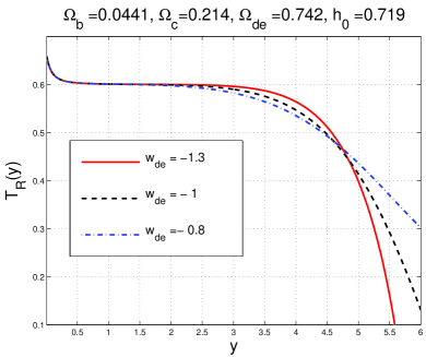
The first step of the numerical analysis is to compute $T_{\mathcal{R}}(\tau)$ and $T_{\mathrm{B}}(\tau)$ when the parameters are given exactly by Eq. (5.1) but the barotropic index of the dark energy assumes arbitrary values which can differ from the $\Lambda$CDM choice (i.e. $w_{\mathrm{de}}=-1$). The functions $T_{\mathcal{R}}(\tau)$ and $T_{\mathrm{B}}(\tau)$ have been introduced in Eq. (3.25) and control the two relevant large-scale contributions to the ISW effect. According to Eqs. (3.26) and (3.27), $T_{\mathcal{R}}(\tau)$ and $T_{\mathrm{B}}(\tau)$ can be assessed once the (numerical) evolution of the background geometry has been obtained. Such a technique is rather useful for the analytic estimate of the asymptotic limits and it otherwise demands the full (numerical) solution of the background geometry; the results of Figs. 1 and 2 $T_{\mathcal{R}}(\tau)$ and $T_{\mathrm{B}}(\tau)$ are obtained by direct numerical integration. It has been explicitly verified that, indeed, Eqs. (3.26) and (3.27) are in excellent agreement with the numeric result once the full numerical expression of the scale factor is known.

Figure 1: The evolutions of the scale factor and of $T_{{\mathcal{R}}}(y)$ are illustrated for different values of the barotropic index of dark energy $w_{\mathrm{de}}$.

In Fig. 1 (plot at the left) on the vertical axis the common logarithm of the scale factor is illustrated while on the horizontal axis the convenient time variable is given by $y=3.33\times 10^{-4}(\tau/\mathrm{Mpc})$ where $\tau$, as usual, is the conformal time coordinate. Using $y$ as integration variable, Eq. (2.1) and the related initial conditions become very simple

$$\frac{da}{dy} = \sqrt{\omega_{\mathrm{R}}+\omega_{\mathrm{M}}a+\omega_{\mathrm{de}}a^{1-3w_{\mathrm{de}}}},$$ (5.2)

$$a(y_{\mathrm{i}}) = \frac{\omega_{\mathrm{M}}}{4}y_{\mathrm{i}}^{2}+\sqrt{\omega_{\mathrm{R}}}y_{\mathrm{i}},$$ (5.3)

where $\omega_{\mathrm{R}}=h_{0}^{2}(\Omega_{\gamma}+\Omega_{\nu})$, $\omega_{\mathrm{M}}=h_{0}^{2}(\Omega_{\mathrm{b}}+\Omega_{\mathrm{c}})$ and $\omega_{\mathrm{de}}=h_{0}^{2}\Omega_{\mathrm{de}}$. The physical range of the parameters and the present normalization of the scale factor imply that $a_{0}=1$. To illustrate the trends induced by different values of $w_{\mathrm{de}}$ it is useful to plot the quantities of Fig. 1 also a bit outside their physical range (i.e. for $a>a_{0}$). The initial condition of Eq. (5.3) are imposed by making use of an exact solution of Eq. (5.2) (as well as of the other Friedmann-Lemaître equations (2.1)) in the limit $\rho_{\mathrm{de}}\to 0$. The form of the initial conditions of Eq. (5.3) implies that $y_{\mathrm{i}}$ is well before matter-radiation equality.

Always in Fig. 1 (plot at the right) the profile of $T_{{\mathcal{R}}}(y)$ is illustrated. As expected, around $y_{\mathrm{i}}$ (i.e. deep in the radiation dominated epoch) $T_{{\mathcal{R}}}(y_{\mathrm{i}})=2/3$. Then, as $y$ increases, $T_{\mathcal{R}}(y)$ reaches a flat plateau for intermediate times around decoupling where $T_{{\mathcal{R}}}(y)\simeq 3/5$ (see Fig. 1, plot at the right). Absent any late dominance of dark energy, $T_{{\mathcal{R}}}(y)\to 3/5$ exactly. The (late) deviation from the CDM asymptote (i.e. $3/5$) depends upon the specific value of $w_{\mathrm{de}}$ and determines the ISW contribution.

Figure 2: In the plots at the left and at the right the evolution of $T_{\mathrm{B}}(y)$ is illustrated, respectively, on a linear and on a logarithmic time scale. The case labeled with $w_{\mathrm{de}}=-1$ corresponds to the best fit of the WMAP 5yr data alone in the light of the $\Lambda$CDM scenario.

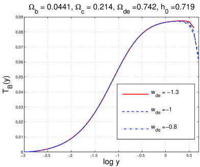
In Fig. 2 the function $T_{\mathrm{B}}(y)$ is illustrated both on a linear time scale (plot at the left) and using a logarithmic time scale (plot at the right) which better represents the early evolution before matter radiation equality and across decoupling. The arrow appearing in the left plot of Fig. 2 marks, approximately, the present time, i.e. when $a(y_{0})\simeq a_{0}=1$. In short the shape of $T_{\mathrm{B}}(y)$ can be understood as follows:

• unlike the case of $T_{\mathcal{R}}(y)$ (which reaches a constant asymptote deep in the radiation-dominated epoch, i.e. for $y\ll 1$), $T_{\mathrm{B}}(y)\to 0$ in the limit $y\to 0$;

• in the CDM paradigm $T_{\mathrm{B}}(y)$ would reach the asymptotic value $3R_{\gamma}/20\simeq 0.089$;

• both in the $\Lambda$CDM and in the wCDM cases the would be asymptotes turn into an intermediate plateau (see Fig. 2, in particular plot at the right);

• the intermediate plateau is accurately estimated by $3R_{\gamma}/20$ while the presence of a dark energy background is responsible for the deviation of $T_{\mathrm{B}}(y)$ from the CDM asymptote.

The vanishing of $T_{\mathrm{B}}(y)$ for $y\to 0$ is a consequence of the evolution of ${\mathcal{R}}(k,y)$ and, in particular, of Eqs. (2.40) and (2.41). The same observation implies that whenever ${\mathcal{R}}_{*}(k)\to 0$, ${\mathcal{R}}(k,y)\to 0$ for $y\to 0$: such an occurrence is verified (and illustrated) in the left plot of Fig. 3 where ${\mathcal{R}}(k,y)$ is shown to vanish in the limit ${\mathcal{R}}_{*}(k)\to 0$.

Figure 3: The evolution of ${\mathcal{R}}(k,y)$ in the case ${\mathcal{R}}_{*}(k)\to 0$ (plot at the left). The evolution of $\psi(k,y)/{\mathcal{R}}_{*}(k)$ for different values of the magnetic energy density.

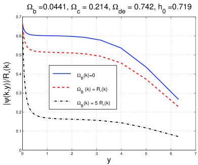
It can be speculated that the the contribution coming from $\Omega_{\mathrm{B}}(k)$ and ${\mathcal{R}}_{*}(k)$ might interfere destructively leading to an overall suppression of the large-scale contribution and, in particular, of the quadrupole. In Fig. 3 (plot at the right) this possibility seems excluded unless $\Omega_{\mathrm{B}}(k)\simeq{\mathcal{R}}_{*}(k)$. But such an extreme value would jeopardize the agreement of the theory with the acoustic region.

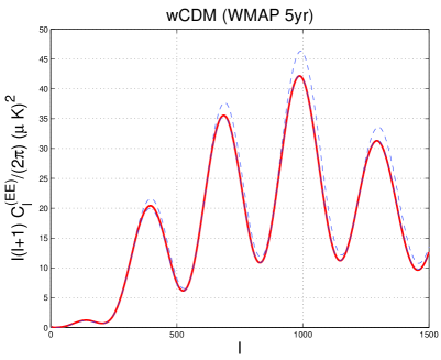
To scrutinize this point in a model-independent perspective, consider the condition $\Omega_{\mathrm{B}}(k)\simeq{\mathcal{R}}_{*}(k)$ in loose terms and postulate that the amplitude of curvature perturbations matches approximately the amplitude of the power spectrum of the magnetic energy density. Neglecting, for simplicity, the dependence upon the spectral indices we get a typical amplitude for the comoving amplitude of the magnetic field intensity which is of the order of $B_{\mathrm{L}}\simeq 22.68\,\mathrm{nG}$ where it has been assumed that ${\mathcal{A}}_{{\mathcal{R}}}=2.4\times 10^{-9}$, $k_{\mathrm{L}}=1/\mathrm{Mpc}$ and $k_{\mathrm{p}}=0.002\,\mathrm{Mpc}^{-1}$. The putative value of about $23$ nG is indeed quite large and it would totally disrupt the structure of the acoustic oscillations. This aspect can be appreciated from Fig. 4 where a magnetic field of $10$ nG already jeopardizes the observed features of the temperature autocorrelations .

In the minimal scenario [16, 52], the parameter space of the magnetized CMB anisotropies can be described in terms of the magnetic spectral index $n_{\mathrm{B}}$ and the regularized magnetic field amplitude $B_{\mathrm{L}}$. These two quantities and their relations with $\Omega_{\mathrm{B}}$ and $\sigma_{\mathrm{B}}$ (introduced in section 2) have been thoroughly discussed in previous papers [16, 17, 18]. The basic advantages of such a parametrization have been illustrated at the end of section 3 (see, in particular, Eq. (3.37) and Eq. (3.36) for the analog conventions employed in the definition of the power spectra of curvature perturbations).

Figure 4: The angular power spectra of the CMB observables in the light of the wCDM scenario when large-scale magnetic fields are included. In all the plots the barotropic index of the (fluctuating) dark energy background has been fixed to $w_{\mathrm{de}}=-0.6$.

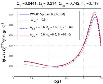
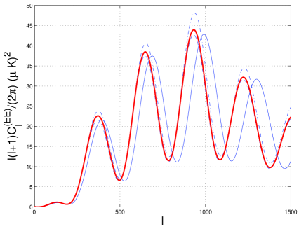
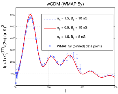
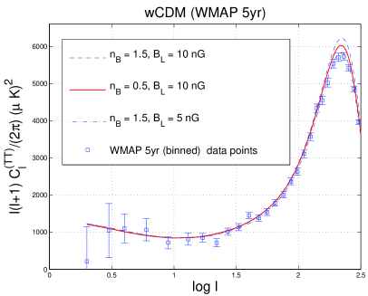
In Fig. 4 the parameters are fixed to the best fit of the WMAP 5yr data alone in the light of the $\Lambda$CDM paradigm (corresponding to $w_{\mathrm{de}}=-1$). Always in Fig. 4 the barotropic index of the dark energy is increased from $-1$ to $-0.6$ while the magnetized background is switched on. The magnetic field intensity has been chosen to be rather large (i.e. ${\mathcal{O}}(10\,\mathrm{nG})$). Examples of blue (i.e. $n_{\mathrm{B}}=1.5$) and red (i.e. $n_{\mathrm{B}}=0.5$) spectral indices are illustrated. From the TT correlations in semilogarithmic coordinates (top-right plot) as well as from the TE and EE correlations the general interplay of the dark energy and magnetized backgrounds is more clear and can be summarized as follows:

• in the large-scale domain (i.e. $\ell<50$) both the dark energy and the magnetized contribution augment the power in the TT angular power spectra;

• possible interference effects leading to an overall suppression of the lower multipoles are excluded if the acoustic oscillations are to be reproduced correctly; this statement holds in the absence of any non-adiabatic contribution (i.e. $\delta p_{\mathrm{nad}}=0$ in Eq. (2.40)) but it might change if $\delta p_{\mathrm{nad}}\neq 0$;

• the interplay between the magnetized and the dark energy backgrounds leads to a combined distortion of the peaks in the TT, TE and EE angular power spectra; since the level of distortion increases with the multipole the higher peaks look also shifted in comparison with the patterns exhibited by the underlying $\Lambda$CDM model with the same parameters and in the absence of any magnetic field.

The value $w_{\mathrm{de}}=-0.6$ chosen in Fig. 4 is rather extreme insofar as it is excluded by current fits to the WMAP 5yr data (either alone or in combination with other data sets). It is however useful highlight some general trend induced by the dark energy fluctuations.

Figures 1, 2 and 3 do also contain examples where $w_{\mathrm{de}}<-1$. When analyzing the cosmological data sets in the light of a fluctuating dark energy background it can happen that the central value of the barotropic index maximizing the likelihood for a specific data set gets smaller than $-1$. In the latter case future singularities are expected (see for instance [49]). In what follows the cases $w_{\mathrm{de}}<-1$ will be considered for completeness. Indeed the central values of the barotropic index is still debatable and does depend upon the data sets which are combined in the analysis. For the purposes of the present paper, the situation is summarized in three forthcoming paragraphs.

By analyzing the WMAP 5yr data alone in the light of the $w$CDM model we do get $w_{\mathrm{de}}=-1.06_{-0.42}^{0.41}$ while the remaining parameters are determined to be

$$(\Omega_{\mathrm{b}},\,\Omega_{\mathrm{c}},\Omega_{\mathrm{de}},\,h_{0},\,n_{\mathrm{s}},\,\epsilon_{\mathrm{re}})\equiv$$

$$(0.046^{0.018}_{-0.018},0.221_{-0.082}^{0.087},0.733^{0.10}_{-0.11},0.74^{0.15}_{-0.14},0.963^{0.016}_{-0.016},0.086^{0.017}_{-0.016});$$ (5.4)

in the case of the parameters of Eq. (5.4) the corresponding value of the normalization of the curvature perturbations is still ${\mathcal{A}}_{{\mathcal{R}}}=2.41\times 10^{-9}$ at the pivot scale of $k_{\mathrm{p}}=0.002\,\mathrm{Mpc}^{-1}$; the value of ${\mathcal{A}}_{{\mathcal{R}}}$ does not change in comparison with the corresponding value determined in connection with the parameters of Eq. (5.1).

By combining the WMAP 5yr data with the data stemming from the analysis of the baryon acoustic oscillations (BAO in what follows) [56, 57, 58] the preferred range of values of $w_{\mathrm{de}}$ becomes $-1.15_{-0.22}^{0.21}$; the remaining parameters turn out to be [3, 4, 5]:

$$(\Omega_{\mathrm{b}},\,\Omega_{\mathrm{c}},\Omega_{\mathrm{de}},\,h_{0},\,n_{\mathrm{s}},\,\epsilon_{\mathrm{re}})\equiv$$

$$(0.0419^{0.0055}_{-0.0056},0.213^{0.021}_{-0.021},\,0.745^{0.026}_{-0.026},0.739^{0.047}_{-0.048},0.958_{-0.015}^{0.015},\,0.083^{0.016}_{-0.016});$$ (5.5)

the value of ${\mathcal{A}}_{{\mathcal{R}}}$ determined in connection with the data of Eq. (5.5) increases in comparison with the corresponding values holding in the case of Eqs. (5.1) and (5.4) and it is given by ${\mathcal{A}}_{{\mathcal{R}}}=2.48\times 10^{-9}$.

Finally, by combining the WMAP 5yr data with the BAO and with all the supernovae [59, 60, 61] the central value of $w_{\mathrm{de}}$ maximizing the likelihood gets above $-1$ and it is $w_{\mathrm{de}}=-0.972_{-0.060}^{0.061}$; the remaining parameters are given, in this case, by [3, 4, 5]

$$(\Omega_{\mathrm{b}},\,\Omega_{\mathrm{c}},\Omega_{\mathrm{de}},\,h_{0},\,n_{\mathrm{s}},\,\epsilon_{\mathrm{re}})\equiv$$

$$(0.0467_{-0.0018}^{0.0018},0.231_{-0.014}^{0.014},0.722_{-0.015}^{0.015},0.697_{-0.014}^{0.014},0.962_{-0.014}^{0.014},0.085_{-0.016}^{0.016});$$ (5.6)

again the value of ${\mathcal{A}}_{{\mathcal{R}}}$ determined in connection with the data of Eq. (5.5) diminishes in comparison with the corresponding values holding in the case of Eqs. (5.5) and it is ${\mathcal{A}}_{{\mathcal{R}}}=2.43\times 10^{-9}$.

The data reported in Eqs. (5.4), (5.5) and (5.6) will be referred to as, respectively, WMAP 5yr alone, WMAP 5yr + bao, and WMAP 5yr + bao + snall. Bearing in mind the latter shorthand notations it is now appropriate to scrutinize how the simultaneous presence of large-scale magnetic fields and of the dark energy fluctuations affects the temperature and the polarization observables. This aspect is illustrated in three of the forthcoming figures, i.e. in Figs. 5, 6 and 7 where the magnetized background is studied together with the dark energy background for the reference models discussed in Eqs. (5.4), (5.5) and (5.6).

Figure 5: Large-scale magnetic fields are included together with dark energy fluctuations in the case of the wCDM scenario (see Eq. (5.4) for the list of the parameters). In the TT and TE angular power spectra the binned points of the WMAP 5yr data are also reported. In all plots the fluctuating dark energy contribution has been included and, consistently with Eq. (5.4), $w_{\mathrm{de}}=-1.06$.

In Fig. 5 the parameters of the wCDM model have been chosen as in Eq. (5.4) with $w_{\mathrm{de}}=-1.06$ corresponding to the best fit in the light of the WMAP 5yr data points. It is superficially clear that the string of parameters of Eq. (5.1) does not differ, qualitatively, from the ones of Eq. (5.4). As expected, the inclusion of the magnetized contribution distorts the higher peaks. Three representative values of the parameter space of the magnetized wCDM scenario are illustrated:

• (i) the curves with $n_{\mathrm{B}}=1.5$ and $B_{\mathrm{L}}=10$ nG are representative of the region with high magnetic field intensity and blue spectral index (i.e. $n_{\mathrm{B}}>1$);

• (ii) the curves with $n_{\mathrm{B}}=0.5$ and $B_{\mathrm{L}}=10$ nG are representative of the region with high magnetic field intensity and red spectral index (i.e. $n_{\mathrm{B}}<1$);

• (iii) the curves with $n_{\mathrm{B}}=1.5$ and $B_{\mathrm{L}}=5$ nG are representative of the region with intermediate magnetic field intensities and blue spectral index.

The regions of the parameter space corresponding to $(i)$ and $(ii)$ are roughly incompatible with the observed angular power spectra as it can be easily argued by superimposing the curves to the binned data of the TT and TE correlations [3, 4, 5]. Furthermore, the values of the parameters of regions $(i)$ and $(ii)$ lie in a portion of the parameter space which has been excluded by estimating the parameters of the magnetized background in the light of the magnetized extension of the standard $\Lambda$CDM scenario. Does the inclusion of a fluctuating dark energy background make the difference? The answer to this question will be the subject of the remaining considerations of this section. Notice also that the choice of the parameters corresponding to $(iii)$ seems to be qualitatively compatible with the observations. One of the purposes of the following discussion will be to make such a statement more quantitative.

As a last remark concerning Fig. 5, the value of the barotropic index of dark energy (i.e. $w_{\mathrm{de}}=-1.06$) is rather close to the $\Lambda$CDM determination and this occurrence excludes interference effects such as the ones observed in Fig. 4 where $w_{\mathrm{de}}$ differs from $-1$ appreciably (i.e. $w_{\mathrm{de}}=-0.6$).

Figure 6: Large-scale magnetic fields are included for the wCDM best fit when the WMAP 5yr data are combined with the ones stemming from the baryon acoustic oscillations. As in Fig. 5 the fluctuations in the dark energy background have been taken into account; $w_{{\mathrm{de}}}=-1.15$ (as it must be from Eq. (5.5)).

Figure 7: Large-scale magnetic fields are included for the wCDM best fit when the WMAP 5yr data are combined with the baryon acoustic oscillations and with all supernova data. As in Figs. 5 and 6 the fluctuations in the dark energy background have been taken into account; $w_{{\mathrm{de}}}=-0.972$ (in agreement with Eq. (5.6))

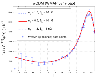
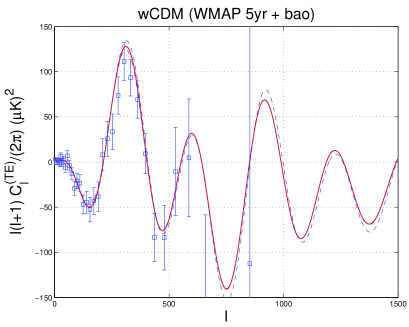
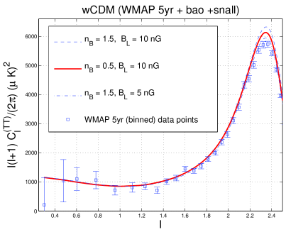
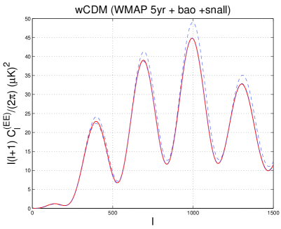
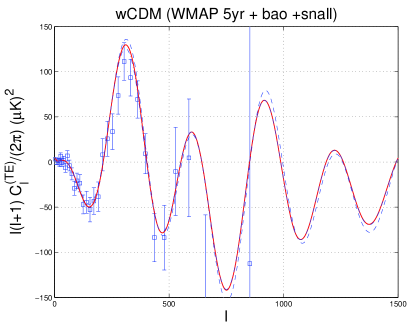
In Fig. 6 and 7 the dark energy background and the other wCDM parameters are fixed, respectively, as in Eqs. (5.5) and (5.6). The considerations suggested by Fig. 4 are confirmed, in some sense, also by Figs. 5 and 6. Extreme values of the magnetic field intensity ${\mathcal{O}}(10\,\mathrm{nG})$ are incompatible with the observations both in the case of red and blue spectral indices.

The joined two-dimensional marginalized contours for the various cosmological parameters identified already by the analyses of the WMAP 3yr data are ellipses with an approximate Gaussian dependence on the confidence level as they must be in the Gaussian approximation (see, e. g. [1]). The parameter space of the magnetized CMB anisotropies can then be scanned in the presence of dark energy fluctuations by using the same technique discussed in [16, 17] and applied to the case of the $\Lambda$CDM paradigm.

Figure 8: Likelihood contours in the plane $(n_{\mathrm{B}},\,B_{\mathrm{L}})$. In both plots the inner curve corresponds to $\Delta\chi^{2}=2.3$ (i.e. $68.3$% or $1\,\sigma$ of likelihood content) while the outer curve corresponds to $\Delta\chi^{2}=6.17$ (i.e. $95.4\,$% or $2\,\sigma$ of likelihood content).

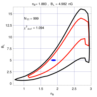
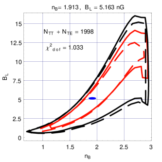
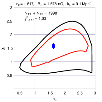
In Fig. 8 the filled (ellipsoidal) spots in both plots mark the minimal value of the $\chi^{2}$ (i.e. $\chi^{2}_{\mathrm{min}}$) obtained in the context of the WMAP 5yr data alone (see, e.g., Eq (5.4)); the closed curves represent the likelihood contours in the two parameters $n_{\mathrm{B}}$ and $B_{\mathrm{L}}$. In both plots of Fig. 8 the boundaries of the two regions contain $68.3\,$% and $95.4\,$% of likelihood as the values for which the $\chi^{2}$ has increased, respectively, by an amount $\Delta\chi^{2}=2.3$ and $\Delta\chi^{2}=6.17$. In the plot at the left of Fig. 1 the data points used for the analysis correspond to the measured TT correlations contemplating $N_{\mathrm{TT}}=999$ experimental points from $\ell=2$ to $\ell=100$. In the plot at the right the data points include, both, the TT and TE correlations and the total number of data points increases to $N_{\mathrm{TT}}+N_{\mathrm{TE}}=1998$. The values of $n_{\mathrm{B}}$ and $B_{\mathrm{L}}$ minimizing the $\chi^{2}$ when only the TT correlations are considered turn out to be $n_{\mathrm{B}}=1.883$ and $B_{\mathrm{L}}=4.982\,\mathrm{nG}$; in this case the reduced $\chi^{2}$ is $1.094$. When also the TE correlations are included in the analysis the reduced $\chi^{2}$, i.e. $\chi^{2}_{\mathrm{dof}}$, diminishes from $1.094$ to $1.033$ and the values of $n_{\mathrm{B}}$ and $B_{\mathrm{L}}$ minimizing the $\chi^{2}$ become $n_{\mathrm{B}}=1.913$ and $B_{\mathrm{L}}=5.163\,\mathrm{nG}$. The points of the parameter leading to $\chi^{2}_{\mathrm{min}}$ maximize the likelihood in the Gaussian approximation (see [16] and [17]).

In a frequentist approach, the boundaries of the confidence regions represent exclusion plots at $68.3\,$% and $95.4\,$% confidence level. In Fig. 8 (plot at the right) the inner dashed curve corresponds to the $68.3\,$% boundary while the outer dashed line corresponds to the $95.4\,$% boundary as determined in the context of the magnetized $\Lambda$CDM scenario and with the very same set of data [16]. By comparing the dashed and full contour plots in Fig. 8 (right plot) the shapes of the excluded regions are compatible in the two cases. The overlap seems even to increase by increasing the confidence range. At the same time the addition of a fluctuating dark energy background pins down systematically larger values of the magnetic field parameters. More specifically, by looking at the parameters corresponding to $\chi^{2}_{\mathrm{min}}$, we can say that

$$(n_{\mathrm{B}},B_{\mathrm{L}})_{\Lambda\mathrm{CDM}}=(1.598,\,3.156\mathrm{nG})\to(n_{\mathrm{B}},B_{\mathrm{L}})_{\mathrm{{\it w}CDM}}=(1.883,\,4.982\,\mathrm{nG}),$$ (5.7)

$$(n_{\mathrm{B}},B_{\mathrm{L}})_{\Lambda\mathrm{CDM}}=(1.616,\,3.218\mathrm{nG})\to(n_{\mathrm{B}},B_{\mathrm{L}})_{\mathrm{{\it w}CDM}}=(1.913,\,5.163\,\mathrm{nG}),$$ (5.8)

where Eq. (5.7) corresponds to $N_{\mathrm{TT}}=999$ (i.e. only the unbinned points of the TT correlations are used) while Eq. (5.8) does correspond to $N_{\mathrm{TT}}+N_{\mathrm{TE}}=1998$ (i.e. the unbinned points of the TT and TE correlations are used).

Equations (5.7) and (5.8) show that the magnetic field parameters minimizing the $\chi^{2}$ (and maximizing the likelihood) do (slightly) increase when the dark energy component is allowed to fluctuate. Of course the slight numerical difference does not change the physical conclusions obtained in the context of the magnetized $\Lambda$CDM class of models: the preferred region is for blue spectral indices and moderate magnetic field intensities.

Figure 9: Same quantities as in Fig. 8 but in the case when wCDM scenario is analyzed in the light of the WMAP 5yr +bao data (see Eq. (5.5)).

In Fig. 9 the likelihood contours are obtained when the best fit parameters are determined from the wCDM parameters arising when the WMAP 5yr data are combined with the data stemming from the baryon acoustic oscillations (see Eq. (5.5)). In this case, again, the shapes of the likelihood contours are qualitatively a bit different but quantitatively compatible with the cases of Fig. 8 and of Eq. 9.

Figure 10: The effect of change in the magnetic pivot scale $k_{\mathrm{L}}$ is illustrated in the case of the WMAP 5yr data alone in the $\Lambda$CDM case (left plot) and in the wCDM case (plot at the right).

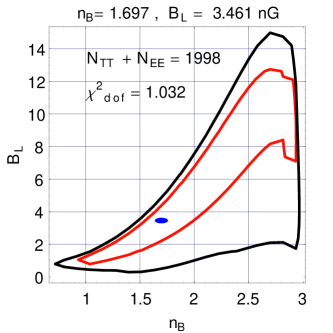
As expected a decrease of $k_{\mathrm{L}}$ lowers the value of the regularized magnetic field intensity $B_{\mathrm{L}}$. This effect is illustrated in Fig. 10. In the right plot, the likelihood contours are computed when $k_{\mathrm{L}}=0.1\,\mathrm{Mpc}^{-1}$; the parameters of the $w$CDM paradigm are determined from Eq. (5.4). In the plot at the left the same analysis is performed for the $\Lambda$CDM case when, again, the other parameters are determined from the WMAP 5yr data alone. The exclusion plots of Figs. 8, 9 and 10 explain, a posteriori, why in the plots of Fig. 5, 6 and 7 the minimal amount of distortions was provided by the dot-dashed curves. The dot-dashed curves corresponded, in those figures, to the region $(iii)$ i.e. the region where the moderate magnetic field intensities corresponded to blue magnetic spectral indices.

6 Concluding remarks

The analysis of magnetized CMB anisotropies has been extended, for the first time, to the case when the dark energy background fluctuates. This class of models, conventionally labeled as magnetized $w$CDM, generalizes the magnetized $\Lambda$CDM scenario. The ordinary and integrated Sachs-Wolfe effects have been analyzed in the light of the $w$CDM paradigm. In the minimal realization of the scenario (i.e. in the absence of non-adiabatic components in the initial conditions) the contribution of the magnetized background is not sufficient to compensate the effect induced on the adiabatic mode by the late-time dynamics of the dark energy background. Possible compensating effects arise for excessively large values of the magnetic field intensity; these values are already constrained by the structure of the acoustic oscillations.

Since the modified initial conditions of the Einstein-Boltzmann hierarchy allow for the simultaneous presence of dark energy perturbations and of large-scale magnetic fields, the morphology of the distortions arising in the magnetized $w$CDM scenario has been compared with what happens when the dark energy background is not dynamical. The modifications induced by the fluctuating dark energy component on the shapes of the $1$- and $2$-$\sigma$ contours in the parameter space of the magnetized background have been computed. At $95$ % confidence level, the allowed spectral indices and magnetic field intensities turn out to be systematically larger than those determined in the framework of the magnetized $\Lambda$CDM paradigm.

Appendix A Synchronous frame

It is understood that all the quantities appearing in this section of the appendix are evaluated in the synchronous frame. The evolution equation of the intensity brightness perturbations are given by

$$\Delta_{\mathrm{I}}^{\prime}+(ik\mu+\epsilon^{\prime})\Delta_{\mathrm{I}}=-\xi^{\prime}-\frac{\mu^{2}}{2}(h+6\xi)^{\prime}+\epsilon^{\prime}\biggl{[}\Delta_{\mathrm{I}0}+\mu v_{\mathrm{b}}+\frac{(1-3\mu^{2})S_{\mathrm{P}}(k,\tau)}{4}\biggr{]},$$ (A.1)

$$v_{\mathrm{b}}^{\prime}+{\mathcal{H}}v_{\mathrm{b}}+\frac{\epsilon^{\prime}}{R_{\mathrm{b}}}(3i\Delta_{\mathrm{I}1}+v_{\mathrm{b}})+ik\frac{\Omega_{\mathrm{B}}-4\sigma_{\mathrm{B}}}{4R_{\mathrm{b}}}.$$ (A.2)

The formal solution of Eq. (A.1) can be written, after integrating once by parts, as:

$$\Delta_{\mathrm{I}}(k,\mu,\tau_{0})=\int_{0}^{\tau_{0}}\,e^{-\epsilon(\tau,\tau_{0})}\biggl{[}-\xi^{\prime}-\frac{(h+6\xi)^{\prime\prime\prime}}{2k^{2}}\biggr{]}e^{-i\mu x(\tau)}\,d\tau$$ (A.3)

$$+ \int_{0}^{\tau_{0}}{\mathcal{K}}(\tau)e^{-i\mu x(\tau)}\biggl{[}\Delta_{\mathrm{I}0}-\frac{(h+6\xi)^{\prime\prime}}{2k^{2}}+\mu v_{\mathrm{b}}+\frac{i\mu}{2k}(h+6\xi)^{\prime}+\frac{(1-3\mu^{2})S_{\mathrm{P}}(k,\tau)}{4}\biggr{]},$$

where, as in the bulk of the paper, $x(\tau)=k(\tau_{0}\tau)$. The visibility function is defined in terms of the optical depth are defined as in Eq. (3.3). The integration by parts can be further used in Eq. (A.1):

$$\Delta_{\mathrm{I}}(k,\mu,\tau_{0}) = \int_{0}^{\tau_{0}}\frac{e^{-i\mu x(\tau)}}{4k^{2}}\tilde{S}_{\mathrm{P}}(k,\tau_{0}),$$ (A.4)

$$\tilde{S}_{\mathrm{P}}(k,\tau_{0}) = {\mathcal{K}}(\tau)[4k^{2}\Delta_{\mathrm{I}0}-(h+6\xi)^{\prime\prime}+4ikv_{\mathrm{b}}^{\prime}+k^{2}S_{\mathrm{P}}+3S_{\mathrm{P}}^{\prime\prime}]$$ (A.5)

$$+ {\mathcal{K}}^{\prime}[6S_{\mathrm{P}}^{\prime}+4ikv_{\mathrm{b}}-2(h+6\xi)^{\prime}]+3S_{\mathrm{P}}{\mathcal{K}}^{\prime\prime}$$

$$-e^{-\epsilon(\tau,\tau_{0})}[4k^{2}\xi^{\prime}+2(h+6\xi)^{\prime}],$$

but in spite of the simplifications obtained in Eqs. (A.4) and (A.5), Eq. (A.3) is still the most direct for separating the ordinary and the integrated Sachs-Wolfe contribution in the presence of a sudden drop in the opacity at $\tau_{\mathrm{rec}}$. In this case Eqs. (A.3) implies

$$\Delta_{\mathrm{I}}(k,\mu,\tau_{0})=\Delta^{(\mathrm{SW})}_{\mathrm{I}}(k,\mu,\tau_{0})+\Delta^{(\mathrm{ISW})}_{\mathrm{I}}(k,\mu,\tau_{0}),$$ (A.6)

$$\Delta^{(\mathrm{ISW})}_{\mathrm{I}}(k,\mu,\tau_{0})=\int_{\tau_{\mathrm{rec}}}^{\tau_{0}}\biggl{[}-\xi^{\prime}-\frac{(h+6\xi)^{\prime\prime\prime}}{2k^{2}}\biggr{]}e^{-i\mu x(\tau)}\,d\tau,$$ (A.7)

$$\Delta^{(\mathrm{SW})}_{\mathrm{I}}(k,\mu,\tau_{0})=\biggl{[}\Delta_{\mathrm{I}0}-\frac{(h+6\xi)^{\prime\prime}}{2k^{2}}\biggr{]}_{\tau_{\mathrm{rec}}}e^{-i\mu y_{\mathrm{rec}}}.$$ (A.8)

Recalling that, by definition, $y_{\mathrm{rec}}=x(\tau_{\mathrm{rec}})=k(\tau_{0}-\tau_{\mathrm{rec}})$ the SW contribution can be easily rearranged as

$$\Delta^{(\mathrm{SW})}_{\mathrm{I}}(k,\mu,\tau_{0})=\biggl{[}\Delta_{\mathrm{I}0}(k,\tau)-\xi(k,\tau)+{\mathcal{H}}\frac{(h+6\xi)^{\prime}}{k^{2}}\biggr{]}_{\tau_{\mathrm{rec}}}e^{-i\mu y_{\mathrm{rec}}},$$ (A.9)

where the evolution equation

$$(h+6\xi)^{\prime\prime}+2{\mathcal{H}}(h+6\xi)^{\prime}=2k^{2}\xi+{\mathcal{O}}(k^{2}\tau^{2})$$ (A.10)

has been used explicitly. In Eq. (A.10) the various anisotropic stresses have been neglected; Eq. (A.10) is the synchronous version of Eq. (2.20), as it can be easily verified by using the procedure swiftly illustrated in section 1. Recalling that $\Delta_{\mathrm{I}0}=4\delta_{\gamma}$, the solution of synchronous gauge version of Eq. (2.27) implies

$$\Delta_{\mathrm{I}0}=-\frac{R_{\gamma}\Omega_{\mathrm{B}}}{4}+\frac{h}{6}+{\mathcal{O}}(k^{2}\tau^{2}).$$ (A.11)

To obtain the explicit form of Eq. (A.9) we need the evolution of $\xi(k,\tau)$ and $h(k,\tau)$ across equality. By using Eq. (2.8) and (2.38) we obtain

$$\xi(k,\tau)={\mathcal{R}}_{*}(k)-\frac{R_{\gamma}\Omega_{\mathrm{B}}(k)}{8}{\mathcal{G}}_{1}(\alpha),$$ (A.12)

$$h(k,\tau)=\frac{3}{4}R_{\gamma}\Omega_{\mathrm{B}}(k){\mathcal{G}}_{1}(\alpha)+k^{2}\tau_{1}^{2}{\mathcal{R}}_{*}(k){\mathcal{G}}_{2}(\alpha)-\frac{3}{4}R_{\gamma}\Omega_{\mathrm{B}}(k)k^{2}\tau_{1}^{2}{\mathcal{G}}_{3}(\alpha),$$ (A.13)

$$\frac{(h+6\xi)^{\prime}}{2k^{2}}=\frac{{\mathcal{R}}_{*}(k)}{15}{\mathcal{G}}_{4}(\alpha)+\frac{R_{\gamma}\Omega_{\mathrm{B}}}{20}{\mathcal{G}}_{5}(\alpha),$$ (A.14)

where $\alpha=a/a_{\mathrm{eq}}=[(\tau/\tau_{1})^{2}+2(\tau/\tau_{1})]$ solves Eq. (2.1) across equality and where the five functions ${\mathcal{G}}_{i}(\alpha)$ are given by:

$${\mathcal{G}}_{1}(\alpha)=2\frac{[\alpha(\alpha-4)+8(\sqrt{\alpha+1}-1)]}{\alpha^{2}},$$ (A.15)

$${\mathcal{G}}_{2}(\alpha)=\frac{[\alpha^{3}-2\alpha^{2}+8\alpha+16(1-\sqrt{\alpha+1})]}{{5\alpha^{2}}},$$ (A.16)

$${\mathcal{G}}_{3}(\alpha)=\frac{\{32(\sqrt{\alpha+1}-1)+\alpha[\alpha(3\alpha-26)-16]+60\sqrt{\alpha+1}[\alpha-\ln{(\alpha+1)]}\}}{{45\alpha^{2}}},$$ (A.17)

$${\mathcal{G}}_{4}(\alpha)=\frac{\sqrt{1+\alpha}[3\alpha^{2}-4\alpha+8]-8}{\alpha^{2}},$$ (A.18)

$${\mathcal{G}}_{5}(\alpha)=\frac{\sqrt{\alpha+1}[24-\alpha^{2}+8\alpha]-4(5\alpha+6)}{\alpha^{2}}.$$ (A.19)

Using Eqs. (A.15)–(A.19) the ordinary SW contribution can be written as

$$\Delta^{(\mathrm{SW})}_{\mathrm{I}}(k,\mu,\tau_{0})=\biggl{[}-\frac{{\mathcal{R}}_{*}(k)}{5}{\mathcal{S}}{\mathcal{W}}_{{\mathcal{R}}}(\alpha_{\mathrm{rec}})+\frac{R_{\gamma}\Omega_{\mathrm{B}}(k)}{20}\,{\mathcal{S}}{\mathcal{W}}_{\mathrm{B}}(\alpha_{\mathrm{rec}})+{\mathcal{O}}(k^{2}\tau^{2})]e^{-i\mu y_{\mathrm{rec}}}$$ (A.20)

where ${\mathcal{S}}{\mathcal{W}}_{{\mathcal{R}}}(\alpha_{\mathrm{rec}})$ and ${\mathcal{S}}{\mathcal{W}}_{\mathrm{B}}(\alpha_{\mathrm{rec}})$ are the two functions appearing, respectively, in Eqs. (3.14) and (3.15).

Appendix B Explicit derivation of $T_{\mathcal{R}}(\tau)$ and $T_{\mathrm{B}}(\tau)$

Consider Eq. (2.7) in terms of the conformally Newtonian variables. The first equality can be written, for immediate convenience, as

$${\mathcal{R}}=-\psi+\frac{H^{2}}{\dot{H}}\biggl{[}\psi+\frac{\dot{\psi}}{H}\biggr{]},\qquad\frac{\partial}{\partial t}\biggl{(}\frac{a\psi}{H}\biggr{)}=a{\mathcal{R}}\frac{\dot{H}}{H^{2}},$$ (B.1)

where we only passed from the conformal time coordinate $\tau$ to the cosmic time coordinate $t$ and we recalled that $dt\,=a(\tau)d\tau$; it is also practical to use the well known identities $\dot{H}=({\mathcal{H}}^{\prime}-{\mathcal{H}}^{2})/a^{2}$ and $H={\mathcal{H}}/a$. From Eq. (B.1) by integrating once with respect to $t$ the solution for $\psi(k,t)$ then becomes

$$\psi(k,t)=-{\mathcal{R}}(k,t)+\frac{H}{a}\int_{0}^{t}\frac{a\dot{{\mathcal{R}}}}{H}\,dt^{\prime}+\frac{H}{a}\int_{0}^{t}{\mathcal{R}}(k,t^{\prime})a(t^{\prime})\,dt^{\prime},$$ (B.2)

where we integrated by parts and used that

$$\frac{\partial}{\partial t}\biggl{(}\frac{a{\mathcal{R}}}{H}\biggr{)}=-\frac{\dot{H}}{H^{2}}a{\mathcal{R}}+\frac{\dot{a}}{H}{\mathcal{R}}+\frac{a\dot{{\mathcal{R}}}}{H}.$$ (B.3)

From Eqs. (2.39), (2.40) and (2.41), neglecting the electric and Ohmic contributions, $\dot{{\mathcal{R}}}(k,t)$ is given by:

$$\dot{{\mathcal{R}}}=-\frac{H\,\delta p_{\mathrm{nad}}}{p_{\mathrm{t}}+\rho_{\mathrm{t}}}+\biggl{(}c_{\mathrm{st}}^{2}-\frac{1}{3}\biggr{)}\frac{H\delta_{\mathrm{s}}\rho_{\mathrm{B}}}{p_{\mathrm{t}}+\rho_{\mathrm{t}}},$$ (B.4)

whose formal solution can be written as:

$${\mathcal{R}}(k,t^{\prime})={\mathcal{R}}_{*}(k)-\int_{0}^{t^{\prime}}\frac{H(t^{\prime})\delta p_{\mathrm{nad}}(k,t^{\prime})}{p_{\mathrm{t}}+\rho_{\mathrm{t}}}dt^{\prime\prime}+\int_{0}^{t^{\prime}}\frac{H(t^{\prime\prime})\delta_{\mathrm{s}}\rho_{\mathrm{B}}(k,t^{\prime\prime})}{p_{\mathrm{t}}+\rho_{\mathrm{t}}}\biggl{(}c_{\mathrm{st}}^{2}-\frac{1}{3}\biggr{)}dt^{\prime\prime}.$$ (B.5)

If we now insert Eq. (B.5) into Eq. (B.2) and go back to the conformal time coordinate we can write

$$\psi(k,\tau)=-{\mathcal{R}}_{*}(k)T_{\mathcal{R}}(\tau)+R_{\gamma}\Omega_{\mathrm{B}}(k)T_{\mathrm{B}}(\tau)$$ (B.6)

where $T_{\mathcal{R}}(\tau)$ and $T_{\mathrm{B}}(\tau)$ are given by Eqs. (3.26) and (3.27). For sake of simplicity and for comparison with other treatments consider, for instance, the case of the $\Lambda$CDM scenario where

$$a(t)=a_{1}\biggl{[}\sinh{\biggl{(}\frac{3}{2}H_{0}t\biggr{)}}\biggr{]}^{2/3}.$$ (B.7)

In the cosmic time coordinate $T_{{\mathcal{R}}}(t)$ can be written as

$$T_{{\mathcal{R}}}(t)=1-\frac{H(t)}{a(t)}\int_{0}^{t}a(t^{\prime})dt^{\prime}$$ (B.8)

It is now easy to show that, for $t\to 0$, $a(t)\simeq t^{2/3}$ and $T_{{\mathcal{R}}}(t)\simeq-(3/5)$. For $t\to\infty$ $T_{{\mathcal{R}}}(t)\simeq e^{-H_{0}t}$. Unfortunately, in the most general situation of the $w$CDM scenario, the semi-anaytic estimates are not that simple and the numerical evaluation of $T_{\mathcal{R}}(\tau)$ and $T_{\mathrm{B}}(\tau)$ is often mandatory (see, for instance, the initial part of section 5).

Appendix C Generalization of certain integral representations

In the present study there is often the need of generalizing certain integral representations of the power spectrum of the ISW and of its correlation with the SW effect. For instance, in the simplest case of adiabatic fluctuations we shall have that the autocorrelation if the ISW and its cross correlation with the SW term boils down to the following pair of expressions:

$$C_{\ell}^{(\mathrm{ISW})}=\int_{\tau_{{\mathrm{rec}}}}^{\tau_{0}}\frac{dT_{{\mathcal{R}}}}{d\tau_{1}}\,d\tau_{1}\int_{\tau_{{\mathrm{rec}}}}^{\tau_{0}}\frac{dT_{{\mathcal{R}}}}{d\tau_{2}}\,d\tau_{2}f_{\ell}(\tau_{1},\tau_{2},n_{\mathrm{s}}),$$ (C.1)

$$C_{\ell}^{(\mathrm{cross})}=\frac{1}{5}\int_{\tau_{{\mathrm{rec}}}}^{\tau_{0}}\frac{dT_{{\mathcal{R}}}}{d\tau}\,d\tau\int_{\tau_{{\mathrm{rec}}}}^{\tau_{0}}f_{\ell}(\tau,\tau_{{\mathrm{rec}}},n_{\mathrm{s}}),$$ (C.2)

where

$$f_{\ell}(a,b,n_{\mathrm{s}})=\frac{8\pi^{2}{\mathcal{A}}_{{\mathcal{R}}}\,k_{\mathrm{p}}^{1-n_{\mathrm{s}}}}{\sqrt{a\,b}}\int_{0}^{\infty}k^{n_{\mathrm{s}}-3}\,J_{\ell+1/2}(ka)\,J_{\ell+1/2}(kb).$$ (C.3)

The expressions of Eqs. (C.1) and (C.2) are just illustrative since the same problem arises in the case of the transfer functions of the magnetic component. To evaluate expressions like the ones of Eqs. (C.1) and (C.2) one might choose to perform first the (numerical) integrations over the conformal time coordinate and then the integrations over the modulus of the wavevector $k$. The idea is to reverse this order and integrate first over $k$. In doing so we are led, in general terms, to integrals like

$$\int_{0}^{\infty}k^{-\lambda}J_{\nu}(ka)J_{\nu}(kb)dk=$$

$$\frac{a^{\nu}\Gamma\biggl{(}\nu+\frac{1-\lambda}{2}\biggr{)}}{2^{\lambda}b^{\nu-\lambda+1}\Gamma\biggl{(}\frac{\lambda+1}{2}\biggr{)}\Gamma(\nu+1)}F\biggl{[}\nu+\frac{1-\lambda}{2},\frac{1-\lambda}{2};\nu+1;\frac{a^{2}}{b^{2}}\biggr{]}.$$ (C.4)

In terms of the illustrative examples of Eqs. (C.1) and (C.2), $\nu=(\ell+1/2)$ and $\lambda=3-n_{\mathrm{s}}$. Equation (C.4) can be found, for instance, in Ref. [47] (see formula 6.574, page 675).

It is more practical, for the purpose of approximate evaluations, to relate the hypergeometric functions to the associated Legendre functions. This was the strategy followed in the first attempt to evaluate analytically the ISW contribution in the $\Lambda$CDM model [8]. The latter analysis has been performed is the case of (exactly) scale-invariant contribution. In spite of the fact that the explicit dependence upon the spectral index is unimportant for orders of magnitude estimates, the habit of computing analytically the ISW contribution for the exactly scale-invariant case persists [11]. In what follows the integral representation of the two-point function for the ISW will be directly related to the associated Legendre functions but for a generic spectral index.

Consider an hypergeometric function parametrized as $F(\alpha,\,\beta;\,\gamma;\,z)$. It can be shown that if two of the numbers $(\gamma-1)$, $(\alpha-\beta)$ and $(\alpha+\beta-\gamma)$ are equal (or if one of them is equal to $1/2$) then there exist a quadratic transformation which allows to connect the hypergeometric function to a Legendre function whose argument will be suitable for (approximate) semi-analytic integrations. Indeed in the case of Eq. (C.4) $\alpha=\nu+(1-\lambda)/2$, $\beta=(1-\lambda)/2$ and $\gamma=\nu+1$; this observation implies that $(\alpha-\beta)$ and $(\gamma-1)$ are both equal to $\nu$. Consequently, the general quadratic relation [48]

$$F(\alpha,\,\beta;\,2\beta;\,z)=\biggl{[}\frac{1+\sqrt{1-z}}{2}\biggr{]}^{-2\alpha}F\biggl{[}\alpha,\,\alpha-\beta+\frac{1}{2};\,\beta+\frac{1}{2};\,\biggl{(}\frac{1-\sqrt{1-z}}{1+\sqrt{1-z}}\biggr{)}^{2}\biggr{]},$$ (C.5)

implies, in the case of Eq. (C.4)

$$F\biggl{[}\nu+\frac{1-\lambda}{2},\frac{1-\lambda}{2};\nu+1;\frac{a^{2}}{b^{2}}\biggr{]}=\biggl{(}\frac{b}{b+a}\biggr{)}^{2\nu+1-\lambda}F\biggl{[}\nu+\frac{1-\lambda}{2},\,\nu+\frac{1}{2};2\nu+1;\frac{4ab}{(a+b)^{2}}\biggr{]}.$$ (C.6)

It also follows that that

$$\int_{0}^{\infty}k^{-\lambda}J_{\nu}(ka)J_{\nu}(kb)dk=$$

$$\frac{a^{\nu}\,b^{\nu}}{2^{\lambda}(a+b)^{2\nu+1-\lambda}}\frac{\Gamma\biggl{(}\nu+\frac{1-\lambda}{2}\biggr{)}}{\Gamma\biggl{(}\frac{1+\lambda}{2}\biggr{)}\Gamma(\nu+1)}F\biggl{[}\nu+\frac{1-\lambda}{2},\,\nu+\frac{1}{2};2\nu+1;\frac{4ab}{(a+b)^{2}}\biggr{]}.$$ (C.7)

The hypergeometric function appearing in Eq. (C.7) can be further transformed according to the general relation (see [48] , p. 560)

$$F(\alpha,\,\beta;\,2\beta;\,z)=\biggl{(}1-\frac{z}{2}\biggr{)}^{-\alpha}F\biggl{[}\frac{\alpha}{2},\,\frac{\alpha+1}{2};\,\beta+\frac{1}{2};\,\frac{z^{2}}{(2-z)^{2}}\biggr{]}.$$ (C.8)

In our case Eq. (C.8) implies

$$F\biggl{[}\nu+\frac{1-\lambda}{2},\,\nu+\frac{1}{2};\,2\nu+1;\,\frac{4ab}{(a+b)^{2}}\biggr{]}=$$

$$\biggl{[}\frac{a^{2}+b^{2}}{(a+b)^{2}}\biggr{]}^{-\nu-\frac{1}{2}+\frac{\lambda}{2}}F\biggl{[}\frac{\nu}{2}+\frac{1-\lambda}{4},\,\frac{\nu}{2}-\frac{\lambda}{4}+\frac{3}{4};\nu+1;\frac{4a^{2}b^{2}}{(a^{2}+b^{2})}\biggr{]}.$$ (C.9)

Using Eq. (C.9) we also have that:

$$\int_{0}^{\infty}k^{-\lambda}\,J_{\nu}(ka)\,J_{\nu}(kb)dk=\frac{a^{\nu}\,b^{\nu}}{2^{\lambda}(a^{2}+b^{2})^{\nu+(1-\lambda)/2}}\frac{\Gamma\biggl{(}\nu+\frac{1-\lambda}{2}\biggr{)}}{\Gamma\biggl{(}\frac{\lambda+1}{2}\biggr{)}\Gamma(\nu+1)}$$ (C.10)

$$\times F\biggl{[}\frac{\nu}{2}-\frac{\lambda}{4}+\frac{3}{4},\,\frac{\nu}{2}+\frac{1-\lambda}{4};\nu+1;\frac{4a^{2}b^{2}}{(a^{2}+b^{2})^{2}}\biggr{]};$$

the hypergeometric function appearing in Eq. (C.10) can be finally related to the associated Legendre functions according to the general relation

$$F\biggl{[}1+\frac{n+m}{2},\,\frac{1}{2}+\frac{m+n}{2};\,n+\frac{3}{2};\,\frac{1}{z^{2}}\biggr{]}=$$

$$e^{-i\,m\pi}\frac{z^{m+n+1}}{(z^{2}-1)^{m/2}}\frac{2^{n+1}}{\sqrt{\pi}}\frac{\Gamma\biggl{(}n+\frac{3}{2}\biggr{)}}{\Gamma(m+n+1)}Q_{n}^{m}(z),$$ (C.11)

where $Q_{n}^{m}(z)$ are the associated Legendre functions of second order. Matching Eq. (C.11) with the expression appearing in Eq. (C.10) we shall have

$$F\biggl{[}\frac{\nu}{2}-\frac{\lambda}{4}+\frac{3}{4},\,\frac{\nu}{2}+\frac{1-\lambda}{4};\nu+1;\frac{4a^{2}b^{2}}{(a^{2}+b^{2})^{2}}\biggr{]}=$$

$$\biggl{(}\frac{a^{2}+b^{2}}{2ab}\biggr{)}^{\nu+1/2}\biggl{(}\frac{a^{2}-b^{2}}{a^{2}+b^{2}}\biggr{)}^{\lambda/2}\frac{\Gamma(\nu+1)}{\Gamma\biggl{(}\nu+\frac{1+\lambda}{2}\biggr{)}}\frac{2^{\nu+1/2}}{\sqrt{\pi}}e^{-i\pi\lambda/2}Q_{\nu-1/2}^{\lambda/2}\biggl{(}\frac{a^{2}+b^{2}}{2ab}\biggr{)}.$$ (C.12)

where we used the fact that

$$Q_{n}^{-m}(y)=e^{-2i\pi m}\frac{\Gamma(n-m+1)}{\Gamma(n+m+1)}Q_{n}^{m}(y).$$ (C.13)

Thus, in conclusion, we shall have that

$$\int_{0}^{\infty}k^{-\lambda}J_{\nu}(ka)J_{\nu}(kb)dk=$$

$$\frac{(a^{2}-b^{2})^{\lambda/2}}{2^{\lambda}\sqrt{ab}}\frac{\Gamma\biggl{(}\nu+\frac{1-\lambda}{2}\biggr{)}}{\Gamma\biggl{(}\frac{1+\lambda}{2}\biggr{)}\Gamma\biggl{(}\nu+\frac{1+\lambda}{2}\biggr{)}}\frac{e^{-i\pi\lambda/2}}{\sqrt{\pi}}Q_{\nu-1/2}^{\lambda/2}\biggl{(}\frac{a^{2}+b^{2}}{2ab}\biggr{)}.$$ (C.14)

This expression generalizes, to the best of our knowledge, the analog expressions derived in [8] in the case of scale-invariant curvature perturbations (corresponding, in the present parametrization, to $\lambda=3-n_{\mathrm{s}}$, i.e. $\lambda=2$ for $n_{\mathrm{s}}=1$ and $\nu=\ell+1/2$). The very same expression can be used to integrate the magnetized contributions to the ISW. In the latter case, unlike the expressions of Eqs. (C.1) and (C.2), the various terms will contain (at least) one $T_{\mathrm{B}}(\tau)$. For instance, in the case of the magnetized contribution to the ISW there will be two derivatives of $T_{\mathrm{B}}(\tau)$ and the new $\lambda$ will be given as $\lambda=4-2n_{\mathrm{B}}$. All the different terms arising in Eqs. (3.33) and (3.34) can be explicitly integrated over $k$ by using the techniques reported in this part of the appendix.

References

- [1] D. N. Spergel et al. [WMAP Collaboration], Astrophys. J. Suppl. 170, 377 (2007).
- [2] L. Page et al. [WMAP Collaboration], Astrophys. J. Suppl. 170, 335 (2007).
- [3] E . Komatsu et al. [WMAP Collaboration], Astrophys. J. Suppl. 180, 330 (2009).
- [4] R. S. Hill et al. [WMAP Collaboration], Astrophys. J. Suppl. 180, 246 (2009).
- [5] B. Gold et al. [WMAP Collaboration], Astrophys. J. Suppl. 180, 265 (2009).
- [6] J. Dunkley et al. [WMAP Collaboration], Astrophys. J. Suppl. 180, 306 (2009).
- [7] M. R. Nolta et al. [WMAP Collaboration], Astrophys. J. Suppl. 180, 296 (2009).
- [8] L. Kofman and A. A. Starobinsky, Sov. Astron. Lett. 11, 271 (1985) [Pisma Astron. Zh. 11, 643 (1985)].
- [9] D. Yu. Pogosian, and A. A. Starobinsky, Sov. Astron. Lett. 12, 175 (1987) [Pisma Astron. Zh. 12, 419 (1986)].
- [10] C. Gordon and W. Hu, Phys. Rev. D 70, 083003 (2004).
- [11] T. Multamaki and O. Elgaroy, Astron. Astrophys. 423, 811 (2004).
- [12] K. Karwan, JCAP 0707, 009 (2007).
- [13] D. Boyanovsky, H. J. de Vega and N. G. Sanchez, Phys. Rev. D 74, 123006 (2006); Phys. Rev. D 74, 123007 (2006).
- [14] M. Giovannini, Phys. Rev. D 70, 123507 (2004); Class. Quant. Grav. 23, R1 (2006).
- [15] M. Giovannini, Phys. Rev. D 73, 101302 (2006).
- [16] M. Giovannini, Phys. Rev. D 79, 121302(R) (2009).
- [17] M. Giovannini, Phys. Rev. D 79, 103007 (2009).
- [18] M. Giovannini, PMC Phys. A 1, 5 (2007); M. Giovannini and K. E. Kunze, Phys. Rev. D 77, 061301 (2008); Phys. Rev. D 77, 063003 (2008).
- [19] R. Beck, A. Brandenburg, D. Moss, A. Skhurov, and D. Sokoloff Annu. Rev. Astron. Astrophys. 34, 155 (1996).
- [20] T. G. Arshakian, R. Beck, M. Krause and D. Sokoloff, arXiv:0810.3114 [astro-ph].
- [21] T.E. Clarke, P.P. Kronberg and H. Böhringer, Astrophys. J. 547, L111 (2001).
- [22] H. Xu, H. Li, D. C. Collins, S. Li and M. L. Norman, Astrophys. J. 698, L14 (2009).
- [23] J. Lee, U. L. Pen, A. R. Taylor, J. M. Stil and C. Sunstrum, arXiv:0906.1631 [astro-ph.CO].
- [24] P. P. Kronberg, M. L. Bernet, F. Miniati, S. J. Lilly, M. B. Short and D. M. Higdon, arXiv:0712.0435 [astro-ph].
- [25] M. L. Bernet, F. Miniati, S. J. Lilly, P. P. Kronberg and M. Dessauges-Zavadsky, arXiv:0807.3347 [astro-ph].
- [26] M. Giovannini, Int. J. Mod. Phys. D 13, 391 (2004).
- [27] H. Alfvén and C.-G. Fälthammer, Cosmical Electrodynamics, 2nd edn., (Clarendon press, Oxford, 1963).
- [28] L. Spitzer, Physics of Fully ionized plasmas (J. Wiley and Sons, New York, 1962).
- [29] M. Giovannini and N. Q. Lan, Ohmic currents and pre-decoupling magnetism CERN-PH-TH/2009-062.
- [30] C. P. Ma and E. Bertschinger, Astrophys. J. 455, 7 (1995).
- [31] W. Press and E. Vishniac, Astrophys. J. 239, 1 (1980); Astrophys. J. 236, 323 (1980).
- [32] J. M. Bardeen, Phys. Rev. D 22, 1882 (1980).
- [33] J. Hwang, Astrophys. J. 375, 443 (1990).
- [34] J. Hwang and H. Noh, Class. Quant. Grav. 19, 527 (2002).
- [35] U. Seljak and M. Zaldarriaga, Astrophys. J. 469, 437 (1996).
- [36] U. Seljak and M. Zaldarriaga, Astrophys. J. 469, 437 (1996).
- [37] M. Zaldarriaga, D. N. Spergel and U. Seljak, Astrophys. J. 488, 1 (1997).
- [38] G.F.R. Ellis and M. Bruni, Phys. Rev. D40, 1804 (1989); M. Bruni, G. F. R.Ellis and P. K. S. Dunsby, Class. Quantum Grav. 9, 921 (1992).
- [39] C. G. Tsagas and J. D. Barrow, Class. Quant. Grav. 14, 2539 (1997); ibid. 15, 3523 (1998).
- [40] T. Koivisto and D. F. Mota, Phys. Rev. D 73, 083502 (2006).
- [41] W. Hu and D. J. Eisenstein, Phys. Rev. D 59, 083509 (1999).
- [42] R. A. Sunyaev and Y. B. Zeldovich, Astrophys. Space Sci. 7, 3 (1970).
- [43] B. Jones and R. Wyse, Astron. Astrophys. 149, 144 (1985).
- [44] P. Naselsky and I. Novikov, Astrophys. J. 413, 14 (1993).
- [45] H. Jorgensen, E. Kotok, P. Naselsky, and I Novikov, Astron. Astrophys. 294, 639 (1995).
- [46] M. Giovannini, Phys. Lett. B 659, 661 (2008).
- [47] I. S. Gradshteyn and I. M. Ryzhik Table of Integrals, Series and Poducts, (Academic Press, San Diego, 2000), sixth edition.
- [48] M. Abramowitz and I. A. Stegun, Handbook of Mathematical Functions (Dover, New York, 1972).
- [49] M. Giovannini, Phys. Rev. D 72, 083508 (2005) ; JCAP 0509, 009 (2005).
- [50] M. Giovannini, Phys. Rev. D 56, 3198 (1997); M. Giovannini and K. E. Kunze, Phys. Rev. D 79, 063007 (2009).
- [51] M. Giovannini, Phys. Rev. D 71, 021301(R) (2005); M. Giovannini and K. E. Kunze, Phys. Rev. D 79, 087301 (2009).
- [52] M. Giovannini and K. Kunze, Phys. Rev. D 77, 061301 (2008).
- [53] P.Ade et al. [QUaD collaboration], Astrophys. J. 674, 22 (2008).
- [54] C. Pryke et al. [QUaD collaboration], Astrophys. J. 692, 1247 (2009).
- [55] E. Y. S. Wu et al. [QUaD Collaboration], Phys. Rev. Lett. 102, 161302 (2009).
- [56] D. J. Eisenstein et al. [SDSS Collaboration], Astrophys. J. 633, 560 (2005).
- [57] M. Tegmark et al. [SDSS Collaboration], Astrophys. J. 606, 702 (2004).
- [58] W. J. Percival, S. Cole, D. J. Eisenstein, R. C. Nichol, J. A. Peacock, A. C. Pope and A. S. Szalay, Mon. Not. Roy. Astron. Soc. 381, 1053 (2007).
- [59] P. Astier et al. [The SNLS Collaboration], Astron. Astrophys. 447, 31 (2006).
- [60] A. G. Riess et al. [Supernova Search Team Collaboration], Astrophys. J. 607, 665 (2004).
- [61] B. J. Barris et al., Astrophys. J. 602, 571 (2004).