On the derivative of the associated Legendre function of the first kind of integer order with respect to its degree (with applications to the construction of the associated Legendre function of the second kind of integer degree and order)

Abstract

In our recent works [R. Szmytkowski, J. Phys. A 39 (2006) 15147; corrigendum: 40 (2007) 7819; addendum: 40 (2007) 14887], we have investigated the derivative of the Legendre function of the first kind, $P_{\nu}(z)$, with respect to its degree $\nu$. In the present work, we extend these studies and construct several representations of the derivative of the associated Legendre function of the first kind, $P_{\nu}^{\pm m}(z)$, with respect to the degree $\nu$, for $m\in\mathbb{N}$. At first, we establish several contour-integral representations of $\partial P_{\nu}^{\pm m}(z)/\partial\nu$. They are then used to derive Rodrigues-type formulas for $[\partial P_{\nu}^{\pm m}(z)/\partial\nu]_{\nu=n}$ with $n\in\mathbb{N}$. Next, some closed-form expressions for $[\partial P_{\nu}^{\pm m}(z)/\partial\nu]_{\nu=n}$ are obtained. These results are applied to find several representations, both explicit and of the Rodrigues type, for the associated Legendre function of the second kind of integer degree and order, $Q_{n}^{\pm m}(z)$; the explicit representations are suitable for use for numerical purposes in various regions of the complex $z$-plane. Finally, the derivatives $[\partial^{2}P_{\nu}^{m}(z)/\partial\nu^{2}]_{\nu=n}$, $[\partial Q_{\nu}^{m}(z)/\partial\nu]_{\nu=n}$ and $[\partial Q_{\nu}^{m}(z)/\partial\nu]_{\nu=-n-1}$, all with $m>n$, are evaluated in terms of $[\partial P_{\nu}^{-m}(\pm z)/\partial\nu]_{\nu=n}$.
MSC2000: Primary 33C45. Secondary 33C05

1 Introduction

In our recent paper [1], we have proved that the derivative of the Legendre function of the first kind, $P_{\nu}(z)$, with respect to its degree $\nu$ may be given in the form

$$\frac{\partial P_{\nu}(z)}{\partial\nu}=-P_{\nu}(z)\ln\frac{z+1}{2}+\frac{1}{2^{\nu}\pi\mathrm{i}}\oint_{\mathscr{C}^{(+)}}\mathrm{d}t\>\frac{(t^{2}-1)^{\nu}}{(t-z)^{\nu+1}}\ln\frac{t+1}{2},$$ (1.1)

where the integration contour $\mathscr{C}^{(+)}$ is shown in Fig. 1.

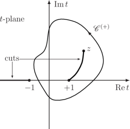
Figure 1: The complex $t$-plane and the integration contour $\mathscr{C}^{(+)}$ for Eq. (1.1) and for the definition (3.1) of the associated Legendre function $P_{\nu}^{\pm m}(z)$ of the first kind of integer order. The cut joining the points $t=+1$ and $t=z$ (being two out of four branch points of the integrands in Eqs. (1.1) and (3.1)) is the circular arc (3.3).

Using the representation (1.1), we have re-derived the Rodrigues-type formula

$$\frac{\partial P_{\nu}(z)}{\partial\nu}\bigg{|}_{\nu=n}=-P_{n}(z)\ln\frac{z+1}{2}+\frac{1}{2^{n-1}n!}\frac{\mathrm{d}^{n}}{\mathrm{d}z^{n}}\left[(z^{2}-1)^{n}\ln\frac{z+1}{2}\right]\qquad(n\in\mathbb{N}),$$ (1.2)

which was first obtained long ago by Jolliffe [2] with no resort to the complex integration technique. Then we have shown that $[\partial P_{\nu}(z)/\partial\nu]_{\nu=n}$ may be written as

$$\frac{\partial P_{\nu}(z)}{\partial\nu}\bigg{|}_{\nu=n}=P_{n}(z)\ln\frac{z+1}{2}+R_{n}(z),$$ (1.3)

where $P_{n}(z)$ is a Legendre polynomial and $R_{n}(z)$ is a polynomial in $z$ of degree $n$. Using various techniques, we have found several explicit representations of $R_{n}(z)$. In addition to the representation

$$R_{n}(z)=2[\psi(2n+1)-\psi(n+1)]P_{n}(z)+2\sum_{k=0}^{n-1}(-)^{k+n}\frac{2k+1}{(n-k)(k+n+1)}P_{k}(z),$$ (1.4)

which is a slight modification of the one found by Bromwich [3], and the representation

$$R_{n}(z)=-2\psi(n+1)P_{n}(z)+2\sum_{k=0}^{n}\frac{(k+n)!\psi(k+n+1)}{(k!)^{2}(n-k)!}\left(\frac{z-1}{2}\right)^{k}$$ (1.5)

due to Schelkunoff [4], we have obtained the formula

$$R_{n}(z)=2\sum_{k=0}^{n}(-)^{k+n}\frac{(k+n)!}{(k!)^{2}(n-k)!}[\psi(k+n+1)-\psi(k+1)]\left(\frac{z+1}{2}\right)^{k}.$$ (1.6)

Here and henceforth,

$$\psi(\zeta)=\frac{1}{\Gamma(\zeta)}\frac{\mathrm{d}\Gamma(\zeta)}{\mathrm{d}\zeta}$$ (1.7)

denotes the digamma function [5, 6, 7].

Still more recently, in the addendum [8], we have exploited the Jolliffe’s formula (1.2) to present a derivation of Eq. (1.6) being much simpler than the original one in [1]. In addition, Eq. (1.2) has been used to obtain two further new representations of $R_{n}(z)$, namely

$$R_{n}(z)=2\psi(n+1)P_{n}(z)-2\left(\frac{z+1}{2}\right)^{n}\sum_{k=0}^{n}{n\choose k}^{2}\psi(n-k+1)\left(\frac{z-1}{z+1}\right)^{k}$$ (1.8)

and

$$R_{n}(z)=2\psi(n+1)P_{n}(z)-2\left(\frac{z-1}{2}\right)^{n}\sum_{k=0}^{n}{n\choose k}^{2}\psi(k+1)\left(\frac{z+1}{z-1}\right)^{k}.$$ (1.9)

In the course of solving boundary value problems of theoretical acoustics, electromagnetism, heat conduction and some other branches of theoretical physics and applied mathematics (cf, e.g., [9, 10, 11, 12, 13, 14, 15, 16, 17, 18, 19, 20, 21, 22, 23, 25, 24, 26, 27, 28]), one occasionally encounters the derivative of the associated Legendre function of the first kind [29, 30, 31, 32, 33, 34, 35, 36, 37, 38, 39, 40, 41, 42, 43, 44, 45, 46, 47, 48, 49, 50, 51, 6, 7, 52, 53, 54, 55, 56, 57, 58] of integer order with respect to its degree, $\partial P_{\nu}^{\pm m}(z)/\partial\nu$ with $m\in\mathbb{N}$. We have found that except for the case of $m=0$ studied in [1, 8], thus far this derivative has not been a subject of a systematic, exhaustive investigation and that the relevant knowledge is very incomplete (cf section 2). It is the purpose of the present paper to fill in this gap and to give an extension of our previously-obtained results for $\partial P_{\nu}(z)/\partial\nu$ to the case of $\partial P_{\nu}^{\pm m}(z)/\partial\nu$. In particular, we shall extensively investigate the functions $[\partial P_{\nu}^{\pm m}(z)/\partial\nu]_{\nu=n}$ with $n\in\mathbb{N}$. Besides being interesting for their own sake and potentially useful for applications to the problems mentioned above, the results will also allow us to contribute to the theory of the associated Legendre function of the second kind of integer degree and order, $Q_{n}^{\pm m}(z)$. In a simple manner, we shall obtain several representations, both explicit and of the Rodrigues type, of the latter function for various ranges of $n$ and $m$; we believe that some of these representations are new. The explicit expressions we provide for both $[\partial P_{\nu}^{\pm m}(z)/\partial\nu]_{\nu=n}$ and $Q_{n}^{\pm m}(z)$ are suitable for use for numerical purposes in various regions of the complex $z$-plane.

The structure of the paper is as follows. Section 2 provides a summary of fragmentary research on $\partial P_{\nu}^{\mu}(z)/\partial\nu$ done thus far by other authors. In section 3, we make an overview of these properties of the associated Legendre function of the first kind of integer order, $P_{\nu}^{\pm m}(z)$, which will find applications in later parts of the work. In section 4, we find several contour-integral representations of $\partial P_{\nu}^{\pm m}(z)/\partial\nu$. In section 5, we investigate $[\partial P_{\nu}^{\pm m}(z)/\partial\nu]_{\nu=n}$ with $n\in\mathbb{N}$, the cases $0\leqslant m\leqslant n$ and $m>n$ being considered separately. In each of these two cases, at first we use contour integrals for $[\partial P_{\nu}^{\pm m}(z)/\partial\nu]_{\nu=n}$ to obtain Rodrigues-type formulas for this function. Then, these formulas are used to construct several closed-form representations of $[\partial P_{\nu}^{\pm m}(z)/\partial\nu]_{\nu=n}$. Applications of the results of section 5 to the construction of some representations of the associated Legendre function of the second kind of integer degree and order constitute section 6.1, while in sections 6.2 and 6.3 the derivatives $[\partial^{2}P_{\nu}^{m}(z)/\partial\nu^{2}]_{\nu=n}$, $[\partial Q_{\nu}^{m}(z)/\partial\nu]_{\nu=n}$ and $[\partial Q_{\nu}^{m}(z)/\partial\nu]_{\nu=-n-1}$, all with $m>n$, are expressed in terms of $[\partial P_{\nu}^{-m}(\pm z)/\partial\nu]_{\nu=n}$. The paper ends with an appendix, in which some formulas for the Jacobi polynomials, exploited in sections 3 and 5, are listed.

Throughout the paper, we shall be adopting the standard convention, according to which $z\in\mathbb{C}\setminus[-1,1]$, with the phases restricted by

$$-\pi<\arg(z)<\pi,\qquad-\pi<\arg(z\pm 1)<\pi$$ (1.10)

(this corresponds to drawing a cut in the $z$-plane along the real axis from $z=+1$ to $z=-\infty$), hence,

$$-z=\mathrm{e}^{\mp\mathrm{i}\pi}z\qquad-z+1=\mathrm{e}^{\mp\mathrm{i}\pi}(z-1)\qquad-z-1=\mathrm{e}^{\mp\mathrm{i}\pi}(z+1)\qquad(\arg(z)\gtrless 0).$$ (1.11)

Also, it will be implicit that $x\in[-1,1]$, $\nu\in\mathbb{C}$, $\mu\in\mathbb{C}$, $n\in\mathbb{N}$, $m\in\mathbb{N}$. Finally, it will be understood that if the upper limit of a sum is less by unity than the lower one, then the sum vanishes identically.

The definitions of the associated Legendre functions of the first and second kinds used in the paper are those of Hobson [40].

The present paper may be considered as a complement to [59], where the derivative $\partial P_{n}^{\mu}(z)/\partial\mu$ has been investigated exhaustively.

2 Overview of research done on $\partial P_{\nu}^{\mu}(z)/\partial\nu$ and $\partial P_{\nu}^{\mu}(x)/\partial\nu$

An overview of the research done on $\partial P_{\nu}^{0}(z)/\partial\nu$ ($\equiv\partial P_{\nu}(z)/\partial\nu$) was presented in [1]; to the references cited therein, one should add the works [16, 60, 61, 62, 63, 64, 21, 65, 66, 67, 26, 68, 69, 70]. As regards the derivative $\partial P_{\nu}^{\mu}(z)/\partial\nu$ with $\mu\neq 0$, our literature search showed very few results. Robin [71] (cf also [46, pp. 170–4]), differentiating term by term the following series representation of $P_{\nu}^{\mu}(z)$ [6, 7]:

$$P_{\nu}^{\mu}(z)=\left(\frac{z+1}{z-1}\right)^{\mu/2}\sum_{k=0}^{\infty}\frac{\Gamma(k+\nu+1)}{k!\Gamma(\nu-k+1)\Gamma(k-\mu+1)}\left(\frac{z-1}{2}\right)^{k}\qquad(|z-1|<2)$$ (2.1)

arrived at the formula

$$\frac{\partial P_{\nu}^{\mu}(z)}{\partial\nu} = \left(\frac{z+1}{z-1}\right)^{\mu/2}\sum_{k=1}^{\infty}\frac{\Gamma(k+\nu+1)}{k!\Gamma(\nu-k+1)\Gamma(k-\mu+1)}$$ (2.2)

$$\times[\psi(k+\nu+1)-\psi(\nu-k+1)]\left(\frac{z-1}{2}\right)^{k}\qquad(|z-1|<2).$$

If in Eq. (2.2) one makes use of the well-known [5, 6, 7] identities

$$\Gamma(\zeta)\Gamma(1-\zeta)=\frac{\pi}{\sin(\pi\zeta)}$$ (2.3)

and

$$\psi(\zeta)=\psi(1-\zeta)-\pi\cot(\pi\zeta)$$ (2.4)

and exploits Eq. (2.1), this yields [6, page 178]

$$\frac{\partial P_{\nu}^{\mu}(z)}{\partial\nu} = \pi\cot(\pi\nu)P_{\nu}^{\mu}(z)-\frac{\sin(\pi\nu)}{\pi}\left(\frac{z+1}{z-1}\right)^{\mu/2}\sum_{k=0}^{\infty}(-)^{k}\frac{\Gamma(k+\nu+1)\Gamma(k-\nu)}{k!\Gamma(k-\mu+1)}$$ (2.5)

$$\times[\psi(k+\nu+1)-\psi(k-\nu)]\left(\frac{z-1}{2}\right)^{k}\qquad(|z-1|<2).$$

Manipulating with the series on the right-hand side of the above formula, Robin [46, 71] showed that for $\nu=n$ the formula goes over into

$$\frac{\partial P_{\nu}^{\mu}(z)}{\partial\nu}\bigg{|}_{\nu=n} = \left(\frac{z+1}{z-1}\right)^{\mu/2}\sum_{k=1}^{n}\frac{(k+n)!}{k!(n-k)!\Gamma(k-\mu+1)}$$ (2.8)

$$\quad\times[\psi(k+n+1)-\psi(n-k+1)]\left(\frac{z-1}{2}\right)^{k}$$

$$+\,\frac{(2n+1)!}{(n+1)!\Gamma(n-\mu+2)}\left(\frac{z+1}{z-1}\right)^{\mu/2}\left(\frac{z-1}{2}\right)^{n+1}$$

$$\quad\times{}_{3}F_{2}\left(\begin{array}[]{c}1,1,2n+2\\ n+2,n+2-\mu\end{array};\frac{1-z}{2}\right),$$

with ${}_{3}F_{2}$ being a generalized hypergeometric function. In the particular case of $n=0$, the finite sum on the right-hand side of Eq. (2.8) vanishes, while the ${}_{3}F_{2}$ function appearing therein reduces to ${}_{2}F_{1}(1,1;2-\mu;(1-z)/2)$, so that the equation goes over into [6, p. 177]

$$\frac{\partial P_{\nu}^{\mu}(z)}{\partial\nu}\bigg{|}_{\nu=0}=\frac{z-1}{2\Gamma(2-\mu)}\left(\frac{z+1}{z-1}\right)^{\mu/2}{}_{2}F_{1}\left(1,1;2-\mu;\frac{1-z}{2}\right).$$ (2.10)

For the sake of completeness, we mention here that a formula for $[\partial P_{\nu}^{\mu}(z)/\partial\nu]_{\nu=n-1/2}$, which we do not display here, has been provided by Brychkov in [58].

Results on $\partial P_{\nu}^{\mu}(x)/\partial\nu$ are also scarce and fragmentary. A formula analogous to Eq. (2.2) may be found in [7, p. 1026] and [52, p. 94]. Counterparts of Eqs. (2.5) and (2.10) are given in [6] on pp. 178 and 177, respectively. Closed-form expressions for $[\partial P_{\nu}^{-1}(x)/\partial\nu]_{\nu=0}$ and $[\partial P_{\nu}^{-1}(x)/\partial\nu]_{\nu=1}$ are presented in [7, pp. 1026–7], [52, p. 94] and [55, p. 335]. Tsu [73] found explicit representations of $[\partial P_{\nu}^{0}(x)/\partial\nu]_{\nu=0}$ ($\equiv[\partial P_{\nu}(x)/\partial\nu]_{\nu=0}$) and $[\partial P_{\nu}^{1}(x)/\partial\nu]_{\nu=0}$ and provided the recursive relation

$$(1-x^{2})^{1/2}\frac{\partial P_{\nu}^{m+1}(x)}{\partial\nu}\bigg{|}_{\nu=n}-(n-m)x\frac{\partial P_{\nu}^{m}(x)}{\partial\nu}\bigg{|}_{\nu=n}+(n+m)\frac{\partial P_{\nu}^{m}(x)}{\partial\nu}\bigg{|}_{\nu=n-1}$$

$$=xP_{n}^{m}(x)-P_{n-1}^{m}(x),$$ (2.11)

enabling one to generate $[\partial P_{\nu}^{m}(x)/\partial\nu]_{\nu=n}$ for other values of $n$ and $m$; however, no general formula for $[\partial P_{\nu}^{m}(x)/\partial\nu]_{\nu=n}$ was given in that work. Finally, in a study on the Dirichlet averages of $x^{t}\ln x$, Carlson [74] arrived at the following closed-form representation of $[\partial P_{\nu}^{-m}(x)/\partial\nu]_{\nu=n}$ with $0\leqslant m\leqslant n$:

$$\frac{\partial P_{\nu}^{-m}(x)}{\partial\nu}\bigg{|}_{\nu=n} = P_{n}^{-m}(x)\ln\frac{1+x}{2}-[\psi(n+m+1)+\psi(n+1)]P_{n}^{-m}(x)$$

$$+\,\frac{(n-m)!}{(n+m)!}\left(\frac{1-x^{2}}{4}\right)^{m/2}$$

$$\quad\times\sum_{k=0}^{n-m}(-)^{k}\frac{(k+n+m)!\psi(k+n+m+1)}{k!(k+m)!(n-m-k)!}\left(\frac{1-x}{2}\right)^{k}$$

$$+\,\left(\frac{1-x}{1+x}\right)^{m/2}\sum_{k=0}^{n}(-)^{k}\frac{(k+n)!\psi(k+n+1)}{k!(k+m)!(n-k)!}\left(\frac{1-x}{2}\right)^{k}\qquad(0\leqslant m\leqslant n)$$

and proved the identity

$$\frac{\partial P_{\nu}^{m}(x)}{\partial\nu}\bigg{|}_{\nu=n} = (-)^{m}\frac{(n+m)!}{(n-m)!}\frac{\partial P_{\nu}^{-m}(x)}{\partial\nu}\bigg{|}_{\nu=n}$$ (2.13)

$$+\,[\psi(n+m+1)-\psi(n-m+1)]P_{n}^{m}(x)\qquad(0\leqslant m\leqslant n);$$

in addition, he showed that

$$\frac{\partial P_{\nu}^{-m}(x)}{\partial\nu}\bigg{|}_{\nu=0} = (-)^{m}P_{0}^{-m}(-x)\ln\frac{1+x}{2}$$

$$+\,\psi(1)P_{0}^{-m}(x)-(-)^{m}\psi(m+1)P_{0}^{-m}(-x)$$

$$+\,(-)^{m}\left(\frac{1-x^{2}}{4}\right)^{-m/2}\sum_{k=0}^{m-1}(-)^{k}\frac{\psi(m-k+1)}{k!(m-k)!}\left(\frac{1-x}{2}\right)^{k}\qquad(m>0).$$

3 Definition and some relevant properties of the associated Legendre function of the first kind of integer order

In this section, we shall present these properties of the associated Legendre function of the first kind of integer order which will find applications in later parts of this paper.

3.1 Function of arbitrary degree

The associated Legendre function of the first kind of complex degree $\nu$ and integer order $\pm m$ may be defined as the following generalization of the Schläfli contour integral [40, p. 191]:

$$P_{\nu}^{\pm m}(z)=\frac{\Gamma(\nu\pm m+1)}{\Gamma(\nu+1)}\frac{1}{2^{\nu+1}\pi\mathrm{i}}(z^{2}-1)^{\pm m/2}\oint_{\mathscr{C}^{(+)}}\mathrm{d}t\>\frac{(t^{2}-1)^{\nu}}{(t-z)^{\nu\pm m+1}}.$$ (3.1)

The integration path $\mathscr{C}^{(+)}$, shown in Fig. 1, is a closed circuit enclosing the points $t=+1$ and $t=z$ in the counter-clockwise sense. If $\nu$ is not an integer, the integrand has four branch points located at $t=\pm 1$, $t=z$ and $|t|=\infty$. To make the integrand single-valued, we make two cuts in the $t$-plane. The first one is

$$t_{\mathrm{cut}}=-\eta\qquad(1\leqslant\eta<\infty),$$ (3.2)

which is the semi-line drawn along the negative real semi-axis from $t=-1$ to $t=-\infty$. The second one is the curve

$$t_{\mathrm{cut}}=\frac{1+\eta z}{z+\eta}\qquad(1\leqslant\eta<\infty)$$ (3.3)

joining the points $t=+1$ and $t=z$. It is seen to be that out of two circular arcs of radius

$$\rho=\sqrt{1+\left(\frac{|z|^{2}-1}{2\textrm{Im}(z)}\right)^{2}},$$ (3.4)

centered at

$$t_{0}=\mathrm{i}\,\frac{|z|^{2}-1}{2\textrm{Im}(z)}$$ (3.5)

and connecting the points $t=+1$ and $t=z$, which does not go through the point $t=-1$. The contour $\mathscr{C}^{(+)}$ is not to cross any of the two cuts (3.2) and (3.3). The phases in the integrand in Eq. (3.1) are stipulated as follows: at the point on the right to $t=+1$ (and on the right to $z$ if the latter be real), where the path $\mathscr{C}^{(+)}$ crosses the real axis, we set $\arg(t\pm 1)=0$ and $|\arg(t-z)|<\pi$. In the plane with the cross-cut along the real axis from $z=+1$ to $z=-\infty$ (cf the remark below Eq. (1.10)), the function $P_{\nu}^{\pm m}(z)$ is single-valued.

It is seen from Eq. (3.1) that

$$P_{\nu}^{m}(z)=(z^{2}-1)^{m/2}\frac{\mathrm{d}^{m}P_{\nu}(z)}{\mathrm{d}z^{m}},$$ (3.6)

where $P_{\nu}(z)\equiv P_{\nu}^{0}(z)$ is the Legendre function of the first kind.

It may be shown [40] that $P_{\nu}^{\pm m}(z)$ possesses the property

$$P_{-\nu-1}^{\pm m}(z)=P_{\nu}^{\pm m}(z).$$ (3.7)

Replacing in Eq. (3.1) $\nu$ with $-\nu-1$, exploiting the fact that

$$\frac{\Gamma(-\nu\pm m)}{\Gamma(-\nu)}=(-)^{m}\frac{\Gamma(\nu+1)}{\Gamma(\nu\mp m+1)}$$ (3.8)

and making use of Eq. (3.7), yields

$$P_{\nu}^{\pm m}(z)=(-)^{m}\frac{\Gamma(\nu+1)}{\Gamma(\nu\mp m+1)}\frac{2^{\nu}}{\pi\mathrm{i}}(z^{2}-1)^{\pm m/2}\oint_{\mathscr{C}^{(+)}}\mathrm{d}t\>\frac{(t-z)^{\nu\mp m}}{(t^{2}-1)^{\nu+1}}.$$ (3.9)

If in Eq. (3.9) we change the integration variable from $t$ to

$$u=-1+2\frac{z+1}{t+1},$$ (3.10)

this results in

$$P_{\nu}^{\pm m}(z)=\frac{\Gamma(\nu+1)}{\Gamma(\nu\mp m+1)}\frac{1}{2^{\nu+1}\pi\mathrm{i}}\left(\frac{z-1}{z+1}\right)^{\pm m/2}\oint_{\mathscr{C}^{\prime\,(+)}}\mathrm{d}u\>\frac{(u-1)^{\nu\mp m}(u+1)^{\nu\pm m}}{(u-z)^{\nu+1}}.$$ (3.11)

The contour $\mathscr{C}^{\prime\,(+)}$ surrounds the points $u=+1$ and $u=z$ in the counter-clockwise sense and does not cross either of the two straight-line cuts

$$u_{\mathrm{cut}}=-1+2\frac{z+1}{1-\eta}\qquad(1\leqslant\eta<\infty)$$ (3.12)

and

$$u_{\mathrm{cut}}=1+2\frac{z-1}{1+\eta}\qquad(1\leqslant\eta<\infty).$$ (3.13)

Likewise, if in Eq. (3.9) the variable $t$ is replaced by

$$u=1-2\frac{z-1}{t-1},$$ (3.14)

one finds

$$P_{\nu}^{\pm m}(z)=\frac{\Gamma(\nu+1)}{\Gamma(\nu\mp m+1)}\frac{1}{2^{\nu+1}\pi\mathrm{i}}\left(\frac{z+1}{z-1}\right)^{\pm m/2}\oint_{\mathscr{C}^{\prime\prime\,(+)}}\mathrm{d}u\>\frac{(u-1)^{\nu\pm m}(u+1)^{\nu\mp m}}{(u-z)^{\nu+1}},$$ (3.15)

where the path $\mathscr{C}^{\prime\prime\,(+)}$ encloses the points $u=+1$ and $u=z$ in the counter-clockwise sense and also does not cross the cuts (3.12) and (3.13). It is evident that the contour $\mathscr{C}^{\prime\prime\,(+)}$ may be deformed into the contour $\mathscr{C}^{\prime\,(+)}$ without changing the value of the integral in Eq. (3.15), i.e., it holds that

$$P_{\nu}^{\pm m}(z)=\frac{\Gamma(\nu+1)}{\Gamma(\nu\mp m+1)}\frac{1}{2^{\nu+1}\pi\mathrm{i}}\left(\frac{z+1}{z-1}\right)^{\pm m/2}\oint_{\mathscr{C}^{\prime\,(+)}}\mathrm{d}u\>\frac{(u-1)^{\nu\pm m}(u+1)^{\nu\mp m}}{(u-z)^{\nu+1}}.$$ (3.16)

As a corollary, from Eqs. (3.11) and (3.16) one obtains the relation

$$P_{\nu}^{-m}(z)=\frac{\Gamma(\nu-m+1)}{\Gamma(\nu+m+1)}P_{\nu}^{m}(z).$$ (3.17)

If this is combined with Eq. (3.9), this results in

$$P_{\nu}^{\pm m}(z)=(-)^{m}\frac{\Gamma(\nu+1)}{\Gamma(\nu\mp m+1)}\frac{2^{\nu}}{\pi\mathrm{i}}(z^{2}-1)^{\mp m/2}\oint_{\mathscr{C}^{(+)}}\mathrm{d}t\>\frac{(t-z)^{\nu\pm m}}{(t^{2}-1)^{\nu+1}}.$$ (3.18)

(It is worthwhile to add that Eq. (3.18) may be also obtained from equation (3.9) by subjecting the integral in the latter to the variable transformation (4.2) and deforming suitably the resulting integration contour. Then Eq. (3.17) appears to be a corollary from Eqs. (3.9) and (3.18).)

On the cut $-1\leqslant x\leqslant+1$, after Hobson [40], it is customary to define

$$P_{\nu}^{\pm m}(x) = \mathrm{e}^{\pm\mathrm{i}\pi m/2}P_{\nu}^{\pm m}(x+\mathrm{i}0)=\mathrm{e}^{\mp\mathrm{i}\pi m/2}P_{\nu}^{\pm m}(x-\mathrm{i}0)$$ (3.19)

$$= \frac{1}{2}\left[\mathrm{e}^{\pm\mathrm{i}\pi m/2}P_{\nu}^{\pm m}(x+\mathrm{i}0)+\mathrm{e}^{\mp\mathrm{i}\pi m/2}P_{\nu}^{\pm m}(x-\mathrm{i}0)\right].$$

3.2 Function of integer degree

If $\nu=n$, the cut (3.3) in the definition of the contour integral (3.1) is unnecessary and may be removed. Then, by the theory of residues, from Eq. (3.1) one has the Rodrigues-type formula

$$P_{n}^{\pm m}(z)=\frac{1}{2^{n}n!}(z^{2}-1)^{\pm m/2}\frac{\mathrm{d}^{n\pm m}}{\mathrm{d}z^{n\pm m}}(z^{2}-1)^{n},$$ (3.20)

subject to the constraint $0\leqslant m\leqslant n$ if the lower signs are chosen. If Eq. (3.20) is combined with

$$P_{n}^{-m}(z)=\frac{(n-m)!}{(n+m)!}P_{n}^{m}(z)\qquad(0\leqslant m\leqslant n),$$ (3.21)

which is the direct consequence of Eq. (3.17), this yields

$$P_{n}^{\pm m}(z)=\frac{1}{2^{n}n!}\frac{(n\pm m)!}{(n\mp m)!}(z^{2}-1)^{\mp m/2}\frac{\mathrm{d}^{n\mp m}}{\mathrm{d}z^{n\mp m}}(z^{2}-1)^{n}\qquad(0\leqslant m\leqslant n).$$ (3.22)

For $m>n$, Eq. (3.20) implies

$$P_{n}^{m}(z)=0\qquad(m>n).$$ (3.23)

Another property of $P_{n}^{\pm m}(z)$, which shall prove to be useful in later considerations, is

$$P_{n}^{\pm m}(-z)=(-)^{n}P_{n}^{\pm m}(z)\qquad(0\leqslant m\leqslant n).$$ (3.24)

This may be obtained from Eq. (3.20), with the aid of the relations (1.11).

Other Rodrigues-type representations of $P_{n}^{\pm m}(z)$ may be obtained by applying the theory of residues to the contour integrals (3.11) and (3.16), after setting therein $\nu=n$ and removing, now redundant, the cut (3.13). For $0\leqslant m\leqslant n$, this renders two formulas

$$P_{n}^{\pm m}(z)=\frac{1}{2^{n}(n\mp m)!}\left(\frac{z-1}{z+1}\right)^{\pm m/2}\frac{\mathrm{d}^{n}}{\mathrm{d}z^{n}}\left[(z-1)^{n\mp m}(z+1)^{n\pm m}\right]\qquad(0\leqslant m\leqslant n)$$ (3.25)

and

$$P_{n}^{\pm m}(z)=\frac{1}{2^{n}(n\mp m)!}\left(\frac{z+1}{z-1}\right)^{\pm m/2}\frac{\mathrm{d}^{n}}{\mathrm{d}z^{n}}\left[(z-1)^{n\pm m}(z+1)^{n\mp m}\right]\qquad(0\leqslant m\leqslant n),$$ (3.26)

obtained originally by Schendel [75] in a different way. If $m>n$, proceeding in the analogous way, from Eq. (3.11) one finds

$$P_{n}^{-m}(z)=\frac{1}{2^{n}(n+m)!}\left(\frac{z+1}{z-1}\right)^{m/2}\frac{\mathrm{d}^{n}}{\mathrm{d}z^{n}}\left[(z-1)^{n+m}(z+1)^{n-m}\right]\qquad(m>n).$$ (3.27)

For the sake of later applications, we shall derive here still another Rodrigues-type representation of $P_{n}^{-m}(z)$ valid for $m>n$. To this end, at first we observe that if the lower signs are chosen in Eq. (3.18) and if one sets $\nu=n$, the integrand in the resulting equation becomes single-valued in the domain enclosed by the contour $\mathscr{C}^{(+)}$ and is seen to possess two poles in this region: one of order $n+1$, located at $t=+1$, and the other, of order $m-n$, located at $t=z$. Thus, we may remove the cut (3.3) and, by the Cauchy theorem, write

$$P_{n}^{-m}(z) = (-)^{m}\frac{n!}{(n+m)!}\frac{2^{n}}{\pi\mathrm{i}}(z^{2}-1)^{m/2}\oint_{\mathscr{C}_{+1}^{(+)}}\mathrm{d}t\>\frac{(t-z)^{n-m}}{(t^{2}-1)^{n+1}}$$ (3.28)

$$+\,(-)^{m}\frac{n!}{(n+m)!}\frac{2^{n}}{\pi\mathrm{i}}(z^{2}-1)^{m/2}\oint_{\mathscr{C}_{z}^{(+)}}\mathrm{d}t\>\frac{(t-z)^{n-m}}{(t^{2}-1)^{n+1}}\qquad(m>n).$$

Here, the path $\mathscr{C}_{+1}^{(+)}$ surrounds the point $t=+1$ in the positive direction and leaves the points $t=-1$ and $t=z$ outside, while the contour $\mathscr{C}_{z}^{(+)}$ encloses the point $t=z$, is run in the positive sense, with the points $t=\pm 1$ located exterior to it; none of the two paths crosses the cut (3.2). Instead of applying the theory of residues already at this stage, we subject the first integral in Eq. (3.28) to the variable transformation (3.10). This gives

$$P_{n}^{-m}(z) = \frac{n!}{(n+m)!}\frac{1}{2^{n+1}\pi\mathrm{i}}\left(\frac{z-1}{z+1}\right)^{m/2}\oint_{\mathscr{C}_{z}^{\prime\,(+)}}\mathrm{d}u\>\frac{(u-1)^{n-m}(u+1)^{n+m}}{(u-z)^{n+1}}$$ (3.29)

$$+\,(-)^{m}\frac{n!}{(n+m)!}\frac{2^{n}}{\pi\mathrm{i}}(z^{2}-1)^{m/2}\oint_{\mathscr{C}_{z}^{(+)}}\mathrm{d}t\>\frac{(t-z)^{n-m}}{(t^{2}-1)^{n+1}}\qquad(m>n),$$

where the contour $\mathscr{C}_{z}^{\prime\,(+)}$ encircles the point $u=z$ counter-clockwise, does not enclose the points $u=\pm 1$ and also does not cross the cut (3.12). Applying now the theory of residues to Eq. (3.29), we obtain

$$P_{n}^{-m}(z) = \frac{1}{2^{n}(n+m)!}\left(\frac{z-1}{z+1}\right)^{m/2}\frac{\mathrm{d}^{n}}{\mathrm{d}z^{n}}\left[(z-1)^{n-m}(z+1)^{n+m}\right]$$

$$+\,(-)^{m}\frac{2^{n+1}n!}{(n+m)!(m-n-1)!}(z^{2}-1)^{m/2}\frac{\mathrm{d}^{m-n-1}}{\mathrm{d}z^{m-n-1}}(z^{2}-1)^{-n-1}\qquad(m>n),$$

which is the desired result. Comparison with Eq. (3.27) shows that the first term on the right-hand side of Eq. (LABEL:3.30) equals $(-)^{n}P_{n}^{-m}(-z)$ (with $m>n$), and consequently

$$P_{n}^{-m}(z) = (-)^{n}P_{n}^{-m}(-z)$$

$$+\,(-)^{m}\frac{2^{n+1}n!}{(n+m)!(m-n-1)!}(z^{2}-1)^{m/2}\frac{\mathrm{d}^{m-n-1}}{\mathrm{d}z^{m-n-1}}(z^{2}-1)^{-n-1}\qquad(m>n).$$

Combining Eqs. (3.20), (3.22), (3.25) to (3.27) and (LABEL:3.31) with Eq. (A.1) and using, whenever necessary, Eqs. (3.21) and (3.24), yields the following formulas relating the Legendre function considered here to particular Jacobi polynomials:

$$P_{n}^{m}(z)=\frac{n!}{(n-m)!}\left(\frac{z+1}{z-1}\right)^{m/2}P_{n}^{(-m,m)}(z)\qquad(0\leqslant m\leqslant n),$$ (3.32)

$$P_{n}^{-m}(-z)=(-)^{n}\frac{n!}{(n+m)!}\left(\frac{z+1}{z-1}\right)^{m/2}P_{n}^{(-m,m)}(z),$$ (3.33)

$$P_{n}^{m}(z)=\frac{n!}{(n-m)!}\left(\frac{z-1}{z+1}\right)^{m/2}P_{n}^{(m,-m)}(z)\qquad(0\leqslant m\leqslant n),$$ (3.34)

$$P_{n}^{-m}(z)=\frac{n!}{(n+m)!}\left(\frac{z-1}{z+1}\right)^{m/2}P_{n}^{(m,-m)}(z),$$ (3.35)

$$P_{n}^{m}(z)=\frac{(n+m)!}{n!}\left(\frac{z^{2}-1}{4}\right)^{-m/2}P_{n+m}^{(-m,-m)}(z)\qquad(0\leqslant m\leqslant n),$$ (3.36)

$$P_{n}^{m}(z)=\frac{(n+m)!}{n!}\left(\frac{z^{2}-1}{4}\right)^{m/2}P_{n-m}^{(m,m)}(z)\qquad(0\leqslant m\leqslant n),$$ (3.37)

$$P_{n}^{-m}(z)-(-)^{n}P_{n}^{-m}(-z)=(-)^{m}\frac{n!}{(n+m)!}\left(\frac{z^{2}-1}{4}\right)^{-m/2}P_{m-n-1}^{(-m,-m)}(z)\qquad(m>n).$$ (3.38)

We shall make extensive use of the above formulas in sections 5.1.2 and 5.4.2.

4 Contour-integral representations of $\partial P_{\nu}^{\pm m}(z)/\partial\nu$

We begin our investigations on the derivative $\partial P_{\nu}^{\pm m}(z)/\partial\nu$ with the derivation of its several contour-integral representations.

Differentiation of Eq. (3.1) with respect to $\nu$ gives the first such representation:

$$\frac{\partial P_{\nu}^{\pm m}(z)}{\partial\nu} = [\psi(\nu\pm m+1)-\psi(\nu+1)]P_{\nu}^{\pm m}(z)$$

$$+\,\frac{\Gamma(\nu\pm m+1)}{\Gamma(\nu+1)}\frac{1}{2^{\nu+1}\pi\mathrm{i}}(z^{2}-1)^{\pm m/2}\oint_{\mathscr{C}^{(+)}}\mathrm{d}t\>\frac{(t^{2}-1)^{\nu}}{(t-z)^{\nu\pm m+1}}\ln\frac{t^{2}-1}{2(t-z)}.$$

Consider now the following linear fractional transformation:

$$s=-1+(z+1)\frac{t-1}{t-z}.$$ (4.2)

It maps the complex $t$-plane onto the complex $s$-plane. In particular, the points $t=-1$, $+1$, $z$ and $\infty$ are mapped onto the points $s=+1$, $-1$, $\infty$ and $z$, respectively, the cut (3.2) is mapped onto the cut

$$s_{\mathrm{cut}}=\frac{1+\eta z}{z+\eta}\qquad(1\leqslant\eta<\infty)$$ (4.3)

and the cut (3.3) onto the cut

$$s_{\mathrm{cut}}=-\eta\qquad(1\leqslant\eta<\infty).$$ (4.4)

In addition, the path $\mathscr{C}^{(+)}$ is mapped onto the contour $\mathscr{C}^{\prime\prime\prime\,(-)}$, which encloses the points $s=1$ and $s=z$ in the clock-wise sense and does not cross any of the two cuts (4.3) and (4.4).

To obtain the second representation of $\partial P_{\nu}^{\pm m}(z)/\partial\nu$, we rewrite Eq. (LABEL:4.1) in the form

$$\frac{\partial P_{\nu}^{\pm m}(z)}{\partial\nu} = [\psi(\nu\pm m+1)-\psi(\nu+1)]P_{\nu}^{\pm m}(z)$$ (4.5)

$$+\,\frac{\Gamma(\nu\pm m+1)}{\Gamma(\nu+1)}\frac{1}{2^{\nu+1}\pi\mathrm{i}}(z^{2}-1)^{\pm m/2}\oint_{\mathscr{C}^{(+)}}\mathrm{d}t\>\frac{(t^{2}-1)^{\nu}}{(t-z)^{\nu\pm m+1}}\ln\frac{t+1}{2}$$

$$+\frac{\Gamma(\nu\pm m+1)}{\Gamma(\nu+1)}\frac{1}{2^{\nu+1}\pi\mathrm{i}}(z^{2}-1)^{\pm m/2}\oint_{\mathscr{C}^{(+)}}\mathrm{d}t\>\frac{(t^{2}-1)^{\nu}}{(t-z)^{\nu\pm m+1}}\ln\frac{t-1}{t-z}.$$

Let us look closer at the second integral on the right-hand side of Eq. (4.5), which is

$$I_{\nu}^{\pm m}(z)=\frac{\Gamma(\nu\pm m+1)}{\Gamma(\nu+1)}\frac{1}{2^{\nu+1}\pi\mathrm{i}}(z^{2}-1)^{\pm m/2}\oint_{\mathscr{C}^{(+)}}\mathrm{d}t\>\frac{(t^{2}-1)^{\nu}}{(t-z)^{\nu\pm m+1}}\ln\frac{t-1}{t-z}.$$ (4.6)

Subjecting this integral to the transformation (4.2) results in

$$I_{\nu}^{\pm m}(z)=-\frac{\Gamma(\nu\pm m+1)}{\Gamma(\nu+1)}\frac{1}{2^{\nu+1}\pi\mathrm{i}}(z^{2}-1)^{\mp m/2}\oint_{\mathscr{C}^{\prime\prime\prime\,(-)}}\mathrm{d}s\>\frac{(s^{2}-1)^{\nu}}{(s-z)^{\nu\mp m+1}}\ln\frac{s+1}{z+1}.$$ (4.7)

If in Eq. (4.7) we change the name of the integration variable from $s$ to $t$, then switch from the contour $\mathscr{C}^{\prime\prime\prime\,(-)}$ to the oppositely traversed contour $\mathscr{C}^{\prime\prime\prime\,(+)}$ and deform the latter into the path $\mathscr{C}^{(+)}$ (because of the structure of the integrand, this deformation does not change the value of the integral in question), after subsequent use of Eq. (3.1), we obtain

$$I_{\nu}^{\pm m}(z) = \frac{\Gamma(\nu\pm m+1)}{\Gamma(\nu+1)}\frac{1}{2^{\nu+1}\pi\mathrm{i}}(z^{2}-1)^{\mp m/2}\oint_{\mathscr{C}^{(+)}}\mathrm{d}t\>\frac{(t^{2}-1)^{\nu}}{(t-z)^{\nu\mp m+1}}\ln\frac{t+1}{2}$$ (4.8)

$$-\,P_{\nu}^{\pm m}(z)\ln\frac{z+1}{2}.$$

Upon replacing the second integral on the right-hand side of Eq. (4.5) by the equivalent expression given in Eq. (4.8), we arrive at the second contour-integral representation of $\partial P_{\nu}^{\pm m}(z)/\partial\nu$:

$$\frac{\partial P_{\nu}^{\pm m}(z)}{\partial\nu} = -P_{\nu}^{\pm m}(z)\ln\frac{z+1}{2}+[\psi(\nu\pm m+1)-\psi(\nu+1)]P_{\nu}^{\pm m}(z)$$ (4.9)

$$+\,\frac{\Gamma(\nu\pm m+1)}{\Gamma(\nu+1)}\frac{1}{2^{\nu+1}\pi\mathrm{i}}(z^{2}-1)^{\pm m/2}\oint_{\mathscr{C}^{(+)}}\mathrm{d}t\>\frac{(t^{2}-1)^{\nu}}{(t-z)^{\nu\pm m+1}}\ln\frac{t+1}{2}$$

$$+\,\frac{\Gamma(\nu\pm m+1)}{\Gamma(\nu+1)}\frac{1}{2^{\nu+1}\pi\mathrm{i}}(z^{2}-1)^{\mp m/2}\oint_{\mathscr{C}^{(+)}}\mathrm{d}t\>\frac{(t^{2}-1)^{\nu}}{(t-z)^{\nu\mp m+1}}\ln\frac{t+1}{2}.$$

It is easy to see that for $m=0$ Eq. (4.9) reduces to Eq. (1.1).

Next, replace in Eq. (4.9) $\nu$ by $-\nu-1$. Since, by virtue of Eq. (3.7), one has

$$\frac{\partial P_{-\nu-1}^{\pm m}(z)}{\partial(-\nu-1)}=-\frac{\partial P_{\nu}^{\pm m}(z)}{\partial\nu}$$ (4.10)

and since it holds that

$$\psi(-\nu\pm m)-\psi(-\nu)=\psi(\nu\mp m+1)-\psi(\nu+1),$$ (4.11)

the replacement leads to still another expression for $\partial P_{\nu}^{\pm m}(z)/\partial\nu$:

$$\frac{\partial P_{\nu}^{\pm m}(z)}{\partial\nu} = P_{\nu}^{\pm m}(z)\ln\frac{z+1}{2}+[\psi(\nu+1)-\psi(\nu\mp m+1)]P_{\nu}^{\pm m}(z)$$ (4.12)

$$-\,(-)^{m}\frac{\Gamma(\nu+1)}{\Gamma(\nu\mp m+1)}\frac{2^{\nu}}{\pi\mathrm{i}}(z^{2}-1)^{\pm m/2}\oint_{\mathscr{C}^{(+)}}\mathrm{d}t\>\frac{(t-z)^{\nu\mp m}}{(t^{2}-1)^{\nu+1}}\ln\frac{t+1}{2}$$

$$-\,(-)^{m}\frac{\Gamma(\nu+1)}{\Gamma(\nu\mp m+1)}\frac{2^{\nu}}{\pi\mathrm{i}}(z^{2}-1)^{\mp m/2}\oint_{\mathscr{C}^{(+)}}\mathrm{d}t\>\frac{(t-z)^{\nu\pm m}}{(t^{2}-1)^{\nu+1}}\ln\frac{t+1}{2}.$$

Subjecting both integrals in Eq. (4.12) to the variable transformation (3.10) results in

$$\frac{\partial P_{\nu}^{\pm m}(z)}{\partial\nu} = P_{\nu}^{\pm m}(z)\ln\frac{z+1}{2}+[\psi(\nu+1)-\psi(\nu\mp m+1)]P_{\nu}^{\pm m}(z)$$

$$+\,\frac{\Gamma(\nu+1)}{\Gamma(\nu\mp m+1)}\frac{1}{2^{\nu+1}\pi\mathrm{i}}\left(\frac{z-1}{z+1}\right)^{\pm m/2}$$

$$\quad\times\oint_{\mathscr{C}^{\prime\,(+)}}\mathrm{d}u\>\frac{(u-1)^{\nu\mp m}(u+1)^{\nu\pm m}}{(u-z)^{\nu+1}}\ln\frac{u+1}{z+1}$$ (4.13)

$$+\,\frac{\Gamma(\nu+1)}{\Gamma(\nu\mp m+1)}\frac{1}{2^{\nu+1}\pi\mathrm{i}}\left(\frac{z+1}{z-1}\right)^{\pm m/2}$$

$$\quad\times\oint_{\mathscr{C}^{\prime\,(+)}}\mathrm{d}u\>\frac{(u-1)^{\nu\pm m}(u+1)^{\nu\mp m}}{(u-z)^{\nu+1}}\ln\frac{u+1}{z+1},$$

where the path $\mathscr{C}^{\prime\,(+)}$ has been defined below Eq. (3.11). With the aid of Eqs. (3.11) and (3.16), the above may be transformed into

$$\frac{\partial P_{\nu}^{\pm m}(z)}{\partial\nu} = -P_{\nu}^{\pm m}(z)\ln\frac{z+1}{2}+[\psi(\nu+1)-\psi(\nu\mp m+1)]P_{\nu}^{\pm m}(z)$$ (4.14)

$$+\,\frac{\Gamma(\nu+1)}{\Gamma(\nu\mp m+1)}\frac{1}{2^{\nu+1}\pi\mathrm{i}}\left(\frac{z-1}{z+1}\right)^{\pm m/2}$$

$$\quad\times\oint_{\mathscr{C}^{\prime\,(+)}}\mathrm{d}u\>\frac{(u-1)^{\nu\mp m}(u+1)^{\nu\pm m}}{(u-z)^{\nu+1}}\ln\frac{u+1}{2}$$

$$+\,\frac{\Gamma(\nu+1)}{\Gamma(\nu\mp m+1)}\frac{1}{2^{\nu+1}\pi\mathrm{i}}\left(\frac{z+1}{z-1}\right)^{\pm m/2}$$

$$\quad\times\oint_{\mathscr{C}^{\prime\,(+)}}\mathrm{d}u\>\frac{(u-1)^{\nu\pm m}(u+1)^{\nu\mp m}}{(u-z)^{\nu+1}}\ln\frac{u+1}{2}.$$

5 Formulas for $[\partial P_{\nu}^{\pm m}(z)/\partial\nu]_{\nu=n}$

5.1 Evaluation of $[\partial P_{\nu}^{m}(z)/\partial\nu]_{\nu=n}$ for $0\leqslant m\leqslant n$

5.1.1 Rodrigues-type formulas

Let us consider Eq. (4.9), with the upper signs chosen, in the case when $\nu=n$ and $0\leqslant m\leqslant n$. We have

$$\frac{\partial P_{\nu}^{m}(z)}{\partial\nu}\bigg{|}_{\nu=n} = -P_{n}^{m}(z)\ln\frac{z+1}{2}+[\psi(n+m+1)-\psi(n+1)]P_{n}^{m}(z)$$ (5.1)

$$+\,\frac{(n+m)!}{n!}\frac{1}{2^{n+1}\pi\mathrm{i}}(z^{2}-1)^{m/2}\oint_{\mathscr{C}^{(+)}}\mathrm{d}t\>\frac{(t^{2}-1)^{n}}{(t-z)^{n+m+1}}\ln\frac{t+1}{2}$$

$$+\,\frac{(n+m)!}{n!}\frac{1}{2^{n+1}\pi\mathrm{i}}(z^{2}-1)^{-m/2}\oint_{\mathscr{C}^{(+)}}\mathrm{d}t\>\frac{(t^{2}-1)^{n}}{(t-z)^{n-m+1}}\ln\frac{t+1}{2}$$

$$(0\leqslant m\leqslant n)$$

(recall that the contour $\mathscr{C}^{(+)}$ is the one defined in Fig. 1). We see that the only singularities of the two integrands in the domain enclosed by $\mathscr{C}^{(+)}$ are poles of orders $n+m+1$ and $n-m+1$, respectively, located at $t=z$. Thus, on applying the residue theorem, we find

$$\frac{\partial P_{\nu}^{m}(z)}{\partial\nu}\bigg{|}_{\nu=n} = -P_{n}^{m}(z)\ln\frac{z+1}{2}+[\psi(n+m+1)-\psi(n+1)]P_{n}^{m}(z)$$

$$+\,\frac{1}{2^{n}n!}(z^{2}-1)^{m/2}\frac{\mathrm{d}^{n+m}}{\mathrm{d}z^{n+m}}\left[(z^{2}-1)^{n}\ln\frac{z+1}{2}\right]$$

$$+\,\frac{1}{2^{n}n!}\frac{(n+m)!}{(n-m)!}(z^{2}-1)^{-m/2}\frac{\mathrm{d}^{n-m}}{\mathrm{d}z^{n-m}}\left[(z^{2}-1)^{n}\ln\frac{z+1}{2}\right]\qquad(0\leqslant m\leqslant n).$$

Under the same assumptions, Eq. (4.14), with the upper signs chosen, becomes

$$\frac{\partial P_{\nu}^{m}(z)}{\partial\nu}\bigg{|}_{\nu=n} = -P_{n}^{m}(z)\ln\frac{z+1}{2}+[\psi(n+1)-\psi(n-m+1)]P_{n}^{m}(z)$$ (5.3)

$$+\,\frac{n!}{(n-m)!}\frac{1}{2^{n+1}\pi\mathrm{i}}\left(\frac{z-1}{z+1}\right)^{m/2}$$

$$\quad\times\oint_{\mathscr{C}^{\prime\,(+)}}\mathrm{d}u\>\frac{(u-1)^{n-m}(u+1)^{n+m}}{(u-z)^{n+1}}\ln\frac{u+1}{2}$$

$$+\,\frac{n!}{(n-m)!}\frac{1}{2^{n+1}\pi\mathrm{i}}\left(\frac{z+1}{z-1}\right)^{m/2}$$

$$\quad\times\oint_{\mathscr{C}^{\prime\,(+)}}\mathrm{d}u\>\frac{(u-1)^{n+m}(u+1)^{n-m}}{(u-z)^{n+1}}\ln\frac{u+1}{2}\qquad(0\leqslant m\leqslant n)$$

(the contour $\mathscr{C}^{\prime\,(+)}$ is the one defined below Eq. (3.11)). Since in the region surrounded by $\mathscr{C}^{\prime\,(+)}$ both integrands in Eq. (5.3) have poles of order $n+1$ located at $u=z$, by virtue of the residue theorem we obtain

$$\frac{\partial P_{\nu}^{m}(z)}{\partial\nu}\bigg{|}_{\nu=n} = -P_{n}^{m}(z)\ln\frac{z+1}{2}+[\psi(n+1)-\psi(n-m+1)]P_{n}^{m}(z)$$ (5.4)

$$+\,\frac{1}{2^{n}(n-m)!}\left(\frac{z-1}{z+1}\right)^{m/2}\frac{\mathrm{d}^{n}}{\mathrm{d}z^{n}}\left[(z-1)^{n-m}(z+1)^{n+m}\ln\frac{z+1}{2}\right]$$

$$+\,\frac{1}{2^{n}(n-m)!}\left(\frac{z+1}{z-1}\right)^{m/2}\frac{\mathrm{d}^{n}}{\mathrm{d}z^{n}}\left[(z-1)^{n+m}(z+1)^{n-m}\ln\frac{z+1}{2}\right]$$

$$(0\leqslant m\leqslant n).$$

For $m=0$, both Eqs. (LABEL:5.2) and (5.4) degenerate to the Jolliffe’s formula (1.2).

5.1.2 Some closed-form representations

The Rodrigues-type formulas (LABEL:5.2) and (5.4) may be used to express $[\partial P_{\nu}^{m}(z)/\partial\nu]_{\nu=n}$ with $0\leqslant m\leqslant n$ in terms of parameter derivatives of particular Jacobi polynomials. Using Eqs. (A.44), (A.48), (3.36) and (3.37) in Eq. (LABEL:5.2) gives

$$\frac{\partial P_{\nu}^{m}(z)}{\partial\nu}\bigg{|}_{\nu=n} = P_{n}^{m}(z)\ln\frac{z+1}{2}+[\psi(n+m+1)-\psi(n+1)]P_{n}^{m}(z)$$ (5.5)

$$+\,\frac{(n+m)!}{n!}\left(\frac{z^{2}-1}{4}\right)^{-m/2}\frac{\partial P_{n+m}^{(-m,\beta)}(z)}{\partial\beta}\bigg{|}_{\beta=-m}$$

$$+\,\frac{(n+m)!}{n!}\left(\frac{z^{2}-1}{4}\right)^{m/2}\frac{\partial P_{n-m}^{(m,\beta)}(z)}{\partial\beta}\bigg{|}_{\beta=m}\qquad(0\leqslant m\leqslant n).$$

Similarly, exploiting Eqs. (A.29), (A.36), (3.32) and (3.34) in Eq. (5.4) results in

$$\frac{\partial P_{\nu}^{m}(z)}{\partial\nu}\bigg{|}_{\nu=n} = P_{n}^{m}(z)\ln\frac{z+1}{2}+[\psi(n+1)-\psi(n-m+1)]P_{n}^{m}(z)$$ (5.6)

$$+\,\frac{n!}{(n-m)!}\left(\frac{z+1}{z-1}\right)^{m/2}\frac{\partial P_{n}^{(-m,\beta)}(z)}{\partial\beta}\bigg{|}_{\beta=m}$$

$$+\,\frac{n!}{(n-m)!}\left(\frac{z-1}{z+1}\right)^{m/2}\frac{\partial P_{n}^{(m,\beta)}(z)}{\partial\beta}\bigg{|}_{\beta=-m}\qquad(0\leqslant m\leqslant n).$$

The usefulness of these two formulas comes from the fact that, as it is shown in appendix A, it is relatively easy to obtain various representations of the parameter derivatives of the Jacobi polynomials entering Eqs. (5.5) and (5.6).

Using Eqs. (A.45), (A.49), (3.36) and (3.37) in Eq. (5.5) gives

$$\frac{\partial P_{\nu}^{m}(z)}{\partial\nu}\bigg{|}_{\nu=n} = P_{n}^{m}(z)\ln\frac{z+1}{2}-[\psi(n+1)+\psi(n-m+1)]P_{n}^{m}(z)$$

$$+\,\left(\frac{z^{2}-1}{4}\right)^{m/2}\sum_{k=0}^{n-m}\frac{(k+n+m)!\psi(k+n+m+1)}{k!(k+m)!(n-m-k)!}\left(\frac{z-1}{2}\right)^{k}$$

$$+\,\frac{(n+m)!}{(n-m)!}\left(\frac{z-1}{z+1}\right)^{m/2}\sum_{k=0}^{n}\frac{(k+n)!\psi(k+n+1)}{k!(k+m)!(n-k)!}\left(\frac{z-1}{2}\right)^{k}\qquad(0\leqslant m\leqslant n).$$

The same result is found if Eqs. (A.30), (A.37), (3.32) and (3.34) are plugged into Eq. (5.6). In turn, inserting Eqs. (LABEL:A.46) and (LABEL:A.50) into Eq. (5.5) and using then Eqs. (3.36) and (3.37) yields

$$\frac{\partial P_{\nu}^{m}(z)}{\partial\nu}\bigg{|}_{\nu=n} = P_{n}^{m}(z)\ln\frac{z+1}{2}+[\psi(n+1)-\psi(n-m+1)]P_{n}^{m}(z)$$ (5.8)

$$-\,(-)^{n}\frac{(n+m)!}{(n-m)!}\left(\frac{z^{2}-1}{4}\right)^{-m/2}$$

$$\quad\times\sum_{k=0}^{m-1}\frac{(k+n-m)!(m-k-1)!}{k!(n+m-k)!}\left(\frac{z+1}{2}\right)^{k}$$

$$+\,(-)^{n+m}\left(\frac{z^{2}-1}{4}\right)^{m/2}\sum_{k=0}^{n-m}(-)^{k}\frac{(k+n+m)!}{k!(k+m)!(n-m-k)!}$$

$$\quad\times[\psi(k+n+m+1)-\psi(k+m+1)]\left(\frac{z+1}{2}\right)^{k}$$

$$+\,(-)^{n}\frac{(n+m)!}{(n-m)!}\left(\frac{z+1}{z-1}\right)^{m/2}\sum_{k=0}^{n}(-)^{k}\frac{(k+n)!}{k!(k+m)!(n-k)!}$$

$$\quad\times[\psi(k+n+1)-\psi(k+1)]\left(\frac{z+1}{2}\right)^{k}\qquad(0\leqslant m\leqslant n).$$

Interestingly, if Eqs. (LABEL:A.31), (A.39), (3.32) and (3.34) are used in Eq. (5.6), one arrives at the following representation of $[\partial P_{\nu}^{m}(z)/\partial\nu]_{\nu=n}$ with $0\leqslant m\leqslant n$:

$$\frac{\partial P_{\nu}^{m}(z)}{\partial\nu}\bigg{|}_{\nu=n} = P_{n}^{m}(z)\ln\frac{z+1}{2}+[\psi(n+m+1)-\psi(n+1)]P_{n}^{m}(z)$$ (5.9)

$$-\,(-)^{n+m}\left(\frac{z-1}{z+1}\right)^{m/2}\sum_{k=0}^{m-1}\frac{(k+n)!(m-k-1)!}{k!(n-k)!}\left(\frac{z+1}{2}\right)^{k}$$

$$+\,(-)^{n+m}\left(\frac{z^{2}-1}{4}\right)^{m/2}\sum_{k=0}^{n-m}(-)^{k}\frac{(k+n+m)!}{k!(k+m)!(n-m-k)!}$$

$$\quad\times[\psi(k+n+m+1)-\psi(k+1)]\left(\frac{z+1}{2}\right)^{k}$$

$$+\,(-)^{n}\frac{(n+m)!}{(n-m)!}\left(\frac{z+1}{z-1}\right)^{m/2}\sum_{k=0}^{n}(-)^{k}\frac{(k+n)!}{k!(k+m)!(n-k)!}$$

$$\quad\times[\psi(k+n+1)-\psi(k+m+1)]\left(\frac{z+1}{2}\right)^{k}\qquad(0\leqslant m\leqslant n),$$

which does not seem to be trivially equivalent to that in Eq. (5.8). Next, the formula

$$\frac{\partial P_{\nu}^{m}(z)}{\partial\nu}\bigg{|}_{\nu=n} = P_{n}^{m}(z)\ln\frac{z+1}{2}+[\psi(n+1)+\psi(n+m+1)]P_{n}^{m}(z)$$

$$-\,n!(n+m)!\left(\frac{z+1}{z-1}\right)^{m/2}\left(\frac{z-1}{2}\right)^{n}$$

$$\quad\times\sum_{k=1}^{m}(-)^{k}\frac{(k-1)!}{(k+n)!(k+n-m)!(m-k)!}\left(\frac{z-1}{z+1}\right)^{k}$$

$$-\,n!(n+m)!\left(\frac{z-1}{z+1}\right)^{m/2}\left(\frac{z+1}{2}\right)^{n}$$

$$\quad\times\sum_{k=0}^{n-m}\frac{\psi(n-k+1)+\psi(n-m-k+1)}{k!(k+m)!(n-k)!(n-m-k)!}\left(\frac{z-1}{z+1}\right)^{k}\qquad(0\leqslant m\leqslant n)$$

is obtained if one combines Eq. (5.5) with Eqs. (A.47), (LABEL:A.51), (3.36) and (3.37) or Eq. (5.6) with Eqs. (LABEL:A.33), (LABEL:A.40), (3.32) and (3.34). From Eq. (LABEL:5.10), it is immediately found that $[\partial P_{\nu}^{m}(z)/\partial\nu]_{\nu=n}$ with $0\leqslant m\leqslant n$ may be also written as

$$\frac{\partial P_{\nu}^{m}(z)}{\partial\nu}\bigg{|}_{\nu=n} = P_{n}^{m}(z)\ln\frac{z+1}{2}+[\psi(n+1)+\psi(n+m+1)]P_{n}^{m}(z)$$

$$-\,(-)^{m}n!(n+m)!\left(\frac{z-1}{z+1}\right)^{m/2}\left(\frac{z-1}{2}\right)^{n}$$

$$\quad\times\sum_{k=0}^{m-1}(-)^{k}\frac{(m-k-1)!}{k!(n-k)!(n+m-k)!}\left(\frac{z+1}{z-1}\right)^{k}$$

$$-\,n!(n+m)!\left(\frac{z+1}{z-1}\right)^{m/2}\left(\frac{z-1}{2}\right)^{n}$$

$$\quad\times\sum_{k=0}^{n-m}\frac{\psi(k+1)+\psi(k+m+1)}{k!(k+m)!(n-k)!(n-m-k)!}\left(\frac{z+1}{z-1}\right)^{k}\qquad(0\leqslant m\leqslant n).$$

Finally, inserting Eqs. (LABEL:A.35) and (A.42) into Eq. (5.6), after subsequent use of Eqs. (3.32) and (3.34), leads to

$$\frac{\partial P_{\nu}^{m}(z)}{\partial\nu}\bigg{|}_{\nu=n} = P_{n}^{m}(z)\ln\frac{z+1}{2}+[2\psi(2n+1)-\psi(n+1)-\psi(n-m+1)]P_{n}^{m}(z)$$

$$+\,(-)^{n+m}\sum_{k=0}^{n-m-1}(-)^{k}\frac{2k+2m+1}{(n-m-k)(k+n+m+1)}$$

$$\quad\times\left[1+\frac{k!(n+m)!}{(k+2m)!(n-m)!}\right]P_{k+m}^{m}(z)$$

$$+\,(-)^{n}\frac{(n+m)!}{(n-m)!}\sum_{k=0}^{m-1}(-)^{k}\frac{2k+1}{(n-k)(k+n+1)}P_{k}^{-m}(z)\qquad(0\leqslant m\leqslant n).$$

For $m=0$, the expressions (LABEL:5.7) to (LABEL:5.12) are seen to go over into the representations of $[\partial P_{\nu}(z)/\partial\nu]_{\nu=n}$ resulting from combining equation (1.3) with Eqs. (1.5), (1.6), (1.6), (1.8), (1.9) and (1.4), respectively.

5.2 Evaluation of $[\partial P_{\nu}^{m}(z)/\partial\nu]_{\nu=n}$ for $m>n$

5.2.1 Relationship between $[\partial P_{\nu}^{m}(z)/\partial\nu]_{\nu=n}$ and $P_{n}^{-m}(z)$

For $m>n$ the derivative $[\partial P_{\nu}^{m}(z)/\partial\nu]_{\nu=n}$ may be simply related to the function $P_{n}^{-m}(z)$. To show this, we refer to Eq. (3.17), from which it follows that

$$P_{n}^{-m}(z)=\frac{1}{(n+m)!}\lim_{\nu\to n}\frac{P_{\nu}^{m}(z)}{[\Gamma(\nu-m+1)]^{-1}}.$$ (5.13)

Applying the l’Hospital rule and exploiting the fact that

$$\lim_{\nu\to n}\frac{\partial}{\partial\nu}\frac{1}{\Gamma(\nu-m+1)} = -\lim_{\nu\to n}\frac{\psi(\nu-m+1)}{\Gamma(\nu-m+1)}=(-)^{n+m+1}(m-n-1)!\qquad(m>n),$$

we obtain

$$P_{n}^{-m}(z)=(-)^{n+m+1}\frac{1}{(n+m)!(m-n-1)!}\frac{\partial P_{\nu}^{m}(z)}{\partial\nu}\bigg{|}_{\nu=n}\qquad(m>n)$$ (5.15)

and consequently

$$\frac{\partial P_{\nu}^{m}(z)}{\partial\nu}\bigg{|}_{\nu=n}=(-)^{n+m+1}(n+m)!(m-n-1)!P_{n}^{-m}(z)\qquad(m>n).$$ (5.16)

5.2.2 Rodrigues-type formulas

The following two Rodrigues-type formulas for $[\partial P_{\nu}^{m}(z)/\partial\nu]_{\nu=n}$ with $m>n$:

$$\frac{\partial P_{\nu}^{m}(z)}{\partial\nu}\bigg{|}_{\nu=n} = (-)^{n+m+1}\frac{1}{2^{n}}(m-n-1)!\left(\frac{z+1}{z-1}\right)^{m/2}\frac{\mathrm{d}^{n}}{\mathrm{d}z^{n}}\left[(z-1)^{n+m}(z+1)^{n-m}\right]$$ (5.17)

$$(m>n)$$

and

$$\frac{\partial P_{\nu}^{m}(z)}{\partial\nu}\bigg{|}_{\nu=n} = (-)^{n+m+1}\frac{1}{2^{n}}(m-n-1)!\left(\frac{z-1}{z+1}\right)^{m/2}\frac{\mathrm{d}^{n}}{\mathrm{d}z^{n}}\left[(z-1)^{n-m}(z+1)^{n+m}\right]$$ (5.18)

$$-\,(-)^{n}2^{n+1}n!(z^{2}-1)^{m/2}\frac{\mathrm{d}^{m-n-1}}{\mathrm{d}z^{m-n-1}}(z^{2}-1)^{-n-1}\qquad(m>n)$$

are obtained if one combines Eq. (5.16) with Eqs. (3.27) and (LABEL:3.30).

A further representation of this type results from Eq. (4.9). Setting in the latter $\nu=n$, choosing the upper signs and using Eq. (3.23), we have

$$\frac{\partial P_{\nu}^{m}(z)}{\partial\nu}\bigg{|}_{\nu=n} = \frac{(n+m)!}{n!}\frac{1}{2^{n+1}\pi\mathrm{i}}(z^{2}-1)^{m/2}\oint_{\mathscr{C}^{(+)}}\mathrm{d}t\>\frac{(t^{2}-1)^{n}}{(t-z)^{n+m+1}}\ln\frac{t+1}{2}$$ (5.19)

$$+\,\frac{(n+m)!}{n!}\frac{1}{2^{n+1}\pi\mathrm{i}}(z^{2}-1)^{-m/2}\oint_{\mathscr{C}^{(+)}}\mathrm{d}t\>\frac{(t^{2}-1)^{n}}{(t-z)^{n-m+1}}\ln\frac{t+1}{2}$$

$$(m>n).$$

Since $m>n$, the integrand in the second integral in the above equation is regular in the domain enclosed by the contour $\mathscr{C}^{(+)}$ and thus this integral vanishes. In turn, in the same domain the integrand in the first integral has a single pole of order $n+m+1$ located at $t=z$, so that removing the cut (3.3) and applying the residue theorem to this integral, we find

$$\frac{\partial P_{\nu}^{m}(z)}{\partial\nu}\bigg{|}_{\nu=n}=\frac{1}{2^{n}n!}(z^{2}-1)^{m/2}\frac{\mathrm{d}^{n+m}}{\mathrm{d}z^{n+m}}\left[(z^{2}-1)^{n}\ln\frac{z+1}{2}\right]\qquad(m>n).$$ (5.20)

Since the order of differentiation is greater than the degree of the polynomial multiplying $\ln[(z+1)/2]$, Eq. (5.20) may be transformed into

$$\frac{\partial P_{\nu}^{m}(z)}{\partial\nu}\bigg{|}_{\nu=n}=\frac{1}{2^{n}n!}(z^{2}-1)^{m/2}\frac{\mathrm{d}^{n+m}}{\mathrm{d}z^{n+m}}\left[(z^{2}-1)^{n}\ln(z+1)\right]\qquad(m>n).$$ (5.21)

It is worthwhile to mention that from Eqs. (5.15) and (5.21) one may deduce the following Rodrigues-type formula for $P_{n}^{-m}(z)$ with $m>n$:

$$P_{n}^{-m}(z) = (-)^{n+m+1}\frac{1}{2^{n}n!(n+m)!(m-n-1)!}(z^{2}-1)^{m/2}\frac{\mathrm{d}^{n+m}}{\mathrm{d}z^{n+m}}\left[(z^{2}-1)^{n}\ln(z+1)\right]$$ (5.22)

$$(m>n),$$

supplementing the formulas given in Eqs. (3.27) and (LABEL:3.30).

5.3 Evaluation of $[\partial P_{\nu}^{-m}(z)/\partial\nu]_{\nu=n}$ for $0\leqslant m\leqslant n$

For $0\leqslant m\leqslant n$, the derivative $[\partial P_{\nu}^{-m}(z)/\partial\nu]_{\nu=n}$ is most conveniently found with the aid of the relationship (3.17). Differentiating the latter with respect to $\nu$ gives

$$\frac{\partial P_{\nu}^{-m}(z)}{\partial\nu}=\frac{\Gamma(\nu-m+1)}{\Gamma(\nu+m+1)}\frac{\partial P_{\nu}^{m}(z)}{\partial\nu}+[\psi(\nu-m+1)-\psi(\nu+m+1)]P_{\nu}^{-m}(z),$$ (5.23)

hence, it follows that

$$\frac{\partial P_{\nu}^{-m}(z)}{\partial\nu}\bigg{|}_{\nu=n} = \frac{(n-m)!}{(n+m)!}\frac{\partial P_{\nu}^{m}(z)}{\partial\nu}\bigg{|}_{\nu=n}-[\psi(n+m+1)-\psi(n-m+1)]P_{n}^{-m}(z)$$ (5.24)

$$(0\leqslant m\leqslant n)$$

(cf Eq. (2.13)). Equation (5.24) may be used to obtain various representations of $[\partial P_{\nu}^{-m}(z)/\partial\nu]_{\nu=n}$ with $0\leqslant m\leqslant n$ directly from those derived in section 5.1 for $[\partial P_{\nu}^{m}(z)/\partial\nu]_{\nu=n}$.

5.4 Evaluation of $[\partial P_{\nu}^{-m}(z)/\partial\nu]_{\nu=n}$ for $m>n$

5.4.1 Rodrigues-type formula

Choosing in Eq. (4.14) the lower signs and setting then $\nu=n$ yields

$$\frac{\partial P_{\nu}^{-m}(z)}{\partial\nu}\bigg{|}_{\nu=n} = -P_{n}^{-m}(z)\ln\frac{z+1}{2}-[\psi(n+m+1)-\psi(n+1)]P_{n}^{-m}(z)$$ (5.25)

$$+\,\frac{n!}{(n+m)!}\frac{1}{2^{n+1}\pi\mathrm{i}}\left(\frac{z+1}{z-1}\right)^{m/2}$$

$$\quad\times\oint_{\mathscr{C}^{\prime\,(+)}}\mathrm{d}u\>\frac{(u-1)^{n+m}(u+1)^{n-m}}{(u-z)^{n+1}}\ln\frac{u+1}{2}$$

$$+\,\frac{n!}{(n+m)!}\frac{1}{2^{n+1}\pi\mathrm{i}}\left(\frac{z-1}{z+1}\right)^{m/2}$$

$$\quad\times\oint_{\mathscr{C}^{\prime\,(+)}}\mathrm{d}u\>\frac{(u-1)^{n-m}(u+1)^{n+m}}{(u-z)^{n+1}}\ln\frac{u+1}{2}\qquad(m>n).$$

Since the integrands in both integrals in Eq. (5.25) are single-valued in the domain enclosed by $\mathscr{C}^{\prime\,(+)}$, in both cases the cut (3.13) in the $u$-plane may be removed. When this is done, it becomes possible (and, as we shall see in a moment, also convenient) to split the second integral in Eq. (5.25) into a sum of two: one over the contour $\mathscr{C}_{z}^{\prime\,(+)}$ around the point $u=z$ in the positive sense, with the points $u=\pm 1$ left outside, and the other over the contour $\mathscr{C}_{+1}^{\prime\,(+)}$ around the point $u=+1$ in the positive sense, with the points $u=z$ and $u=-1$ left outside; none of the two contours is allowed to cross the cut (3.12). This results in

$$\frac{\partial P_{\nu}^{-m}(z)}{\partial\nu}\bigg{|}_{\nu=n} = -P_{n}^{-m}(z)\ln\frac{z+1}{2}-[\psi(n+m+1)-\psi(n+1)]P_{n}^{-m}(z)$$ (5.26)

$$+\,\frac{n!}{(n+m)!}\frac{1}{2^{n+1}\pi\mathrm{i}}\left(\frac{z+1}{z-1}\right)^{m/2}$$

$$\quad\times\oint_{\mathscr{C}^{\prime\,(+)}}\mathrm{d}u\>\frac{(u-1)^{n+m}(u+1)^{n-m}}{(u-z)^{n+1}}\ln\frac{u+1}{2}$$

$$+\,\frac{n!}{(n+m)!}\frac{1}{2^{n+1}\pi\mathrm{i}}\left(\frac{z-1}{z+1}\right)^{m/2}$$

$$\quad\times\oint_{\mathscr{C}_{z}^{\prime\,(+)}}\mathrm{d}u\>\frac{(u-1)^{n-m}(u+1)^{n+m}}{(u-z)^{n+1}}\ln\frac{u+1}{2}$$

$$+\,\frac{n!}{(n+m)!}\frac{1}{2^{n+1}\pi\mathrm{i}}\left(\frac{z-1}{z+1}\right)^{m/2}$$

$$\quad\times\oint_{\mathscr{C}_{+1}^{\prime\,(+)}}\mathrm{d}u\>\frac{(u-1)^{n-m}(u+1)^{n+m}}{(u-z)^{n+1}}\ln\frac{u+1}{2}\qquad(m>n).$$

For a while, let us focus on the last term on the right-hand side of the above equation, i.e., on

$$J_{n}^{-m}(z) = \frac{n!}{(n+m)!}\frac{1}{2^{n+1}\pi\mathrm{i}}\left(\frac{z-1}{z+1}\right)^{m/2}\oint_{\mathscr{C}_{+1}^{\prime\,(+)}}\mathrm{d}u\>\frac{(u-1)^{n-m}(u+1)^{n+m}}{(u-z)^{n+1}}\ln\frac{u+1}{2}$$ (5.27)

$$(m>n).$$

Since in the domain enclosed by $\mathscr{C}_{+1}^{\prime\,(+)}$ the only singularity of the expression under the integral sign is the pole of order $m-n-1$ located at $u=+1$, the integral might be taken by evaluating a residue of the integrand at this point. However, this method appears to be inconvenient for the present purposes. Instead, we change the integration variable to

$$t=-1+2\frac{z+1}{u+1},$$ (5.28)

obtaining

$$J_{n}^{-m}(z) = (-)^{m}\frac{n!}{(n+m)!}\frac{2^{n}}{\pi\mathrm{i}}(z^{2}-1)^{m/2}\oint_{\mathscr{C}_{z}^{(+)}}\mathrm{d}t\>\frac{(t-z)^{n-m}}{(t^{2}-1)^{n+1}}\ln\frac{z+1}{2}$$

$$-\,(-)^{m}\frac{n!}{(n+m)!}\frac{2^{n}}{\pi\mathrm{i}}(z^{2}-1)^{m/2}\oint_{\mathscr{C}_{z}^{(+)}}\mathrm{d}t\>\frac{(t-z)^{n-m}}{(t^{2}-1)^{n+1}}\ln\frac{t+1}{2}\qquad(m>n),$$

where the path $\mathscr{C}_{z}^{(+)}$ runs around the point $t=z$ in the positive sense, leaves the points $t=\pm 1$ outside and does not cross the cut (3.2). In both integrands, the only singularity within the domain surrounded by $\mathscr{C}_{z}^{(+)}$ is the pole of order $m-n$ located at $t=z$, so that by the theory of residues we obtain

$$J_{n}^{-m}(z) = (-)^{m}\frac{2^{n+1}n!}{(n+m)!(m-n-1)!}(z^{2}-1)^{m/2}\left[\frac{\mathrm{d}^{m-n-1}}{\mathrm{d}z^{m-n-1}}(z^{2}-1)^{-n-1}\right]\ln\frac{z+1}{2}$$ (5.30)

$$-\,(-)^{m}\frac{2^{n+1}n!}{(n+m)!(m-n-1)!}(z^{2}-1)^{m/2}\frac{\mathrm{d}^{m-n-1}}{\mathrm{d}z^{m-n-1}}\left[(z^{2}-1)^{-n-1}\ln\frac{z+1}{2}\right]$$

$$(m>n).$$

A glance at Eq. (LABEL:3.31) reveals that the factor in front of $\ln[(z+1)/2]$ in the first term on the right-hand side of Eq. (5.30) equals $P_{n}^{-m}(z)-(-)^{n}P_{n}^{-m}(-z)$, i.e., we have

$$J_{n}^{-m}(z) = \left[P_{n}^{-m}(z)-(-)^{n}P_{n}^{-m}(-z)\right]\ln\frac{z+1}{2}$$ (5.31)

$$-\,(-)^{m}\frac{2^{n+1}n!}{(n+m)!(m-n-1)!}(z^{2}-1)^{m/2}\frac{\mathrm{d}^{m-n-1}}{\mathrm{d}z^{m-n-1}}\left[(z^{2}-1)^{-n-1}\ln\frac{z+1}{2}\right]$$

$$(m>n).$$

We return to Eq. (5.26). Evaluating the first and the second contour integrals on its right-hand side by residues and substituting the right-hand side of Eq. (5.31) for the last term leads to the following Rodrigues-type representation of $[\partial P_{\nu}^{-m}(z)/\partial\nu]_{\nu=n}$ for $m>n$:

$$\frac{\partial P_{\nu}^{-m}(z)}{\partial\nu}\bigg{|}_{\nu=n} = (-)^{n+1}P_{n}^{-m}(-z)\ln\frac{z+1}{2}-[\psi(n+m+1)-\psi(n+1)]P_{n}^{-m}(z)$$ (5.32)

$$+\,\frac{1}{2^{n}(n+m)!}\left(\frac{z+1}{z-1}\right)^{m/2}\frac{\mathrm{d}^{n}}{\mathrm{d}z^{n}}\left[(z-1)^{n+m}(z+1)^{n-m}\ln\frac{z+1}{2}\right]$$

$$+\,\frac{1}{2^{n}(n+m)!}\left(\frac{z-1}{z+1}\right)^{m/2}\frac{\mathrm{d}^{n}}{\mathrm{d}z^{n}}\left[(z-1)^{n-m}(z+1)^{n+m}\ln\frac{z+1}{2}\right]$$

$$-\,(-)^{m}\frac{2^{n+1}n!}{(n+m)!(m-n-1)!}(z^{2}-1)^{m/2}$$

$$\quad\times\frac{\mathrm{d}^{m-n-1}}{\mathrm{d}z^{m-n-1}}\left[(z^{2}-1)^{-n-1}\ln\frac{z+1}{2}\right]\qquad(m>n).$$

5.4.2 Some closed-form representations

Once the Rodrigues-type representation (5.32) is known, we may proceed analogously as in section 5.1.2. Exploiting Eqs. (A.29), (A.36), (A.52), (3.33), (3.35) and (3.38), we transform Eq. (5.32) into

$$\frac{\partial P_{\nu}^{-m}(z)}{\partial\nu}\bigg{|}_{\nu=n} = (-)^{n}P_{n}^{-m}(-z)\ln\frac{z+1}{2}-[\psi(n+m+1)-\psi(n+1)]P_{n}^{-m}(z)$$

$$+\,\frac{n!}{(n+m)!}\left(\frac{z-1}{z+1}\right)^{m/2}\frac{\partial P_{n}^{(m,\beta)}(z)}{\partial\beta}\bigg{|}_{\beta=-m}$$

$$+\,\frac{n!}{(n+m)!}\left(\frac{z+1}{z-1}\right)^{m/2}\frac{\partial P_{n}^{(-m,\beta)}(z)}{\partial\beta}\bigg{|}_{\beta=m}$$

$$-\,(-)^{m}\frac{n!}{(n+m)!}\left(\frac{z^{2}-1}{4}\right)^{-m/2}\frac{\partial P_{m-n-1}^{(-m,\beta)}(z)}{\partial\beta}\bigg{|}_{\beta=-m}\qquad(m>n).$$

If in Eq. (LABEL:5.33) use is made of relevant representations of the parameter derivatives of the Jacobi polynomials listed in appendix A, and then Eqs. (3.33), (3.35) and (3.38) are applied, this leads to several alternative closed-form expressions for $[\partial P_{\nu}^{-m}(z)/\partial\nu]_{\nu=n}$ with $m>n$ listed below. Using the representations (A.30), (A.38) and (A.53), we obtain

$$\frac{\partial P_{\nu}^{-m}(z)}{\partial\nu}\bigg{|}_{\nu=n} = (-)^{n}P_{n}^{-m}(-z)\ln\frac{z+1}{2}-(-)^{n}[\psi(n+m+1)+\psi(n+1)]P_{n}^{-m}(-z)$$

$$+\,\left(\frac{z-1}{z+1}\right)^{m/2}\sum_{k=0}^{n}\frac{(k+n)!\psi(k+n+1)}{k!(k+m)!(n-k)!}\left(\frac{z-1}{2}\right)^{k}$$

$$+\,\frac{(-)^{n}}{(n+m)!(m-n-1)!}\left(\frac{z+1}{z-1}\right)^{m/2}$$

$$\quad\times\sum_{k=0}^{n}(-)^{k}\frac{(k+n)!(m-k-1)!\psi(k+n+1)}{k!(n-k)!}\left(\frac{z-1}{2}\right)^{k}$$

$$+\,(-)^{n}\left(\frac{z^{2}-1}{4}\right)^{-m/2}$$

$$\quad\times\sum_{k=0}^{m-n-1}\frac{(m-k-1)!\psi(n+m-k+1)}{k!(n+m-k)!(m-n-k-1)!}\left(\frac{z-1}{2}\right)^{k}\qquad(m>n).$$

If Eqs. (A.32), (A.39) and (LABEL:A.54) are plugged into Eq. (LABEL:5.33), this results in

$$\frac{\partial P_{\nu}^{-m}(z)}{\partial\nu}\bigg{|}_{\nu=n} = (-)^{n}P_{n}^{-m}(-z)\ln\frac{z+1}{2}+[\psi(m-n)-\psi(n+1)]P_{n}^{-m}(z)$$ (5.35)

$$+\,\frac{1}{(n+m)!(m-n-1)!}\left(\frac{z-1}{z+1}\right)^{m/2}\sum_{k=0}^{n}\frac{(k+n)!(m-k-1)!}{k!(n-k)!}$$

$$\quad\times[\psi(k+n+1)-\psi(m-k)]\left(\frac{z+1}{2}\right)^{k}$$

$$-\,(-)^{n}\left(\frac{z+1}{z-1}\right)^{m/2}\sum_{k=0}^{n}(-)^{k}\frac{(k+n)!}{k!(k+m)!(n-k)!}$$

$$\quad\times[\psi(k+m+1)-\psi(k+n+1)]\left(\frac{z+1}{2}\right)^{k}$$

$$-\,(-)^{m}\left(\frac{z^{2}-1}{4}\right)^{-m/2}\sum_{k=0}^{m-n-1}(-)^{k}\frac{(m-k-1)!}{k!(n+m-k)!(m-n-k-1)!}$$

$$\quad\times[\psi(n+m-k+1)-\psi(m-k)]\left(\frac{z+1}{2}\right)^{k}\qquad(m>n).$$

In turn, use of Eqs. (LABEL:A.34), (LABEL:A.41) and (LABEL:A.55) gives the expression

$$\frac{\partial P_{\nu}^{-m}(z)}{\partial\nu}\bigg{|}_{\nu=n} = (-)^{n}P_{n}^{-m}(-z)\ln\frac{z+1}{2}-[\psi(n+m+1)-\psi(m-n)]P_{n}^{-m}(z)$$

$$+\,(-)^{n}[\psi(n+m+1)+\psi(n+1)]P_{n}^{-m}(-z)$$

$$-\,\frac{(-)^{n}}{n!(n+m)!}\left(\frac{z+1}{z-1}\right)^{m/2}\left(\frac{z+1}{2}\right)^{-n-1}$$

$$\quad\times\sum_{k=0}^{m-n-1}\frac{(k+n)!(m-k-1)!\psi(k+n+1)}{k!(m-n-k-1)!}\left(\frac{z-1}{z+1}\right)^{k}$$

$$-\,\frac{n!}{(m-n-1)!}\left(\frac{z-1}{z+1}\right)^{m/2}\left(\frac{z+1}{2}\right)^{n}$$

$$\quad\times\sum_{k=0}^{n}(-)^{k}\frac{(k+m-n-1)!\psi(k+m-n)}{k!(k+m)!(n-k)!}\left(\frac{z-1}{z+1}\right)^{k}$$

$$-\,(-)^{n}\frac{n!}{(m-n-1)!}\left(\frac{z+1}{z-1}\right)^{m/2}\left(\frac{z+1}{2}\right)^{n}$$

$$\quad\times\sum_{k=0}^{n}(-)^{k}\frac{(m-k-1)!\psi(n+m-k+1)}{k!(n-k)!(n+m-k)!}\left(\frac{z-1}{z+1}\right)^{k}\qquad(m>n),$$

from which the counterpart representation

$$\frac{\partial P_{\nu}^{-m}(z)}{\partial\nu}\bigg{|}_{\nu=n} = (-)^{n}P_{n}^{-m}(-z)\ln\frac{z+1}{2}-[\psi(n+m+1)-\psi(m-n)]P_{n}^{-m}(z)$$

$$+\,(-)^{n}[\psi(n+m+1)+\psi(n+1)]P_{n}^{-m}(-z)$$

$$-\,\frac{(-)^{n}}{n!(n+m)!}\left(\frac{z-1}{z+1}\right)^{m/2}\left(\frac{z-1}{2}\right)^{-n-1}$$

$$\quad\times\sum_{k=0}^{m-n-1}\frac{(k+n)!(m-k-1)!\psi(m-k)}{k!(m-n-k-1)!}\left(\frac{z+1}{z-1}\right)^{k}$$

$$-\,(-)^{n}\frac{n!}{(m-n-1)!}\left(\frac{z-1}{z+1}\right)^{m/2}\left(\frac{z-1}{2}\right)^{n}$$

$$\quad\times\sum_{k=0}^{n}(-)^{k}\frac{(m-k-1)!\psi(m-k)}{k!(n-k)!(n+m-k)!}\left(\frac{z+1}{z-1}\right)^{k}$$

$$-\,\frac{n!}{(m-n-1)!}\left(\frac{z+1}{z-1}\right)^{m/2}\left(\frac{z-1}{2}\right)^{n}$$

$$\quad\times\sum_{k=0}^{n}(-)^{k}\frac{(k+m-n-1)!\psi(k+m+1)}{k!(k+m)!(n-k)!}\left(\frac{z+1}{z-1}\right)^{k}\qquad(m>n)$$

follows immediately. Finally, application of Eqs. (LABEL:A.35), (A.43) and (A.56) yields

$$\frac{\partial P_{\nu}^{-m}(z)}{\partial\nu}\bigg{|}_{\nu=n} = (-)^{n}P_{n}^{-m}(-z)\ln\frac{z+1}{2}-\frac{1}{2n+1}P_{n}^{-m}(z)$$

$$+\,(-)^{n}[\psi(2n+2)+\psi(2n+1)-\psi(n+1)-\psi(n+m+1)]P_{n}^{-m}(-z)$$

$$+\,(-)^{n}\sum_{k=0}^{n-1}(-)^{k}\frac{2k+1}{(n-k)(k+n+1)}$$

$$\quad\times\left[P_{k}^{-m}(z)+(-)^{n}\frac{(k+m)!(m-k-1)!}{(n+m)!(m-n-1)!}P_{k}^{-m}(-z)\right]$$

$$-\,\sum_{k=1}^{m-n-1}(-)^{k}\frac{2k+2n+1}{k(k+2n+1)}\left[P_{k+n}^{-m}(z)-(-)^{k+n}P_{k+n}^{-m}(-z)\right]\qquad(m>n).$$

5.5 The function $[\partial P_{\nu}^{\pm m}(x)/\partial\nu]_{\nu=n}$

All representations of $[\partial P_{\nu}^{\pm m}(z)/\partial\nu]_{\nu=n}$ derived so far in this section are valid for $z\in\mathbb{C}\setminus[-1,1]$. To obtain corresponding formulas for $[\partial P_{\nu}^{\pm m}(x)/\partial\nu]_{\nu=n}$ with $-1\leqslant x\leqslant 1$, we may use Eq. (3.19). Differentiating the latter with respect to $\nu$ and setting then $\nu=n$ yields

$$\frac{\partial P_{\nu}^{\pm m}(x)}{\partial\nu}\bigg{|}_{\nu=n} = \mathrm{e}^{\pm\mathrm{i}\pi m/2}\frac{\partial P_{\nu}^{\pm m}(x+\mathrm{i}0)}{\partial\nu}\bigg{|}_{\nu=n}=\mathrm{e}^{\mp\mathrm{i}\pi m/2}\frac{\partial P_{\nu}^{\pm m}(x-\mathrm{i}0)}{\partial\nu}\bigg{|}_{\nu=n}$$ (5.39)

$$= \frac{1}{2}\left[\mathrm{e}^{\pm\mathrm{i}\pi m/2}\frac{\partial P_{\nu}^{\pm m}(x+\mathrm{i}0)}{\partial\nu}\bigg{|}_{\nu=n}+\mathrm{e}^{\mp\mathrm{i}\pi m/2}\frac{\partial P_{\nu}^{\pm m}(x-\mathrm{i}0)}{\partial\nu}\bigg{|}_{\nu=n}\right].$$

Particular expressions for $[\partial P_{\nu}^{\pm m}(x)/\partial\nu]_{\nu=n}$, including the Carlson’s formulas (LABEL:2.9) and (LABEL:2.11), arise if one combines successively Eq. (5.39) with the results of sections 5.1 to 5.4, using Eq. (3.20) and the identities

$$x+1\pm\mathrm{i}0=x+1,\qquad x-1\pm\mathrm{i}0=\mathrm{e}^{\pm\mathrm{i}\pi}(1-x)\qquad(-1\leqslant x\leqslant 1),$$ (5.40)

whenever necessary. The procedure is straightforward and therefore we do not list here the resulting formulas.

6 Some applications

6.1 Construction of the associated Legendre function of the second kind of integer degree and order

In this section, we shall apply the results of section 5 to obtain several representations of the associated Legendre function of the second kind of integer degree and order.

The following formulas:

$$Q_{\nu}^{m}(z)=\frac{\pi}{2}\frac{\mathrm{e}^{\mp\mathrm{i}\pi\nu}P_{\nu}^{m}(z)-P_{\nu}^{m}(-z)}{\sin(\pi\nu)}\qquad(\mathrm{Im}(z)\gtrless 0)$$ (6.1)

and

$$Q_{\nu}^{-m}(z)=\frac{\Gamma(\nu-m+1)}{\Gamma(\nu+m+1)}Q_{\nu}^{m}(z)$$ (6.2)

may serve as the definitions of the associated Legendre function of the second kind of non-negative and negative integer order, respectively.

In the limit $\nu\to n$, in the case of $0\leqslant m\leqslant n$, after exploiting the l’Hospital rule, from Eq. (6.1) we obtain

$$Q_{n}^{m}(z)=\mp\frac{1}{2}\mathrm{i}\pi P_{n}^{m}(z)+\frac{1}{2}\frac{\partial P_{\nu}^{m}(z)}{\partial\nu}\bigg{|}_{\nu=n}-\frac{(-)^{n}}{2}\frac{\partial P_{\nu}^{m}(-z)}{\partial\nu}\bigg{|}_{\nu=n}\qquad(\textrm{$0\leqslant m\leqslant n$, $\mathrm{Im}(z)\gtrless 0$}),$$ (6.3)

while Eq. (6.2) gives

$$Q_{n}^{-m}(z)=\frac{(n-m)!}{(n+m)!}Q_{n}^{m}(z)\qquad(0\leqslant m\leqslant n).$$ (6.4)

Inserting particular representations of $[\partial P_{\nu}^{m}(\pm z)/\partial\nu]_{\nu=n}$ derived in section 5 into the right-hand side of Eq. (6.3) and using, whenever necessary, some of the properties of $P_{n}^{m}(z)$ featured in section 4, yields a variety of formulas for $Q_{n}^{\pm m}(z)$ with $0\leqslant m\leqslant n$. If Eq. (LABEL:5.2) is plugged into Eq. (6.3), use is made of the property

$$\ln\frac{1+z}{1-z}=\ln\frac{z+1}{z-1}\pm\mathrm{i}\pi\qquad(\textrm{Im}\,(z)\gtrless 0),$$ (6.5)

and the result is combined with Eq. (6.4), this leads to the following Rodrigues-type formula:

$$Q_{n}^{\pm m}(z) = -\frac{1}{2}P_{n}^{\pm m}(z)\ln\frac{z+1}{z-1}+\frac{1}{2^{n+1}n!}(z^{2}-1)^{\pm m/2}\frac{\mathrm{d}^{n\pm m}}{\mathrm{d}z^{n\pm m}}\left[(z^{2}-1)^{n}\ln\frac{z+1}{z-1}\right]$$

$$+\,\frac{(n\pm m)!}{(n\mp m)!}\frac{1}{2^{n+1}n!}(z^{2}-1)^{\mp m/2}\frac{\mathrm{d}^{n\mp m}}{\mathrm{d}z^{n\mp m}}\left[(z^{2}-1)^{n}\ln\frac{z+1}{z-1}\right]\qquad(0\leqslant m\leqslant n).$$

If Eq. (5.4) is used instead of Eq. (LABEL:5.2), this gives

$$Q_{n}^{\pm m}(z) = -\frac{1}{2}P_{n}^{\pm m}(z)\ln\frac{z+1}{z-1}$$ (6.7)

$$+\,\frac{1}{2^{n+1}(n\mp m)!}\left(\frac{z-1}{z+1}\right)^{m/2}\frac{\mathrm{d}^{n}}{\mathrm{d}z^{n}}\left[(z-1)^{n-m}(z+1)^{n+m}\ln\frac{z+1}{z-1}\right]$$

$$+\,\frac{1}{2^{n+1}(n\mp m)!}\left(\frac{z+1}{z-1}\right)^{m/2}\frac{\mathrm{d}^{n}}{\mathrm{d}z^{n}}\left[(z-1)^{n+m}(z+1)^{n-m}\ln\frac{z+1}{z-1}\right]$$

$$(0\leqslant m\leqslant n).$$

The latter formula has been also found by the present author, in a different way, in [59, section 4]. If Eq. (LABEL:5.7) is employed to evaluate $[\partial P_{\nu}^{m}(z)/\partial\nu]_{\nu=n}$ and Eq. (5.8) to find $[\partial P_{\nu}^{m}(-z)/\partial\nu]_{\nu=n}$, or vice versa, from Eqs. (6.3), (6.4) and (3.22) we obtain

$$Q_{n}^{\pm m}(z)=\frac{1}{2}P_{n}^{\pm m}(z)\ln\frac{z+1}{z-1}-W_{n-1}^{\pm m}(z)\qquad(0\leqslant m\leqslant n),$$ (6.8)

with

$$W_{n-1}^{-m}(z)=\frac{(n-m)!}{(n+m)!}W_{n-1}^{m}(z)\qquad(0\leqslant m\leqslant n),$$ (6.9)

where

$$W_{n-1}^{m}(z) = \pm\,\psi(n+1)P_{n}^{m}(z)$$ (6.10)

$$\mp\,\frac{(\pm)^{n}(\mp)^{m}}{2}\frac{(n+m)!}{(n-m)!}\left(\frac{z^{2}-1}{4}\right)^{-m/2}$$

$$\quad\times\sum_{k=0}^{m-1}(\mp)^{k}\frac{(k+n-m)!(m-k-1)!}{k!(n+m-k)!}\left(\frac{z\mp 1}{2}\right)^{k}$$

$$\mp\,\frac{(\pm)^{n+m}}{2}\left(\frac{z^{2}-1}{4}\right)^{m/2}\sum_{k=0}^{n-m}(\pm)^{k}\frac{(k+n+m)!\psi(k+m+1)}{k!(k+m)!(n-m-k)!}\left(\frac{z\mp 1}{2}\right)^{k}$$

$$\mp\,\frac{(\pm)^{n}}{2}\frac{(n+m)!}{(n-m)!}\left(\frac{z\mp 1}{z\pm 1}\right)^{m/2}\sum_{k=0}^{n}(\pm)^{k}\frac{(k+n)!\psi(k+1)}{k!(k+m)!(n-k)!}\left(\frac{z\mp 1}{2}\right)^{k}$$

$$(0\leqslant m\leqslant n).$$

If Eq. (5.9) is used instead of Eq. (5.8), this results in

$$W_{n-1}^{m}(z) = \pm\,\frac{1}{2}[\psi(n+m+1)+\psi(n-m+1)]P_{n}^{m}(z)$$ (6.11)

$$\mp\,\frac{(\pm)^{n}(-)^{m}}{2}\left(\frac{z\pm 1}{z\mp 1}\right)^{m/2}\sum_{k=0}^{m-1}(\mp)^{k}\frac{(k+n)!(m-k-1)!}{k!(n-k)!}\left(\frac{z\mp 1}{2}\right)^{k}$$

$$\mp\,\frac{(\pm)^{n+m}}{2}\left(\frac{z^{2}-1}{4}\right)^{m/2}\sum_{k=0}^{n-m}(\pm)^{k}\frac{(k+n+m)!\psi(k+1)}{k!(k+m)!(n-m-k)!}\left(\frac{z\mp 1}{2}\right)^{k}$$

$$\mp\,\frac{(\pm)^{n}}{2}\frac{(n+m)!}{(n-m)!}\left(\frac{z\mp 1}{z\pm 1}\right)^{m/2}\sum_{k=0}^{n}(\pm)^{k}\frac{(k+n)!\psi(k+m+1)}{k!(k+m)!(n-k)!}\left(\frac{z\mp 1}{2}\right)^{k}$$

$$(0\leqslant m\leqslant n).$$

In turn, if use is made of Eqs. (LABEL:5.10) and (LABEL:5.11), this yields

$$W_{n-1}^{m}(z) = \pm\,\frac{1}{2}n!(n+m)!\left(\frac{z\pm 1}{z\mp 1}\right)^{m/2}\left(\frac{z\mp 1}{2}\right)^{n}$$ (6.12)

$$\quad\times\sum_{k=1}^{m}(-)^{k}\frac{(k-1)!}{(k+n)!(k+n-m)!(m-k)!}\left(\frac{z\mp 1}{z\pm 1}\right)^{k}$$

$$\mp\,\frac{(-)^{m}}{2}n!(n+m)!\left(\frac{z\pm 1}{z\mp 1}\right)^{m/2}\left(\frac{z\pm 1}{2}\right)^{n}$$

$$\quad\times\sum_{k=0}^{m-1}(-)^{k}\frac{(m-k-1)!}{k!(n-k)!(n+m-k)!}\left(\frac{z\mp 1}{z\pm 1}\right)^{k}$$

$$\pm\,\frac{1}{2}n!(n+m)!\left(\frac{z\mp 1}{z\pm 1}\right)^{m/2}\left(\frac{z\pm 1}{2}\right)^{n}\sum_{k=0}^{n-m}\frac{1}{k!(k+m)!(n-k)!(n-m-k)!}$$

$$\quad\times[\psi(n-m-k+1)+\psi(n-k+1)-\psi(k+m+1)-\psi(k+1)]\left(\frac{z\mp 1}{z\pm 1}\right)^{k}$$

$$\qquad(0\leqslant m\leqslant n).$$

Finally, application of Eq. (LABEL:5.12) to evaluation of both $[\partial P_{\nu}^{m}(z)/\partial\nu]_{\nu=n}$ and $[\partial P_{\nu}^{m}(-z)/\partial\nu]_{\nu=n}$ leads to

$$W_{n-1}^{m}(z) = \frac{1}{2}\frac{(n+m)!}{(n-m)!}\sum_{k=0}^{m-1}(-)^{k}\frac{2k+1}{(n-k)(k+n+1)}\left[P_{k}^{-m}(-z)-(-)^{n}P_{k}^{-m}(z)\right]$$ (6.13)

$$+\,\sum_{k=0}^{n-m-1}\frac{1-(-)^{k+n+m}}{2}\frac{2k+2m+1}{(n-m-k)(k+n+m+1)}$$

$$\quad\times\left[1+\frac{k!(n+m)!}{(k+2m)!(n-m)!}\right]P_{k+m}^{m}(z)\qquad(0\leqslant m\leqslant n),$$

which may be more conveniently rewritten as

$$W_{n-1}^{m}(z) = \frac{1}{2}\frac{(n+m)!}{(n-m)!}\sum_{k=0}^{m-1}(-)^{k}\frac{2k+1}{(n-k)(k+n+1)}\left[P_{k}^{-m}(-z)-(-)^{n}P_{k}^{-m}(z)\right]$$ (6.14)

$$+\,\frac{1}{2}\sum_{k=0}^{\mathrm{int}[(n-m-1)/2]}\frac{2n-4k-1}{(n-k)(2k+1)}$$

$$\quad\times\left[1+\frac{(n+m)!(n-m-2k-1)!}{(n-m)!(n+m-2k-1)!}\right]P_{n-2k-1}^{m}(z)\qquad(0\leqslant m\leqslant n).$$

From Eq. (6.9) and either of Eqs. (6.10) to (6.14) it is seen that the functions $W_{n-1}^{\pm m}(z)$ possess the property

$$W_{n-1}^{\pm m}(-z)=(-)^{n+1}W_{n-1}^{\pm m}(z)\qquad(0\leqslant m\leqslant n).$$ (6.15)

Some of the above representations of $W_{n-1}^{m}(z)$ were already obtained, in different ways, in earlier works. In particular, the representations in Eq. (6.11) were derived by Robin [46, pp. 81, 82 and 85] (in this connection, cf footnote 2 on p. 2), while these in Eq. (6.12) may be deduced from the findings of Snow [43, pp. 55 and 56]; an alternative method of arriving at the expressions (6.11) to (6.14) has been also presented by the author in [59, section 4].

We proceed to the case of $m>n$. In virtue of Eq. (3.23), from Eq. (6.1) now we have

$$Q_{n}^{m}(z)=\frac{1}{2}\frac{\partial P_{\nu}^{m}(z)}{\partial\nu}\bigg{|}_{\nu=n}-\frac{(-)^{n}}{2}\frac{\partial P_{\nu}^{m}(-z)}{\partial\nu}\bigg{|}_{\nu=n}\qquad(m>n).$$ (6.16)

Evaluating the first term on the right-hand side of Eq. (6.16) with the aid of Eq. (5.17) and the second one with the aid of Eq. (5.18) (or vice versa), we arrive at the Rodrigues-type formula

$$Q_{n}^{m}(z)=(-)^{n+1}2^{n}n!(z^{2}-1)^{m/2}\frac{\mathrm{d}^{m-n-1}}{\mathrm{d}z^{m-n-1}}(z^{2}-1)^{-n-1}\qquad(m>n).$$ (6.17)

Alternatively, we may use Eq. (5.20) (or Eq. (5.21)) in Eq. (6.16). This gives

$$Q_{n}^{m}(z)=\frac{1}{2^{n+1}n!}(z^{2}-1)^{m/2}\frac{\mathrm{d}^{n+m}}{\mathrm{d}z^{n+m}}\left[(z^{2}-1)^{n}\ln\frac{1+z}{1-z}\right]\qquad(m>n).$$ (6.18)

Using Eq. (6.5) and observing that in Eq. (6.18) the order of differentiation is greater than the degree of the polynomial multiplying the logarithm, the above formula may be cast into

$$Q_{n}^{m}(z)=\frac{1}{2^{n+1}n!}(z^{2}-1)^{m/2}\frac{\mathrm{d}^{n+m}}{\mathrm{d}z^{n+m}}\left[(z^{2}-1)^{n}\ln\frac{z+1}{z-1}\right]\qquad(m>n).$$ (6.19)

Another remarkably simple expression for $Q_{n}^{m}(z)$ with $m>n$ follows if in Eq. (6.16) one uses Eq. (5.16); it is

$$Q_{n}^{m}(z)=\frac{(-)^{n+m+1}}{2}(n+m)!(m-n-1)!\left[P_{n}^{-m}(z)-(-)^{n}P_{n}^{-m}(-z)\right]\qquad(m>n)$$ (6.20)

(cf [46, Eq. (63) on p. 35]).

The following relation:

$$Q_{-\nu-1}^{m}(z)=Q_{\nu}^{m}(z)-\pi\cot(\pi\nu)P_{\nu}^{m}(z)$$ (6.21)

may be easily derived from Eq. (6.1). From it, by virtue of Eq. (3.23), one finds

$$Q_{-n-1}^{m}(z)=Q_{n}^{m}(z)-\frac{\partial P_{\nu}^{m}(z)}{\partial\nu}\bigg{|}_{\nu=n}\qquad(m>n).$$ (6.22)

It is thus seen that representations of $Q_{-n-1}^{m}(z)$ with $m>n$ may be straightforwardly deduced from those of $Q_{n}^{m}(z)$, with the use of the findings of section 5.2. In this way, one arrives at

$$Q_{-n-1}^{m}(z)=\frac{(-)^{n+m}}{2}(n+m)!(m-n-1)!\left[P_{n}^{-m}(z)+(-)^{n}P_{n}^{-m}(-z)\right]\qquad(m>n)$$ (6.23)

and

$$Q_{-n-1}^{m}(z)=-\frac{1}{2^{n+1}n!}(z^{2}-1)^{m/2}\frac{\mathrm{d}^{n+m}}{\mathrm{d}z^{n+m}}\left[(z^{2}-1)^{n}\ln(z^{2}-1)\right]\qquad(m>n).$$ (6.24)

Other Rodrigues-type formulas follow if one couples Eq. (6.23) with Eqs. (3.27) and (LABEL:3.30).

Concluding, we observe that on the cut $-1\leqslant x\leqslant 1$ counterpart expressions for the associated Legendre function of the second kind of integer order may be obtained from the results of this section by combining them with the defining formula

$$Q_{\nu}^{\pm m}(x)=\frac{(-)^{m}}{2}\left[\mathrm{e}^{\mp\mathrm{i}\pi m/2}Q_{\nu}^{\pm m}(x+\mathrm{i}0)+\mathrm{e}^{\pm\mathrm{i}\pi m/2}Q_{\nu}^{\pm m}(x-\mathrm{i}0)\right].$$ (6.25)

6.2 Evaluation of $[\partial^{2}P_{\nu}^{m}(z)/\partial\nu^{2}]_{\nu=n}$ for $m>n$

In this section, we shall show that if $m>n$, then the knowledge of $[\partial P_{\nu}^{-m}(z)/\partial\nu]_{\nu=n}$ allows one to evaluate $[\partial^{2}P_{\nu}^{m}(z)/\partial\nu^{2}]_{\nu=n}$.

To begin, we observe that from the easily provable (cf Eqs. (2.3) and (2.4)) identity

$$\psi(\zeta)=\psi(1-\zeta)-\cos(\pi\zeta)\Gamma(\zeta)\Gamma(1-\zeta)$$ (6.26)

it follows that

$$\psi(\nu-m+1)=\psi(m-\nu)-\cos[\pi(\nu-m+1)]\Gamma(m-\nu)\Gamma(\nu-m+1).$$ (6.27)

With this, Eq. (5.23) may be rewritten as

$$\frac{\partial P_{\nu}^{-m}(z)}{\partial\nu} = [\psi(m-\nu)-\psi(\nu+m+1)]P_{\nu}^{-m}(z)+\frac{\Gamma(\nu-m+1)}{\Gamma(\nu+m+1)}$$ (6.28)

$$\times\left\{\frac{\partial P_{\nu}^{m}(z)}{\partial\nu}-\cos[\pi(\nu-m+1)]\Gamma(m-\nu)\Gamma(\nu+m+1)P_{\nu}^{-m}(z)\right\}.$$

In the limit $\nu\to n$ (with $m>n$), Eq. (6.28) becomes

$$\frac{\partial P_{\nu}^{-m}(z)}{\partial\nu}\bigg{|}_{\nu=n} = -\,[\psi(n+m+1)-\psi(m-n)]P_{n}^{-m}(z)$$

$$+\,\frac{1}{(n+m)!}\lim_{\nu\to n}\Gamma(\nu-m+1)\bigg{\{}\frac{\partial P_{\nu}^{m}(z)}{\partial\nu}$$

$$\quad-\,\cos[\pi(\nu-m+1)]\Gamma(m-\nu)\Gamma(\nu+m+1)P_{\nu}^{-m}(z)\bigg{\}}\qquad(m>n).$$

The limit which remains to be evaluated on the right-hand side of Eq. (LABEL:6.29) may be taken with the aid of the l’Hospital rule. This gives

$$\frac{\partial P_{\nu}^{-m}(z)}{\partial\nu}\bigg{|}_{\nu=n} = -2[\psi(n+m+1)-\psi(m-n)]P_{n}^{-m}(z)-\frac{\partial P_{\nu}^{-m}(z)}{\partial\nu}\bigg{|}_{\nu=n}$$ (6.30)

$$-\,(-)^{n+m}\frac{1}{(n+m)!(m-n-1)!}\frac{\partial^{2}P_{\nu}^{m}(z)}{\partial\nu^{2}}\bigg{|}_{\nu=n}\qquad(m>n).$$

Solving Eq. (6.30) for $[\partial^{2}P_{\nu}^{m}(z)/\partial\nu^{2}]_{\nu=n}$ results in the sought relationship:

$$\frac{\partial^{2}P_{\nu}^{m}(z)}{\partial\nu^{2}}\bigg{|}_{\nu=n} = (-)^{n+m+1}2(n+m)!(m-n-1)!$$

$$\times\left\{[\psi(n+m+1)-\psi(m-n)]P_{n}^{-m}(z)+\frac{\partial P_{\nu}^{-m}(z)}{\partial\nu}\bigg{|}_{\nu=n}\right\}\qquad(m>n).$$

Various explicit representations of $[\partial^{2}P_{\nu}^{m}(z)/\partial\nu^{2}]_{\nu=n}$ with $m>n$ may be obtained from this formula with the aid of the results of section 5.4.

A counterpart expression for $[\partial^{2}P_{\nu}^{m}(x)/\partial\nu^{2}]_{\nu=n}$ with $m>n$, in terms of $[\partial P_{\nu}^{-m}(x)/\partial\nu]_{\nu=n}$ and $P_{n}^{-m}(x)$, follows if one combines Eq. (LABEL:6.31) with Eqs. (3.19) and (5.39).

6.3 Evaluation of $[\partial Q_{\nu}^{m}(z)/\partial\nu]_{\nu=n}$ and $[\partial Q_{\nu}^{m}(z)/\partial\nu]_{\nu=-n-1}$ for $m>n$

Finally, below we shall show that for $m>n$ it is possible to relate the derivatives $[\partial Q_{\nu}^{m}(z)/\partial\nu]_{\nu=n}$ and $[\partial Q_{\nu}^{m}(z)/\partial\nu]_{\nu=-n-1}$ to the derivatives $[\partial P_{\nu}^{-m}(\pm z)/\partial\nu]_{\nu=n}$.

Differentiating Eq. (6.1) with respect to $\nu$ gives

$$\frac{\partial Q_{\nu}^{m}(z)}{\partial\nu} = \frac{\pi}{\sin(\pi\nu)}\Bigg{[}-\cos(\pi\nu)Q_{\nu}^{m}(z)\mp\frac{1}{2}\mathrm{i}\pi\mathrm{e}^{\mp\mathrm{i}\pi\nu}P_{\nu}^{m}(z)$$ (6.32)

$$+\,\frac{1}{2}\mathrm{e}^{\mp\mathrm{i}\pi\nu}\frac{\partial P_{\nu}^{m}(z)}{\partial\nu}-\frac{1}{2}\frac{\partial P_{\nu}^{m}(-z)}{\partial\nu}\Bigg{]}\qquad(\mathrm{Im}(z)\gtrless 0).$$

In the limit $\nu\to n$, after making use of the l’Hospital rule, from Eq. (6.32) we have

$$\frac{\partial Q_{\nu}^{m}(z)}{\partial\nu}\bigg{|}_{\nu=n} = -\frac{\partial Q_{\nu}^{m}(z)}{\partial\nu}\bigg{|}_{\nu=n}-\frac{1}{2}\pi^{2}P_{n}^{m}(z)\mp\mathrm{i}\pi\frac{\partial P_{\nu}^{m}(z)}{\partial\nu}\bigg{|}_{\nu=n}$$ (6.33)

$$+\,\frac{1}{2}\frac{\partial^{2}P_{\nu}^{m}(z)}{\partial\nu^{2}}\bigg{|}_{\nu=n}-\frac{(-)^{n}}{2}\frac{\partial^{2}P_{\nu}^{m}(-z)}{\partial\nu^{2}}\bigg{|}_{\nu=n}\qquad(\mathrm{Im}(z)\gtrless 0).$$

Solving Eq. (6.33) for $[\partial Q_{\nu}^{m}(z)/\partial\nu]_{\nu=n}$ gives

$$\frac{\partial Q_{\nu}^{m}(z)}{\partial\nu}\bigg{|}_{\nu=n} = -\,\frac{1}{4}\pi^{2}P_{n}^{m}(z)\mp\frac{1}{2}\mathrm{i}\pi\frac{\partial P_{\nu}^{m}(z)}{\partial\nu}\bigg{|}_{\nu=n}+\frac{1}{4}\frac{\partial^{2}P_{\nu}^{m}(z)}{\partial\nu^{2}}\bigg{|}_{\nu=n}$$ (6.34)

$$-\,\frac{(-)^{n}}{4}\frac{\partial^{2}P_{\nu}^{m}(-z)}{\partial\nu^{2}}\bigg{|}_{\nu=n}\qquad(\mathrm{Im}(z)\gtrless 0).$$

So far, $n$ has been an arbitrary non-negative integer. Imposing in Eq. (6.34) the restriction $m>n$ and using Eq. (3.23), we obtain

$$\frac{\partial Q_{\nu}^{m}(z)}{\partial\nu}\bigg{|}_{\nu=n} = \mp\,\frac{1}{2}\mathrm{i}\pi\frac{\partial P_{\nu}^{m}(z)}{\partial\nu}\bigg{|}_{\nu=n}+\frac{1}{4}\frac{\partial^{2}P_{\nu}^{m}(z)}{\partial\nu^{2}}\bigg{|}_{\nu=n}-\frac{(-)^{n}}{4}\frac{\partial^{2}P_{\nu}^{m}(-z)}{\partial\nu^{2}}\bigg{|}_{\nu=n}$$ (6.35)

$$(\textrm{$m>n$, $\mathrm{Im}(z)\gtrless 0$}).$$

To eliminate the second derivatives from the right-hand side of Eq. (6.35), we may exploit Eq. (LABEL:6.31); in this way, using additionally Eqs. (5.16) and (6.20), we find

$$\frac{\partial Q_{\nu}^{m}(z)}{\partial\nu}\bigg{|}_{\nu=n} = [\psi(n+m+1)-\psi(m-n)]Q_{n}^{m}(z)$$ (6.36)

$$+\,\frac{(-)^{n+m}}{2}(n+m)!(m-n-1)!$$

$$\quad\times\left[\pm\mathrm{i}\pi P_{n}^{-m}(z)-\frac{\partial P_{\nu}^{-m}(z)}{\partial\nu}\bigg{|}_{\nu=n}+(-)^{n}\frac{\partial P_{\nu}^{-m}(-z)}{\partial\nu}\bigg{|}_{\nu=n}\right]$$

$$(\textrm{$m>n$, $\mathrm{Im}(z)\gtrless 0$}).$$

Proceeding analogously, with the aid of Eq. (6.23) and the relationship

$$\frac{\partial^{2}P_{\nu}^{m}(z)}{\partial\nu^{2}}\bigg{|}_{\nu=-n-1}=\frac{\partial^{2}P_{\nu}^{m}(z)}{\partial\nu^{2}}\bigg{|}_{\nu=n},$$ (6.37)

resulting from Eq. (3.7), one obtains

$$\frac{\partial Q_{\nu}^{m}(z)}{\partial\nu}\bigg{|}_{\nu=-n-1} = -\,[\psi(n+m+1)-\psi(m-n)]Q_{-n-1}^{m}(z)$$ (6.38)

$$-\,\frac{(-)^{n+m}}{2}(n+m)!(m-n-1)!$$

$$\quad\times\left[\pm\mathrm{i}\pi P_{n}^{-m}(z)+\frac{\partial P_{\nu}^{-m}(z)}{\partial\nu}\bigg{|}_{\nu=n}+(-)^{n}\frac{\partial P_{\nu}^{-m}(-z)}{\partial\nu}\bigg{|}_{\nu=n}\right]$$

$$(\textrm{$m>n$, $\mathrm{Im}(z)\gtrless 0$}).$$

Equations (6.36) and (6.38) may be combined with the formulas found in section 5.4 to yield several explicit representations of $[\partial Q_{\nu}^{m}(z)/\partial\nu]_{\nu=n}$ and $[\partial Q_{\nu}^{m}(z)/\partial\nu]_{\nu=-n-1}$ with $m>n$.

To derive counterpart expressions on the cut $-1\leqslant x\leqslant 1$, one should use the results (6.36) and (6.38) in conjunction with Eqs. (6.25), (3.19) and (5.39).

Appendix A Appendix: Some relevant properties of the Jacobi polynomials

The Jacobi polynomials [77] may be defined through the Rodrigues-type formula

$$P_{n}^{(\alpha,\beta)}(z)=\frac{1}{2^{n}n!}(z-1)^{-\alpha}(z+1)^{-\beta}\frac{\mathrm{d}^{n}}{\mathrm{d}z^{n}}\left[(z-1)^{n+\alpha}(z+1)^{n+\beta}\right]\qquad(\alpha,\beta\in\mathbb{C}).$$ (A.1)

If

$$\frac{\Gamma(2n+\alpha+\beta+1)}{\Gamma(n+\alpha+\beta+1)}\neq 0,$$ (A.2)

then $P_{n}^{(\alpha,\beta)}(z)$ is a polynomial in $z$ of degree $n$. From Eq. (A.1) it is seen that

$$P_{n}^{(\beta,\alpha)}(-z)=(-)^{n}P_{n}^{(\alpha,\beta)}(z).$$ (A.3)

The following explicit representations of $P_{n}^{(\alpha,\beta)}(z)$ have proved to be useful in the context of the present paper:

$$P_{n}^{(\alpha,\beta)}(z)=\frac{\Gamma(n+\alpha+1)}{\Gamma(n+\alpha+\beta+1)}\sum_{k=0}^{n}\frac{\Gamma(k+n+\alpha+\beta+1)}{k!(n-k)!\Gamma(k+\alpha+1)}\left(\frac{z-1}{2}\right)^{k},$$ (A.4)

$$P_{n}^{(\alpha,\beta)}(z) = \frac{(-)^{n}}{\Gamma(-n-\alpha)\Gamma(n+\alpha+\beta+1)}$$ (A.5)

$$\times\sum_{k=0}^{n}(-)^{k}\frac{\Gamma(-k-\alpha)\Gamma(k+n+\alpha+\beta+1)}{k!(n-k)!}\left(\frac{z-1}{2}\right)^{k},$$

$$P_{n}^{(\alpha,\beta)}(z)=(-)^{n}\frac{\Gamma(-n-\alpha-\beta)}{\Gamma(-n-\alpha)}\sum_{k=0}^{n}\frac{\Gamma(-k-\alpha)}{k!(n-k)!\Gamma(-k-n-\alpha-\beta)}\left(\frac{z-1}{2}\right)^{k},$$ (A.6)

$$P_{n}^{(\alpha,\beta)}(z)=(-)^{n}\frac{\Gamma(n+\beta+1)}{\Gamma(n+\alpha+\beta+1)}\sum_{k=0}^{n}(-)^{k}\frac{\Gamma(k+n+\alpha+\beta+1)}{k!(n-k)!\Gamma(k+\beta+1)}\left(\frac{z+1}{2}\right)^{k},$$ (A.7)

$$P_{n}^{(\alpha,\beta)}(z) = \frac{1}{\Gamma(-n-\beta)\Gamma(n+\alpha+\beta+1)}$$ (A.8)

$$\times\sum_{k=0}^{n}\frac{\Gamma(-k-\beta)\Gamma(k+n+\alpha+\beta+1)}{k!(n-k)!}\left(\frac{z+1}{2}\right)^{k},$$

$$P_{n}^{(\alpha,\beta)}(z)=\frac{\Gamma(-n-\alpha-\beta)}{\Gamma(-n-\beta)}\sum_{k=0}^{n}(-)^{k}\frac{\Gamma(-k-\beta)}{k!(n-k)!\Gamma(-k-n-\alpha-\beta)}\left(\frac{z+1}{2}\right)^{k},$$ (A.9)

$$P_{n}^{(\alpha,\beta)}(z) = \Gamma(n+\alpha+1)\Gamma(n+\beta+1)\left(\frac{z+1}{2}\right)^{n}$$ (A.10)

$$\times\sum_{k=0}^{n}\frac{1}{k!(n-k)!\Gamma(k+\alpha+1)\Gamma(n+\beta-k+1)}\left(\frac{z-1}{z+1}\right)^{k},$$

$$P_{n}^{(\alpha,\beta)}(z)=\frac{\Gamma(n+\alpha+1)}{\Gamma(-n-\beta)}\left(\frac{z+1}{2}\right)^{n}\sum_{k=0}^{n}(-)^{k}\frac{\Gamma(k-n-\beta)}{k!(n-k)!\Gamma(k+\alpha+1)}\left(\frac{z-1}{z+1}\right)^{k},$$ (A.11)

$$P_{n}^{(\alpha,\beta)}(z) = (-)^{n}\frac{\Gamma(n+\beta+1)}{\Gamma(-n-\alpha)}\left(\frac{z+1}{2}\right)^{n}$$ (A.12)

$$\times\sum_{k=0}^{n}(-)^{k}\frac{\Gamma(-k-\alpha)}{k!(n-k)!\Gamma(n+\beta-k+1)}\left(\frac{z-1}{z+1}\right)^{k}$$

and

$$P_{n}^{(\alpha,\beta)}(z) = \frac{(-)^{n}}{\Gamma(-n-\alpha)\Gamma(-n-\beta)}\left(\frac{z+1}{2}\right)^{n}\sum_{k=0}^{n}\frac{\Gamma(-k-\alpha)\Gamma(k-n-\beta)}{k!(n-k)!}\left(\frac{z-1}{z+1}\right)^{k}.$$

Differentiation of Eq. (A.1) with respect to $\beta$ gives

$$\frac{\partial P_{n}^{(\alpha,\beta)}(z)}{\partial\beta} = -\,P_{n}^{(\alpha,\beta)}(z)\ln(z+1)$$ (A.14)

$$+\,\frac{1}{2^{n}n!}(z-1)^{-\alpha}(z+1)^{-\beta}\frac{\mathrm{d}^{n}}{\mathrm{d}z^{n}}\left[(z-1)^{n+\alpha}(z+1)^{n+\beta}\ln(z+1)\right].$$

By virtue of Eq. (A.1), the above result may be rewritten in the form

$$\frac{\partial P_{n}^{(\alpha,\beta)}(z)}{\partial\beta} = -\,P_{n}^{(\alpha,\beta)}(z)\ln\frac{z+1}{2}$$ (A.15)

$$+\,\frac{1}{2^{n}n!}(z-1)^{-\alpha}(z+1)^{-\beta}\frac{\mathrm{d}^{n}}{\mathrm{d}z^{n}}\left[(z-1)^{n+\alpha}(z+1)^{n+\beta}\ln\frac{z+1}{2}\right],$$

which is more suitable for the purposes of the present paper. Next, differentiation of Eqs. (A.4) to (LABEL:A.13) with respect to $\beta$ yields the following formulas:

$$\frac{\partial P_{n}^{(\alpha,\beta)}(z)}{\partial\beta} = -\,\psi(n+\alpha+\beta+1)P_{n}^{(\alpha,\beta)}(z)$$

$$+\,\frac{\Gamma(n+\alpha+1)}{\Gamma(n+\alpha+\beta+1)}\sum_{k=0}^{n}\frac{\Gamma(k+n+\alpha+\beta+1)\psi(k+n+\alpha+\beta+1)}{k!(n-k)!\Gamma(k+\alpha+1)}\left(\frac{z-1}{2}\right)^{k},$$

$$\frac{\partial P_{n}^{(\alpha,\beta)}(z)}{\partial\beta} = -\,\psi(n+\alpha+\beta+1)P_{n}^{(\alpha,\beta)}(z)$$

$$+\,\frac{(-)^{n}}{\Gamma(-n-\alpha)\Gamma(n+\alpha+\beta+1)}$$

$$\quad\times\sum_{k=0}^{n}(-)^{k}\frac{\Gamma(-k-\alpha)\Gamma(k+n+\alpha+\beta+1)\psi(k+n+\alpha+\beta+1)}{k!(n-k)!}\left(\frac{z-1}{2}\right)^{k},$$

$$\frac{\partial P_{n}^{(\alpha,\beta)}(z)}{\partial\beta} = -\,\psi(-n-\alpha-\beta)P_{n}^{(\alpha,\beta)}(z)$$

$$+\,(-)^{n}\frac{\Gamma(-n-\alpha-\beta)}{\Gamma(-n-\alpha)}\sum_{k=0}^{n}\frac{\Gamma(-k-\alpha)\psi(-k-n-\alpha-\beta)}{k!(n-k)!\Gamma(-k-n-\alpha-\beta)}\left(\frac{z-1}{2}\right)^{k},$$

$$\frac{\partial P_{n}^{(\alpha,\beta)}(z)}{\partial\beta} = [\psi(n+\beta+1)-\psi(n+\alpha+\beta+1)]P_{n}^{(\alpha,\beta)}(z)$$ (A.19)

$$+\,(-)^{n}\frac{\Gamma(n+\beta+1)}{\Gamma(n+\alpha+\beta+1)}\sum_{k=0}^{n}(-)^{k}\frac{\Gamma(k+n+\alpha+\beta+1)}{k!(n-k)!\Gamma(k+\beta+1)}$$

$$\quad\times[\psi(k+n+\alpha+\beta+1)-\psi(k+\beta+1)]\left(\frac{z+1}{2}\right)^{k},$$

$$\frac{\partial P_{n}^{(\alpha,\beta)}(z)}{\partial\beta} = [\psi(-n-\beta)-\psi(n+\alpha+\beta+1)]P_{n}^{(\alpha,\beta)}(z)$$ (A.20)

$$+\,\frac{1}{\Gamma(-n-\beta)\Gamma(n+\alpha+\beta+1)}\sum_{k=0}^{n}\frac{\Gamma(-k-\beta)\Gamma(k+n+\alpha+\beta+1)}{k!(n-k)!}$$

$$\quad\times[\psi(k+n+\alpha+\beta+1)-\psi(-k-\beta)]\left(\frac{z+1}{2}\right)^{k},$$

$$\frac{\partial P_{n}^{(\alpha,\beta)}(z)}{\partial\beta} = [\psi(-n-\beta)-\psi(-n-\alpha-\beta)]P_{n}^{(\alpha,\beta)}(z)$$ (A.21)

$$+\,\frac{\Gamma(-n-\alpha-\beta)}{\Gamma(-n-\beta)}\sum_{k=0}^{n}(-)^{k}\frac{\Gamma(-k-\beta)}{k!(n-k)!\Gamma(-k-n-\alpha-\beta)}$$

$$\quad\times[\psi(-k-n-\alpha-\beta)-\psi(-k-\beta)]\left(\frac{z+1}{2}\right)^{k},$$

$$\frac{\partial P_{n}^{(\alpha,\beta)}(z)}{\partial\beta} = \psi(n+\beta+1)P_{n}^{(\alpha,\beta)}(z)$$ (A.22)

$$-\,\Gamma(n+\alpha+1)\Gamma(n+\beta+1)\left(\frac{z+1}{2}\right)^{n}$$

$$\quad\times\sum_{k=0}^{n}\frac{\psi(n+\beta-k+1)}{k!(n-k)!\Gamma(k+\alpha+1)\Gamma(n+\beta-k+1)}\left(\frac{z-1}{z+1}\right)^{k},$$

$$\frac{\partial P_{n}^{(\alpha,\beta)}(z)}{\partial\beta} = \psi(-n-\beta)P_{n}^{(\alpha,\beta)}(z)$$ (A.23)

$$-\,\frac{\Gamma(n+\alpha+1)}{\Gamma(-n-\beta)}\left(\frac{z+1}{2}\right)^{n}$$

$$\quad\times\sum_{k=0}^{n}(-)^{k}\frac{\Gamma(k-n-\beta)\psi(k-n-\beta)}{k!(n-k)!\Gamma(k+\alpha+1)}\left(\frac{z-1}{z+1}\right)^{k},$$

$$\frac{\partial P_{n}^{(\alpha,\beta)}(z)}{\partial\beta} = \psi(n+\beta+1)P_{n}^{(\alpha,\beta)}(z)$$ (A.24)

$$-\,(-)^{n}\frac{\Gamma(n+\beta+1)}{\Gamma(-n-\alpha)}\left(\frac{z+1}{2}\right)^{n}$$

$$\quad\times\sum_{k=0}^{n}(-)^{k}\frac{\Gamma(-k-\alpha)\psi(n+\beta-k+1)}{k!(n-k)!\Gamma(n+\beta-k+1)}\left(\frac{z-1}{z+1}\right)^{k},$$

$$\frac{\partial P_{n}^{(\alpha,\beta)}(z)}{\partial\beta} = \psi(-n-\beta)P_{n}^{(\alpha,\beta)}(z)$$ (A.25)

$$-\,\frac{(-)^{n}}{\Gamma(-n-\alpha)\Gamma(-n-\beta)}\left(\frac{z+1}{2}\right)^{n}$$

$$\quad\times\sum_{k=0}^{n}\frac{\Gamma(-k-\alpha)\Gamma(k-n-\beta)\psi(k-n-\beta)}{k!(n-k)!}\left(\frac{z-1}{z+1}\right)^{k}.$$

Consider next the relationship [58, equation (1.23.2.2)] (for two different proofs, see [78, 79])

$$\frac{\partial P_{n}^{(\alpha,\beta)}(z)}{\partial\beta} = [\psi(2n+\alpha+\beta+1)-\psi(n+\alpha+\beta+1)]P_{n}^{(\alpha,\beta)}(z)$$ (A.26)

$$+\,(-)^{n}\frac{\Gamma(n+\alpha+1)}{\Gamma(n+\alpha+\beta+1)}\sum_{k=0}^{n-1}(-)^{k}\frac{2k+\alpha+\beta+1}{(n-k)(k+n+\alpha+\beta+1)}$$

$$\quad\times\frac{\Gamma(k+\alpha+\beta+1)}{\Gamma(k+\alpha+1)}P_{k}^{(\alpha,\beta)}(z).$$

From it, after exploiting elementary properties of the gamma and the digamma functions [5, 6, 7], one obtains two related formulas:

$$\frac{\partial P_{n}^{(\alpha,\beta)}(z)}{\partial\beta} = [\psi(2n+\alpha+\beta+1)-\psi(n+\alpha+\beta+1)]P_{n}^{(\alpha,\beta)}(z)$$ (A.27)

$$+\,\frac{1}{\Gamma(-n-\alpha)\Gamma(n+\alpha+\beta+1)}\sum_{k=0}^{n-1}\frac{2k+\alpha+\beta+1}{(n-k)(k+n+\alpha+\beta+1)}$$

$$\quad\times\Gamma(-k-\alpha)\Gamma(k+\alpha+\beta+1)P_{k}^{(\alpha,\beta)}(z)$$

and

$$\frac{\partial P_{n}^{(\alpha,\beta)}(z)}{\partial\beta} = [\psi(-2n-\alpha-\beta)-\psi(-n-\alpha-\beta)]P_{n}^{(\alpha,\beta)}(z)$$ (A.28)

$$+\,(-)^{n}\frac{\Gamma(-n-\alpha-\beta)}{\Gamma(-n-\alpha)}\sum_{k=0}^{n-1}(-)^{k}\frac{2k+\alpha+\beta+1}{(n-k)(k+n+\alpha+\beta+1)}$$

$$\quad\times\frac{\Gamma(-k-\alpha)}{\Gamma(-k-\alpha-\beta)}P_{k}^{(\alpha,\beta)}(z).$$

The following special cases of Eqs. (A.15) to (A.28) have been exploited by us in sections 5.1.2 and 5.4.2 (notice the constraints imposed on $m$ in some of the formulas listed below):

$$\frac{\partial P_{n}^{(m,\beta)}(z)}{\partial\beta}\bigg{|}_{\beta=-m} = -\,P_{n}^{(m,-m)}(z)\ln\frac{z+1}{2}$$ (A.29)

$$+\,\frac{1}{2^{n}n!}\left(\frac{z+1}{z-1}\right)^{m}\frac{\mathrm{d}^{n}}{\mathrm{d}z^{n}}\left[(z-1)^{n+m}(z+1)^{n-m}\ln\frac{z+1}{2}\right],$$

$$\frac{\partial P_{n}^{(m,\beta)}(z)}{\partial\beta}\bigg{|}_{\beta=-m} = -\,\psi(n+1)P_{n}^{(m,-m)}(z)$$ (A.30)

$$+\,\frac{(n+m)!}{n!}\sum_{k=0}^{n}\frac{(k+n)!\psi(k+n+1)}{k!(k+m)!(n-k)!}\left(\frac{z-1}{2}\right)^{k},$$

$$\frac{\partial P_{n}^{(m,\beta)}(z)}{\partial\beta}\bigg{|}_{\beta=-m} = -\,[\psi(n+1)-\psi(n-m+1)]P_{n}^{(m,-m)}(z)$$

$$-\,(-)^{n+m}\frac{(n-m)!}{n!}\sum_{k=0}^{m-1}\frac{(k+n)!(m-k-1)!}{k!(n-k)!}\left(\frac{z+1}{2}\right)^{k}$$

$$+\,(-)^{n+m}\frac{(n-m)!}{n!}\left(\frac{z+1}{2}\right)^{m}\sum_{k=0}^{n-m}(-)^{k}\frac{(k+n+m)!}{k!(k+m)!(n-m-k)!}$$

$$\quad\times[\psi(k+n+m+1)-\psi(k+1)]\left(\frac{z+1}{2}\right)^{k}\qquad(0\leqslant m\leqslant n),$$

$$\frac{\partial P_{n}^{(m,\beta)}(z)}{\partial\beta}\bigg{|}_{\beta=-m} = [\psi(m-n)-\psi(n+1)]P_{n}^{(m,-m)}(z)$$ (A.32)

$$+\,\frac{1}{n!(m-n-1)!}\sum_{k=0}^{n}\frac{(k+n)!(m-k-1)!}{k!(n-k)!}$$

$$\quad\times[\psi(k+n+1)-\psi(m-k)]\left(\frac{z+1}{2}\right)^{k}\qquad(m>n),$$

$$\frac{\partial P_{n}^{(m,\beta)}(z)}{\partial\beta}\bigg{|}_{\beta=-m} = \psi(n-m+1)P_{n}^{(m,-m)}(z)$$

$$-\,(n-m)!(n+m)!\left(\frac{z+1}{2}\right)^{n}$$

$$\quad\times\sum_{k=0}^{n-m}\frac{\psi(n-m-k+1)}{k!(k+m)!(n-k)!(n-m-k)!}\left(\frac{z-1}{z+1}\right)^{k}$$

$$-\,(n-m)!(n+m)!\left(\frac{z+1}{z-1}\right)^{m}\left(\frac{z-1}{2}\right)^{n}$$

$$\quad\times\sum_{k=1}^{m}(-)^{k}\frac{(k-1)!}{(k+n)!(k+n-m)!(m-k)!}\left(\frac{z-1}{z+1}\right)^{k}\qquad(0\leqslant m\leqslant n),$$

$$\frac{\partial P_{n}^{(m,\beta)}(z)}{\partial\beta}\bigg{|}_{\beta=-m} = \psi(m-n)P_{n}^{(m,-m)}(z)$$

$$-\,\frac{(n+m)!}{(m-n-1)!}\left(\frac{z+1}{2}\right)^{n}$$

$$\quad\times\sum_{k=0}^{n}(-)^{k}\frac{(k+m-n-1)!\psi(k+m-n)}{k!(k+m)!(n-k)!}\left(\frac{z-1}{z+1}\right)^{k}\qquad(m>n),$$

$$\frac{\partial P_{n}^{(m,\beta)}(z)}{\partial\beta}\bigg{|}_{\beta=-m} = [\psi(2n+1)-\psi(n+1)]P_{n}^{(m,-m)}(z)$$

$$+\,(-)^{n}\frac{(n+m)!}{n!}\sum_{k=0}^{n-1}(-)^{k}\frac{2k+1}{(n-k)(k+n+1)}\frac{k!}{(k+m)!}P_{k}^{(m,-m)}(z),$$

$$\frac{\partial P_{n}^{(-m,\beta)}(z)}{\partial\beta}\bigg{|}_{\beta=m} = -\,P_{n}^{(-m,m)}(z)\ln\frac{z+1}{2}$$ (A.36)

$$+\,\frac{1}{2^{n}n!}\left(\frac{z-1}{z+1}\right)^{m}\frac{\mathrm{d}^{n}}{\mathrm{d}z^{n}}\left[(z-1)^{n-m}(z+1)^{n+m}\ln\frac{z+1}{2}\right],$$

$$\frac{\partial P_{n}^{(-m,\beta)}(z)}{\partial\beta}\bigg{|}_{\beta=m} = -\psi(n+1)P_{n}^{(-m,m)}(z)$$ (A.37)

$$+\,\frac{(n-m)!}{n!}\left(\frac{z-1}{2}\right)^{m}\sum_{k=0}^{n-m}\frac{(k+n+m)!\psi(k+n+m+1)}{k!(k+m)!(n-m-k)!}\left(\frac{z-1}{2}\right)^{k}$$

$$(0\leqslant m\leqslant n),$$

$$\frac{\partial P_{n}^{(-m,\beta)}(z)}{\partial\beta}\bigg{|}_{\beta=m} = -\,\psi(n+1)P_{n}^{(-m,m)}(z)$$ (A.38)

$$+\,\frac{(-)^{n}}{n!(m-n-1)!}\sum_{k=0}^{n}(-)^{k}\frac{(k+n)!(m-k-1)!\psi(k+n+1)}{k!(n-k)!}\left(\frac{z-1}{2}\right)^{k}$$

$$(m>n),$$

$$\frac{\partial P_{n}^{(-m,\beta)}(z)}{\partial\beta}\bigg{|}_{\beta=m} = [\psi(n+m+1)-\psi(n+1)]P_{n}^{(-m,m)}(z)$$ (A.39)

$$+\,(-)^{n}\frac{(n+m)!}{n!}\sum_{k=0}^{n}(-)^{k}\frac{(k+n)!}{k!(k+m)!(n-k)!}$$

$$\quad\times[\psi(k+n+1)-\psi(k+m+1)]\left(\frac{z+1}{2}\right)^{k},$$

$$\frac{\partial P_{n}^{(-m,\beta)}(z)}{\partial\beta}\bigg{|}_{\beta=m} = \psi(n+m+1)P_{n}^{(-m,m)}(z)$$

$$-\,(n-m)!(n+m)!\left(\frac{z-1}{z+1}\right)^{m}\left(\frac{z+1}{2}\right)^{n}$$

$$\quad\times\sum_{k=0}^{n-m}\frac{\psi(n-k+1)}{k!(k+m)!(n-k)!(n-m-k)!}\left(\frac{z-1}{z+1}\right)^{k}\qquad(0\leqslant m\leqslant n),$$

$$\frac{\partial P_{n}^{(-m,\beta)}(z)}{\partial\beta}\bigg{|}_{\beta=m} = \psi(n+m+1)P_{n}^{(-m,m)}(z)$$

$$-\,(-)^{n}\frac{(n+m)!}{(m-n-1)!}\left(\frac{z+1}{2}\right)^{n}$$

$$\quad\times\sum_{k=0}^{n}(-)^{k}\frac{(m-k-1)!\psi(n+m-k+1)}{k!(n-k)!(n+m-k)!}\left(\frac{z-1}{z+1}\right)^{k}\qquad(m>n),$$

$$\frac{\partial P_{n}^{(-m,\beta)}(z)}{\partial\beta}\bigg{|}_{\beta=m} = [\psi(2n+1)-\psi(n+1)]P_{n}^{(-m,m)}(z)$$ (A.42)

$$+\,(-)^{n+m}\frac{(n-m)!}{n!}\sum_{k=0}^{n-m-1}(-)^{k}\frac{2k+2m+1}{(n-m-k)(k+n+m+1)}$$

$$\quad\times\frac{(k+m)!}{k!}P_{k+m}^{(-m,m)}(z)\qquad(0\leqslant m\leqslant n),$$

$$\frac{\partial P_{n}^{(-m,\beta)}(z)}{\partial\beta}\bigg{|}_{\beta=m} = [\psi(2n+1)-\psi(n+1)]P_{n}^{(-m,m)}(z)$$ (A.43)

$$+\,\frac{1}{n!(m-n-1)!}\sum_{k=0}^{n-1}\frac{2k+1}{(n-k)(k+n+1)}$$

$$\quad\times k!(m-k-1)!P_{k}^{(-m,m)}(z)\qquad(m>n),$$

$$\frac{\partial P_{n-m}^{(m,\beta)}(z)}{\partial\beta}\bigg{|}_{\beta=m} = -\,P_{n-m}^{(m,m)}(z)\ln\frac{z+1}{2}$$ (A.44)

$$+\,\frac{1}{2^{n-m}(n-m)!}(z^{2}-1)^{-m}\frac{\mathrm{d}^{n-m}}{\mathrm{d}z^{n-m}}\left[(z^{2}-1)^{n}\ln\frac{z+1}{2}\right]$$

$$(0\leqslant m\leqslant n),$$

$$\frac{\partial P_{n-m}^{(m,\beta)}(z)}{\partial\beta}\bigg{|}_{\beta=m} = -\,\psi(n+m+1)P_{n-m}^{(m,m)}(z)$$ (A.45)

$$+\,\frac{n!}{(n+m)!}\sum_{k=0}^{n-m}\frac{(k+n+m)!\psi(k+n+m+1)}{k!(k+m)!(n-m-k)!}\left(\frac{z-1}{2}\right)^{k}$$

$$(0\leqslant m\leqslant n),$$

$$\frac{\partial P_{n-m}^{(m,\beta)}(z)}{\partial\beta}\bigg{|}_{\beta=m} = -\,[\psi(n+m+1)-\psi(n+1)]P_{n-m}^{(m,m)}(z)$$

$$+\,(-)^{n+m}\frac{n!}{(n+m)!}\sum_{k=0}^{n-m}(-)^{k}\frac{(k+n+m)!}{k!(k+m)!(n-m-k)!}$$

$$\quad\times[\psi(k+n+m+1)-\psi(k+m+1)]\left(\frac{z+1}{2}\right)^{k}\qquad(0\leqslant m\leqslant n),$$

$$\frac{\partial P_{n-m}^{(m,\beta)}(z)}{\partial\beta}\bigg{|}_{\beta=m} = \psi(n+1)P_{n-m}^{(m,m)}(z)$$ (A.47)

$$-\,(n!)^{2}\left(\frac{z+1}{2}\right)^{n-m}\sum_{k=0}^{n-m}\frac{\psi(n-k+1)}{k!(k+m)!(n-k)!(n-m-k)!}\left(\frac{z-1}{z+1}\right)^{k}$$

$$(0\leqslant m\leqslant n),$$

$$\frac{\partial P_{n+m}^{(-m,\beta)}(z)}{\partial\beta}\bigg{|}_{\beta=-m} = -\,P_{n+m}^{(-m,-m)}(z)\ln\frac{z+1}{2}$$ (A.48)

$$+\,\frac{1}{2^{n+m}(n+m)!}(z^{2}-1)^{m}\frac{\mathrm{d}^{n+m}}{\mathrm{d}z^{n+m}}\left[(z^{2}-1)^{n}\ln\frac{z+1}{2}\right],$$

$$\frac{\partial P_{n+m}^{(-m,\beta)}(z)}{\partial\beta}\bigg{|}_{\beta=-m} = -\,\psi(n-m+1)P_{n+m}^{(-m,-m)}(z)$$ (A.49)

$$+\,\frac{n!}{(n-m)!}\left(\frac{z-1}{2}\right)^{m}\sum_{k=0}^{n}\frac{(k+n)!\psi(k+n+1)}{k!(k+m)!(n-k)!}\left(\frac{z-1}{2}\right)^{k}$$

$$(0\leqslant m\leqslant n),$$

$$\frac{\partial P_{n+m}^{(-m,\beta)}(z)}{\partial\beta}\bigg{|}_{\beta=-m} = [\psi(n+1)-\psi(n-m+1)]P_{n+m}^{(-m,-m)}(z)$$

$$-\,(-)^{n}\frac{n!}{(n-m)!}\sum_{k=0}^{m-1}\frac{(k+n-m)!(m-k-1)!}{k!(n+m-k)!}\left(\frac{z+1}{2}\right)^{k}$$

$$+\,(-)^{n}\frac{n!}{(n-m)!}\left(\frac{z+1}{2}\right)^{m}\sum_{k=0}^{n}(-)^{k}\frac{(k+n)!}{k!(k+m)!(n-k)!}$$

$$\quad\times[\psi(k+n+1)-\psi(k+1)]\left(\frac{z+1}{2}\right)^{k}\qquad(0\leqslant m\leqslant n),$$

$$\frac{\partial P_{n+m}^{(-m,\beta)}(z)}{\partial\beta}\bigg{|}_{\beta=-m} = \psi(n+1)P_{n+m}^{(-m,-m)}(z)$$

$$-\,(n!)^{2}\left(\frac{z-1}{2}\right)^{m}\left(\frac{z+1}{2}\right)^{n}$$

$$\quad\times\sum_{k=0}^{n-m}\frac{\psi(n-m-k+1)}{k!(k+m)!(n-k)!(n-m-k)!}\left(\frac{z-1}{z+1}\right)^{k}$$

$$-\,(n!)^{2}\left(\frac{z-1}{2}\right)^{n}\left(\frac{z+1}{2}\right)^{m}$$

$$\quad\times\sum_{k=1}^{m}(-)^{k}\frac{(k-1)!}{(k+n)!(k+n-m)!(m-k)!}\left(\frac{z-1}{z+1}\right)^{k}\qquad(0\leqslant m\leqslant n),$$

$$\frac{\partial P_{m-n-1}^{(-m,\beta)}(z)}{\partial\beta}\bigg{|}_{\beta=-m} = -\,P_{m-n-1}^{(-m,-m)}(z)\ln\frac{z+1}{2}$$ (A.52)

$$+\,\frac{1}{2^{m-n-1}(m-n-1)!}(z^{2}-1)^{m}\frac{\mathrm{d}^{m-n-1}}{\mathrm{d}z^{m-n-1}}\left[(z^{2}-1)^{-n-1}\ln\frac{z+1}{2}\right]$$

$$(m>n),$$

$$\frac{\partial P_{m-n-1}^{(-m,\beta)}(z)}{\partial\beta}\bigg{|}_{\beta=-m} = -\,\psi(n+m+1)P_{m-n-1}^{(-m,-m)}(z)$$ (A.53)

$$-\,(-)^{n+m}\frac{(n+m)!}{n!}\sum_{k=0}^{m-n-1}\frac{(m-k-1)!\psi(n+m-k+1)}{k!(n+m-k)!(m-n-k-1)!}\left(\frac{z-1}{2}\right)^{k}$$

$$(m>n),$$

$$\frac{\partial P_{m-n-1}^{(-m,\beta)}(z)}{\partial\beta}\bigg{|}_{\beta=-m} = -\,[\psi(n+m+1)-\psi(n+1)]P_{m-n-1}^{(-m,-m)}(z)$$

$$+\,\frac{(n+m)!}{n!}\sum_{k=0}^{m-n-1}(-)^{k}\frac{(m-k-1)!}{k!(n+m-k)!(m-n-k-1)!}$$

$$\quad\times[\psi(n+m-k+1)-\psi(m-k)]\left(\frac{z+1}{2}\right)^{k}\qquad(m>n),$$

$$\frac{\partial P_{m-n-1}^{(-m,\beta)}(z)}{\partial\beta}\bigg{|}_{\beta=-m} = \psi(n+1)P_{m-n-1}^{(-m,-m)}(z)$$

$$+\,\frac{(-)^{n+m}}{(n!)^{2}}\left(\frac{z+1}{2}\right)^{m-n-1}$$

$$\quad\times\sum_{k=0}^{m-n-1}\frac{(k+n)!(m-k-1)!\psi(k+n+1)}{k!(m-n-k-1)!}\left(\frac{z-1}{z+1}\right)^{k}\qquad(m>n),$$

$$\frac{\partial P_{m-n-1}^{(-m,\beta)}(z)}{\partial\beta}\bigg{|}_{\beta=-m} = -\,[\psi(n+m+1)-\psi(2n+2)]P_{m-n-1}^{(-m,-m)}(z)$$ (A.56)

$$-\,(-)^{n+m}\frac{(n+m)!}{n!}\sum_{k=0}^{m-n-2}(-)^{k}\frac{2m-2k-1}{(n+m-k)(m-n-k-1)}$$

$$\quad\times\frac{(m-k-1)!}{(2m-k-1)!}P_{k}^{(-m,-m)}(z)\qquad(m>n).$$

References

- [1] R. Szmytkowski, On the derivative of the Legendre function of the first kind with respect to its degree, J. Phys. A 39 (2006) 15147; corrigendum: 40 (2007) 7819.
- [2] A. E. Jolliffe, A form for , where is the Legendre polynomial of degree , Mess. Math. 49 (1919) 125.
- [3] T. J. I’A Bromwich, Certain potential functions and a new solution of Laplace’s equation, Proc. Lond. Math. Soc. 12 (1913) 100.
- [4] S. A. Schelkunoff, Theory of antennas of arbitrary size and shape, Proc. IRE 29 (1941) 493; corrigendum: 31 (1943) 38; reprint: Proc. IEEE 72 (1984) 1165. Notice that Schelkunoff used a definition of the digamma function different from that adopted in [1, 8] and in the present paper.
- [5] P. J. Davis, Gamma function and related functions, in Handbook of Mathematical Functions, edited by M. Abramowitz and I. A. Stegun, Dover, New York, p. 253.
- [6] W. Magnus, F. Oberhettinger, and R. P. Soni, Formulas and Theorems for the Special Functions of Mathematical Physics 3rd edn, Springer, Berlin, 1966.
- [7] I. S. Gradshteyn and I. M. Ryzhik, Table of Integrals, Series, and Products 5th edn, Academic, San Diego, 1994. In section 8.76, a few formulas for the derivative of the associated Legendre function of the first kind with respect to its degree (and not order, as incorrectly the title of the section says) are listed.
- [8] R. Szmytkowski, Addendum to ‘On the derivative of the Legendre function of the first kind with respect to its degree’, J. Phys. A 40 (2007) 14887. We note parenthetically that the simplest way of proving Eq. (5) in that paper is to differentiate both sides of the identity with respect to .
- [9] H. S. Carslaw, Integral equations and the determination of Green’s functions in the theory of potential, Proc. Edinburgh Math. Soc. 31 (1913) 71.
- [10] H. S. Carslaw, The scattering of sound waves by a cone, Math. Ann. 75 (1914) 133; corrigendum: 75 (1914) 592.
- [11] H. S. Carslaw, The Green’s function for the equation , Proc. Lond. Math. Soc. 13 (1914) 236.
- [12] H. M. Macdonald, A class of diffraction problems, Proc. Lond. Math. Soc. 14 (1915) 410.
- [13] H. S. Carslaw, Introduction to the Mathematical Theory of the Conduction of Heat in Solids, Macmillan, London, 1921, pp. 145–147.
- [14] H. S. Carslaw and J. C. Jaeger, Conduction of Heat in Solids, Clarendon, Oxford, 1947, pp. 214 and 318.
-
[15]
W. R. Smythe,
Static and Dynamic Electricity 2nd edn,
McGraw-Hill, New York, 1950, pp. 156–157.
W. R. Smythe, Static and Dynamic Electricity 3rd edn, McGraw-Hill, New York, 1968, pp. 166–167. - [16] L. B. Felsen, Backscattering from wide-angle and narrow-angle cones, J. Appl. Phys. 26 (1955) 138.
- [17] L. L. Bailin and S. Silver, Exterior electromagnetic boundary value problems for spheres and cones, IRE Trans. Antennas Propag. 4 (1956) 5; corrigendum: 5 (1957) 313.
- [18] L. B. Felsen, Plane-wave scattering by small-angle cones, IRE Trans. Antennas Propag. 5 (1957) 121.
- [19] L. B. Felsen, Radiation from ring sources in the presence of a semi-infinite cone, IRE Trans. Antennas Propag. 7 (1959) 168; corrigendum: 7 (1959) 251.
- [20] D. S. Jones, The Theory of Electromagnetism, Pergamon, Oxford, 1964, p. 614.
- [21] J. J. Bowman, The cone, in Electromagnetic and Acoustic Scattering by Simple Shapes, edited by J. J. Bowman, T. B. A. Senior and P. L. E. Uslenghi, North-Holland, Amsterdam, 1969, p. 637.
- [22] L. B. Felsen and N. Marcuvitz, Radiation and Scattering of Waves, Prentice-Hall, Englewood Cliffs, NJ, 1973 (reprint: IEEE Press, Piscataway, NJ, 1994), pp. 320, 321, 703 and 734.
- [23] J. C. Ariyasu and D. L. Mills, Inelastic electron scattering by long-wavelength, acoustic phonons; image potential modulation as a mechanism, Surf. Sci. 155 (1985) 607, appendix B.
- [24] H. F. Bauer, Mass transport in a three-dimensional diffusor or confusor, Wärme-Stoffübertrag. 21 (1987) 51.
- [25] D. S. Jones, Acoustic and Electromagnetic Waves, Clarendon, Oxford, 1986, p. 591.
- [26] H. F. Bauer, Response of axially excited spherical and conical liquid systems with anchored edges, Forsch. Ing.-Wes. 58 (4) (1992) 96.
- [27] E. G. Broadbent and D. W. Moore, The inclination of a hollow vortex with an inclined plane and the acoustic radiation produced, Proc. R. Soc. Lond. A 455 (1999) 1979.
- [28] J. Van Bladel, Electromagnetic Fields 2nd edn, IEEE Press, Piscataway, 2007, section 16.7.1.
- [29] I. Todhunter, An Elementary Treatise on Laplace’s Functions, Lamé’s Functions and Bessel’s Functions, Macmillan, London, 1875.
- [30] N. M. Ferrers, An Elementary Treatise on Spherical Harmonics, Macmillan, London, 1877.
- [31] F. Neumann, Beiträge zur Theorie der Kugelfunctionen, Teubner, Leipzig, 1878.
- [32] E. Heine, Handbuch der Kugelfunctionen vol. 1, 2nd edn, Reimer, Berlin, 1878.
- [33] E. Heine, Handbuch der Kugelfunctionen vol. 2, 2nd edn, Reimer, Berlin, 1881.
- [34] R. Olbricht, Studien über die Kugel- und Cylinderfunctionen, Nova Acta Leop. Carol. Akad. 52 (1887) 1.
- [35] W. E. Byerly, An Elementary Treatise on Fourier’s Series and Spherical, Cylindrical, and Ellipsoidal Harmonics, with Applications to Problems in Mathematical Physics, Ginn, Boston, 1893 (reprint: Dover, Mineola, NY, 2003).
- [36] E. W. Hobson, On a type of spherical harmonics of unrestricted degree, order, and argument, Phil. Trans. R. Soc. Lond. A 187 (1896) 443.
- [37] A. Wangerin, Theorie der Kugelfunktionen und der verwandten Funktionen, insbesondere der Lamé’schen und Bessel’schen, in Encyklopädie der mathematischen Wissenschaften vol. 2.1, Teubner, Leipzig, 1904, p. 695.
- [38] E. W. Barnes, On generalized Legendre functions, Quart. J. Pure Appl. Math. 39 (1907) 97. The associated Legendre function of the second kind defined in that work differs from the counterpart function of Hobson [36, 40] used in the present paper. The relationship between the two functions is: .
- [39] A. Wangerin, Theorie des Potentials und der Kugelfunktionen vol. 2, de Gruyter, Berlin, 1921.
- [40] E. W. Hobson, The Theory of Spherical and Ellipsoidal Harmonics, Cambridge University Press, Cambridge, 1931 (reprint: Chelsea, New York, 1955).
- [41] G. Prasad, A Treatise on Spherical Harmonics and the Functions of Bessel and Lamé, Part I (Elementary), Benares Mathematical Society, Benares, 1930.
- [42] G. Prasad, A Treatise on Spherical Harmonics and the Functions of Bessel and Lamé, Part II (Advanced), Benares Mathematical Society, Benares, 1932.
- [43] Ch. Snow, Hypergeometric and Legendre Functions with Applications to Integral Equations of Potential Theory 2nd edn, National Bureau of Standards, Washington, DC, 1952. The associated Legendre functions defined in that book differ from the counterpart functions of Hobson [36, 40] used in the present paper. The relationships between the two sets of functions are: and .
- [44] J. Lense, Kugelfunktionen 2nd edn, Geest & Portig, Leipzig, 1954.
- [45] L. Robin, Fonctions Sphériques de Legendre et Fonctions Sphéroïdales vol. 1, Gauthier-Villars, Paris, 1957.
- [46] L. Robin, Fonctions Sphériques de Legendre et Fonctions Sphéroïdales vol. 2, Gauthier-Villars, Paris, 1958.
- [47] L. Robin, Fonctions Sphériques de Legendre et Fonctions Sphéroïdales vol. 3, Gauthier-Villars, Paris, 1959.
- [48] A. Kratzer and W. Franz, Transzendente Funktionen, Akademische Verlagsgesellschaft, Leipzig, 1960, chapter 5.
- [49] T. M. MacRobert, Spherical Harmonics 3rd edn, Pergamon, Oxford, 1967.
- [50] Z. X. Wang and D. R. Guo, Special Functions, World Scientific, Singapore, 1989, chapter 5.
- [51] N. M. Temme, Special Functions. An Introduction to the Classical Functions of Mathematical Physics, Wiley, New York, 1996, chapter 8.
- [52] W. Magnus and F. Oberhettinger, Formeln und Sätze für die speziellen Funktionen der mathematischen Physik 2nd edn, Springer, Berlin, 1948.
- [53] A. Erdélyi (ed.), Higher Transcendental Functions vol. 1, McGraw-Hill, New York, 1953, chapter III.
- [54] E. Jahnke, F. Emde, and F. Lösch, Tafeln höherer Funktionen 6th edn, Teubner, Stuttgart, 1960.
- [55] I. A. Stegun, Legendre functions, in Handbook of Mathematical Functions, edited by M. Abramowitz and I. A. Stegun, Dover, New York, 1965, p. 331.
- [56] A. P. Prudnikov, Yu. A. Brychkov, and O. I. Marichev, Integrals and Series. Special Functions, Nauka, Moscow, 1983 (in Russian).
- [57] A. P. Prudnikov, Yu. A. Brychkov, and O. I. Marichev, Integrals and Series. Special Functions. Supplementary Chapters 2nd edn, Fizmatlit, Moscow, 2003 (in Russian).
- [58] Yu. A. Brychkov, Handbook of Special Functions. Derivatives, Integrals, Series and Other Formulas, Chapman & Hall/CRC, Boca Raton, FL, 2008. The section on derivatives of the associated Legendre function of the first kind with respect to its parameters was absent in an earlier Russian edition of this book (Fizmatlit, Moscow, 2006).
- [59] R. Szmytkowski, On the derivative of the associated Legendre function of the first kind of integer degree with respect to its order (with applications to the construction of the associated Legendre function of the second kind of integer degree and order), J. Math. Chem. 46 (2009) 231.
- [60] H. M. Macdonald, Demonstration of Green’s formula for electric density near the vertex of a right cone, Trans. Camb. Phil. Soc. 18 (1900) 292.
- [61] H. M. Macdonald, Electric Waves, Cambridge University Press, Cambridge, 1902, pp. 89, 92 and 95–97.
- [62] N. N. Lebedev and M. I. Kontorovich, On application of inversion formulas to solving some problems of electrodynamics, Zh. Eksp. Teor. Fiz. 9 (1939) 729 (in Russian).
- [63] G. A. Grinberg, Selected Problems of Mathematical Theory of Electric and Magnetic Phenomena, Academy of Sciences of the USSR, Moscow, 1948 (in Russian), pp. 194–6, 203–4 and 207.
- [64] J. Jeans, The Mathematical Theory of Electricity and Magnetism 5th edn, Cambridge University Press, Cambridge, 1960, p. 293.
- [65] I. A. Sakmar, Direct-channel fermion Regge poles, Nuovo Cimento A 70 (1970) 137.
- [66] F. H. Northover, Applied Diffraction Theory, American Elsevier, New York, 1971, chapters 8 and 9, and appendices thereto.
- [67] B. van der Pol and H. Bremmer, Operational Calculus Based on the Two-sided Laplace Integral 3rd edn, Chelsea, New York, 1987, p. 242.
- [68] A. V. Sokirko and K. B. Oldham, The voltammetric response of a conical electrode, J. Electroanal. Chem. 430 (1997) 15.
- [69] P. O. Fröman and S. Yngve, A physically important class of integrals expressed as a parameter derivative, Ann. Phys. (N.Y.) 322 (2007) 2145.
- [70] M. W. Coffey, On harmonic binomial series, preprint: arXiv:0812.1766v1.
- [71] L. Robin, Derivée de la fonction associée de Legendre, de première espèce, par rapport à son degré, Compt. Rend. Acad. Sci. Paris 242 (1956) 57.
- [72] L. Hostler, Nonrelativistic Coulomb Green’s function in momentum space, J. Math. Phys. 5 (1964) 1235.
- [73] R. Tsu, The evaluation of incomplete normalization integrals and derivatives with respect to the order of associated Legendre polynomials, J. Math. and Phys. 40 (1961) 232. The definition of adopted in that paper differs from that of Hobson [40] by the factor . Moreover, what the author called an order of the Legendre function, in the mathematical literature is most commonly named a degree of the latter. Finally, Eq. (40) in that paper has been misprinted; the innermost differentiation should be with respect to , not .
- [74] B. C. Carlson, Dirichlet averages of , SIAM J. Math. Anal. 18 (1987) 550.
- [75] L. Schendel, Zusatz zu der Abhandlung über Kugelfunctionen S. 86 des 80. Bandes, J. Reine Angew. Math. (Borchardt J.) 82 (1877) 158.
- [76] R. Szmytkowski, Closed form of the generalized Green’s function for the Helmholtz operator on the two-dimensional unit sphere, J. Math. Phys. 47 (2006) 063506.
- [77] G. Szegö, Orthogonal Polynomials, American Mathematical Society, New York, 1939, chapter 4.
- [78] J. Fröhlich, Parameter derivatives of the Jacobi polynomials and the Gaussian hypergeometric function, Integral Transforms Spec. Funct. 2 (1994) 253.
- [79] R. Szmytkowski, A note on parameter derivatives of classical orthogonal polynomials, preprint: arXiv:0901.2639v1.