Analytic thermodynamics and thermometry of Gaudin-Yang Fermi gases

Abstract

We study the thermodynamics of a one-dimensional attractive Fermi gas (the Gaudin-Yang model) with spin imbalance. The exact solution has been known from the thermodynamic Bethe ansatz for decades, but it involves an infinite number of coupled nonlinear integral equations whose physics is difficult to extract. Here the solution is analytically reduced to a simple, powerful set of four algebraic equations. The simplified equations become universal and exact in the experimental regime of strong interaction and relatively low temperature. Using the new formulation, we discuss the qualitative features of finite-temperature crossover and make quantitative predictions on the density profiles in traps. We propose a practical two-stage scheme to achieve accurate thermometry for a trapped spin-imbalanced Fermi gas.

Alkali fermionic atoms at tens of nano-Kelvin are a remarkable addition to correlated quantum matter. Their interaction is unprecedentedly tunable from attractive to repulsive infinity. This allows, for instance, the observation of universal properties of Fermi superfluids at unitarity. Recent developments Zwierlein et al. (2006); Partridge et al. (2006) provide imbalanced populations of cold atoms in different hyperfine (spin) states, adding a new dimension in the low-temperature phase diagram Parish et al. (2007a). In low dimensions, such attractive Fermi gases with spin imbalance give rise to a series of very interesting phases. For example, it was suggested that the quasi one-dimensional imbalanced Fermi gas, i.e., a weakly coupled array of one-dimensional (1D) attractive Fermi gases, gives a better chance to observe a long-sought crystalline superfluid, known as the Fulde-Ferrell-Larkin-Ovchinnikov (FFLO) state Parish et al. (2007b); Zhao and Liu (2008); Yang (2001).

The realization of 1D ultracold atomic gases Moritz et al. (2005); Hulet (2009) provides a new setting to experimentally test exactly solved models of interacting fermions. In particular, spin imbalance enables us to reach parameter regimes impossible in solid state (such as quantum wires) to study exotic quantum liquids outside the paradigm of a spin-charge separated Tomonaga-Luttinger liquid (TLL). Since their thermodynamics can be computed exactly, 1D ultracold Fermi gases can also serve as a calibration reference system to measure the thermodynamics of strongly interacting Fermi gases in higher dimensions.

Contrary to the impression one might have, exact “solvability” (integrability) does not guarantee that physical quantities of interest can be actually calculated. In principle, the thermodynamic Bethe ansatz (TBA) Takahashi (1999) gives exact results for thermodynamic properties. However, it requires numerically solving an infinite number of coupled nonlinear integral equations to compare with experiments Kakashvili and Bolech (2009). On the other hand, quantum Monte Carlo calculations are limited to small system sizes Casula et al. (2008).

In this paper, we give a new formulation of the exact thermodynamics of a 1D Fermi gas with contact attraction, the Gaudin-Yang model Gaudin (1967); Yang (1967), which is now accessible in cold atom experiments Moritz et al. (2005); Hulet (2009). Based on the analytical analysis of the TBA equations, we derive a simple, complete set of algebraic equations which yield all thermodynamic quantities and show that they are asymptotically exact and universal in the physically interesting regime. Our approach can be applied to a wide range of Bethe ansatz integrable many-body systems. As an application, we propose a two-stage scheme to achieve accurate thermometry for trapped 1D Fermi gases.

Model and strong coupling limit. In the on-going experiments, for instance, at Rice University Hulet (2009), a system of parallel 1D gas “tubes” is prepared by loading alkali fermionic atoms (e.g., ⁶Li in hyperfine states $|F=1/2$, $m_{F}=\pm 1/2\rangle$) in a square optical lattice. The transverse dynamics is suppressed by deep lattice potentials, and the motion is restricted along the tube axis $x$. The Fermi gas confined in each tube is then well described by the Gaudin-Yang model Gaudin (1967); Yang (1967),

$$H= - \int dx\sum_{\sigma=\uparrow,\downarrow}\psi^{\dagger}_{\sigma}(x)\left[\frac{\hbar^{2}}{2m}\frac{\partial^{2}}{\partial x^{2}}+\mu_{\sigma}\right]\psi_{\sigma}(x)$$ (1)

$$- g\int dx\psi^{\dagger}_{\uparrow}(x)\psi^{\dagger}_{\downarrow}(x)\psi_{\downarrow}(x)\psi_{\uparrow}(x).$$

The two hyperfine species with equal mass $m$ are labeled with spin up and down respectively. $g>0$ is the contact attractive interaction. In general, the chemical potentials for the spin up and down fermions are different, say $\mu_{\uparrow}>\mu_{\downarrow}$. Following convention, we define the chemical potential $\mu=(\mu_{\uparrow}+\mu_{\downarrow})/2$, the effective magnetic field $h=(\mu_{\uparrow}-\mu_{\downarrow})/2$, the total density $n=n_{\uparrow}+n_{\downarrow}$, the magnetization $M=n_{\uparrow}-n_{\downarrow}$, and the polarization $P=M/n$. There are two length scales in this problem: the 1D scattering length $a_{1}=2\hbar^{2}/(mg)$ characterizing the interaction strength $g$, and the inter-particle spacing $1/n$. Their ratio defines the dimensionless interaction strength $\gamma=2/(na_{1})$. In the experiments, the gas is usually dilute and strongly interacting, namely $a_{1}\ll 1/n$, so $\gamma\gg 1$. We will focus on this strong coupling limit where the binding energy $\varepsilon_{B}=\hbar^{2}/(ma^{2}_{1})$ is much larger than the chemical potentials.

The Gaudin-Yang model is exactly solvable by means of the Bethe ansatz Gaudin (1967); Yang (1967). Its zero temperature phase diagram has been worked out theoretically Orso (2007); Hu et al. (2007); Guan et al. (2007). There are three phases: the fully paired (BCS) phase which is a quasi-condensate with zero polarization, the fully polarized (normal) phase with $P=1$, and the partially polarized (1D FFLO) phase where $0<P<1$ and the pair correlation function oscillates in space Zhao and Liu (2008). For given $\mu$, the FFLO phase is separated from the BCS phase and the normal phase by two quantum critical points at $h=h_{c1}$ and $h_{c2}$, respectively. An effective field theory of the 1D FFLO phase, recently established by two of us, shows that it is a novel type of two-component TLL, each gapless normal mode being a hybridization of spin and charge Zhao and Liu (2008).

Here, based on the exact Bethe ansatz solution, we demonstrate that, in the low-energy limit the 1D FFLO is equivalent to two coupled gases of spinless fermions. Due to strong attraction, any minority (spin $\downarrow$) fermion would like to pair up with a majority (spin $\uparrow$) fermion. Then, roughly speaking, the FFLO phase can be viewed as a mixture of tightly bound pairs (labeled by subscript $b$) and unpaired leftover fermions (labeled by subscript $u$) Orso (2007); Hu et al. (2007); Guan et al. (2007). By a transmutation in statistics, the bosonic pair degree of freedom is equivalent to a gas of spinless fermions, analogous to the well known case of Tonks-Girardeau gas of hard-core bosons. The two gases are coupled by residue scattering, so the effective chemical potential of each gas, $\mu_{b}$ ($\mu_{u}$), depends on the Fermi pressure of the other gas, $p_{u}$ ($p_{b}$).

Exact thermodynamics. Our analysis begins with recognizing the separation of energy scales in the strong coupling limit. At very low temperatures, $T\ll\mu_{u},\mu_{b}$ (Boltzmann’s constant $k_{B}=1$), the thermodynamics of the 1D FFLO phase is governed by the linearly dispersing phonon modes, i.e., the long wavelength density fluctuations of the two weakly coupled gases. Using the effective field theory and the standard conformal mapping Blöte et al. (1986); Affleck (1986), we find the low temperature thermodynamic potential (per unit length),

$${\mathscr{G}}_{FT}(T)={\mathscr{G}}_{0}-\frac{\pi}{6\hbar}(\frac{1}{v_{b}}+\frac{1}{v_{u}})T^{2}+...\,.$$ (2)

The system has two gapless excitations, which are the long wavelength density fluctuations (phonons) of the two gases. Their group velocities are the respective Fermi velocities, $v_{b}=(1-P)[1+(1+3P)/\gamma]v_{F}/4$ and $v_{u}=P[1+4(1-P)/\gamma]v_{F}$, with $v_{F}={\hbar n\pi}/{m}$ Guan et al. (2007). At higher temperatures, $T\sim\mu_{b}$ or $\mu_{u}$, the particle and hole excitations are no longer restricted near the Fermi surface. Their dispersion undergoes a crossover from relativistic (linear in $k$) to non-relativistic ($k^{2}$). In particular, this happens in the vicinity of quantum critical points, where either $\mu_{b}$ or $\mu_{u}$ becomes vanishingly small. The conformal invariance is now violated due to the lack of Lorentz invariance. Consequently, Eq. (2) becomes inadequate. Nevertheless, we shall show that the system is still equivalent to two weakly coupled gases despite the lack of conformal invariance.

At even higher temperature, $T\sim\varepsilon_{B}$, there is enough thermal energy to break pairs. Similarly, for $T\sim 2h$, a leftover fermion can flip its spin to be anti-parallel to the external field $h$ due to thermal excitation. However, in this paper, we focus on the physically interesting regime of low temperatures and strong coupling,

$$T\ll\varepsilon_{B},2h\;\;\;\mathrm{and}\;\;\;\gamma\gg 1\,.$$ (3)

Our key observation is that the TBA equations can be greatly simplified in the regime (3) due to the suppression of spin fluctuations. Mathematically, the infinite set of integral equations for spin rapidities is analytically tractable for strong attraction and high magnetic field. Their overall effect can be absorbed into a renormalization of $\mu_{u}$, which becomes exponentially small at low $T$ so the feedback effect to the spin rapidity solution can be safely neglected. This leads to our central result—computing the thermodynamics at finite temperatures only requires solving the coupled algebraic equations:

$$\mu_{b} = \mu+\frac{\varepsilon_{B}}{2}-\frac{a_{1}}{4}p_{b}-a_{1}p_{u},$$ (4)

$$\mu_{u} = \mu+T\ln(2\cosh\frac{h}{T})-a_{1}p_{b}-\frac{a_{1}}{4}p_{u}\mathrm{sech}^{2}\frac{h}{T},$$ (5)

$$p_{b} = -\sqrt{\frac{m}{\pi\hbar^{2}}}T^{3/2}\mathrm{Li}_{\frac{3}{2}}(-e^{2\mu_{b}/T}),$$ (6)

$$p_{u} = -\sqrt{\frac{m}{2\pi\hbar^{2}}}T^{3/2}\mathrm{Li}_{\frac{3}{2}}(-e^{\mu_{u}/T}).$$ (7)

Here, $\mathrm{Li}_{s}(x)$ is the standard polylogarithm function as a result of the Fermi-Dirac integral. As we shall focus on the regime (3), we can further neglect the exponentially small contributions from the spin fluctuation. Hence, Eq. (5) is replaced by

$$\mu_{u}=\mu+h-a_{1}p_{b}.$$ (8)

The thermodynamic potential (per unit length) ${\mathscr{G}}$ is then given by ${\mathscr{G}}=-p=-(p_{b}+p_{u})$, where $p$ is the pressure. From ${\mathscr{G}}$, it is straightforward to find the density $n=-\partial{\mathscr{G}}/\partial\mu$, the magnetization $M=-\partial{\mathscr{G}}/\partial h$, the entropy $s=-\partial{\mathscr{G}}/\partial T$, and the compressibility $\kappa=\partial n/\partial\mu$. For these purposes, it is convenient to first take the corresponding derivative of Eqs. (4)–(7), use $\partial\mathrm{Li}_{s}(-e^{x})/\partial x=\mathrm{Li}_{s-1}(-e^{x})$, and then solve the resulting linear equations. For example, defining $\alpha=-(mT/4\pi\hbar^{2})^{1/2}\mathrm{Li}_{{1}/{2}}(-e^{2\mu_{b}/T})$, $\beta=-(mT/2\pi\hbar^{2})^{1/2}$ $\mathrm{Li}_{{1}/{2}}(-e^{\mu_{u}/T})$ and $c=1+a_{1}\alpha-4a_{1}^{2}\alpha\beta$, we have

$$n=(4\alpha+\beta-7a_{1}\alpha\beta)/c,\;\;M=\beta(1-3a_{1}\alpha)/c.$$ (9)

A detailed analysis of the TBA equations together with the derivation of Eqs. (4)–(8) will be presented elsewhere.

For given ($\mu$, $h$, $T$), equations (4)-(8) can be solved by simple iteration by treating $a_{1}p_{b}$ as being small compared to $\mu_{b}$ and similarly $a_{1}p_{u}$ as to $\mu_{u}$. These equations free us from the requirement of solving the full TBA equations, which is a much harder task Kakashvili and Bolech (2009). To test the accuracy of our new approach, we examined the pressure $p=-{\mathscr{G}}$. In Fig. 1, we compare results from Eqs. (4)–(8) (solid lines) and that obtained by numerically solving the full TBA equations (circles). We observe that indeed only at high temperature, $T\sim\varepsilon_{B}/2$, the deviation from the exact result becomes significant. Thus the validity of our new formulation is established.

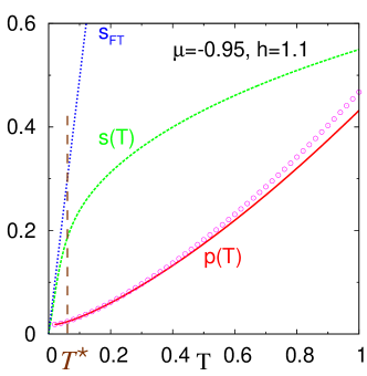
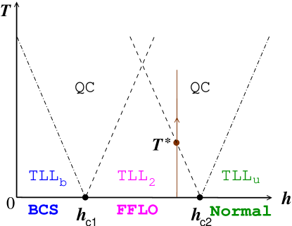
Figure 1: (Color online) Left panel: Comparison of the temperature dependence of the pressure $p$ obtained by numerically solving the full TBA equations (circles) and simplified Eqs. (4)–(7) (solid line). The entropy $s(T)$ (green dashed line) is linear in $T$ at low temperatures, agreeing well with $s_{FT}$ (blue dotted line) as predicted by the low energy effective field theory. $\mu=-0.95$ and $h=1.1$. The energy and length units are $\varepsilon_{B}/2$ and $a_{1}$, respectively. Right panel: The schematic finite-temperature “phase diagram” in the regime Eq. (3).

In the low temperature limit $T\ll\mu_{b},\mu_{u}$ we calculate the free energy using a Sommerfeld expansion based on Eqs. (4)–(5). Indeed, we find the thermodynamic potential reproduces the field theory result [Eq. (2)] and the corresponding entropy (per unit length)

$$s_{FT}=\frac{\pi}{3\hbar}(\frac{1}{v_{b}}+\frac{1}{v_{u}})T+...\,.$$ (10)

The entropy $s(T)$ obtained from Eqs. (4)–(7) is shown in Fig. 1 together with the low energy effective field theory result $s_{FT}$. $s(T)$ is clearly linear in $T$ at low temperatures and agrees well with $s_{FT}$. The deviation from the linear $T$ dependence marks a universal crossover around $T^{*}$ from relativistic to non-relativistic dispersion for particle- and hole-like excitations. This leads to a minima in the magnetization as well as in the densities (not shown in Fig. 1) at roughly the same temperature scale $T^{*}$. Analogous crossover phenomena were discussed in the magnetization curve for gapped spin-1 Heisenberg chains Maeda et al. (2007) and experimentally observed in two-leg spin ladders Rüegg et al. (2008).

The gross features of our findings are summarized in the schematic “phase diagram” in Fig. 1. There is no phase transition at finite temperature but only crossovers between different regimes. At low temperatures, the BCS, normal, and FFLO phase become the relativistic TLL of bound pairs (TLL_b), unpaired fermions (TLL_u), and two-component TLL (TLL₂) respectively. The TLL description of the FFLO phase breaks down at crossover temperature $T^{*}$ where the dispersion of either bound pairs or leftover fermions becomes non-relativistic. In particular, in the vicinity of the quantum critical points ($h_{c1}$ and $h_{c2}$), the system crosses over to the “quantum critical (QC) regime”. The other crossover (dash-dot) lines roughly correspond to the excitation gap for unpaired fermions or bound pairs.

Application: two-stage thermometry. Now we use these formulas to study the strongly interacting imbalanced Fermi gas inside a 1D harmonic trap of frequency $\omega$. According to the local density approximation, the chemical potential varies in space as $\mu(x)=\mu_{0}-\frac{1}{2}m\omega^{2}x^{2}$, with $x=0$ corresponding to the center of the trap, while the magnetic field $h$ stays constant. Thus, distinct zero temperature phases are realized at different locations in the trap, giving rise to particular spatial structures in the in-situ density images. A central challenge in interpreting the density distribution data from experiments is how to determine ($T,\mu_{0},h$), none of which seems to be accurately measurable so far.

We use our results to propose a two-stage scheme to accurately determine the parameters $T$, $\mu_{0}$, and $h$ from the density profiles. Stage 1: estimate the values of these parameters using the density profiles at the phase boundary and at the edge of the gas cloud. Stage 2: using the estimations as guess inputs, obtain ($T,\mu_{0},h$) to high accuracy by a direct three-parameter fit of the whole density profile using Eq. (9). Previously, thermal tails at the outer wing of the density cloud have been used to extract the temperature of atomic gases in 3D traps based on the observation that the gas is essentially non-interacting there Shin et al. (2008); Ho and Zhou (2009). Here, by contrast, the outer wing may still interact strongly (e.g., it might be a Tonks-Girardeau gas). Moreover, our method utilizes densities not only at the edge of the cloud, but also at the interface. We now illustrate how to accomplish the goals of Stage 1 for the cases of low and high total polarization.

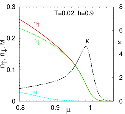
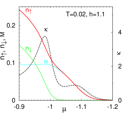
Figure 2: The density $n_{\uparrow}$, $n_{\downarrow}$, the magnetization $M=n_{\uparrow}-n_{\downarrow}$, and the compressibility $\kappa=\partial n/\partial\mu$ versus the local chemical potential $\mu$ in a 1D trap. Left panel: low polarization, $h=0.9$. Right panel: high polarization, $h=1.1$. The temperature $T=0.02$ (units are the same as Fig. 1). $\kappa$ develops a peak at the thermal tail of the gas or at the phase boundary. Its peak value depends sensitively on temperature.

For low polarization, the trap consists of a partially polarized (FFLO) core and a fully paired (BCS) wing, which at strong coupling is a Tonks-Girardeau gas. Representative finite $T$ density distributions are shown in the left panel of Fig. 2. At $T=0$, the magnetization $M$ drops to zero at the FFLO-BCS phase boundary $\mu=-h+n^{3}\pi^{2}a_{1}/24$ Guan et al. (2007), while $n_{\uparrow}$ and $n_{\downarrow}$ vanish at $\mu=-\varepsilon_{B}/2$. Finite temperature leads to thermal tails for all three. The compressibility $\kappa$ is also shown in Fig. 2, which develops a peak near the edge of the cloud. At $T=0$, $\kappa$ diverges as $\sim 1/\sqrt{\mu+\varepsilon_{B}/2}$ as $\mu$ approaches $-\varepsilon_{B}/2$. At finite temperature, this divergence is replaced by a peak which is increasingly shifted away from $\mu=-\varepsilon_{B}/2$ and becomes less pronounced as the temperature is raised. In the BCS region, $p_{u}$ is essentially zero, and the equation of density [Eq. (9)] simplifies to $n=4\alpha/(1+a_{1}\alpha)$. An analytic formula for $\kappa$ follows with its peak value given by the simple expression

$$\kappa_{\mathrm{pk}}=0.712[\sqrt{\frac{2m}{\hbar^{2}T}}-\frac{1.29}{\epsilon_{B}a_{1}}+\ldots].$$ (11)

For strong interaction and low temperatures, the second and higher order terms can be neglected. This formula provides a powerful way to estimate $T$, namely the peak of compressibility is a sensitive thermometer. In fact, $T$, $\mu_{0}$, and $h$ can be determined from experimentally measured $n(x)$ and $M(x)$, in the following steps. (A) Obtain the profile of compressibility from the density distribution in the trap, $\kappa(x)=-(m\omega^{2}x)^{-1}\partial n/\partial x$. (B) Read off the position, $x_{\mathrm{pk}}$, and the magnitude of the compressibility peak, $\kappa_{\mathrm{pk}}$, from the plot $\kappa(x)$. (C) Calculate $T$ from $\kappa_{\mathrm{pk}}$, using Eq. (11). (D) Estimate the value of the chemical potential $\mu_{0}$ at the center of the trap from $\mu_{b}(x_{\mathrm{pk}})=\mu_{0}-m\omega^{2}x^{2}_{\mathrm{pk}}/2+\varepsilon_{B}/2\simeq 0.554T$. (E) Estimate $h$ using $h=-\mu_{0}+m\omega^{2}x_{M}^{2}/2$, where $x_{M}$ is read off from the magnetization profile $M(x)$ at the value of $M(x_{M})=0.605\sqrt{mT/2\pi\hbar^{2}}$. Note that the thermal tail of $M$ is usually very broad, because $\mu_{u}\ll\mu_{b}$ is typically smaller than $T$ for low polarization.

For high polarization, a typical finite $T$ density profile is shown in the right panel of Fig. 2. At zero temperature, the trap consists of a partially polarized (FFLO) core and fully polarized normal (N) wing, with $n_{\downarrow}$ decaying to zero at the FFLO-N phase boundary. Thermal fluctuations smear the $T=0$ phase boundary, but the compressibility develops a pronounced peak at $x=x_{p1}$ due to the rapid decay of $n_{\downarrow}$ at low temperatures. In the normal region at the outer wing, the fully polarized gas is free and we found that the compressibility has the simple form $\kappa=-(m/2\pi\hbar^{2}T)^{1/2}\mathrm{Li}_{-1/2}(-e^{\mu_{u}/T})$. In this region, the thermal tail of $n_{\uparrow}$ leads to a second peak in the compressibility at $x=x_{p2}$. The two-peak structure of the compressibility is clearly seen in Fig. 2. The first stage estimation of ($T,\mu_{0},h$) in this case involves three steps. (A’) Measure the value of compressibility, $\kappa_{p2}$, at the second (outer) peak, and obtain the temperature from the relation $$\kappa_{p2}=0.126\sqrt{\frac{2m}{\hbar^{2}T}}.$$ (12) (B’) Estimate $\mu_{0}$ from the first (inner) peak location $x_{p1}$, using $\mu_{b}(x_{p1})=\mu_{0}-m\omega^{2}x^{2}_{p1}/2+\varepsilon_{B}/2\simeq 0.554T$. (C’) Estimate $h$ from the second peak location $x=x_{p2}$ using $\mu_{u}(x_{p2})=\mu_{0}-m\omega^{2}x^{2}_{p2}+h=1.11T$.

The authors thank Carlos Bolech, Jason Ho, Randy Hulet, and Qi Zhou for helpful discussions. The work is supported by the DARPA OLE Program and ARO (EZ and WVL), the Australian Research Council (XWG and MTB), and MEXT of Japan (MO).

References

- Zwierlein et al. (2006) M. W. Zwierlein, A. Schirotzek, C. H. Schunck, and W. Ketterle, Science 311, 492 (2006).
- Partridge et al. (2006) G. B. Partridge, W. Li, R. I. Kamar, Y.-A. Liao, and R. G. Hulet, Science 311, 503 (2006).
- Parish et al. (2007a) M. M. Parish, F. M. Marchetti, A. Lamacraft, and B. D. Simons, Nat. Phys. 3, 124 (2007a).
- Parish et al. (2007b) M. M. Parish, S. K. Baur, E. J. Mueller, and D. A. Huse, Phys. Rev. Lett. 99, 250403 (2007b).
- Zhao and Liu (2008) E. Zhao and W. V. Liu, Phys. Rev. A 78, 063605 (2008).
- Yang (2001) K. Yang, Phys. Rev. B 63, 140511 (2001).
- Moritz et al. (2005) H. Moritz et al., Phys. Rev. Lett. 94, 210401 (2005).
- Hulet (2009) R. G. Hulet (2009), private communications.
- Takahashi (1999) M. Takahashi, Thermodynamics of One-Dimensional Solvable Models (Cambridge University Press, Cambridge, 1999).
- Kakashvili and Bolech (2009) P. Kakashvili and C. J. Bolech, Phys. Rev. A 79, 041603 (2009).
- Casula et al. (2008) M. Casula, D. M. Ceperley, and E. J. Mueller, Phys. Rev. A 78, 033607 (2008).
- Gaudin (1967) M. Gaudin, Phys. Lett. A 24, 55 (1967).
- Yang (1967) C. N. Yang, Phys. Rev. Lett. 19, 1312 (1967).
- Orso (2007) G. Orso, Phys. Rev. Lett. 98, 070402 (2007).
- Hu et al. (2007) H. Hu, X.-J. Liu, and P. D. Drummond, Phys. Rev. Lett. 98, 070403 (2007).
- Guan et al. (2007) X. W. Guan, M. T. Batchelor, C. Lee, and M. Bortz, Phys. Rev. B 76, 085120 (2007).
- Blöte et al. (1986) H. W. J. Blöte, J. L. Cardy, and M. P. Nightingale, Phys. Rev. Lett. 56, 742 (1986).
- Affleck (1986) I. Affleck, Phys. Rev. Lett. 56, 746 (1986).
- Maeda et al. (2007) Y. Maeda, C. Hotta, and M. Oshikawa, Phys. Rev. Lett. 99, 057205 (2007).
- Rüegg et al. (2008) C. Rüegg et al., Phys. Rev. Lett. 101, 247202 (2008).
- Shin et al. (2008) Y.-I. Shin, C. H. Schunck, A. Schirotzek, and W. Ketterle, Nature 451, 689 (2008).
- Ho and Zhou (2009) T.-L. Ho and Q. Zhou (2009), arXiv:0901.0018.