Quantifying Spectral Features of Type Ia Supernovae

Abstract

We introduce a new technique to quantify highly structured spectra for which the definition of continua or spectral features in the observed flux spectra is difficult. The method employs wavelet transformation which allows the decomposition of the observed spectra into different scales. A procedure is formulated to define the strength of spectral features so that the measured spectral indices are independent of the flux levels and are insensitive to the definition of continuum and also to reddening. This technique is applied to Type Ia supernovae spectra, where correlations are revealed between the luminosity and spectral features. The current technique may allow for luminosity corrections based on spectral features in the use of Type Ia supernovae as cosmological probe.

1 Introduction

A major difficulty in analyzing spectroscopic data with highly blended atomic lines is to quantify the strength of certain spectral features. These spectral features are superimposed on a continuum so line blending can make it difficult to reliably define the continuum level. In the case of supernova spectra, the pre-nebular phase spectra typically show P-Cygni profiles with both emission and absorption components whereas the nebular phase spectra are dominated by broad overlapping emission lines. The spectral features are therefore of various widths and strengths, and neighboring features are heavily blended. Further, the data typically contain observational noise, flux calibrations errors and uncertainties in the amount of dust extinction. The noise makes the definition of a continuum very uncertain and accordingly the calculation of equivalent width becomes unreliable. In many observations, in particular those at high redshift, the observed supernova spectra are heavily contaminated by host galaxy spectra. This affects severely the definition of line depth.

For Type Ia supernovae, it is known that certain spectral line ratios such as the Si II 5800/Si II 6150, and the Ca II H&K lines are sensitive to the intrinsic brightness of the supernova Nugent et al. (1995). The measurement of the line strength is, however, not trivial. For instance, to measure the Si II 5800/Si II 6150, and the Ca II ratio, Nugent et al. (1995) employed a simple approach by drawing straight lines at the local peaks of the spectral features and measure the depth of the absorption minima from the straight line. However, the location of the straight line and the position of the line minimum are not easy to define in the presence of observational errors. It is for this reason the ratio is derived only for a number of very well observed local supernovae.

In this paper, the spectral features of Type Ia supernovae will be analyzed instead through wavelet transformations. This technique avoids many of the challenges mentioned above associated with identifying line strengths. Here wavelet transformations are applied to Type Ia supernovae spectra with the purpose to quantify the spectral features for cosmological applications.

Figure 1: (a) The spectrum of SN 2001el, (b-j) the wavelet scales 1 to 9, and (k) the smoothed array $c_{p}$ of the SN 2001el from top left to lower right. A sum of of scales (b) to (k) recovers the original spectrum (a). The mean fluxes of each of the wavelet scales (b) to (j) are identically zero.

2 Spectral Features

2.1 Wavelet Transform Algorithm

It has been previously demonstrated that the à trous algorithm Holtschneider et al. (1989); Starck et al. (1995, 1997) is a very useful tool for studying spectral features. The transform is carried out in direct space so artifacts related to periodicity do not occur. The reconstruction is trivial. The evolution of the transform from one scale to the next is easy to follow and the interpretation of the spectrum at each scale is straightforward.

The à trous wavelet uses a dyadic wavelet to merge non-dyadic data in a simple and efficient procedure. Assuming a scaling function $\phi(x)$ (which corresponds to a low pass filter), the first filtering is performed on the original data $\{c_{0}(k)\}$ by a twice magnified scale leading to the $\{c_{1}(k)\}$ set. The signal difference $\{c_{0}(k)\}-\{c_{1}(k)\}$ contains the information between these two scales and is the discrete set associated with the wavelet transform corresponding to $\phi(x)$. The operation is performed successively and to obtain the wavelet scale $w_{j}(k)$ at each scale $j$. The original spectrum $c_{0}$ can be expressed as the sum of all the wavelet scales and the last smoothed array $c_{p}$:

$$c_{0}(k)\ =\ c_{p}(k)\ +\ \Sigma^{p}_{j=1}w_{j}(k)$$

To demonstrate the basic features of the à trous wavelet transformation, we show in Figure 1 the wavelet transformation of a well observed supernova SN 2001el. The data were obtained through the spectropolarimetry program at the Very Large Telescope of the European Southern Observatory Wang et al. (2003). The sampling step of the data is binned to 5Å. The signal to noise ratio (SNR) of the data is everywhere above 150 - this unusually high SNR is a result of the spectropolarimetry observations. The original data is show in Figure 1a, and the consecutive wavelet scales for j = 1, 9 are shown in Figure 1b to 1j. Figure 1k represents the smoothed array $c_{p}$: given the spectral range of SN 2001el the à trous wavelet cannot generate more than 10 wavelet scales. Further note that each of the individual wavelet scales have zero mean. It can be seen that at small scales the wavelet is dominated by observational noise and the supernova signal starts to become significant only for $j\geq 3$, and the broad spectral wiggles associated with the supernova dominate the wavelet scales of j = 5, 6, and 7. The supernova spectral features are typically a few hundred Å wide and are effectively isolated in the decomposed spectra.

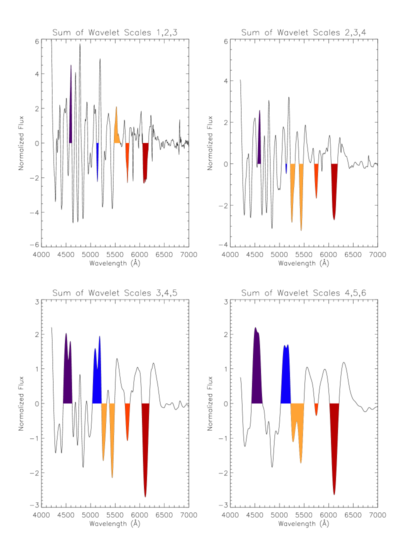
The spectral features of a supernova can be better described by a blend of several wavelet scales. For this reason, we can calculate the sum of more than one scales to reflect the existence of features of various width:

$$W_{\{l\}}\ =\ \Sigma_{j\in{\{l\}}}w_{j},$$

where $\{l\}$ is a subset of wavelet scales. Examples of these spectra are shown in Figure 2 for SN 2001el.

Figure 2: Wavelet sums for SN 2001el over (a) scales 1 to 3, (b) 2 to 4, (c) 3 to 5, (d) 4 to 6, (e) 5 to 7, (f) 6 to 8 and (g) 7 to 9. Running combinations of the different scales captures features of varying width.

2.2 Normalization of Spectral Features

The wavelet scales, having the units of the original flux spectrum, need to be normalized to construct quantities that measure the strength of the spectral features that do not depend on the absolute flux level of the spectrum. There undoubtedly is more than one way to normalize the scales. The simplest approach is to normalize all the wavelet scales by dividing them by the smoothed array $c_{p}$. This approach is simple and will certainly work fine for data without host galaxy contamination. For data with host galaxy contamination, or those with poor background subtraction, this approach introduces systematic errors to the normalized scales.

In our approach, the normalized wavelet scale is defined using the standard deviations of the spectral features from any given wavelet scale:

$${\hat{W}_{\{l\}}}(\lambda)\ = \ W_{\{l\}}(\lambda)/\sqrt{\Sigma_{\lambda_{1}}^{\lambda_{2}}W_{\{l\}}^{2}(\lambda)/N_{12}}$$ (1)

$$= W_{\{l\}}(\lambda)/\sigma_{\{l\}},$$ (2)

where $N_{12}$ is the number of data points between $\lambda_{1}$ and $\lambda_{2}$. The mean and standard deviation of ${\hat{W}_{\{l\}}}$ are zero and 1, respectively. This is effectively a self-normalization that exploits only the intrinsic properties of the wavelet scales involved. Host galaxy contamination (which does strongly affect $c_{p}$) would not have a significant effect in this context.

The spectral index $X_{j}$ of any feature between $\lambda_{a}$ and $\lambda_{b}$ at a given scale $j$ is defined by averaging the normalized wavelet scale $\hat{W}_{j}$:

$$X_{\{l\}}\ =\ \Sigma_{\lambda_{a}}^{\lambda_{b}}\hat{W}_{\{l\}}(\lambda)/N_{ab},$$

with $N_{ab}$ being the bin size in the wavelength region $\lambda_{a}$ and $\lambda_{b}$. $X_{j}$ defines a normalized number which measures the strength of the spectral features in the normalized wavelet scale $\hat{W}_{j}$ between $\lambda_{a}$ and $\lambda_{b}$. Alternatively, one can also calculate the power $P_{j}$ between $\lambda_{a}$ and $\lambda_{b}$ for wavelet scale $j$:

$$P_{\{l\}}\ =\ \Sigma_{\lambda_{a}}^{\lambda_{b}}\hat{W}_{\{l\}}^{2}(\lambda)/N_{ab}.$$

$P_{\{l\}}$ and $X_{\{l\}}$ contain the same information. In this study, we will focus on $X_{\{l\}}$.

One obvious advantage to using wavelet scales to estimate spectral feature strengths is that they do not depend on the definition of the spectral continua. Furthermore, since they can be estimated locally around a spectral feature, spectral indices are useful in minimizing uncertainties due to errors in spectral flux calibrations. Similarly, the spectral indices as defined here are less sensitive to errors of background subtraction, which is usually one of the dominate sources of uncertainty, especially in the studies of high redshift supernovae.

2.3 Normalization Spectral Features of SN Ia

The wavelet technique is particularly well-suited for studying scattering-dominated spectra of expanding atmospheres with P-Cygni spectral features: the net flux of the P-Cygni feature is usually close to zero. Wavelet decomposition is consistent with this as the mean flux is zero for the various wavelet scales. Wavelet transforms thus makes it easy to separate emission and absorption components of a spectrum in a mathematically robust way.

In this study, the supernova spectra are first decomposed into various scales as described in the above section. In addition, to reflect the fact the spectral features are a blend of different scales, the sum of the wavelet scales 3, 4, and 5 are used as the primary spectrum for the analysis of spectral features (though other scales have also been analyzed). All the decomposed spectra are normalized in a similar way as given in Equation 2. To derive quantities that are less sensitive to errors of flux calibration, we need to restrict calculation of the normalization factor to a small wavelength region and yet to have large enough spectral coverage so that the feature strengths will not be affected by boundary. In this study, the spectra are divided into four regions: (A) 5500 to 6500 Å, (B) 4985 to 5985 Å, (C) 4850 to 5450 Å, and (D) 4250 to 5200 Å; the variance in each of these sections of spectra is calculated and used as the normalization factor. Interesting features include the Silicon II lines at 635.5 and 580.0 nm in region (A), the Silicon II line around 548.5nm in region (B), and the two strong peaks at 510.0 nm and 450.0 nm, in region (C) and (D), respectively. These five spectral features are shown in Figure 3 and are the main focus of subsequent analyses.

Figure 3: Spectral features for Type Ia supernovae. (a): l = 1,2,3. (b): l = 2,3,4, (c) l = 3,4,5, and (d) l = 4,5,6. The spectral features are well resolved in (c) and (d).

3 Biases and Errors

In practice, the observed data contain noise and estimates of $X_{j}$ can be biased. The noise affects $X_{j}$ in two ways: First, when the noise is large, its effect can propagate to all the wavelet scales and become a significant component at the wavelet scale of interest. Secondly, it changes the normalization factor when calculating $\hat{W}_{j}$ - data with larger noise can be systematically biased to give a larger normalization factor because the additional power from shot noise. This bias is usually not a problem for high SNR ratio data, but can be significant for data with a low SNR ratio. The correction factor $\Pi(j)$ for scale j is defined as:

$$\sigma_{0}(j)\ =\sigma(j)\Pi_{1j},$$ (3)

where $\sigma_{0}(j)$ is the variance at the jth scale in the ideal case of no photon shot noise.

Typically, published spectroscopic data do not have associated noise spectra. One instead has to rely on the flux spectrum to estimate the noise levels. A major advantage of wavelet transformation is that it allows estimates of the noise characteristics based on the spectral data itself. If we assume that all the continuum or spectral features are much broader than the data sampling step, the spectral fluctuations of the wavelet scale with $j=1$ should then represent mostly shot noise. This is generally reasonable as can be seen in Figure 1 (b) for the spectrum of Type Ia supernova 2001el.

Recognizing that smaller wavelet scales contain more information of the noise property than larger wavelet scales, we can define the spectral quality index (SQI) of the normalized wavelet scale $\{l\}$ as the variance ratio of normalized scale $\{l\}$ and the lowest normalized scale $\{1\}$:

$$\rho_{{\{l\}}\{1\}}\ =\ \Sigma_{\lambda 1}^{\lambda 2}\hat{W}_{\{l\}}^{2}/\Sigma_{\lambda 1}^{\lambda 2}\hat{W}_{\{1\}}^{2},$$ (4)

where the braces $\{\}$ reflect that the various quantities are actually sums of various wavelet scales. Specifically, $\hat{W}_{\{1\}}$ is the normalized sum of three wavelet scales, where $\{l\}$  =  1,2,3 in this instance. The SQI measures the relative importance of noise levels in estimating of the spectral feature index. It can be calculated directly from the decomposed spectra without an error spectrum. Note that SQI is a quantity that can be localized to certain wavelength intervals.

For a given spectrum {$c_{i}$}, the dependence of the wavelet spectral indices $X_{\{l\}}$ and the correction factor $\Pi$ on SQI can be estimated through Monte-Carlo simulations.

3.1 Dependence of Spectral Features on Observational Noise

Monte Carlo simulations are required to quantify the dependence of $X$ indices on observational noise. The characteristic parameter of the noise is the SQI defined in Equation 4 - the ratio of spectral variance of combined wavelet scales ${l}\ =\ {3,4,5}$ to that of the combined scales ${l}\ =\ {1,2,3}$. To perform such these simulations one needs a series of noise free spectra of supernova spectra. The spectropolarimetry program at the ESO VLT has acquired several high quality spectra of SN Ia with SNR ratios around 150 (2003ApJ…591.1110W). Spectra of SN 2001V and SN 2001el from the spectropolarimetry program will be used in this simulation to quantify the relations between $X$ and SQI.

In the example shown in Figure 4, various levels of Poisson noises were added to the spectrum of SN 2001el at day +1. The noise is added to the spectra, which are then transformed to various wavelet scales and the various $X$ indices are calculated. The top panel in Figure 4 shows the relation between $\rho$ and the assumed SNR ratio with the addition of Poisson noise. The SQI is calculated in the wavelength intervals of 550.0 nm to 650.0 nm, 498.5nm to 598.5 nm, and 425.0 to 520.0 nm. It can be seen that $\rho$ is correlates well with the SNR ratio of the input data: reducing the SNR ratio decreases $\rho$. This confirms that the SQI can effectively capture effect the photon shot noise, and can be used to quantify the noise level of the data.

The variances used to normalized the spectra at the various wavelet scales are clearly correlated. This is shown in the middle panel of Figure 4, where the data exhibit nearly identical slopes over the different wavelength regions. A linear relationship between $\sigma^{2}(1)$ and $\sigma^{2}(3)$, and between $\sigma^{2}(1)$ and $\sigma^{2}(4)$ is assumed for the fits. The slopes $\gamma_{1j}$ extracted from these fits are given in Table 1.

Figure 4: (Top) The relation between the SQI and the input SNR ratios. The solid lines show SQI of fourth wavelet scale and the dashed line the third. (Middle) The relation between the variance of the third and first wavelet scales. The effect of a large $\sigma(1)$ propagates linearly to larger wavelet scales. (Bottom) The correlation of the bias correction factor and SQI for the third wavelet scale. The SNR was varied in all cases via the addition of noise in the Monte Carlo simulations.

The bottom panel in Figure 4 clearly demonstrates how the correction factor $\Pi$ increases dramatically for $\rho$ approaching 2.82 (which corresponds to a SNR ratio of below 1 per 0.5 nm bin). This implies that the spectral features are dominated by the noise, hence it becomes impossible to extract the spectral indices reliably.

The correction factor for $\rho$ can be fit well with a function

$$\Pi_{1j}\ =\ \sqrt{(1-\gamma_{1j}\rho_{1j}^{2})},$$ (5)

with the relevant coefficients taken from Table 2 for the various lines.

3.2 Bias corrections

The various $X$ indices for the spectral features are derived from the Monte-Carlo simulation of data with different SQI. As shown in Figure 5, the $X$ indices (shown as open squares apparently suffer strong bias when the data are noisy. The various $X$ indices after $\Pi$ corrections are shown in Figure 5. The effect is generally small for high SNR ratio data, but becomes important for data with low SNR ratio. In any case the bias is effectively removed by applying the correction factor $\Pi$.

Figure 5: Line indices corrected for $\rho$ dependence for important SN Type 1a spectral features. The $X$ indices are derived from the sum of of wavelets 3,4,5 of SN 2001el 1 day past optical maximum.

3.3 Error Estimates of the Spectral Indices

Assuming photon shot noise, the Monte Carlo simulations also give error estimates for the $X$ indices. The errors as a function of $\rho$ are shown in Figure 6. These errors are fitted with a function of the form:

$$\sigma_{X}\ =\ {\eta\rho^{\psi}},$$ (6)

and the relevant coefficients $\eta$ and $\psi$ are shown in Table 2. Simulations were performed for all of the SN 2001V and SN 2001el spectra and it was found that in all cases the bias can be well corrected. Note that due to the lack of a completely noise-free SN Ia spectrum, at extremely high SNR ratio (such as those that are higher than or comparable with the signal to noise ratio of the SN 2001el spectra as used in the simulation) the Monte Carlo simulations do not give correct estimates of the errors. Such cases are unlikely to be relevant as in such situations, the errors are likely to be dominated by calibration systematics rather than shot noise. The error function given above will be used for all cases here. As can be seen in Figure 6, the above expression gives an excellent description of the dependence when the errors are described by $\rho$.

Figure 6: Errors of the $X$ indices as functions of $\rho$ for SN 2001el at optical maximum.

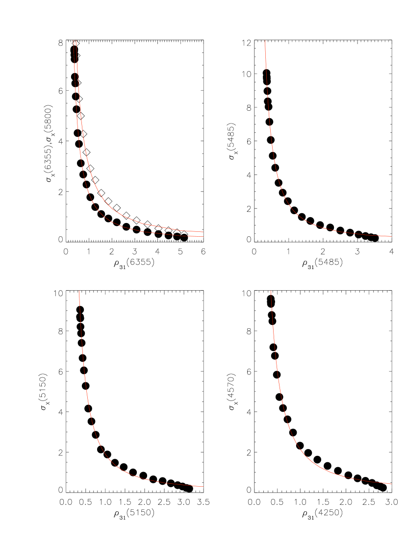
The $\rho$ dependence of the $X$ indices and their errors have a weak dependence among the different varieties of supernovae and the epoch of the supernovae.

Table 1: The Coefficients for the Dependence of $X$ on Data Errors

SN	Day	$\gamma_{31}(A)$	$\gamma_{31}(B)$	$\gamma_{31}(C)$	$\gamma_{31}(D)$	mean	$\gamma_{41}(A)$	$\gamma_{41}(B)$	$\gamma_{41}(C)$	$\gamma_{41}(D)$	mean
01V	$-8$	0.1132	0.1116	0.1183	0.1144	0.1144	0.0263	0.0240	0.0273	0.0259	0.0258
01el	$-4$	0.1220	0.1236	0.1229	0.1224	0.1227	0.0567	0.0587	0.0566	0.0573	0.0573
01el	+1	0.1220	0.1236	0.1229	0.1224	0.1227	0.0581	0.0583	0.0552	0.0551	0.0567
01el	+9	0.1251	0.1273	0.1250	0.1240	0.1254	0.0585	0.0607	0.0599	0.0577	0.0592

Table 2: The Coefficients for the Errors of $X$

SN	Date	$\eta(6150)$	$\psi(6150)$	$\eta(5800)$	$\psi(5800)$	$\eta(5485)$	$\psi(5485)$	$\eta(5150)$	$\psi(5150)$	$\eta(4250)$	$\psi(4250)$
2001V	$-8$	-0.02486	0.0469	-0.0156	0.0293	-0.0203	0.0601	-0.0373	0.0545	-0.0179	0.0453
2001el	$-4$	-0.00625	0. 0367	-0.00628	0.05429	-0.02449	0.05892	-0.01626	0.06382	-0.01165	0.05248
2001el	+1	0.133	1.248	0.212	1.188	0.160	1.412	0.176	1.533	0.157	1.531
2001el	+9	0.159	1.276	0.194	1.282	0.234	1.279	0.203	1.442	0.177	1.672
2001el	+1	0.145	1.194	0.265	1.322	0.175	1.295	0.181	1.500	0.216	1.408

Procedure for Bias and Error Estimation
The procedure for removing bias and estimating errors from noisy supernovae spectra is premised on extracting correction factors from a supernova with a large SNR. Here we enumerate a correction recipe using wavelet scales $l={3,4,5}$ with SN 2001 el as our reference spectrum.

1. Compute the ratio of the sum of the squares of wavelet scales 3,4,5 and 1,2,3 ($\rho_{31}$ in Eq. 4) for SN 2001 el

   $$\rho_{31}=\frac{\hat{W}^{2}_{\{3,4,5\}}}{\hat{W}^{2}_{\{1,2,3\}}}.$$

2. Degrade the SNR ratio of SN 2001 el in multiple steps with the addition of Poisson noise. Compute $\sigma_{\{1,2,3\}}^{2}$ and $\sigma_{\{3,4,5\}}^{2}$ at each step.

3. Extract $\gamma_{31}$ by assuming a linear relationship between $\sigma_{\{1,2,3\}}^{2}$ and $\sigma_{\{3,4,5\}}^{2}$ (see middle panel of Figure 4).

   $$\sigma^{2}_{\{3,4,5\}}=\beta+\gamma_{31}*\sigma^{2}_{\{1,2,3\}},$$

   where $\sigma_{\{l\}}$ is defined in Eq. 2.

4. Repeat each of the above steps over all regions of interest to extract a mean value for $\gamma_{31}$. Equivalently, use the values for $\gamma_{31}$ by consulting Table 1.

5. Using equation 5, compute $\rho_{31}$ values for each SNe having typical values of the SNR ratio.

6. Compute the correction factor $\Pi_{31}$ using this value of $\rho_{31}$ and the value of $\gamma_{31}$ computed for SN 2001 el

   $$\Pi_{31}=\sqrt{1-\gamma_{31}\rho^{2}_{31}}.$$

7. The spectral index of any supernovae feature can be corrected for bias by dividing the uncorrected value by $\Pi_{31}$ as in Eq. 3.

   $$X_{corr}=\frac{X}{\Pi_{31}}.$$

8. The error bars are determined from the same set of simulations. With $\sigma_{X}$ defined as in Equation 6 construct the relationship

   $$log_{10}(\sigma_{X})=\eta+\psi log_{10}(\rho_{31}),$$

   where all quantities refer to a SNe with a large SNR ratio (e.g. SN 2001 el). Equivalently, use the values for $\gamma_{31}$ by consulting Table 2.

9. With these values $\eta$ and $\psi$ compute the variance in the spectral index for a SN with a typical value of SNR as

   $$\sigma_{X}=10^{\eta}\rho_{31}^{\psi}.$$

4 Applications to Type Ia Supernovae

Spectral indices lend themselves to a quantitative analysis of the temporal and magnitude evolution of the spectral lines. Nugent et al. (1995) measured the ratio of the depths of the Si II 6150 Å and 5750 Å features and established correlations with $\Delta m_{15}$. Other studies of these and other spectral features have adopted slightly more elaborate procedures based on equivalent Hachinger et al. (2006) and pseudo equivalent widths (EW) Folatelli (2003); Garavini et al. (2007); Altavilla et al. (2009); Branch et al. (2009) to study these and other absorption features. Recently, Arsenijevic et al. (2008); Stanishev et al. (2007) have used wavelets coupled with the pseudo-EW technique to study a Si II absorption feature. Emission features have received less attention than absorption features and usually involve a distinct procedure from the absorption features Nugent et al. (1995); Bongard et al. (2006). Recently, Bailey et al. (2009) described a variance of the above methods wherein absorption and emission features in a training set of spectra are studied to extract the optimal flux ratio to $\Delta m_{15}$ correlation. This ratio is then applied to correct the magnitudes of other supernovae within a validation set.

The wavelet technique developed here differs in several important respects from those described in the preceding paragraph. Our methodology is premised on the existence of one (or more) very high SNR spectra. Spectral line strengths are first extracted for this high SNR spectrum from a combination of intermediate wavelet scales. Excluding the lowest and highest reduces the effects of noise and the continuum, respectively. Working with wavelets from a high SNR spectrum allows corrections to be made to lower SNR spectra. Perhaps the most salient difference is that performing our analysis entirely in wavelet space permits us to avoid definition of the continuum (the mean of the wavelet scales is zero and integration is performed from one zero on the leading to the next zero on the trailing edge of a feature). Consequently, we are able to work directly with line strengths of the features themselves, not their ratios. Lastly, this technique permits absorption and emission lines to be treated democratically. It is our expectation that the wavelet method gives to a more robust measure of line strength. In Sections 4.2 and 4.3 we apply this technique to data described in the subsequent section.

4.1 Data Sample

The supernovae included in this study are given in Table 4.1. A large number of low-z spectra (z $<$ 0.1) were collected from libraries that are publicly available, such as the SUSPECT Supernova Database and the Center for Astrophysics Supernova Archive, as well as other SNe that are available in the literature. The spectra are corrected by the host galaxy redshift but no dust extinction correction is applied. The original wavelength coverages, step sizes and SNR ratios of these spectra are vastly different. In our analysis, all the spectra are first rebinned to 5 Å sampling step for convenience. After wavelet decomposition was performed the spectra were checked for edge effects that would distort calculations, the affected spectra were removed.

Table 3: The Spectroscopic Sample of SNe Ia

SNe	$\Delta m_{15}$	Branch Subtype	$X_{6150}$	$X_{5750}$	$X_{5485}$	$X_{5150}$	$X_{4570}$	Spectra Source
1981B	1.125(0.010)	BL	-56.645(0.157)	-10.339(0.298)	-48.941(0.245)	42.956(0.175)	43.306(0.184)	1
1983G	1.37(0.01)	$\cdots$	-59.818(0.649)	-13.890(3.411)	$\cdots$	49.532(0.483)	$\cdots$	2
1984A	1.294(0.063)	BL	-63.615(0.974)	-5.166(1.167)	-39.319(0.489)	45.827(0.573)	43.895(0.781)	3
1986G	1.643(0.022)	CL	-49.109(0.295)	-20.165(0.534)	-32.227(0.456)	40.231(0.386)	51.494(0.521)	4
1989B	1.262(0.017)	CL	-54.202(0.486)	-13.218(0.428)	-47.078(0.424)	41.870(0.216)	46.161(0.318)	5,6
1990N	1.138(0.024)	CN	-53.751(0.112)	-9.683(1.763)	$\cdots$	39.630(0.312)	$\cdots$	7,8
1991T	0.986(0.009)	SS	-52.505(0.274)	-2.976(0.499)	-29.806(0.829)	34.860(0.159)	21.783(0.474)	9,10,11
1991bg	1.857(0.125)	CL	-46.461(0.324)	-25.588(0.582)	-22.972(0.382)	24.081(0.436)	51.622(0.367)	12,13,14
1992A	1.320(0.015)	BL	-54.040(0.242)	-16.239(0.517)	-46.671(0.447)	41.067(0.300)	36.031(0.336)	15
1993H	1.70(0.10)	$\cdots$	-46.790(6.947)	-21.166(3.053)	-27.335(0.697)	35.324(0.093)	51.183(1.020)	16
1994D	1.558(0.013)	CN	-53.234(0.212)	-14.450(0.182)	-48.604(0.216)	37.600(0.114)	35.566(0.207)	17,18
1996X	1.299(0.009)	CN	-53.837(0.216)	-9.917(0.400)	-51.935(0.309)	41.193(0.271)	43.070(0.317)	19,20
1997bp	1.231(0.013)	$\cdots$	-64.847(1.884)	-3.015(1.935)	$\cdots$	42.951(0.729)	$\cdots$	21
1997br	1.141(0.021)	SS	-43.186(4.832)	-21.652(3.106)	$\cdots$	40.701(0.171)	$\cdots$	22
1997do	1.099(0.237)	BL	-57.978(0.878)	-11.934(0.186)	$\cdots$	43.880(0.995)	$\cdots$	23
1997dt	1.04(0.15)	CN	-56.255(0.148)	-8.051(0.475)	-50.003(0.632)	41.675(0.655)	47.482(0.538)	23
1998V	1.150(0.025)	CN	-52.756(0.285)	-10.737(0.517)	-47.976(0.406)	42.455(0.300)	35.278(0.390)	23
1998aq	1.185(0.008)	CN	-53.695(0.218)	-9.824(0.404)	-51.130(0.322)	39.259(0.262)	31.908(0.403)	23,24
1998bp	1.903(0.013)	CL	-45.839(0.215)	-28.182(0.399)	-33.504(0.312)	27.849(0.458)	48.179(0.449)	23
1998bu	1.014(0.008)	CN	-53.743(0.137)	-10.060(0.255)	-48.582(1.067)	40.477(0.177)	32.800(1.149)	23,25,26,27
1998de	1.881(0.066)	CL	-48.672(0.294)	-28.202(0.533)	-21.675(0.329)	38.392(0.564)	56.127(0.232)	23
1998dh	1.258(0.038)	BL	-55.895(0.209)	-10.240(0.388)	-47.762(0.285)	43.403(0.257)	45.766(0.205)	23
1998dm	0.983(0.339)	$\cdots$	-53.027(0.094)	-12.198(3.126)	$\cdots$	47.453(0.919)	$\cdots$	23
1998ec	1.074(0.028)	BL	-62.305(0.121)	-4.422(0.232)	-47.332(0.591)	43.144(0.037)	42.297(0.887)	23
1998eg	1.15(0.09)	CN	-53.627(0.317)	-11.681(0.570)	-52.964(0.531)	37.920(0.349)	39.311(0.394)	23
1998es	0.745(0.013)	SS	-52.360(0.668)	-4.399(0.549)	-45.227(0.306)	42.884(0.086)	31.574(0.194)	23
1999aa	0.811(0.014)	SS	-51.631(0.885)	-5.908(0.408)	-44.397(0.210)	43.020(0.087)	30.685(0.214)	23,28
1999ac	1.241(0.036)	SS	-56.123(0.280)	-9.354(0.509)	-44.465(0.327)	42.953(0.272)	44.159(0.183)	23,29
1999aw	0.814(0.018)	$\cdots$	-52.965(4.726)	-1.590(0.431)	$\cdots$	$\cdots$	$\cdots$	30
1999by	1.796(0.008)	CL	-46.242(0.484)	-27.599(0.338)	-23.743(0.369)	34.528(0.282)	56.148(0.363)	23
1999cc	1.567(0.102)	BL	-54.551(0.368)	-17.619(0.654)	-46.891(0.486)	40.408(0.439)	41.747(0.363)	23
1999cl	1.243(0.043)	BL	-59.260(0.397)	-6.847(0.703)	-38.325(0.538)	43.409(0.161)	46.195(0.193)	23
1999dq	0.973(0.030)	SS	-50.336(0.623)	-6.492(0.359)	-43.249(0.249)	43.592(0.086)	33.746(0.162)	23
1999ee	0.944(0.006)	SS	-52.461(0.418)	-9.313(0.737)	-48.746(0.446)	43.475(0.215)	39.278(0.177)	31
1999ej	1.446(0.018)	BL	-51.523(0.241)	-21.127(0.443)	-43.869(0.384)	36.897(0.338)	41.707(0.383)	23
1999gh	1.721(0.008)	BL	-53.856(2.065)	-21.929(0.901)	$\cdots$	39.822(3.692)	$\cdots$	23
1999gp	1.029(0.186)	SS	-54.055(0.844)	-3.634(1.409)	-46.510(0.863)	41.516(0.449)	37.941(0.408)	23
2000E	1.079(0.021)	SS	-51.938(0.250)	-7.507(0.493)	-46.913(0.479)	42.393(0.248)	33.210(0.667)	32
2000cf	1.364(0.043)	$\cdots$	-51.376(1.230)	-13.827(0.031)	-48.438(0.101)	41.395(0.424)	47.646(0.232)	23
2000cn	1.675(0.027)	CL	-51.405(0.250)	-23.634(0.078)	$\cdots$	38.841(1.773)	$\cdots$	23
2000cx	0.971(0.006)	SS	-52.441(0.429)	-4.527(0.755)	-41.327(0.525)	44.369(0.285)	29.687(0.418)	23,33
2000dk	1.457(0.033)	CL	-50.096(0.017)	-23.257(0.389)	-39.544(0.354)	34.195(0.406)	38.875(0.413)	23
2000fa	1.140(0.027)	CN	-54.210(0.551)	-9.293(1.827)	-44.606(1.594)	40.845(1.452)	33.094(1.348)	23
2001V	0.743(0.034)	SS	-52.006(1.813)	-5.376(2.106)	-35.152(3.846)	39.213(4.099)	29.718(0.170)	23
2001ay	0.543(0.006)	$\cdots$	-63.993(0.203)	-2.843(0.378)	-30.552(0.265)	39.397(0.309)	59.731(0.666)	34
2001el	1.166(0.004)	CN	-52.317(0.744)	-12.737(0.230)	-50.087(0.342)	40.832(0.272)	$\cdots$	35
2002bo	1.260(0.007)	BL	-61.527(0.322)	-5.877(0.821)	-41.535(0.730)	45.575(0.464)	41.272(0.458)	36
2002cx	1.145(0.016)	SS	-32.952(3.231)	-19.216(6.785)	-28.614(6.820)	20.330(2.847)	27.516(2.514)	37
2002dj	1.08(0.05)	$\cdots$	-63.346(0.267)	-2.519(2.441)	-46.720(0.321)	46.987(1.460)	38.889(0.614)	38
2002el	1.423(0.018)	$\cdots$	-54.749(0.349)	-15.368(0.904)	-45.108(0.855)	37.251(0.296)	37.339(0.567)	39
2002er	1.301(0.009)	BL	-56.853(0.227)	-10.436(0.420)	-49.949(0.369)	41.584(0.248)	45.197(0.332)	40
2003cg	1.25(0.05)	$\cdots$	-52.901(0.295)	-8.980(0.506)	-43.235(0.634)	38.695(0.223)	36.871(0.400)	41
2003du	1.151(0.037)	CN	-54.388(0.192)	-7.664(0.360)	-53.238(0.300)	40.229(0.287)	39.471(0.283)	42,43
2004S	1.210(0.016)	CN	-48.235(3.103)	-18.474(5.782)	$\cdots$	40.250(2.452)	$\cdots$	45
2004dt	1.299(0.002)	$\cdots$	-64.706(0.662)	-3.370(0.231)	-41.069(0.266)	34.912(0.214)	45.159(0.400)	46
2004eo	1.417(0.004)	CL	-49.673(1.001)	-20.883(0.351)	-40.903(0.220)	41.306(0.303)	49.330(4.384)	47
2005bl	1.93(0.10)	$\cdots$	-45.532(3.327)	-25.784(3.759)	-17.737(3.337)	27.149(0.361)	40.669(1.949)	48
2005cf	1.161(0.006)	CN	-52.758(0.249)	-11.505(0.457)	-52.686(0.316)	40.237(0.356)	43.805(0.364)	49
2005cg	0.942(0.048)	$\cdots$	-55.780(0.292)	-6.463(0.528)	$\cdots$	$\cdots$	$\cdots$	50
2005df	1.116(0.013)	$\cdots$	-53.024(0.064)	-9.486(3.441)	-51.371(0.514)	46.312(2.108)	37.292(2.676)	51
2005hj	0.743(0.165)	$\cdots$	-51.129(0.542)	-4.260(0.935)	-41.942(0.423)	49.066(0.336)	38.596(0.529)	52
2005hk	1.56(0.09)	SS	-42.299(6.056)	-27.804(1.861)	-16.555(1.580)	31.749(0.302)	30.752(14.932)	53
2006gz	0.69(0.04)	SS	-52.610(0.032)	-7.209(0.217)	$\cdots$	33.375(0.492)	$\cdots$	54
2006X	1.17(0.04)	BL	-66.111(0.252)	-0.616(0.195)	-25.726(0.209)	42.110(0.088)	38.500(0.186)	55

References. — (1) Branch et al. (1983); (2) Harris et al. (1983); (3) Barbon et al. (1989); (4) Phillips et al. (1987); (5) Barbon et al. (1990); (6) Wells et al. (1994); (7) Mazzali et al. (1993); (8) Leibundgut et al. (1991); (9) Filippenko et al. (1992a); (10) Phillips et al. (1992); (11) Ruiz-Lapuente et al. (1992); (12) Leibundgut et al. (1993); (13) Filippenko et al. (1992b); (14) Turatto et al. (1996); (15) Kirshner et al. (1993); (16) Wang unpublished; (17) Meikle et al. (1996); (18) Patat et al. (1996); (19) Wang et al. (1997); (20) Salvo et al. (2001); (21) Anupama (1997); (22) Li et al. (1999); (23) Matheson et al. (2008); (24) Branch et al. (2003); (25) Jha et al. (1999); (26) Meikle & Hernandez (2000); (27) Hernandez et al. (2000); (28) Garavini et al. (2004); (29) Garavini et al. (2005); (30) Strolger et al. (2002); (31) Hamuy et al. (2002); (32) Valentini et al. (2003); (33) Li et al. (2001); (34) Branch et al. (2006); (35) Wang et al. (2003); (36) Benetti et al. (2004); (37) Li et al. (2003); (38) Pignata et al. (2008); (39) Wang unpublished; (40) Kotak et al. (2005); (41) Elias-Rosa et al. (2006); (42) Anupama et al. (2005); (43) Stanishev et al. (2007); (44) Howell et al. (2006); (45) Krisciunas et al. (2007); (46) Altavilla et al. (2007); (47) Mazzali et al. (2008); (48) Taubenberger et al. (2008); (49) Garavini et al. (2007); (50) Quimby et al. (2006); (51) Quain in progress; (52) Quimby et al. (2007); (53) Phillips et al. (2007); (54) Hicken et al. (2007); (55) Wang et al. (2008)

4.2 $X$ Versus the Epochs

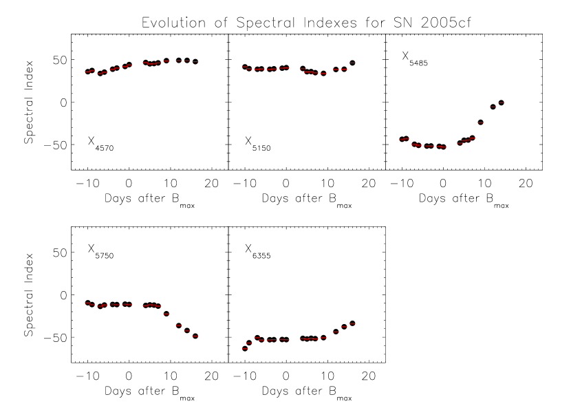
An example of the time evolution of $X$ indices is shown in Figure 7 for SN 2005cf - a normal Type Ia supernova with $\Delta m_{15}=1.16$. For a spectroscopically normal supernovae like SN 2005cf, the Si II 5800 and 6150 lines exhibit little evolution in line strength for roughly $\pm$8 days around maximum, after which the the 5800 Å line strengthens and the 6150 Å line weakens. Similarly, around 8 days past maximum the S II feature begins to weaken until it is completely obscured by 18 days past maximum. The emission features at 4750 and 5150 Å for this same supernova, by contrast, shows comparatively little time evolution.

Analysis of the time evolution is complicated by occasional large gaps between epochs and the need to occasionally track spectral features manually due to the decreasing velocity of the expanding photosphere. Consequently, a full analysis of the temporal evolution of the remaining supernovae in Table 4.1 will be analyzed in a separate paper.

Figure 7: The temporal evolution of the $X$ indices of SN 2005cf. In order these are: (a) the emission feature at 4570, (b) the emission feature at 5150, (c) S II line, (d)Si II 5800 line, (e) the Si II 6150.

4.3 $X$ versus $\Delta m_{15}$

Figures 8 to 12 show the correlations between $X$ and $\Delta m_{15}$ for the five spectral features that we have adopted for our study. The line strengths in these figures are those computed at maximum light. In instances where no spectrum at maximum light exists a simple quadratic fit was made of all spectra within 8 days of maximum (for features that are not a smoothly varying the fit was restricted to within 5 days of maximum). The fits were checked for consistency and for supernovae with only two spectra closely sampled in time, a mean was taken to avoid aberrant behavior in the fit. Any supernova having only a single spectrum within the specified time range was removed, unless that spectrum was taken at maximum.

4.3.1 The Si II 6150 Å line

Figure 8: The correlation of the strength of Si II 6150 feature and $\Delta m_{15}$.

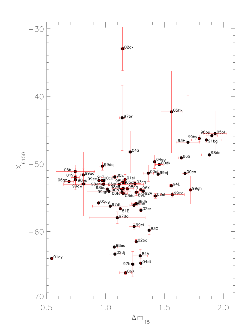
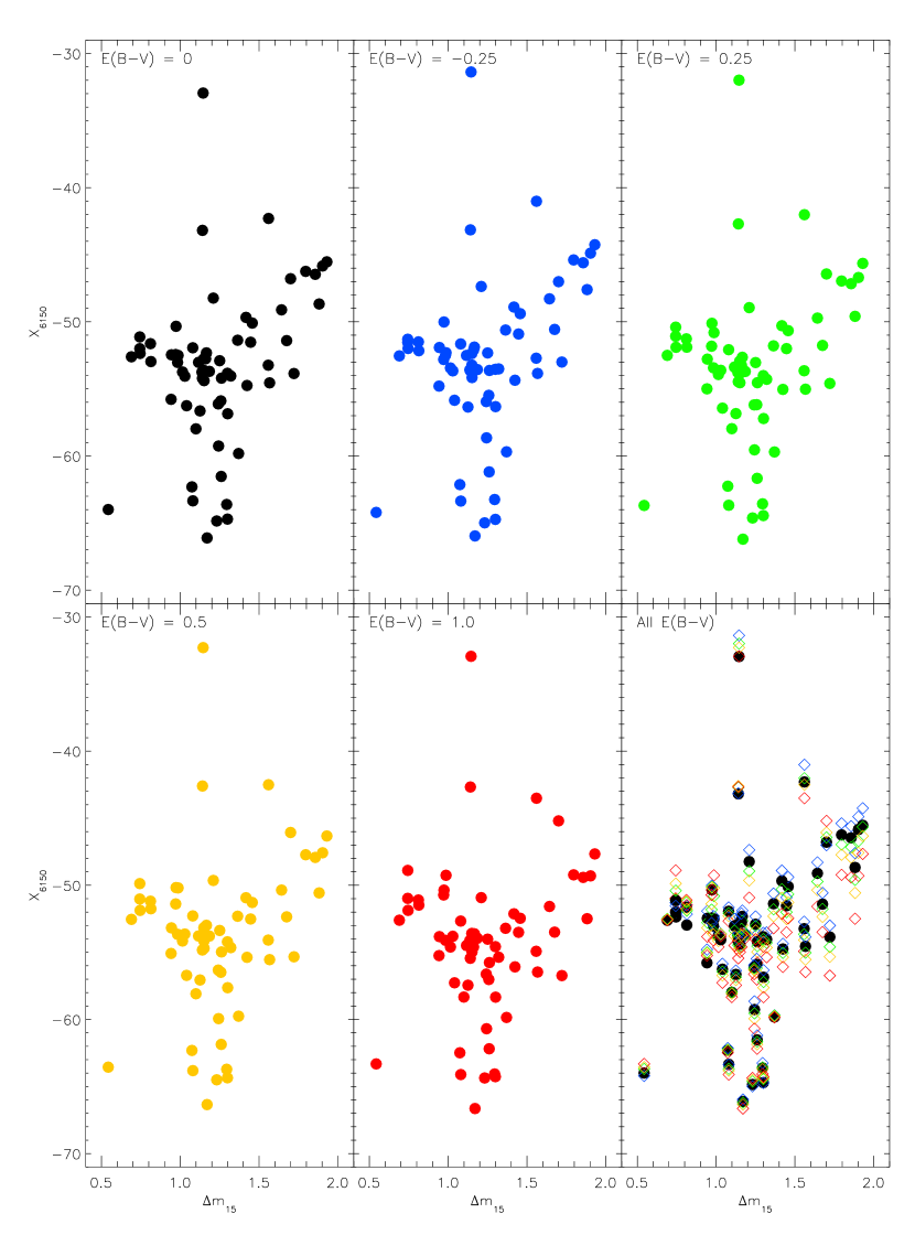
It has been shown previously that the strength of the Si II 6150 Å line is not tightly correlated with the intrinsic brightness Hachinger et al. (2006). Figure 8 confirms this observation in the main. However, the $X$ indices do show a modest trend of weaker spectral strength for dimmer supernovae and supernovae with $\Delta m_{15}$ less than 1 show large variations of the Si II 6150 strength. It merits mention that the several of these supernovae (e.g., SN 1997br, SN 2001ay, SN 2002cx, and SN 2005hk) are deviant with respect to the majority of the sample. It has been noted that these are all peculiar supernovae and it has been speculated that SN 1997br, SN 2002cx, and SN 2005hk may form a group distinct from most typical Type Ia supernovae Li et al. (1999, 2003); Branch et al. (2004); Howell & Nugent (2004); Branch et al. (2006); Jha et al. (2006); Phillips et al. (2007); Sahu et al. (2008); Branch et al. (2009).

4.3.2 Si II 5800 Å

Figure 9: The correlation of the strength of Si II 5800 and $\Delta m_{15}$.

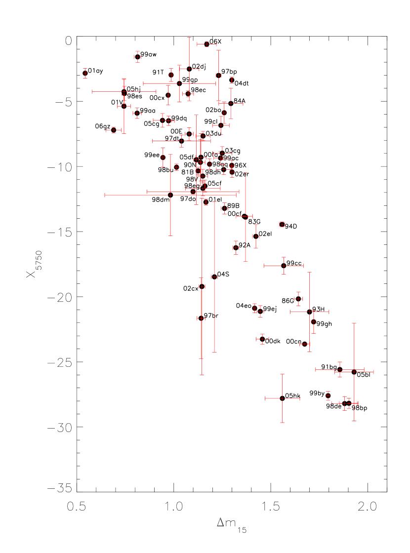
It has previously been shown that the ratio of the strength of this feature and that of the Si II 6150 Å line are well correlated with $\Delta m_{15}$ Nugent et al. (1995); Hachinger et al. (2006). Using this correlation, a determination of the supernovaes’ maximum luminosity may be determined on the basis of a single spectra Riess et al. (1998). These same two features have also been used to define Ia SNe subgroups Benetti et al. (2005); Branch et al. (2006, 2009).

Figure 9 shows the correlations with $\Delta m_{15}$. The $X$ index defined here for this line correlates tightly with $\Delta m_{15}$ even without having been divided by the strength of the Si II 6150 line. Note however, that the $X$ index for this feature is normalized by the total variance of the wavelength scales from wavelength region between 5500 Å and 6500 Å, the variations due to Si II 6150 Å line are partially included in the derivations of the $X$ indices. The correlation between $X$ and $\Delta m_{15}$ can be well described by a linear relation. It may be the case that for sub-luminous supernovae such as SN 1991bg, the feature 5800 Åmay actually be a blend of Ti II and Si II Garnavich et al. (2004) (although this has also been disputed Branch et al. (2006); Bongard et al. (2008)). Blending would artificially enhance the line strength and may suggest more of a correlation than in the absence of line blending. We wish to emphasize that the $X$ index of this feature measures the total strength of this feature and does not distinguish the physical origins of the features.

4.3.3 S II 5485

Figure 10: The correlation of the strength of S II 5485 and $\Delta m_{15}$.

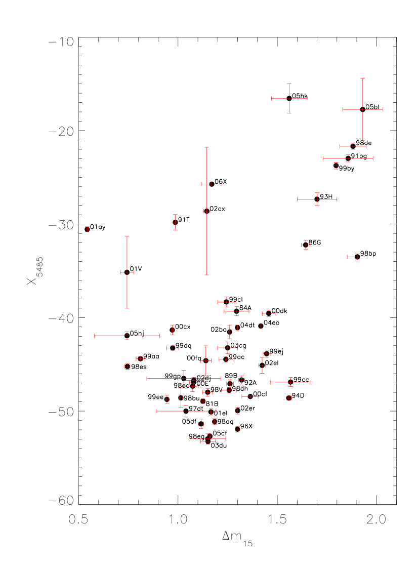
The “w” shaped spectral feature S II 5485 is another important line that defines an SN Ia similar to the Si II 6150 lines Bongard et al. (2006). Figure 10 suggests that the strength of this feature too may depend on $\Delta m_{15}$, though correlation is much weaker than that for Si II 5800. The deviant SNe are SN 1991T, SN 2001ay, SN 2005hk, SN 2006X, SN 2001V and SN 2002cx. SN 1997br has a similar spectral evolution to that of SN 1991T, but it has not been shown since it has only one spectrum within 5 days of maximum However the $X$ value ($-30$) for SN 1997br at 4 days before maximum is consistent with the $X$ value for SN 1991T. Other 1991T-like SNe (SN 1998es, SN 1999aa, SN 1999dq, SN 2000cx) have more normal values but they still are on the upper edge of the distribution. There is apparently some diversity within the so-called SN 1991T-like SNe.

The S II line is generally much stronger than the Si II 5800 line and is thus much easier to measure. There is also much more evolution within this feature so Figure 10 is restricted to spectra taken within 5 days of maximum.

4.4 5150 Emission Feature

Figure 11: The correlation of the emission peak at 5150 Å and $\Delta m_{15}$.

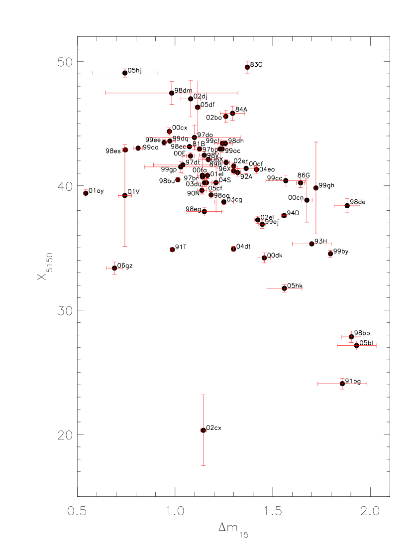
Figure 11 shows what might be interpreted as a slight dependence on $\Delta m_{15}$, though the trend is not as apparent as it is with the S II line. The $X$ values do decrease notably with $\Delta m_{15}$ for the most sub-luminous supernovae. A majority of the data are clustered with a large amount of scatter. The 5150 Å emission feature may not be a good indicator of decline rate.

4.5 4570 Emission Feature

Similar to Figure 11, Figure 12 shows what appears to be weak dependence on $\Delta m_{15}$ with the 4570 Å emission peak. As with Figures 9 and 10 the more deviant SNe appear on the outer edges of the distribution. This tendency is somewhat stronger than that found for the 5150 Å feature and is in the opposite direction: the $X$ value for 4570 Å is increasing with increasing $\Delta m_{15}$.

Figure 12: The correlation of the strength of the emission peak at 4570 Å and $\Delta m_{15}$.

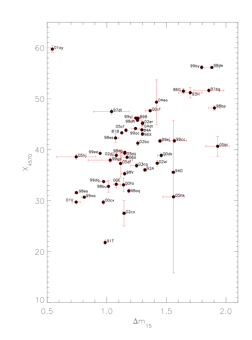
There is wide variation in early time evolution to this feature, so the data comprising Figure 12 is restricted to spectra taken within 5 days of maximum. Similar to the 5150 Å feature, the utility of the 4750 Å feature in specifying decline rate is uncertain.

4.6 Ratio Between the Emission Features at 4570 Å and 5150 Å 

The suggestion of a correlation between $\Delta m_{15}$ and the ratio of these two features appears in Figure 13, though it is also weak, particularly for the fast decliners. It appears that the 4570 Å feature has a stronger effect on this ratio than the 5150 Å feature.

Figure 13: The correlation of the ratio of the strength of the emission peak at 4570 Å and 5150 Å and $\Delta m_{15}$.

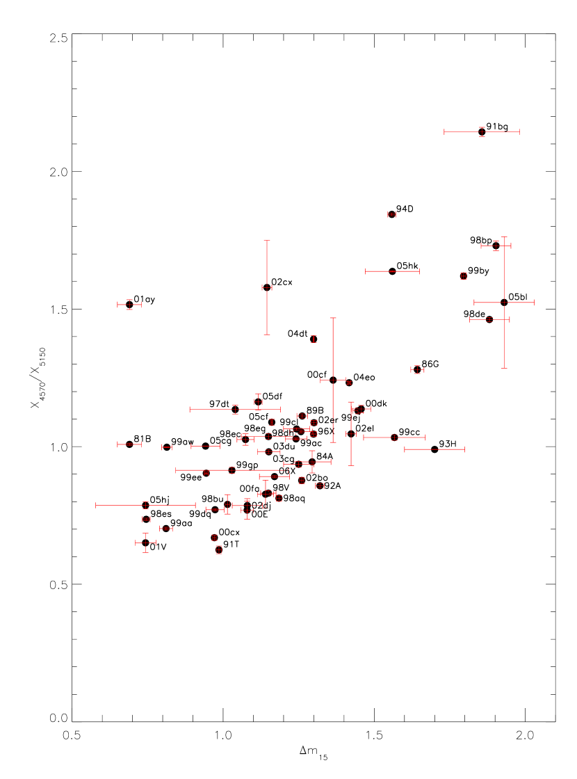
Due to the restriction on the 4570 Å feature, the same restriction to spectra within 5 days of maximum is applied to Figure 13. This ratio may be a useful parameter for the slower decliners but not for fast decliners.

4.7 Extinction

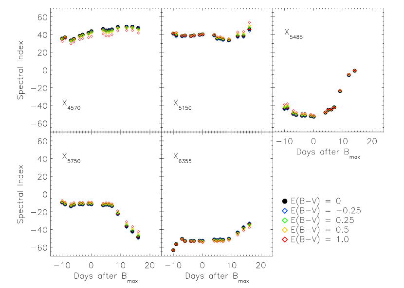
To explore the impact of reddening on the spectral indices, each spectra in the supernova sample in Table 4.1 was reddened. Four values for E(B-V) were chosen: -0.25, 0.25, 0.5, and 1.0. An identical procedure to that described in Section 3 was applied to these reddened spectra and spectral indexes were recalculated.

Figure 14: Same as Figure 7, but with the spectral indices recomputed separately for each of the 4 E(B-V) values.

Figure 15: Same as Figure 8, but with the addition of four panels each displaying the spectral indices for four values of E(B-V). The lower right panel overlays data from the first five panels.

Figures 14 and 15 are similar to Figures 7 and 8, but now include the effects of various values of E(B-V). Figures 14 and 15 together demonstrate that reddening has only a minor effect on spectral indices and is, in any event, an effect that can be corrected.

5 Conclusions

Efforts to correlate the intrinsic brightness of Type Ia supernovae with spectral line ratios or other methods related to feature strength are considerably complicated by line blending and noise. We introduce a comparatively new technique to astronomical image processing based on an à trous wavelet decomposition and use it to extract spectral strengths of Type Ia supernovae. In a straightforward manner repeated application of the à trous generates successively smoother scales. The lowest scale can be identified with noise; a smooth residual results from truncating the algorithm at the highest scale. The intermediate scales are those that can be identified with spectral features and combining several of these intermediate scales provides a robust measure of spectral strength without having to wrestle with integration limits or a definition of the continuum. Monte Carlo methods in conjunction with a very high SNR Type Ia supernova spectrum allows for correction of the spectral indices of supernovae with lower SNR, even those whose SNR approach one. These same methods readily permit error bars to be assigned to the spectral indices. The result is a definition of spectral line strength that is applied in this paper to the temporal evolution of spectral line strengths and the correlation of important spectral features with $\Delta m_{15}$. These indices are also shown to be largely impervious to reddening. A more robust spectral line strength like that developed here is likely to advance the identification or study of Type Ia subtypes or permit the construction of Type Ia templates with stretches that differ from unity. The latter effort, in particular, is directly related to our work on photometric redshift estimation for the next generation of ground- and spaced-based survey telescopes.

References

- Altavilla et al. (2007) Altavilla, G., et al. 2007, A&A, 475, 585
- Altavilla et al. (2009) Altavilla, G., et al. 2009, ApJ, 695, 135
- Anupama (1997) Anupama, G. C. 1997, AJ, 114, 2054
- Anupama et al. (2005) Anupama, G. C., Sahu, D. K., & Jose, J. 2005, A&A, 429, 667
- Arsenijevic et al. (2008) Arsenijevic, V., Fabbro, S., Mourão, A. M., & Rica da Silva, A. J. 2008, A&A, 492, 535
- Bailey et al. (2009) Bailey, S., et al. 2009, arXiv:0905.0340
- Barbon et al. (1989) Barbon, R., Rosino, L., & Iijima, T. 1989, A&A, 220, 83
- Barbon et al. (1990) Barbon, R., Benetti, S., Rosino, L., Cappellaro, E., & Turatto, M. 1990, A&A, 237, 79
- Benetti et al. (2004) Benetti, S., et al. 2004, MNRAS, 348, 261
- Benetti et al. (2005) Benetti, S., et al. 2005, ApJ, 623, 1011
- Bongard et al. (2006) Bongard, S., Baron, E., Smadja, G., Branch, D., & Hauschildt, P. H. 2006, ApJ, 647, 513
- Bongard et al. (2008) Bongard, S., Baron, E., Smadja, G., Branch, D., & Hauschildt, P. H. 2008, ApJ, 687, 456
- Branch et al. (1983) Branch, D., Lacy, C. H., McCall, M. L., Sutherland, P. G., Uomoto, A., Wheeler, J. C., & Wills, B. J. 1983, ApJ, 270, 123
- Branch et al. (2003) Branch, D., et al. 2003, AJ, 126, 1489
- Branch et al. (2004) Branch, D., Baron, E., Thomas, R. C., Kasen, D., Li, W., & Filippenko, A. V. 2004, PASP, 116, 903
- Branch et al. (2006) Branch, D., et al. 2006, PASP, 118, 560
- Branch et al. (2009) Branch, D., Dang, L. C., & Baron, E. 2009, PASP, 121, 238
- Elias-Rosa et al. (2006) Elias-Rosa, N., et al. 2006, MNRAS, 369, 1880
- Filippenko et al. (1992a) Filippenko, A. V., et al. 1992a, ApJ, 384, L15
- Filippenko et al. (1992b) Filippenko, A. V., et al. 1992b, AJ, 104, 1543
- Folatelli (2003) Folatelli, G., 2003, Spectral homogeneity of type Ia supernovae
- Garavini et al. (2004) Garavini, G., et al. 2004, AJ, 128, 387
- Garavini et al. (2005) Garavini, G., et al. 2005, AJ, 130, 2278
- Garavini et al. (2007) Garavini, G., et al. 2007, A&A, 470, 411
- Garavini et al. (2007) Garavini, G., et al. 2007, A&A, 471, 527
- Garnavich et al. (2004) Garnavich, P. M., et al. 2004, ApJ, 613, 1120
- Hachinger et al. (2006) Hachinger, S., Mazzali, P. A., & Benetti, S. 2006, MNRAS, 370, 299
- Hamuy et al. (2002) Hamuy, M., et al. 2002, AJ, 124, 417
- Harris et al. (1983) Harris, G. L. H., Hesser, J. E., Massey, P., Peterson, C. J., & Yamanaka, J. M. 1983, PASP, 95, 607
- Hernandez et al. (2000) Hernandez, M., et al. 2000, MNRAS, 319, 223
- Hicken et al. (2007) Hicken, M., Garnavich, P. M., Prieto, J. L., Blondin, S., DePoy, D. L., Kirshner, R. P., & Parrent, J. 2007, ApJ, 669, L17
- Holtschneider et al. (1989) Holtschneider, M, Kronland-Martinet, R., Morlet, J., Tchamitchian. P., In: Wavelets, Time-Frequency Methods and Phase Space, Springer-Verlag, Berlin, 289–297, 1989
- Howell & Nugent (2004) Howell, A., & Nugent, P. 2004, Cosmic explosions in three dimensions, 151
- Howell et al. (2006) Howell, D. A., et al. 2006, Nature, 443, 308
- Jha et al. (1999) Jha, S., et al. 1999, ApJS, 125, 73
- Jha et al. (2006) Jha, S., Branch, D., Chornock, R., Foley, R. J., Li, W., Swift, B. J., Casebeer, D., & Filippenko, A. V. 2006, AJ, 132, 189
- Kirshner et al. (1993) Kirshner, R. P., et al. 1993, ApJ, 415, 589
- Kotak et al. (2005) Kotak, R., et al. 2005, A&A, 436, 1021
- Krisciunas et al. (2007) Krisciunas, K., et al. 2007, AJ, 133, 58
- Leibundgut et al. (1991) Leibundgut, B., Kirshner, R. P., Filippenko, A. V., Shields, J. C., Foltz, C. B., Phillips, M. M., & Sonneborn, G. 1991, ApJ, 371, L23
- Leibundgut et al. (1993) Leibundgut, B., et al. 1993, AJ, 105, 301
- Li et al. (1999) Li, W. D., et al. 1999, AJ, 117, 2709
- Li et al. (2001) Li, W., et al. 2001, PASP, 113, 1178
- Li et al. (2003) Li, W., et al. 2003, PASP, 115, 453
- Matheson et al. (2008) Matheson, T., et al. 2008, AJ, 135, 1598
- Mazzali et al. (1993) Mazzali, P. A., Lucy, L. B., Danziger, I. J., Gouiffes, C., Cappellaro, E., & Turatto, M. 1993, A&A, 269, 423
- Mazzali et al. (2008) Mazzali, P. A., Sauer, D. N., Pastorello, A., Benetti, S., & Hillebrandt, W. 2008, MNRAS, 386, 1897
- Meikle et al. (1996) Meikle, W. P. S., et al. 1996, MNRAS, 281, 263
- Meikle & Hernandez (2000) Meikle, P., & Hernandez, M. 2000, Memorie della Societa Astronomica Italiana, 71, 299
- Nugent et al. (1995) Nugent, P., Phillips, M., Baron, E., Branch, D., & Hauschildt, P. 1995, ApJ, 455, L147
- Patat et al. (1996) Patat, F., Benetti, S., Cappellaro, E., Danziger, I. J., della Valle, M., Mazzali, P. A., & Turatto, M. 1996, MNRAS, 278, 111
- Perlmutter et al. (1997) Perlmutter, S., et al. 1997, ApJ, 483, 565
- Riess et al. (1998) Riess, A. G., Nugent, P., Filippenko, A. V., Kirshner, R. P., & Perlmutter, S. 1998, ApJ, 504, 935
- Phillips et al. (1987) Phillips, M. M., et al. 1987, PASP, 99, 592
- Phillips et al. (1992) Phillips, M. M., Wells, L. A., Suntzeff, N. B., Hamuy, M., Leibundgut, B., Kirshner, R. P., & Foltz, C. B. 1992, AJ, 103, 1632
- Phillips et al. (2007) Phillips, M. M., et al. 2007, PASP, 119, 360
- Pignata et al. (2008) Pignata, G., et al. 2008, MNRAS, 388, 971
- Quimby et al. (2006) Quimby, R., Höflich, P., Kannappan, S. J., Rykoff, E., Rujopakarn, W., Akerlof, C. W., Gerardy, C. L., & Wheeler, J. C. 2006, ApJ, 636, 400
- Quimby et al. (2007) Quimby, R., Höflich, P., & Wheeler, J. C. 2007, ApJ, 666, 1083
- Ruiz-Lapuente et al. (1992) Ruiz-Lapuente, P., Cappellaro, E., Turatto, M., Gouiffes, C., Danziger, I. J., della Valle, M., & Lucy, L. B. 1992, ApJ, 387, L33
- Sahu et al. (2008) Sahu, D. K., et al. 2008, ApJ, 680, 580
- Salvo et al. (2001) Salvo, M. E., Cappellaro, E., Mazzali, P. A., Benetti, S., Danziger, I. J., Patat, F., & Turatto, M. 2001, MNRAS, 321, 254
- Starck et al. (1995) Starck, J.-L., Murtagh, F., & Bijaoui, A. 1995, Astronomical Data Analysis Software and Systems IV, 77, 279
- Starck et al. (1997) Starck, J.-L., Siebenmorgen, R., & Gredel, R. 1997, ApJ, 482, 1011
- Stanishev et al. (2007) Stanishev, V., et al. 2007, A&A, 469, 645
- Strolger et al. (2002) Strolger, L.-G., et al. 2002, AJ, 124, 2905
- Taubenberger et al. (2008) Taubenberger, S., et al. 2008, MNRAS, 385, 75
- Turatto et al. (1996) Turatto, M., Benetti, S., Cappellaro, E., Danziger, I. J., Della Valle, M., Gouiffes, C., Mazzali, P. A., & Patat, F. 1996, MNRAS, 283, 1
- Valentini et al. (2003) Valentini, G., et al. 2003, ApJ, 595, 779
- Wang et al. (1997) Wang, L., Wheeler, J. C., & Hoeflich, P. 1997, ApJ, 476, L27
- Wang et al. (2003) Wang, L., et al. 2003, ApJ, 591, 1110
- Wang et al. (2006) Wang, L., Strovink, M., Conley, A., Goldhaber, G., Kowalski, M., Perlmutter, S., & Siegrist, J. 2006, ApJ, 641, 50
- Wang et al. (2008) Wang, X., et al. 2008, ApJ, 675, 626
- Wells et al. (1994) Wells, L. A., et al. 1994, AJ, 108, 2233