The absorption-dominated model for the X-ray spectra of type I active galaxies: MCG–6-30-15

Abstract

MCG–6-30-15 is the archetypal example of a type I active galaxy showing broad “red-wing” emission in its X-ray spectrum at energies below the 6.4 keV Fe K$\alpha$ emission line and a continuum excess above 20 keV. Miller et al. (2008) showed that these spectral features could be caused by clumpy absorbing material, but Reynolds et al. (2009) have argued that the observed Fe K$\alpha$ line luminosity is inconsistent with this explanation unless the global covering factor of the absorber(s) is very low. However, the Reynolds et al. calculation effectively considers the only source of opacity to be the Fe K bound-free transition and neglects the opacity at the line energy: correction to realistic opacity decreases the predicted line flux by a large factor. We also discuss the interpretation of the covering factor and the possible effect of occultation by the accretion disk. Finally, we consider a model for MCG–6-30-15 dominated by clumpy absorption, which is consistent with global covering factor 0.45, although models that include the effects of Compton scattering are required to reach a full understanding. Variations in covering fraction may dominate the observed X-ray spectral variability.

1 Introduction

MCG–6-30-15 is a $z=0.00775$ type I active galaxy that was one of the first discovered to have in its X-ray spectrum a broad “red wing” of emission below the 6.4 keV Fe K$\alpha$ line (Tanaka et al., 1995). This has been interpreted as reflected emission from an accretion disk, occurring so close to the black hole that relativistic effects redshift the Fe K$\alpha$ line over a wide observed energy range (e.g. Iwasawa et al., 1996; Wilms et al., 2001; Fabian & Vaughan, 2003), an effect often known as “blurring”. Its significance is that it may allow us to observe accretion close to the black hole and even infer the black hole angular momentum, if highly-redshifted emission is measured (e.g. Brenneman & Reynolds, 2006).

However, the X-ray spectra may also be interpreted as being dominated by the effects of absorption by material further away from the black hole, albeit still at interesting radii (e.g. Inoue & Matsumoto, 2003). Recently, Miller, Turner & Reeves (2008, hereafter MTR) have shown that the substantial X-ray dataset for MCG–6-30-15, comprising Chandra HETG, XMM-Newton EPIC-pn and RGS and Suzaku XIS and HXD-PIN observations, between them covering the range 0.5–40 keV, could be fitted by an absorption-dominated model with no relativistically-blurred emission. MTR’s analysis remains the only one to date to systematically analyse this multi-observatory dataset across the whole available spectral range and modelling the observed range of spectral variability. The model described well that spectral variability, from a low, more absorbed-looking state to a higher, less absorbed state, as well as the absorption lines observed in the grating data. Such states are common in type I AGN (e.g. Miller et al., 2007). A key ingredient was that at least one of the absorbing zones should be “partial-covering”, implying the absorber is clumpy. Some of those zones are outflowing (Lee et al., 2001; Young et al., 2005) and MTR suggested the absorption is part of an accretion disk wind, enabling us to study the complex outflowing winds that are expected from AGN with high Eddington ratios (King & Pounds, 2003). The most absorbing zone in the MTR model is responsible for creating the excess seen in the Suzaku data above 20 keV.

As the absorbing gas is expected to be photoionised, we should see recombination and fluorescent emission, and in principle we can use its luminosity to constrain the global covering factor (i.e. the fraction of the sky covered by the absorber as seen from the ionising source) - see Turner & Miller (2009) for a review. A low line luminosity might imply that the covering factor is low and that our view through an absorber is an unusual sightline. Reynolds et al. (2009, hereafter R09) have tried to estimate the expected Fe K$\alpha$ fluorescent line luminosity expected from an absorption model for MCG–6-30-15 and have argued that the implied global covering factor is in the range 0.0175–0.035. They infer that we are unlikely to be on a sightline through the absorber, and argue that this model is disfavoured compared with the relativistically-blurred interpretation of the X-ray spectra.

In this letter we show that the calculation of R09 makes poor assumptions that invalidate their conclusion and we discuss additional effects that may change the interpretation of such analysis. Also, R09 chose not to test the actual model described by MTR, so here we discuss constraints on the global covering factor in that model. MTR supposed the hard excess to arise from a combination of absorption and reflection, but the composition of this component is not well constrained by the data. A number of AGN have recently been discovered to have hard X-ray excesses that appear best explained by clumpy absorption alone (e.g. Turner et al., 2009), so here we also test a model, suggested by MTR but not tested at that time, in which the spectrum and its variability are shaped by such high-opacity, clumpy absorption.

2 Fluorescent line emission from absorbing zones

To place limits on the absorber covering factor in MCG–6-30-15, R09 approximately fit the Suzaku data, finding that an absorbing zone of cold gas with column density $2\times 10^{24}$ cm^-2 and covering fraction $C_{f}\simeq 0.35$ can reproduce the observed hard X-ray excess. We define $C_{f}$ to be the fraction of the source covered by the absorber as seen by the observer, and the global covering factor $C_{g}$ to be the fraction of the sky covered by the absorber as seen from the source. R09 estimated that the zone absorbs $7.3\times 10^{-4}$ photons s^-1 cm^-2 from the incident spectrum seen by an observer in the rest-frame energy range $7.08-20$ keV. They assumed all these photons are absorbed by the Fe K bound-free transition, with Fe K fluorescent yield 0.347, leading to an expected Fe K (not K$\alpha$) line flux of $2.54\times 10^{-4}$ photons s^-1 cm^-2. The calculation is inadequate for two reasons.

• Near the Fe K absorption edge, that transition only accounts for a fraction 0.51 of the total photoelectric opacity in low ionisation material (Verner et al., 1996), causing R09 to have overestimated the line flux by a factor about 2.

• Line photons produced within the absorber are absorbed as they pass through it. The R09 absorber has optical depth at Fe K$\alpha$ $\tau\simeq 3.5$, given by the phabs function in xspec (Arnaud, 1996), so reabsorption of line photons cannot be neglected.

In effect, the R09 calculation assumes that the only source of opacity is the Fe K bound-free transition, ignoring the opacity from other ions and from the outer shells of Fe. To find the effect of these omissions we calculated the expected line emission from a spherical cloud, of constant density, absorbing photons from a distant ionising source. The gas was assumed to be cold, as in R09, with solar abundances (Anders & Grevesse, 1989) and cross-sections of Verner et al. (1996). For comparison with R09, we first calculate the line emission by integrating over the volume of the sphere, taking account of the inward and outward optical depths as a function of viewing angle, omitting the effects of Compton scattering. Fig. 1 shows the results for a sphere with mean column density $2\times 10^{24}$ cm^-2, illuminated by a power-law of photon index $\Gamma=2.2$ and normalisation that would be seen by the observer in the absence of absorption of 1 photon s^-1cm^-2keV^-1 at 1 keV. As the cloud does not surround the ionising source, the line flux in Fig. 1 should be multiplied by the global covering factor of the cloud. Also shown is the expected value as calculated by R09: i.e. measuring the flux removed in the energy range $7.08-20$ keV and multiplying by a fluorescent yield of 0.347. For a view through the absorber, the line flux is a factor 11 lower than predicted by R09. Even viewing the front illuminated face, when line photons have the highest escape probability, the line flux is a factor 3.7 lower than predicted by R09. The factor by which the R09 calculation overpredicts the line flux depends only weakly on $\Gamma$.

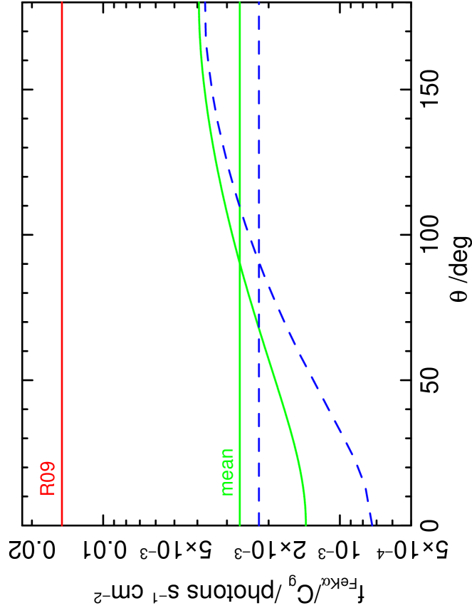
Figure 1: The Fe K$\alpha$ line flux expected from the spherical cloud, as a function of viewing angle, $\theta$, defined to be zero looking through the absorber towards the ionising source, not including the effects of Compton scattering (solid curve). Also shown is the mean line flux averaged over viewing angles assuming an isotropic distribution of clouds (lower solid horizontal line) and the result from the calculation of R09 (upper line). The dashed curve shows the results for the calculation including Compton scattering.

Suppression of the line flux by photoelectric absorption is inevitable: if there is sufficient column density to produce detectable line emission there must also be sufficient opacity to absorb line photons. However, the assumed geometry of a system of clouds affects the predictions. If they isotropically surround the source, we can calculate an upper limit to the total line flux expected from the ensemble, averaging over viewing angles, if we neglect “clouds covering clouds”. This flux is also shown on Fig. 1 and is a factor 5.7 lower than the R09 prediction. If the cloud-on-cloud covering factor of the source were 0.35, the line emission would be reduced by about this factor. The absorbing system likely has a more complex geometry, but, for any distribution, significantly less line emission is expected than predicted by R09.

However, such a high column-density absorber has an optical depth to Compton scattering $\tau_{C}\simeq 1.6$, so Fig. 1 also shows the line emission predicted by a Monte Carlo calculation that includes Compton scattering (see also Nandra & George 1994 and Murphy & Yaqoob 2009). For comparison, the front-illuminated equivalent width against the illuminating continuum is 220 eV, close to the value, scaled to full covering, of 280 eV for reflection from an optically-thick disk (George & Fabian, 1991). For a given illuminating continuum, the line emission is lower than the case without Compton scattering. Fitting models to data becomes more dependent on absorber geometry, however, because the transmitted continuum flux is attenuated by Compton scattering, but Compton-scattered light from other clouds enters our line of sight to compensate: there is scattered continuum whose amplitude is closely linked to the scattered line flux. A full calculation of the expected line flux should take into account the effects of Compton scattering from the ensemble of clouds, with some assumed geometry.

3 The covering factor

Before proceeding, we should consider what is meant by the global covering factor, $C_{g}$, in the case where the absorber has a complex structure. Suppose a wind from the accretion disk subtends solid angle $\Omega$ at the ionising source, but that within the wind, absorbing material is fragmented into many clumps that are much smaller than the projected size of the emitting source: the absorbing clumps might themselves cover a fraction $f$ of the wind. In this case the expected line luminosity $L_{\rm line}\propto\Omega f$. But the probability that a randomly-oriented observer would lie on a sightline passing through the wind is $p\simeq\Omega/4\pi$, without the $f$ factor, and all such sightlines would see the source covered by the fraction $C_{f}=f$. In the R09 model, $C_{f}=0.35$ and R09 would infer $C_{g}=\Omega f/4\pi\simeq 0.035$, but in this case the wind covering factor would be $C_{g}=\Omega/4\pi\simeq 0.1$, significantly higher than the covering factor inferred for the individual clumps within the wind. Realistic, complex winds are unlikely to be described by just two numbers, further adding to the inherent uncertainty in sightline probability.

In the case where the absorbers are part of a disk wind, we could reasonably expect the accretion disk to extend over at least the same radii as the wind material. In this case an observer only sees half of the line-emitting material, the other half being obscured by the accretion disk (Turner et al., 2009). If we make the standard assumption that the material is exposed to the same ionising intensity that the observer infers, this occultation introduces up to a further factor 2 into the estimate of the wind covering factor irrespective of whether or not the source itself is occulted.

4 The MTR model

The consequence of such large factors missing from the R09 estimate is that the covering factor deduced could rise from 0.035 to $\ga 0.5$. However, R09 did not carry out any calculations for the actual model fitted to the MCG–6-30-15 data by MTR. This has ionised absorbing zones, which might be expected to increase the line flux for a given high-energy excess, as the relative importance of Fe K absorption is expected to increase and the fluorescent yield around Fe XIX is higher than for lower ions (e.g. Kallman et al., 2004). On the other hand, the column densities required were significantly lower than assumed by R09. We start by considering the line emission expected from the MTR model.

There were two key zones, one with $N_{H}\simeq 4\times 10^{22}$ cm^-2 partially-covering the primary X-ray source, designated “zone 5”, and a second with $N_{H}\simeq 5\times 10^{23}$ cm^-2 covering only a component of reflected emission, designated “zone 4”. Note that MTR’s first three absorbing zones, labelled 1–3, are low opacity columns previously discussed by Lee et al. (2001), Turner et al. (2003, 2004) and Young et al. (2005). These produce insignificant line emission. Although the “3+2” zone model requires the introduction of appropriate free parameters in the fit, zones 1–3 are clearly required by the presence of narrow absorption lines in the XMM-Newton and Chandra grating data and cannot be ignored, particularly if we wish to model the entire source spectrum, not a selected sub-region. The total number of free parameters required is fewer than in other analyses (e.g. Brenneman & Reynolds, 2006) and yet the models provide a good description of the entire 0.5-50 keV spectrum across multiple datasets, tested against the full observed range of spectral states. There is substantial additional information in the spectral variability that is missed by fitting only to the mean spectrum.

Consider first zone 5. This low column is primarily responsible for the spectral curvature in the “red wing” at 2–6 keV (see Fig. 4 of MTR). Absorption models were generated using xstar (Kallman & Bautista, 2001; Kallman et al., 2004) 2.1ln11 and we estimated the expected line strength from the xstar emission-line table. The xstar line luminosities are those expected from a source with 1–1000 Ry luminosity $10^{38}$ erg s^-1 at a distance of 1 kpc: these values were scaled to the amplitude of a power-law continuum integrated over that energy range, yielding a normalisation factor 0.01695 for a power-law with photon index $\Gamma=2.2$ and amplitude 1 photon s^-1 cm^-2 keV^-1 at 1 keV. As the optical depth at Fe K$\alpha$ is only 0.05 in this zone, the result is independent of viewing angle. For $C_{g}=0.35$, we find a predicted Fe K$\alpha$ line flux of $2.9\times 10^{-6}$ photons s^-1 cm^-2, which does not provide any constraint on the global covering factor of this zone, as the predicted flux is a factor 8 below the observed line flux of $2.5\times 10^{-5}$ photons s^-1 cm^-2 (R09).

Zone 4 of MTR had column density of $5.49\times 10^{23}$ cm^-2 and ionisation parameter $\log\xi=1.94$, covering reflected emission modelled by reflionx (Ross & Fabian, 2005). reflionx includes line emission, but calculating the line luminosity from the absorbing zone is more problematic, as the geometry is unknown, and the reflector line emission itself is a function of orientation, not modelled in reflionx. As the optical depth of zone 4 at Fe K$\alpha$ is $\tau\simeq 0.4$, its line flux also has some weak orientation dependence. Thus the following estimate can only be approximate. Since the Fe K$\alpha$ flux is determined by photons absorbed above the K-edge, we use the total high energy continuum flux to estimate the expected line strength. The total source flux at 20 keV was $f(E)\simeq 0.0015$ keV s^-1cm^-2keV^-1: extrapolating over 1–1000 Ry assuming $\Gamma=2.2$ and using the zone 4 xstar table we find an expected Fe K$\alpha$ line flux of $5\times 10^{-6}$ photons s^-1cm^-2 assuming full covering. This is a factor 5 below the observed flux and does not strongly constrain the MTR model.

While full covering of optically-thick material is not physical, a high covering is needed to obtain sufficient reflected flux: MTR reported that the nominal reflection factor with respect to reflection from a disk subtending 2$\pi$ sr is $R\simeq 1.7$, and they suggested that, instead, further highly absorbed zones are likely responsible for a greater proportion of the hard excess than in the baseline model. A further problem for the baseline MTR model is that the ionised absorber zone 4 may also produce soft-band O vi - viii line emission, which is not observed in the grating data, implying either that the Fe/O abundance ratio is enhanced or that the highest column density zones should have lower ionisation than fitted by MTR.

5 A pure absorption model

In the MTR model, absorbed reflection dominates the hard excess, but the composition of this component is not well constrained by the data. More recently, evidence has been found for hard excesses caused by high-column partial-covering absorption, in 1H 0419-577 (Turner et al., 2009), PDS 456 (Reeves et al., 2009) and NGC 1365 (Risaliti et al., in preparation), so we now investigate an extreme model, discussed by MTR, where all of the hard excess is produced by absorbing, rather than reflecting, zones. R09 argue that the line emission from such a model should be representative of the whole class of models explaining the hard excess, for the purposes of estimating the covering factor.

Table 1: Absorber model parameters, giving for each zone the column density, ionisation parameter and mean covering fraction, $\overline{C_{f}}$. $C_{f}$ was variable for zones 4 & 5. Confidence intervals are 68%. Quantities in brackets were fixed in the Suzaku analysis.

zone	N /$10^{22}$cm-2	log($\xi$/erg cm s-1)	$\overline{C_{f}}$
1	1.18$\pm.05$	$2.39\pm.01$	(1.0)
2	0.027$\pm.003$	$0.88\pm.16$	(1.0)
3	(8.0)	(3.95)	(1.0)
4	191.$\pm 30$	-	0.62
5	2.9$\pm.1$	$1.38\pm.03$	0.17

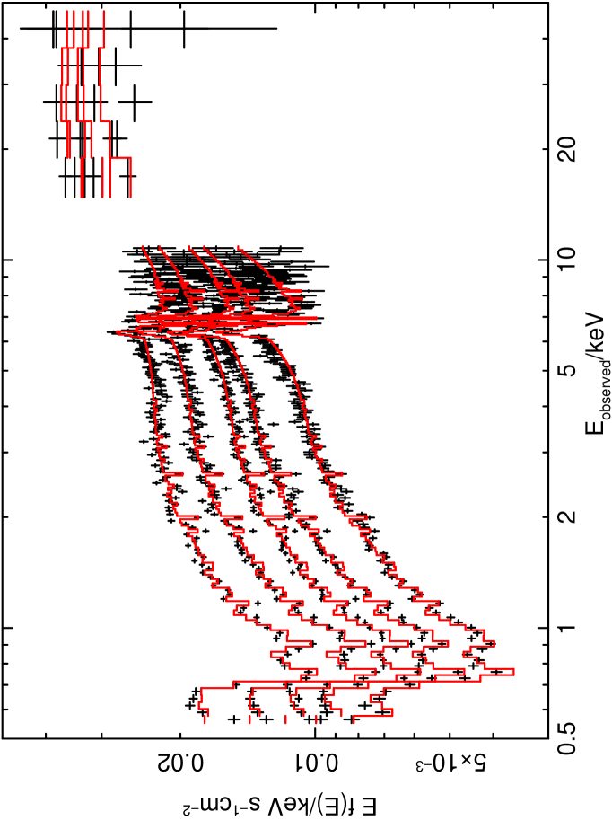
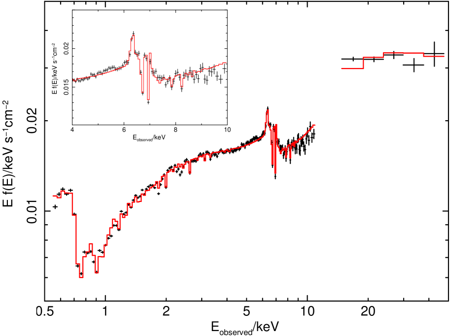
Figure 2: Model fit to the Suzaku data: (left) divided into five flux states; (right) the mean spectrum, with insert zoom-in showing the 4–10 keV region with linear axes. The model is shown in units of Ef(E), points with error bars show the “unfolded” data.

To test models of MCG–6-30-15, we use the datasets reduced and analysed by MTR, adopting the same division into flux states. We emphasise the importance, when $\chi^{2}$-fitting, of using data binned to match the energy-dependent instrument resolution: finer bins result in significantly less sensitivity to departures from the model (section 2.1 of MTR). Coarser bins are allowed, provided that does not erase spectral features. It is also important to account for systematic errors (section 2.2 of MTR) and we likewise adopt here a systematic fractional error of 0.03, a likely lower limit to the calibration uncertainty given cross-instrument comparisons that show energy-dependent differences of 5–20% (Stuhlinger, 2007). This has a significant effect when fitting over the full energy range, as otherwise the goodness-of-fit is determined almost entirely, but erroneously, by the soft band where shot noise uncertainty is very small, reducing the accuracy of the model in the crucial Fe K region. Previous analyses have relied on using data binning that is too fine, and often not including the soft band in the analysis, to obtain apparently good fits (e.g. Miniutti et al.2007; R09).

To construct the model, we replaced MTR’s absorbed reflection (zone 4 absorbing reflionx) by a single zone of absorption partially-covering the continuum. This component has a very hard spectrum and likely comprises a high column density of low ionisation gas. We cannot now predict the line luminosity using xstar as the zone is optically-thick at Fe K$\alpha$, and we must take account of the angular dependence of the line emission. However, a good fit to the data may be obtained by assuming this zone to be cold gas with transmitted flux modelled by the uniform-density sphere of section 2, so we use those results to estimate $C_{g}$. In this simple model we ignore Compton scattering, so the transmitted flux fraction is $f(E)=2\int_{0}^{1}\exp\left[-\frac{3}{2}N\sigma_{E}\left(1-z^{2}\right)^{1/2}\right]z\mathrm{d}z$ where $N$ is the mean column density and $\sigma_{E}$ is the energy-dependent absorption cross-section. Fe K$\alpha$, K$\beta$ line emission was added to the model with line ratio 0.135 (Leahy & Creighton, 1993). We convolved the line emission with a gaussian FWHM 4000 km s^-1, consistent with the line width in the Chandra data.

As we now use xstar 2.1ln11 the parameters of zone 3 were redetermined from the Chandra HEG data, and we found a velocity dispersion of 1000 km s^-1 best matched the data. We include xstar line emission from zone 5 in the fit, although its global covering factor is not constrained, so we fix $C_{g}=0.2$ (including the factors in section 3). Fitting simultaneously to the Suzaku multiple flux states over the energy range $0.55-50$ keV, we found a goodness-of-fit of $\chi^{2}=728$ for 844 degrees of freedom (dof). Absorber parameters are given in Table 1, best-fit photon index was $\Gamma=2.20\pm 0.003$ and Galactic column density $4.2\pm 0.3\times 10^{20}$cm^-2. The 0.7 keV edge depth was degenerate with the zone 2 parameters and so was fixed at $\tau=0.45$. Fitting to the mean spectrum, with all parameters other than normalisations fixed to the multiple flux-state values, resulted in $\chi^{2}=119$ for 170 dof. There is some indication of a slight model excess in the region of the Fe K edge (Fig. 2) but Compton scattering in the high column-density absorber and some degree of ionisation are both expected to soften the edge. Strictly, zone 2 is not required by the Suzaku data, but is required by the absorption lines in the Chandra data (Lee et al., 2001). Fitting the same model to the Chandra data allowing only component normalisations to change resulted in $\chi^{2}=3538$ for 3346 dof. Allowing the warm absorber parameters to vary resulted in $\chi^{2}=3427$ for 3341 dof, showing good agreement with the high resolution mean spectrum. This model is not unique, and does not include any scattered continuum (see below), but the goodness-of-fit is already sufficiently good that, statistically, no additional components are justified.

The Fe K$\alpha$ flux (assumed constant) was $2.27\pm 0.2\times 10^{-5}$ photon s^-1 cm^-2, the mean continuum flux incident on the absorber was $0.0383\pm 0.0012$ photons s^-1cm^-2keV^-1 at 1 keV. Using the section 2 line flux for $N_{H}=1.9\times 10^{24}$ cm^-2, we infer a mean global covering factor $C_{g}\simeq 0.45\pm.04$ (statistical errors only, 68% confidence intervals), including the factors in section 3.

However, as noted in section 2, the optical depth to Compton scattering in this absorber would be $\tau_{C}\simeq 1.5$, so the true incident flux onto this component could be a factor 5 higher than inferred and the deduced mean covering fraction, $\overline{C_{f}}$, could be substantially closer to unity after allowance for scattering. The hard-band flux would also have a significant contribution from light scattered into our line of sight from the other absorbers around the source (the “absorbed reflected” component in the original MTR model may be a representation of such a Compton-scattered component). To achieve a better measure of $C_{g}$ we need to model the spectrum that is scattered into our line of sight (Miller et al., in preparation).

6 Discussion

Much of the motivation for the work of MTR was the observation that the red wing and hard excess appear fairly constant, despite large variations in source brightness at $E<10$ keV. If these components are reflected emission then their brightness should vary in phase with the illuminating continuum, as the light travel time between source and inner accretion disk should be negligible. A popular explanation for the lack of such variation is the “light-bending” model of Fabian & Vaughan (2003), Miniutti et al. (2003) and Miniutti & Fabian (2004). Miniutti et al. (2003) show for MCG–6-30-15 that if the illuminating source is within about $3-4$ GM/c² of the black hole, and if it varies in height over about $3-8$ GM/c², then the effects of light following geodesics in the spacetime near the black hole mean that the flux reaching the distant observer from the source can be arranged to decrease as it approaches the accretion disk, while the observed flux reflected from the disk may remain approximately constant. In this picture the source variability is caused by motion of the central source: obtaining a relatively constant reflected intensity requires both the supposition of a compact vertically-moving source and its careful placement.

The alternative explanation presented here implies that a substantial fraction of the observed variability is caused by variations in covering fraction of clumpy absorbers. We suggest that the absorbers may be a complex multi-component structure, with a wide range of scale-sizes, possibly part of an accretion disk wind (e.g. Proga & Kallman, 2004). In this picture we expect the source variability to decrease to higher energy, as found for MCG–6-30-15, and that more absorbed AGN should show greater hard X-ray variability than less absorbed AGN, as found by Beckmann et al. (2007). There is expected to be reflection from the most optically-thick absorbers, but if the intrinsic source variations are low, both the reflection and any line emission would likewise be of relatively constant amplitude. The simple parameterisations presented here are likely not sufficient for detailed investigation of the X-ray spectra, and models of radiative transfer that treat scattering and absorption in the velocity field of the wind are needed (Sim et al., 2008).

7 Conclusions

The variability, “red wing” and hard excess in the X-ray spectrum of MCG–6-30-15 may all be explained by a model of clumpy absorption. The observed Fe K$\alpha$ line emission may be fluorescent emission from the absorbing material, in which case the global covering factor of the material is $C_{g}\simeq 0.45$. The largest uncertainty in this estimate is caused by lack of knowledge of the absorber geometry. In calculating the expected line emission it is essential to take account of photoelectric absorption of line photons, neglect of which could result in predictions that are incorrect by factors of order 10. Radiative transfer models that include the effect of Compton scattering are required to reach a full understanding of such systems. If correct, this model implies that a large fraction of the observed X-ray variability may be caused by variation in absorber covering fraction, and that a large fraction of the source $2-10$ keV luminosity may be partially obscured even in type I AGN.

Acknowledgments. We are grateful to Tim Kallman for providing and updating xstar. Rapid production of xstar tables was possible using pvm_xstar (Noble et al., 2009). TJT acknowledges NASA grant NNX08AJ41G.

References

- Anders & Grevesse (1989) Anders E., Grevesse N., 1989, Geochim. Cosmochim. Acta, 53, 197
- Arnaud (1996) Arnaud K. A., 1996, in Jacoby G. H., Barnes J., eds, ASP Conf. Ser. Vol. 101, Analysis Software and Systems V. Astron. Soc. Pac., San Francisco, p. 17
- Beckmann et al. (2007) Beckmann V., Barthelmy S. D., Courvoisier T. J.-L., Gehrels N., Soldi S., Tueller J., Wendt G., 2007, A&A, 475, 827
- Brenneman & Reynolds (2006) Brenneman L. W., Reynolds C. S., 2006, ApJ, 652, 1028
- Fabian & Vaughan (2003) Fabian A. C., Vaughan S., 2003, MNRAS, 340, L28
- George & Fabian (1991) George I. M., Fabian A. C., 1991, MNRAS, 249, 352
- Inoue & Matsumoto (2003) Inoue H., Matsumoto C., 2003, PASJ, 55, 625
- Iwasawa et al. (1996) Iwasawa K., Fabian A. C., Reynolds C. S. et al., 1996, MNRAS, 282, 1038
- Kallman & Bautista (2001) Kallman T., Bautista M., 2001, ApJS, 133, 221
- Kallman et al. (2004) Kallman T. R., Palmeri P., Bautista M. A., Mendoza C., Krolik J. H., 2004, ApJS, 155, 675
- King & Pounds (2003) King A. R., Pounds K. A., 2003, MNRAS, 345, 657
- Leahy & Creighton (1993) Leahy D. A., Creighton J., 1993, MNRAS, 263, 314
- Lee et al. (2001) Lee J. C., Ogle P. M., Canizares C. R., Marshall H. L., Schulz N. S., Morales R., Fabian A. C., Iwasawa K., 2001, ApJ, 554, L13
- Miller et al. (2008) Miller L., Turner T. J., Reeves J. N., 2008, A&A, 483, 437 (MTR)
- Miller et al. (2007) Miller L., Turner T. J., Reeves J. N., George I. M., Kraemer S. B., Wingert B., 2007, A&A, 463, 131
- Miniutti & Fabian (2004) Miniutti G., Fabian A. C., 2004, MNRAS, 349, 1435
- (17) Miniutti G., Fabian A. C., Anabuki N. et al., 2007, PASJ, 59, 315
- Miniutti et al. (2003) Miniutti G., Fabian A. C., Goyder R., Lasenby A. N., 2003, MNRAS, 344, L22
- Murphy & Yaqoob (2009) Murphy K. D., Yaqoob T., 2009, MNRAS, in press, arXiv:0905.3188
- Nandra & George (1994) Nandra K., George I. M., 1994, MNRAS, 267, 974
- Noble et al. (2009) Noble M. S., Ji L., Young A., Lee J., 2009, ArXiv:0901.1582
- Proga & Kallman (2004) Proga D., Kallman T. R., 2004, ApJ, 616, 688
- Reeves et al. (2009) Reeves, J. N., O’Brien, P. T., Braito, V. et al., 2009, ApJ, in press, arXiv:0906.0312
- Reynolds et al. (2009) Reynolds C. S., Fabian A. C., Brenneman L. W., Miniutti G., Uttley P., Gallo L. C., 2009, MNRAS, in press (R09)
- Ross & Fabian (2005) Ross R. R., Fabian A. C., 2005, MNRAS, 358, 211
- Sim et al. (2008) Sim S. A., Long K. S., Miller L., Turner T. J., 2008, MNRAS, 388, 611
- Stuhlinger (2007) Stuhlinger, M., 2007, Report to the XMM-Newton Users Group, 7-8 June 2007, http://xmm.vilspa.esa.es/ external/xmm_user_support/usersgroup/20070607/
- Tanaka et al. (1995) Tanaka Y., Nandra K., Fabian A. C. et al., 1995, Nature, 375, 659
- Turner et al. (2004) Turner A. K., Fabian A. C., Lee J. C., Vaughan S., 2004, MNRAS, 353, 319
- Turner et al. (2003) Turner A. K., Fabian A. C., Vaughan S., Lee J. C., 2003, MNRAS, 346, 833
- Turner & Miller (2009) Turner T. J., Miller L., 2009, A&A Rev., 17, 47
- Turner et al. (2009) Turner T. J., Miller L., Kraemer S. B., Reeves J. N., Pounds K. A., 2009, ApJ, 698, 99
- Verner et al. (1996) Verner D. A., Ferland G. J., Korista K. T., Yakovlev D. G., 1996, ApJ, 465, 487
- Wilms et al. (2001) Wilms J., Reynolds C. S., Begelman M. C., Reeves J., Molendi S., Staubert R., Kendziorra E., 2001, MNRAS, 328, L27
- Young et al. (2005) Young A. J., Lee J. C., Fabian A. C., Reynolds C. S., Gibson R. R., Canizares C. R., 2005, ApJ, 631, 733