Pseudogap, non-Fermi-liquid behavior, and particle-hole asymmetry
in the 2D Hubbard model

Abstract

The effect of doping in the two-dimensional Hubbard model is studied within finite temperature exact diagonalization combined with cluster dynamical mean field theory. By employing a mixed basis involving cluster sites and bath molecular orbitals for the projection of the lattice Green’s function onto $2\times 2$ clusters, a considerably more accurate description of the low frequency properties of the self-energy is achieved than in a pure site picture. The transition from Fermi-liquid to non-Fermi-liquid behavior for decreasing hole doping is studied as a function of Coulomb energy, next-nearest neighbor hopping, and temperature. In particular, the self-energy component $\Sigma_{X}$ associated with $X=(\pi,0)$ is shown to exhibit an onset of non-Fermi-liquid behavior as the hole doping decreases below a critical value $\delta_{c}$. The imaginary part of $\Sigma_{X}(\omega)$ then develops a collective mode above $E_{F}$, which exhibits a distinct dispersion with doping. Accordingly, the real part of $\Sigma_{X}(\omega)$ has a positive slope above $E_{F}$, giving rise to an increasing particle-hole asymmetry as the system approaches the Mott transition. This behavior is consistent with the removal of spectral weight from electron states close to $E_{F}$ and the opening of a pseudogap which increases with decreasing doping. The phase diagram reveals that $\delta_{c}\approx 0.15\ldots 0.20$ for various system parameters. For electron doping, the collective mode of $\Sigma_{X}(\omega)$ and the concomitant pseudogap are located below the Fermi energy which is consistent the removal of spectral weight from hole states just below $E_{F}$. The critical doping which marks the onset of non-Fermi-liquid behavior, is systematically smaller than for hole doping.
         
PACS. 71.20.Be Transition metals and alloys - 71.27+a Strongly correlated electron systems

I Introduction

The nature of the metal insulator transition as a function of doping is one of the key issues in strongly correlated materials. imada Experimental studies of many high-$T_{c}$ cuprates reveal a rich phase diagram, with conventional Fermi-liquid behavior in overdoped metals and an anomalous pseudogap phase in underdoped systems close to the Mott insulator. One of the most intriguing and challenging aspects of the non-Fermi-liquid phase is the observation of highly non-isotropic behavior in momentum space. norman Whereas along the nodal direction $\Gamma M$ well-defined quasiparticles exist, in the vicinity of $X=(\pi,0)$ strong deviations from Fermi-liquid behavior occur. In particular, below a critical doping a pseudogap appears which becomes more prominent close to the Mott insulator. This transition from Fermi-liquid to non-Fermi-liquid properties has been widely investigated in recent years, and several theoretical models have been proposed. pwa ; wen ; kivelson ; varma ; vojta ; Chakravarty ; honerkamp ; lauchli ; konik ; yang1 ; tsvelik ; sachdev ; phillips

Dynamical mean field theorydmft1 ; dmft2 ; dmft3 ; dmft4 ; dmft5 ; dmft (DMFT) provides an elegant and successful framework for the description of the correlation induced transition from metallic to Mott insulating behavior. reviews The local or single-site version of DMFT, however, focusses exclusively on dynamical correlations which can give rise to spectral weight transfer between low and high frequencies. To address the momentum dependence of the self-energy, it is important to allow for spatial fluctuations, at least on a short-range atomic scale. For this purpose, several approaches based on cluster extensions of DMFT hettler ; lichtenstein ; kotliar01 ; maier as well as cluster perturbation theorysenechal1 have been proposed. The general consensus that has emerged from many studies in this field hettler2 ; jarrell2001 ; huscroft ; moukouri ; imai ; maier2 ; onoda ; kyung ; potthoff ; parcollet ; capone ; senechal2 ; civelli ; choy ; macridin06 ; tremblay ; kyung1 ; kyung2 ; kyung3 ; capone2 ; stanescu ; stanescu2 ; merino ; macridin07 ; zhang ; haule ; park ; macridin ; senthil ; civelli2 ; gull ; balzer ; ferrero ; rubtsov ; sakai ; vidhya ; yang2 ; werner ; balzer2 is that scattering processes are indeed much stronger close to $(\pi,0)$ and $(0,\pi)$ than in other regions of the Brillouin zone. Thus, Fermi-liquid behavior first breaks down in the antinodal direction and a pseudogap in the density of states opens up. In the nodal direction between $(0,0)$ and $(\pi,\pi)$ Fermi-liquid behavior persists and well-defined quasiparticles can be identified.

In the present work we use exact diagonalizationed (ED) in combination with cellular DMFTkotliar01 (CDMFT) to investigate the two-dimensional Hubbard model on a square lattice for $2\times 2$ clusters. For computational reasons, ED has previously been applied to study this model at $T=0$.civelli ; kyung1 ; kyung2 ; stanescu2 Here, we employ an extension to finite temperatures by making use of the Arnoldi algorithmarnoldi which provides a highly efficient evaluation of excited states. Moreover, the cluster ED/DMFT is formulated in terms of a mixed basis involving cluster sites and bath molecular orbitals which allows a very accurate projection of the lattice Green’s function onto the $2\times 2$ cluster.al2008 Thus, despite the use of only two bath levels per cluster orbital (12 levels in total), the spacing between excitation energies is very small, so that finite-size errors are greatly reduced, even at low temperatures. As a result of these refinements, extrapolation from the Matsubara axis yields very accurate self-energies and Green’s functions at low real frequencies. The same approach has recently been used to evaluate the phase diagram of the partially frustrated Hubbard model for triangular lattices.al2009

The focus of this work is on the transition from Fermi-liquid to non-Fermi-liquid behavior for decreasing hole and electron doping. In particular, we study how this transition varies as a function of Coulomb energy, next-nearest neighbor hopping, and temperature. A systematic study of this variation is needed to explore the phase diagram of the two-dimensional Hubbard model and has to our knowledge not been carried out before.

The key quantity which exhibits the change from Fermi-liquid to non-Fermi-liquid behavior most clearly is the self-energy component $\Sigma_{X}$ associated with $X=(\pi,0)$. For hole doping $\delta\leq 15\ldots 20$ %, spatial fluctuations within the cluster give rise to a collective mode in the imaginary part of $\Sigma_{X}(\omega)$ above $E_{F}$, in agreement with early work for $\delta=0.05$ by Jarrell et al. jarrell2001 based on quantum Monte Carlo (QMC) calculations within the Dynamical Cluster Approximationmaier (DCA). The real part of $\Sigma_{X}(\omega)$ then exhibits a positive slope, implying removal of spectral weight from electron states close to $E_{F}$ and the opening of a pseudogap in the density of states. The evolution of this correlation-induced collective mode with decreasing doping leads to a widening of the pseudogap until it merges with the Mott gap at half-filling. In this region, the density of states acquires a very asymmetric shape. At large doping the Fermi level is located at a peak in the density of states, while for decreasing doping $E_{F}$ gradually shifts into the pseudogap, giving rise to a marked particle-hole asymmetry in the spectral distributions $A({\bf k},\omega)$ due to the reduced spectral weight above $E_{F}$. Moreover, with decreasing doping the pseudogap appears first along the antinodal direction before it opens across the entire Fermi surface. These results are in excellent correspondence with recent angle-resolved photoemission data for Bi₂Sr₂CaCu₂O_8+δ by Yang et al.yang3

The phase diagram shows that the change from Fermi-liquid to non-Fermi-liquid behavior is remarkably stable, $\delta_{c}\approx 0.15\ldots 0.20$, when system parameters, such as Coulomb energy, temperature, or second-neighbor hopping, are varied. For electron doping, the resonance of $\Sigma_{X}(\omega)$ is located below the Fermi energy, as expected for the removal of hole states just below $E_{F}$. The doping which defines the onset of non-Fermi-liquid behavior, is systematically smaller than for hole doping. Finally, the Mott transition induced by electron doping exhibits hysteresis behavior consistent with a first-order transition. In the case of hole doping, hysteresis behavior could not be identified at the temperatures considered in this work. Thus, within the accuracy of our ED/CDMFT approach, this transition is either weakly first-order at very low temperatures or continuous.

The outline of this paper is as follows. Section II presents the main theoretical aspects of our finite $T$ cluster ED/DMFT approach. Section III provides the results $2\times 2$ clusters. In particular, we discuss the Mott transition, the non-Fermi-liquid properties, the pseudogap, electron doping, the phase diagram, and the momentum dependence. A summary is presented in Section IV.

II Cluster ED/DMFT in mixed site / orbital basis

In this Section we outline the finite-temperature ED method in the mixed site / molecular orbital basis which is employed as highly efficient and accurate impurity solver in the cluster DMFT. Let us consider the single-band Hubbard model for a two-dimensional square lattice:

$$H=-\sum_{\langle ij\rangle\sigma}t_{ij}(c^{+}_{i\sigma}c_{j\sigma}+{\rm H.c.})+U\sum_{i}n_{i\uparrow}n_{i\downarrow}$$ (1)

where the sum in the first term extends up to second neighbors. The band dispersion is given by $\epsilon({\bf k})=-2t[{\rm cos}(k_{x})+{\rm cos}(k_{y})]-4t^{\prime}{\rm cos}(k_{x}){\rm cos}(k_{y})$. In order to approximately represent hole-doped cuprate systems, the nearest-neighbor hopping integral is defined as $t=0.25$ (band width $W=2$). The next-nearest-neighbor integral is mainly defined as $t^{\prime}=-0.3t$, but $t^{\prime}=0$ will also be considered. The local Coulomb interaction is taken to be $U=10t=2.5$ and $U=6t=1.5$. Thus, at half-filling, the system is a Mott insulator. (For $t^{\prime}=0$, QMC/DMFT calculations for 4-site clusters park yield $U_{c}\approx 1.4\ldots 1.5$, in agreement with ED/DMFT results for 2-site and 4-site clusters.al2008 These values are consistent with recent QMC/DCA calculations for 8-site clusterswerner which give $U_{c}\approx 1.4\ldots 1.6$.)

Within CDMFT kotliar01 the interacting lattice Green’s function in the cluster site basis is given by

$$G_{ij}(i\omega_{n})=\sum_{\bf k}\left[i\omega_{n}+\mu-t({\bf k})-\Sigma(i\omega_{n})\right]^{-1}_{ij}$$ (2)

where the ${\bf k}$ sum extends over the reduced Brillouin Zone, $\omega_{n}=(2n+1)\pi T$ are Matsubara frequencies and $\mu$ is the chemical potential. $t({\bf k})$ denotes the hopping matrix for the superlattice and $\Sigma_{ij}(i\omega_{n})$ represents the cluster self-energy matrix. The lattice constant is taken to be $a=1$ and site labels refer to $1\equiv(0,0)$, $2\equiv(1,0)$, $3\equiv(0,1)$, and $4\equiv(1,1)$. In this geometry, all diagonal elements of the symmetric matrix $G_{ij}$ are identical and there are only two independent off-diagonal elements: $G_{12}=G_{13}=G_{24}=G_{34}$ and $G_{14}=G_{23}$. By definition, both the lattice Green’s function $G_{ij}$ and self-energy $\Sigma_{ij}$ have continuous spectral distributions at real $\omega$. Only the paramagnetic phase will be considered here.

It is useful to transform the site basis into a molecular orbital basis in which the Green’s function and self-energy become diagonal. The orbitals are defined as:
$\phi_{1}=(|1\rangle+|2\rangle+|3\rangle+|4\rangle)/2$, $\phi_{2}=(|1\rangle-|2\rangle-|3\rangle+|4\rangle)/2$, $\phi_{3}=(|1\rangle+|2\rangle-|3\rangle-|4\rangle)/2$, $\phi_{4}=(|1\rangle-|2\rangle+|3\rangle-|4\rangle)/2$. We refer to these orbitals as $\Gamma$, $M$ and $X$, respectively, where $X$ is doubly degenerate. The Green’s function elements in this basis will be denoted as $G_{m}(i\omega_{n})$, where

$$G_{\Gamma} \equiv G_{1}=G_{11}+2G_{12}+G_{14}$$

$$G_{M} \equiv G_{2}=G_{11}-2G_{12}+G_{14}$$ (3)

$$G_{X} \equiv G_{3}=G_{4}=G_{11}-G_{14}.$$

An analogous notation is used for the self-energy. Similar diagonal representations of $G$ and $\Sigma$ have been used in several previous works.jarrell2001 ; civelli ; haule ; park ; koch ; al2008 ; gull ; balzer

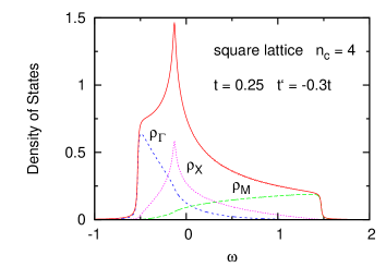
Figure 1: (Color online) Total density of states $\rho(\omega)$ and molecular orbital components $\rho_{m}(\omega)$ for four-site clusters of square lattice. For clarity, the molecular orbital components are divided by $n_{c}=4$. $\omega=0$ defines the Fermi energy for half-filling. At 14 % hole doping the van Hove singularity is shifted from $\omega=-0.13$ to $-0.09$.

Figure 1 illustrates the uncorrelated density of states components in the molecular orbital basis, where $\rho_{m}(\omega)=-\frac{1}{\pi}\,{\rm Im}\,G_{m}(\omega)$ for $\Sigma=0$, and we denote $\rho_{\Gamma}=\rho_{1}$, $\rho_{M}=\rho_{2}$, $\rho_{X}=\rho_{3,4}$. The average or local density is $\rho_{av}=(\rho_{\Gamma}+\rho_{M}+2\rho_{X})/4$. Note that all molecular orbital densities extend across the entire band width. Nevertheless, only $\rho_{X}$ contains the van Hove singularity, while $\rho_{\Gamma}$ and $\rho_{M}$ are roughly representative of the spectral weight near ${\bf k}=(0,0)$ and ${\bf k}=(\pi,\pi)$, respectively. Hole doping shifts the van Hove singularity towards $E_{F}$, whereas electron doping moves this singularity away from $E_{F}$.

A central feature of DMFT is that, to avoid double-counting of Coulomb interactions in the quantum impurity calculation, the self-energy must be removed from the small cluster in which correlations are treated explicitly. This removal yields the Green’s function

$$G_{0}(i\omega_{n})=[G(i\omega_{n})^{-1}+\Sigma(i\omega_{n})]^{-1},$$ (4)

which is also diagonal in the molecular orbital basis.

For the purpose of perfoming the ED calculation we now project the diagonal components of $G_{0}(i\omega_{n})$ onto those of a larger cluster consisting of $n_{c}=4$ impurity levels and $n_{b}=8$ bath levels. The total number of levels is $n_{s}=n_{c}+n_{b}=12$. Thus,

$$G_{0,m}(i\omega_{n}) \approx G^{cl}_{0,m}(i\omega_{n})$$ (5)

$$= \left(i\omega_{n}+\mu-\epsilon_{m}-\sum_{k=5}^{12}\frac{|V_{mk}|^{2}}{i\omega_{n}-\epsilon_{k}}\right)^{-1}$$

where $\epsilon_{m}$ denote the molecular orbital levels, $\epsilon_{k}$ the bath levels, and $V_{mk}$ the hybridization matrix elements. The incorporation of the impurity level $\epsilon_{m}$ ensures a much better fit of $G_{0,m}(i\omega_{n})$ than by projecting only onto bath orbitals.

Assuming independent baths for the cluster orbitals, each component $G_{0,m}(i\omega_{n})$ is fitted using five parameters: one impurity level $\epsilon_{m}$, two bath levels $\epsilon_{k}$ and two hopping integrals $V_{mk}$. For instance, orbital 1 couples to bath levels 5 and 9, orbital 2 to bath levels 6 and 10, etc. For the three independent cluster Green’s functions, we therefore use a total of 15 fit parameters to represent $G_{0}(i\omega_{n})$. This procedure provides a considerably more flexible projection than within a pure site basis. Since for symmetry reasons all sites are equivalent one would have in this case only four parameters (without including a level at the cluster sites). Thus, the molecular orbital basis allows for 11 additional cross hybridization terms as well as internal cluster couplings (see below). In addition, it is much more reliable to fit the three independent molecular orbital components $G_{0,m}(i\omega_{n})$ than a non-diagonal site matrix $G_{0,ij}(i\omega_{n})$ with only 4 parameters.

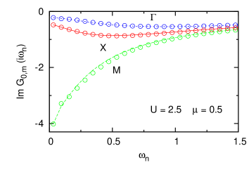
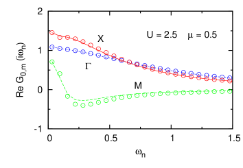
Figure 2: (Color online) Projection of lattice Green’s function components $G_{0,m}(i\omega_{n})$ onto cluster consisting of four impurity levels and eight bath levels, for $U=2.5$, $\mu=0.5$, $T=0.01$; $t^{\prime}=-0.3t$. Upper panel: Im $G_{0,m}$, lower panel: Re $G_{0,m}$. Continuous curves: diagonal elements of lattice Green’s function, Eq. (4); circles: approximate expression, right-hand side of Eq. (5).

Figure 2 illustrates the projection of the lattice Green’s function $G_{0}(i\omega_{n})$ onto the cluster for $U=2.5$ and $\mu=0.5$, which corresponds to about $\delta=0.08$ hole doping. Projections of similar quality are achieved at other Coulomb energies and chemical potentials.

The evaluation of the finite temperature interacting cluster Green’s function could in principle also be carried out in the molecular orbital basis. The Coulomb interaction then becomes a matrix containing many inter-orbital components. This step can be circumvented by using a mixed basis consisting of cluster sites $i$ and bath molecular orbitals $k$. Thus, the diagonal $8\times 8$ subblock $h_{b}=(\epsilon_{k}\delta_{kk^{\prime}})$ representing the bath levels remains unchanged, but the diagonal $4\times 4$ cluster molecular orbital submatrix now becomes nondiagonal in the cluster site basis. The transformation between sites $i$ and orbitals $m$ is given by

$$T_{im} = 0.5\left(\begin{array}[]{rrrr}1&1&1&1\\ 1&-1&-1&1\\ 1&-1&1&-1\\ 1&1&-1&-1\\ \end{array}\right).$$ (10)

In this mixed basis, the site subblock of the cluster Hamiltonian becomes

$$h_{c} = \left(\begin{array}[]{llll}\epsilon&\tau&\tau&\tau^{\prime}\\ \tau&\epsilon&\tau^{\prime}&\tau\\ \tau&\tau^{\prime}&\epsilon&\tau\\ \tau^{\prime}&\tau&\tau&\epsilon\\ \end{array}\right)$$ (15)

with $\epsilon=(\epsilon_{1}+\epsilon_{2}+2\epsilon_{3})/4$, $\tau=(\epsilon_{1}+\epsilon_{2}-2\epsilon_{3})/4$, and $\tau^{\prime}=(\epsilon_{1}-\epsilon_{2})/2$. Note that the hopping elements $t$ and $t^{\prime}$ of the original lattice Hamiltonian do not appear since they are effectively absorbed into $\tau$ and $\tau^{\prime}$ via the molecular orbital cluster levels $\epsilon_{m}$ which are adjusted to fit $G_{0,m}(i\omega_{n})$. Evidently, the procedure outlined above not only includes hopping between cluster and bath. It also introduces three new parameters within the $2\times 2$ cluster: $\epsilon$, $\tau$, and $\tau^{\prime}$. In the mixed basis, the hybridization matrix elements $V_{mk}$ between cluster and bath molecular orbitals introduced in Eq. (5) are transformed to new hybridization matrix elements between cluster sites $i$ and bath orbitals $k$. They are given by

$$V^{\prime}_{ik}=(TV)_{ik}=\sum_{m}T_{im}V_{mk}\ .$$ (16)

Thus, the upper right $4\times 8$ submatrix containing the cluster / bath hybridization matrix elements is transformed from

$$\left(\begin{array}[]{llllllll}V_{5}&0&0&0&V_{9}&0&0&0\\ 0&V_{6}&0&0&0&V_{10}&0&0\\ 0&0&V_{7}&0&0&0&V_{11}&0\\ 0&0&0&V_{8}&0&0&0&V_{12}\\ \end{array}\right)\ \ \ \$$ (21)

to

$$\left(\begin{array}[]{rrrrrrrr}V_{5}&V_{6}&V_{7}&V_{8}&\ V_{9}&V_{10}&V_{11}&V_{12}\\ V_{5}&-V_{6}&-V_{7}&V_{8}&\ V_{9}&-V_{10}&-V_{11}&V_{12}\\ V_{5}&-V_{6}&V_{7}&-V_{8}&\ V_{9}&-V_{10}&V_{11}&-V_{12}\\ V_{5}&V_{6}&-V_{7}&-V_{8}&\ V_{9}&V_{10}&-V_{11}&-V_{12}\\ \end{array}\right)\ \ \ \ \ \$$ (26)

The single-particle part of the cluster Hamiltonian then reads

$$h_{0} = \left(\begin{array}[]{ll}h_{c}&V^{\prime}\\ V^{\prime t}&h_{b}\\ \end{array}\right).$$ (29)

Adding the onsite Coulomb interactions to this hamiltonian, the non-diagonal interacting cluster Green’s function at finite $T$ can be derived from the expressionperroni ; luca

$$G^{cl}_{ij}(i\omega_{n}) = \frac{1}{Z}\sum_{\nu\mu}\,e^{-\beta E_{\nu}}\,\Big{(}\frac{\langle\nu|c_{i\sigma}|\mu\rangle\langle\mu|c_{j\sigma}^{+}|\nu\rangle}{E_{\nu}-E_{\mu}+i\omega_{n}}$$ (30)

$$\hskip 25.60747pt+\ \ \frac{\langle\nu|c_{i\sigma}^{+}|\mu\rangle\langle\mu|c_{j\sigma}|\nu\rangle}{E_{\mu}-E_{\nu}+i\omega_{n}}\Big{)}$$

where $E_{\nu}$ and $|\nu\rangle$ denote the eigenvalues and eigenvectors of the Hamiltonian, $\beta=1/T$ and $Z=\sum_{\nu}{\rm exp}(-\beta E_{\nu})$ is the partition function. At low temperatures only a small number of excited states in a few spin sectors contributes to $G^{cl}_{ij}$. They can be efficiently evaluated using the Arnoldi algorithm.arnoldi The excited state Green’s functions are computed using the Lanczos procedure. Further details are provided in Ref.perroni . The non-diagonal elements of $G^{cl}_{ij}$ are derived by first evaluating the diagonal components $G^{cl}_{ii}$ and then using the relation

$$G^{cl}_{(i+j)(i+j)}=G^{cl}_{ii}+G^{cl}_{ij}+G^{cl}_{ji}+G^{cl}_{jj}.$$ (31)

Since $G^{cl}_{ij}=G^{cl}_{ji}$, this yields:

$$G^{cl}_{ij}=\frac{1}{2}[G^{cl}_{(i+j)(i+j)}-G^{cl}_{ii}-G^{cl}_{jj}].$$ (32)

The interacting cluster Green’s function $G^{cl}_{ij}$ satisfies the same symmetry properties as $G_{ij}$ and $G_{0,ij}$. It may therefore also be diagonalized, yielding cluster molecular orbital components $G^{cl}_{m}$. The cluster molecular orbital self-energies can then be defined by an expression analogous to Eqs. (4):

$$\Sigma^{cl}_{m}(i\omega_{n})=1/G^{cl}_{0,m}(i\omega_{n})-1/G^{cl}_{m}(i\omega_{n}).$$ (33)

At real $\omega$, these cluster self-energy components, just like $G^{cl}_{0,m}$ and $G^{cl}_{m}$, have discrete spectral distributions.

The key assumption in DMFT is now that the impurity cluster self-energy is a physically reasonable representation of the lattice self-energy. Thus,

$$\Sigma_{m}(i\omega_{n})\approx\Sigma^{cl}_{m}(i\omega_{n}),$$ (34)

where, at real frequencies, $\Sigma_{m}$ is continuous.

In the next iteration step, these diagonal self-energy components are used as input in the lattice Green’s function Eq. (2), which in the molecular orbital basis is given by

$$G_{m}(i\omega_{n})=\sum_{\bf k}\left[i\omega_{n}+\mu-Tt({\bf k})T^{-1}-\Sigma(i\omega_{n})\right]^{-1}_{mm}$$ (35)

where $T$ is the transformation defined in Eq. (10). Thus, except for the diagonalization which is carried out in the mixed site / molecular orbital basis, all other steps of the calculational procedure are performed in the diagonal orbital basis. Note that $Tt({\bf k})T^{-1}$ is not diagonal at general ${\bf k}$ points. As a result, all orbital components of $\Sigma(i\omega_{n})$ contribute to each $G_{m}(i\omega_{n})$. This feature of CDMFT differs from DCA where one has a one-to-one relation between $\Sigma_{m}(i\omega_{n})$ and $G_{m}(i\omega_{n})$:maier

$$G^{\rm DCA}_{m}(i\omega_{n})=\sum_{{\bf k}_{m}}\left[i\omega_{n}+\mu-\epsilon({\bf k})-\Sigma_{m}(i\omega_{n})\right]^{-1}$$ (36)

where ${\bf k}_{m}$ labels the $m^{th}$ patch of the Brillouin zone.

The largest spin sector for $n_{s}=12$ is $n_{\uparrow}=n_{\downarrow}=6$ with dimension $N=853776$. The interacting cluster Hamiltonian matrix $h$ is extremely sparse, so that only about 20 non-zero matrix elements per row need to be stored. Since the Arnoldi algorithm requires only operations of the type $h\,u=v$, where $u,\ v$ are vectors of dimension $N$, the procedure outlined above can easily be parallelized. At temperatures of the order of $T=0.005\ldots 0.02$, one iteration takes about 15 to 60 min on 8 processors. Except near the Mott transition, 5 to 10 iterations are usually required to achieve self-consistency.

We conclude this section by pointing out that, once iteration to self-consistency has been carried out, a periodic lattice Green’s function may be constructed from the cluster components in Eq. (2) by using the superposition:parcollet

$$G({\bf k},i\omega_{n}) = \frac{1}{4}\sum_{ij=1}^{4}e^{i{\bf k}\cdot({\bf R}_{i}-{\bf R}_{j})}G_{ij}(i\omega_{n})$$ (37)

$$= G_{11}(i\omega_{n})+G_{12}(i\omega_{n})[{\rm cos}(k_{x})+{\rm cos}(k_{y})]$$

$$\ \ \ \ +\ G_{14}(i\omega_{n}){\rm cos}(k_{x}){\rm cos}(k_{y})$$

At high-symmetry points, this definition coincides with the diagonal elements introduced in Eq. (II). Thus, $G_{\Gamma}(i\omega_{n})=G((0,0),i\omega_{n})$, $G_{M}(i\omega_{n})=G((\pi,\pi),i\omega_{n})$, and $G_{X}(i\omega_{n})=G((\pi,0),i\omega_{n})=G((0,\pi),i\omega_{n})$. At ${\bf k}=(\pi/2,\pi/2)$, $G$ coincides with the onsite Green’s function $G_{11}=(G_{\Gamma}+G_{M}+2G_{X})/4$.

III Results and Discussion

III.1 Mott Transition

Figure 3 shows the occupancies of the cluster molecular orbitals $\Gamma$, $M$ and $X$ as functions of chemical potential. The average occupancy per site (both spins) is $n=(n_{\Gamma}+n_{M}+2n_{X})/2=1-\delta$, where $\delta$ is the hole doping. As revealed by the spectral distributions discussed below, the Mott transition occurs at $\mu\approx 0.7$, where the $X$ orbital becomes half-filled, whereas $n_{\Gamma}$ and $n_{M}$ approach $0.25$ and $0.75$, respectively. Thus, all three orbitals take part in the transition. This result is consistent with previous ED/DMFT calculationsal2008 for 2-site and 4-site clusters in the limit $t^{\prime}=0$, and with recent QMC results ferrero for a minimal 2-site cluster DCA version, where hole doping takes place at about the same rate for both inner and outer regions of the Brillouin zone. These trends differ, however, from results for an 8-site continuous time (CT) QMC/DCA calculationwerner which reveals initial doping primarily along the nodal direction, while near $X$ the occupancy for small $\delta$ remains at the same value as in the Mott insulator. Evidently, 2-site and 4-site cluster DMFT approaches do not provide sufficient momentum resolution to allow for ${\bf k}$-dependent doping.

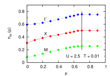
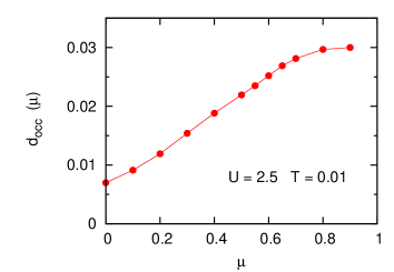
Figure 3: (Color online) Upper panel: Occupancies of cluster molecular orbitals (per spin) as functions of chemical potential $\mu$, for $U=2.5$, $T=0.01$, $t^{\prime}=-0.3t$. The Mott transition occurs at about $\mu\approx 0.7$, indicated by the vertical bar, where $n_{X}\rightarrow 0.5$, $n_{\Gamma}\rightarrow 0.75$, and $n_{M}\rightarrow 0.25$. Lower panel: Average double occupancy per site as a function of $\mu$.

The lower panel of Fig. 3 shows the average double occupancy per site. We have calculated these occupancies both for increasing and decreasing chemical potential without encountering hysteresis behavior for $T\geq 0.005$. The Mott transition induced by hole doping is therefore weakly first-order at even lower temperatures, or continuous. This result differs from the case of electron doping discussed farther below, where $n_{m}(\mu)$ as well as $d_{occ}(\mu)$ readily show hysteresis.

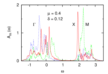
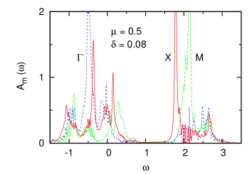
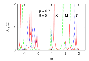
Figure 4: (Color online) Cluster spectral distributions for various chemical potentials corresponding to hole doping $\delta=0.12$, $\delta=0.08$, and $\delta=0$; $U=2.5$, $T=0.01$; broadening $\gamma=0.02$. Solid red curves: $A_{X}(\omega)$; short-dashed blue curves: $A_{\Gamma}(\omega)$, long-dashed green curves: $A_{M}(\omega)$.

To illustrate the Mott transition in the limit of half-filling, we show in Fig. 4 the spectral distributions obtained from the interacting cluster Green’s function: $A_{m}(\omega)=-(1/\pi)\,{\rm Im}\,G^{cl}_{m}(\omega+i\gamma)$, where $\gamma=0.02$. These spectra can be evaluated without requiring analytic continuation from Matsubara to real frequencies. The total density of states per spin is given by $A(\omega)=[A_{\Gamma}(\omega)+A_{M}(\omega)+2A_{X}(\omega)]/4$. All cluster molecular orbitals contribute to the spectral weight near the Fermi level in the metallic phase for $\delta>0$, and to the upper and lower Hubbard bands in the Mott phase at $\delta=0$.

The evolution of these spectra as a function of doping supports the picture conjectured long ago by Eskes et al.eskes Upon hole doping, spectral weight is transfered from the upper and lower Hubbard bands to states just above $E_{F}$, in the lower part of the Mott gap. Since the spectral weight (per spin) of both Hubbard bands initially decreases like $(1-\delta)/2$, the states induced just above $E_{F}$ have weight $\delta$ (see also Ref. phillips ). This scenario is a remarkable consequence of strong dynamical correlations and differs fundamentally from the one in ordinary semiconductors, where states induced in the gap have weight $\delta/2$ per spin for total doping $\delta$.

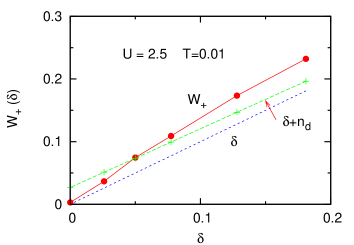
Figure 5: (Color online) Doping induced spectral weight $W_{+}(\delta)$ above $E_{F}=0$ up to about $\omega=0.9$, i.e., in the lower part of the main gap. A small constant weight is subtracted to account for the artificial broadening of the spectral peaks. This constant is chosen so that $W_{+}=0$ at $\mu=0.7$, $\delta=0$. The short-dashed blue line defines $\delta$ and the long-dashed green line $\delta+n_{d}$, where $n_{d}$ is the average double occupancy shown in Fig. 3.

Our ED/DMFT cluster calculations are in excellent agreement with this picture, as illustrated in Fig. 5 which shows the integrated spectral weight per spin induced just above $E_{F}$. This weight is denoted here as $W_{+}(\delta)$. The initial slope of $W_{+}$ is seen to be well represented by $\delta$, confirming the scenario discussed above. At finite doping $W_{+}(\delta)$ becomes even larger than $\delta+n_{d}$, where $n_{d}$ is the double-occupancy shown in Fig. 3. These results differ from those for $t^{\prime}=0$ and $T=0$ obtained by Sakai et al.sakai , who found $W_{+}(\delta)\approx\delta+n_{d}$ up to about 14 % hole doping.

Upon closer inspection, the spectral distributions shown in Fig. 4 at finite doping reveal a pseudogap close to $E_{F}$ which will be discussed in more detail in the following subsections. As shown below, this pseudogap is intimately related to the non-Fermi-liquid properties which are evident in the $X$ component of the self-energy.

III.2 Non-Fermi-Liquid Properties

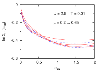
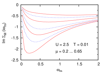
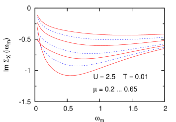
Figure 6: (Color online) Imaginary part of self-energy molecular orbital components $\Sigma_{m}(i\omega_{n})$ as functions of Matsubara frequency for various chemical potentials: $\mu=0.2,\ 0.3,\ 0.4,\ 0.5,\ 0.55,\ 0.6,\ 0.65$ (from top to bottom) corresponding to $\delta=0.24,\ 0.18,\ 0.12,\ 0.08,\ 0.05,\ 0.03,\ 0.01$, respectively; $U=2.5$, $T=0.01$.

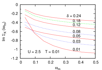
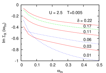
Figure 7: (Color online) Im $\Sigma_{X}(i\omega_{n})$ for various hole doping concentrations on expanded scale for $T=0.01$ (upper panel) and $T=0.005$ (lower panel). The long-dashed green curves near $\delta\approx 18$ % denote the approximate onset of non-Fermi-liquid behavior which grows until $\delta$ decreases to about 5 %.

We now discuss the low-frequency variation of the cluster self-energy which is strikingly different for the different cluster molecular orbitals. Fig. 6 shows the imaginary parts of $\Sigma_{m}(i\omega_{n})$, Eq. (34), for chemical potentials $\mu$ in the range from $0$ to $24$ % hole doping. The $\Gamma$ orbital, approximately representative of the center of the Brillouin zone, exhibits the weakest self-energy. It is nearly independent of doping and Fermi-liquid-like, with only a moderate effective mass enhancement. $\Sigma_{M}$ changes from Fermi-liquid behavior at large doping to nearly insulating behavior $\sim 1/i\omega_{n}$ close to the Mott transition. At small finite doping, it reveals strong effective mass enhancement. Both Im $\Sigma_{\Gamma}$ and Im $\Sigma_{M}$ extrapolate to very small finite values in the limit $\omega_{n}\rightarrow 0$, except near the Mott transition. In striking contrast to these orbitals, Im $\Sigma_{X}(i\omega_{n})$ exhibits a finite onset in the low-frequency limit once the doping is smaller than about $20$ % (see expanded scale in Fig. 7). The onset is largest at about $\mu=0.55$, corresponding to $\delta=5$ %. At smaller doping (larger $\mu$), i.e., very close to the Mott transition, it diminishes again.

In addition to the low-frequency onset of Im $\Sigma_{X}(i\omega_{n})$ which gives rise to reduced quasiparticle lifetime, the non-Fermi-liquid behavior also leads to a characteristic flattening of Im $\Sigma_{X}(i\omega_{n})$, which induces a sharp resonance in Im $\Sigma_{X}(\omega)$ at small positive frequencies. As will be discussed in the next subsection, it is this resonance that is responsible for the pseudogap in the density of states.

Similar results are obtained at lower temperature, $T=0.005$, as shown in the lower panel of Fig. 7. Again, the largest deviation from Fermi-liquid behavior is found for Im $\Sigma_{X}(i\omega_{n})$ at about $6$ % doping. The onset of non-Fermi-liquid properties occurs at slightly smaller doping than for $T=0.01$. The results shown in Figs. 6 and 7 are consistent with the $T=0$  ED/CDMFT calculations by Civelli et al.civelli

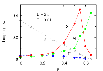
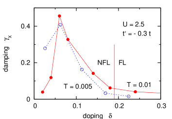
Figure 8: (Color online) Upper panel: Low-frequency damping rates $\gamma_{m}=-{\rm Im}\,\Sigma_{m}(i\omega_{n}\rightarrow 0)$ as functions of chemical potential. Solid red curves: $X$ orbital, short-dashed blue curves: $\Gamma$ orbital, long-dashed green curves: $M$ orbital. The dotted curve denotes the doping $\delta$ (same scale as $\gamma_{m}$); $U=2.5$, $T=0.01$. For $\mu>0.2\ldots 0.3$ or $\delta<0.18\ldots 0.20$, $\gamma_{X}$ increases strongly, indicating the onset of non-Fermi-liquid behavior. Lower panel: comparison of $\gamma_{X}$ as a function of doping for $T=0.01$ (solid red circles) and $T=0.005$ (empty blue circles). The vertical bar denotes the approximate location of the transition from Fermi-liquid to non-Fermi-liquid behavior.

To illustrate this non-Fermi-liquid behavior of $\Sigma_{X}$ in more detail, we compare in the upper panel of Fig. 8 the low-frequency limits $\gamma_{m}\equiv-{\rm Im}\,\Sigma_{m}(i\omega_{n}\rightarrow 0)$ as functions of chemical potential. These values were found to be nearly the same for a linear extrapolation from the first two Matsubara points and for a quadratic fit using the first three points. At $\mu>0.3$ or $\delta<0.18$, $\gamma_{X}$ increases strongly, indicating the onset of a non-Fermi-liquid phase. The lower panel shows the variation of $\gamma_{X}$ with doping for $T=0.01$ and $T=0.005$. At lower $T$, the onset of non-Fermi-liquid behavior is seen to be slightly sharper and to shift to slightly lower $\delta$.

At finite temperature, a sharp transition between Fermi-liquid and non-Fermi-liquid phases is not to be expected. According to the detailed temperature variation of the self-energy of the two-dimensional Hubbard model studied recently by Vidhyadhiraja et al.vidhya within QMC/DCA for $4\times 4$ clusters ($U=1.5$, $t^{\prime}=0$), a quantum critical point exhibiting marginal Fermi-liquid behavior was found at $\delta_{c}\approx 15$ % doping, with Fermi-liquid behavior at larger $\delta$ and a pseudogap phase at $\delta<\delta_{c}$. At $T=0.01$, the $T$ / $\delta$ phase diagram indicates a crossover region of about $\delta=0.15\pm 0.02$ between these phases. Assuming a crossover region of similar width, i.e., $\Delta\delta\approx 0.04$, the results shown in Fig. 8 are consistent with those of Ref.vidhya . Thus, for $U=2.5$, $t^{\prime}=-0.3t$, the Fermi-liquid and non-Fermi-liquid phases seem to be separated by a quantum critical point at $\delta_{c}\approx 18\ldots 20$ %, with marginal Fermi-liquid behavior for $T\geq 0$.

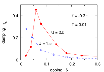
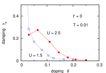
Figure 9: (Color online) Low-frequency damping rate of $X$ orbital, $\gamma_{X}=-{\rm Im}\,\Sigma_{X}(i\omega_{n}\rightarrow 0)$ as a function of doping for various Coumb energies and next-nearest-neighbor hopping energies; $T=0.01$. Upper panel: $t^{\prime}=-0.3t$, lower panel: $t^{\prime}=0$. Solid red circles: $U=2.5$, empty blue circles: $U=1.5$.

Figure 9 compares the low-frequency damping rate of the $X$ orbital as a function of doping for $U=2.5$ and $U=1.5$. The upper panel shows the results for $t^{\prime}=-0.3t$, the lower panel for $t^{\prime}=0$. The case $U=1.5$, $t^{\prime}=0$ suggests a critical doping $\delta_{c}\approx 0.15\pm 0.02$, in agreement with the results of Ref. vidhya . As is to be expected, at smaller $U$ $\delta_{c}$ is smaller than at large $U$, since the Fermi liquid properties are stabilized. A similar trend occurs as $t^{\prime}$ is shifted from $t^{\prime}=-0.3t$  to  $t^{\prime}=0$. Nevertheless, despite the large variations in $U$ and $t^{\prime}$, the critical doping separating the Fermi-liquid and non-Fermi-liquid phases is remarkably stable and occurs in the range $\delta_{c}\approx 0.15\ldots 0.20$, i.e., close to the optimal doping concentrations found in many high-$T_{c}$ cuprates.

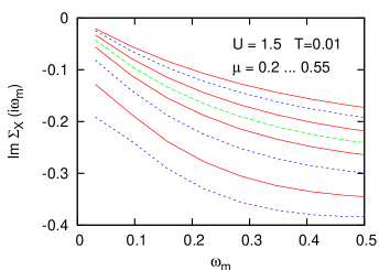
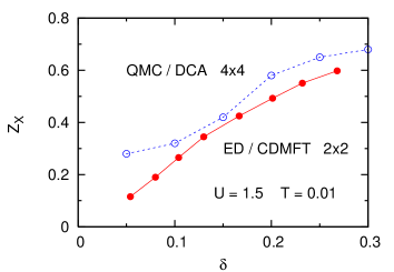
Figure 10: (Color online) Upper panel: imaginary part of $\Sigma_{X}(i\omega_{n})$ as a function Matsubara frequency for $\mu=0.2\ldots 0.55$ in steps of $0.05$ (from top), for $U=1.5$, $t^{\prime}=0$, $T=0.01$. $\mu=0.3$ (long-dashed green curve) corresponds to $\delta=0.18$ and approximately marks the transition from Fermi-liquid to non-Fermi-liquid behavior. Lower panel: Solid red circles: $Z_{X}=1/(1-{\rm Im}\Sigma_{X}(i\omega_{0})/\omega_{0})$ derived from ED/CDMFT results in upper panel; empty blue circles: analogous QMC/DCA results from Fig. 1 of Ref. vidhya for $T=0.014$.

For a more detailed comparison with the results of Ref. vidhya , we show in Fig. 10 the variation of Im $\Sigma_{X}(i\omega_{n})$ with chemical potential for $U=1.5$, $t^{\prime}=0$ and $T=0.01$. These values of $\mu$ correspond to dopings in the range $\delta=0.27\ldots 0.05$. Although the overall magnitude of Im $\Sigma_{X}$ is much smaller than in Fig. 7 for $U=2.5$, $t^{\prime}=-0.3t$, there is again a clear separation between doping larger than $\delta_{c}\approx 0.17$ exhibiting Fermi-liquid behavior, and smaller doping with characteristic non-Fermi-liquid features. The lower panel shows the comparison of the approximate quasiparticle weight, $Z_{X}=1/[1-{\rm Im}\Sigma_{X}(i\omega_{0})/\omega_{0}]$, derived from the ED/DMFT results in the upper panel, with the corresponding QMC/DCA values taken from Fig. 1 of Ref. vidhya . For $\delta>0.15$ the agreement is very good. (Note that for $Z_{X}>0.5$, $-{\rm Im}\,\Sigma_{X}(i\omega_{0})$ is less than $\omega_{0}=0.031$.) At smaller doping, the difference becomes larger, presumably because of the finer momentum resolution achieved for the $4\times 4$ cluster in Ref. vidhya .

To analyze the difference between CDMFT and DCA for $2\times 2$ clusters, with identical system parameters, we compare in Fig. 11 the low-frequency damping rate of $\Sigma_{X}(i\omega_{n})$ as a function of doping. Evidently, the different relations between self-energy components $\Sigma_{m}$ and lattice Green’s function $G_{m}$ in these two schemes give rise to changes on a quantitative level. Nevertheless, both approaches predict a transition from a Fermi-liquid phase at hole doping larger than about 20 % to a non-Fermi-liquid phase at small doping. Surprisingly, the transition is less sharp in DCA than in CDMFT. The reason for this difference might be that, in contrast to CDMFT, the momentum patches of the Brillouin zone are not coupled in the evaluation of the DCA lattice Green’s function (see Eq. (36)). It might therefore be necessary in DCA to treat larger clusters (such as $8$ siteswerner or $16$ sitesvidhya ) in order to obtain a sharper Fermi-liquid to non-Fermi-liquid transition. A slower convergence with cluster size in DCA is also found for the critical Coulomb energy at half filling.gull ; werner

III.3 Pseudogap

The non-Fermi-liquid properties of $\Sigma_{X}(i\omega_{0})$ manifest themselves not only in the enhanced low-frequency damping rate discussed above, but also in the flattening of Im $\Sigma_{X}(i\omega_{n})$ which can be identified as the origin of the pseudogap in the density of states. Narrow gaps near $E_{F}$ below the critical doping are already evident in the cluster spectra shown in Fig. 4. Fig. 12 shows these spectra on an expanded scale for $\delta=\delta_{c}\approx 0.18$ and $\delta=0.03$. While near critical doping the density of states is Fermi-liquid-like, with a sharp peak at $E_{F}$, smaller hole doping leads to a very asymmetric density of states, with a pseudogap of magnitude $\Delta\approx 4t^{2}/U=0.1$ right above $E_{F}$. The molecular orbital analysis of these spectra reveals that this pseudogap is associated entirely with the $A_{X}(\omega)$ contribution, i.e., with scattering processes involving momenta close to $(\pi,0)$ and $(0,\pi)$. With decreasing doping, the peak at $E_{F}$ seen for $\delta\approx\delta_{c}$ shifts downwards, so that the Fermi level gradually moves into the pseudogap. At the same time, the pseudogap becomes wider and the spectral weight above $E_{F}$ is reduced until the transition to the Mott phase occurs at half filling. (The peak at $\omega\approx 0.25$ for $\delta=0.18$ is due to the discreteness of the cluster spectra and is not related to the pseudogap. The actual pseudogap at this large doping is vanishingly small; see analysis of self-energy below).

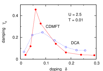
Figure 11: (Color online) Comparison of low-frequency damping rate of $X$ orbital, $\gamma_{X}=-{\rm Im}\,\Sigma_{X}(i\omega_{n}\rightarrow 0)$ as a function of doping for CMDFT (solid red circles) and DCA (empty blue circles); $U=2.5$, $T=0.01$.

Note that the peak at $E_{F}$ for $\delta=\delta_{c}$ is also compatible with marginal Fermi-liquid behavior. Finite-size effects, however, do not permit a clear distinction between Fermi-liquid properties below the first Matsubara frequency $\omega_{0}$ and genuine marginal Fermi-liquid behavior at $\delta_{c}$.vidhya

The lower panel of Fig. 12 shows the corresponding spectra derived from the lattice Green’s function components $G_{m}(i\omega_{n})$, Eq. (35), via extrapolation to real $\omega$. Thus, $A(\omega)=-\frac{1}{\pi}{\rm Im}\,[G_{\Gamma}(\omega)+G_{M}(\omega)+2G_{X}(\omega)]/4$. We use here the routine ratint.ratint Nearly identical spectra are obtained via Padé extrapolation. About $400\ldots 600$ Matsubara points are taken into account for the energy window $-1\leq\omega\leq 1$, and the same broadening is assumed ($\gamma=0.02$) as in the cluster spectra shown in the upper panel. As a result of the accurate self-energies and Green’s functions along the Matsubara axis, the extrapolation to low real $\omega$ is highly reliable. The lattice spectra confirm the trend observed in the cluster spectra: At $\mu=0.3$, $\delta=0.18$, the density of states has a peak very close to the Fermi level, while for $\mu=0.6$, $\delta=0.03$, $E_{F}$ lies in a pseudogap of about the same width as in the cluster data. The lattice spectra $A(\omega)$ can also be calculated by first extrapolating the self-energy components $\Sigma_{m}(i\omega_{n})$ to real frequencies and then using Eq. (35) at real $\omega$. The results are fully consistent with the spectra derived via extrapolation of $G_{m}(i\omega_{n})$.

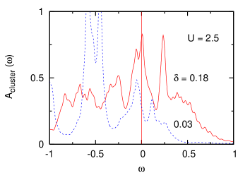
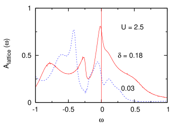
Figure 12: (Color online) Upper panel: Cluster spectral distributions $A(\omega)=\frac{1}{4}[A_{\Gamma}(\omega)+A_{M}(\omega)+2A_{X}(\omega)]$ for $U=2.5$, $t^{\prime}=-0.3t$, $T=0.01$. Solid red curve: $\mu=0.3$ (hole doping $\delta=0.18$) with peak at $E_{F}=0$; dashed blue curve: $\mu=0.6$ ($\delta=0.03$) exhibiting a pseudogap above $E_{F}$; lower panel: analogous lattice spectra obtained via extrapolation of Green’s function components, Eq. (35).

The pseudogap seen in Fig. 12 for $\delta=0.03$ is reminiscent of the pseudogap obtained in the two-band model within local DMFT above the first Mott transition.prb04 Once the electrons in the narrow subband are Mott localized, an effective two-fluid system is realized in which the Coulomb interaction with the remaining conduction electrons generates deviations from Fermi-liquid behavior, in particular, the finite lifetime associated with the low-frequency limit of ${\rm Im}\,\Sigma(i\omega_{n})$, and the characteristic flattening of this function which gives rise to a pseudogap at real $\omega$.al+costi This two-band model exhibits a quantum critical point when the pseudogap turns into the Mott gap.costi It would be interesting to inquire whether the present cluster picture of the single band model could be mapped onto this two-band model. The spatial degrees of freedom in the cluster would then play the role of the inter-orbital fluctuations in the two-band model. Since at small hole doping a sizable number of electrons is Mott localized their spins act as scattering centers for the remaining electrons whose self-energy then exhibits deviations from Fermi-liquid behavior.

To illustrate the effect of non-Fermi-liquid behavior on the self-energy at real $\omega$, we show in Fig. 13 the low-frequency variation of Im $\Sigma_{X}(\omega)$ obtained from the lower panel of Fig. 7 via extrapolation to real $\omega$. Typically, at these low frequencies we use the first $100\ldots 400$ Matsubara points and evaluate Im $\Sigma_{X}$ at $\omega+i\gamma$, with $\gamma=0.005$. Although the details of the resulting spectra differ slightly, the important qualitative features near $E_{F}$ are very stable. Spectra derived via Padé extrapolation are very similar.

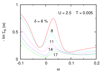
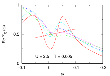
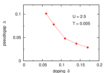
Figure 13: (Color online) Self-energy $\Sigma_{X}(\omega)$ obtained via extrapolation to real frequencies for several hole doping concentrations (broadening $\gamma=0.005$). Upper panels: $-$Im $\Sigma_{X}$ and Re $\Sigma_{X}$; $U=2.5$, $T=0.005$. The outer intersections of Re $\Sigma_{X}$ with the straight lines $\omega+\mu-\epsilon_{k}$ yield the approximate width of the pseudogap $\Delta$. Lower panel: Pseudogap $\Delta$ as a function of hole doping derived from self-energies $\Sigma_{X}(\omega)$ shown in upper panels.

As can be seen in Fig. 13, at large hole doping $-$Im $\Sigma_{X}(\omega)$ has a minimum at $E_{F}$ and varies quadratically at small $\omega$, as expected for a Fermi liquid. Damping in this range is very weak. Nevertheless, even for $\delta\geq 0.17$ a small peak in $-$Im $\Sigma_{X}(\omega)$ is found at about $\omega=0.05$ above $E_{F}$, indicating that electrons added to the system just above $E_{F}$ have a reduced lifetime. With decreasing doping, this feature grows into a strong resonance which eventually dominates the low-frequency properties. The minimum of $-$Im $\Sigma_{X}(\omega)$ is then shifted slightly below $E_{F}$ and a second minimum appears above $E_{F}$. Moreover, this resonance shows a dispersion as a function of doping. It first shifts downwards from $\omega\approx 0.05$ to $0.02$ and then disperses again upwards to about $\omega\approx 0.05$. Re $\Sigma_{X}(\omega)$ is seen to exhibit a positive slope at the resonance which is consistent with Kramers-Kronig relations. This implies that spectral weight is removed from the resonance region where correlation induced damping is large.

The evolution of the resonance in Im $\Sigma_{X}(\omega)$ with doping is one of the main results of this work and has to our knowledge not been discussed previously. A weak resonance in Im $\Sigma_{X}$ at $5$ % doping was also found by Jarrell et al.jarrell2001 within QMC/DCA for $n_{c}=4$. The fact that this resonance is much stronger in the present results might be related to the faster convergence of CDMFT with cluster size (see discussion of Fig. 11). A resonance in Im $\Sigma(\omega)$ is also obtained in the spectral weight transfer model proposed by Philipps et al.phillips In this scheme, however, the resonance is located at $\omega=0$ independently of doping.

The outer intersections of Re $\Sigma_{X}(\omega)$ with $\omega+\mu-\epsilon_{k}$ provide the approximate width of the pseudogap $\Delta$ in the spectral distribution. The central intersection does not yield any peak because of the short lifetime in this frequency range. The new minima of $-$Im $\Sigma_{X}(\omega)$ below and above the resonance are consistent with the spectral peaks just below and above $E_{F}$, as seen in the results for $\delta=0.03$ in Fig. 12. For increasing hole doping, the resonance of Im $\Sigma_{X}(\omega)$ becomes weaker so that for $\delta>0.17$ there are no longer three intersections of $\omega+\mu-\epsilon_{k}$ with Re $\Sigma_{X}(\omega)$. The pseudogap then vanishes. At smaller doping, the peak in $-$Im $\Sigma_{X}(\omega)$ grows and the pseudogap gets wider. This trend, however, is superceded by the reduction of spectral weight above $E_{F}$ as the Mott transition at half-filling is approached.

The lower panel of Fig. 13 shows the approximate width of the pseudogap $\Delta$. We use here the outer intersections of Re $\Sigma_{X}(\omega)$ with the lines $\omega+\mu-\epsilon_{k}$ to define the magnitude of $\Delta$, where $\epsilon_{k}$ is chosen so that $\omega+\mu-\epsilon_{k}$ passes through the inflection point in the region of the maximal positive slope of Re $\Sigma_{X}(\omega)$. Other values of $\epsilon_{k}$ yield similar values of $\Delta$. In the spectral distributions, this definition of the pseudogap roughly corresponds to the peak-to-peak separation of spectral weight near the gap. Systematically smaller values of $\Delta$ are obtained, for instance, if the width of the gap half-way between the minimum of $A(\omega)$ and the neighboring maxima is chosen as definition. At $\delta>0.17$, the definition used above no longer yields a pseudogap and the system turns into an ordinary Fermi liquid.

The doping dependent resonance in Im $\Sigma_{X}(\omega)$ and the concomitant opening of the pseudogap are consistent with recent angle-resolved photoemission (ARPES) data by Yang et al. yang3 According to the upper panel of Fig. 13, for $\delta\geq 0.17$ the quasiparticle damping is symmetric for electron and hole states. Below this doping, the lifetime of electron states above $E_{F}$ is much shorter than that of hole states below $E_{F}$, giving rise to the opening of the pseudogap above $E_{F}$ and the striking particle-hole asymmetry observed in the data. Moreover, the results shown in Fig. 13 are specific to the $(\pi,0)$ component of the self-energy and are absent in $\Sigma_{\Gamma}(\omega)$ and $\Sigma_{M}(\omega)$. Thus, the particle-hole asymmetry and pseudogap above $E_{F}$ are momentum dependent features which are most pronounced in the antinodal region, but weak or absent along the nodal $\Gamma M$ direction which also agrees with the experimental data. yang3 A more detailed discussion of the momentum variation of the self-energy will be given in the final subsection.

Because of the finite temperature in the ED/CDMFT calculation, it is not possible to identify spectral features at frequencies below the first Matsubara point ($\omega_{0}=0.0314$ for $T=0.01$). Nevertheless, the doping variation of the pseudogap shown in Fig. 13 is found to be robust. In particular, it is clear that the pseudogap is directly linked to the resonance in $-$Im $\Sigma_{X}(\omega)$ which, in turn, reflects the non-Fermi-liquid properties of the system. Since for $\delta>\delta_{c}$ ordinary Fermi-liquid behavior is established, it is evident that the pseudogap then vanishes.

The above scenario is consistent with the fact that for a hole-doped Mott insulator the addition of electrons pushes the system closer to the insulating phase. This implies that spectral weight just above $E_{F}$ must be removed and shifted towards the upper and lower Hubbard bands. This is precisely the effect induced via the large damping associated with the low-frequency resonance in $-$Im $\Sigma_{X}(\omega)$ and the positive slope of Re $\Sigma_{X}(\omega)$.

According to this picture, the creation of holes in an electron-doped Mott insulator also moves the system closer to the insulating phase. Thus, spectral weight from states just below $E_{F}$ must be shifted to the Hubbard bands. As discussed in the next subsection, the ED/CDMFT results confirm this prediction. The $X$ component of the self-energy along the Matsubara axis again exhibits non-Fermi-liquid behavior at sufficiently low electron doping. The extrapolation to real $\omega$, however, now reveals a resonance slightly below $E_{F}$, rather than above $E_{F}$ as for hole doping.

III.4 Electron Doping

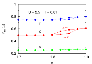
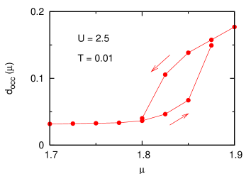
Figure 14: (Color online) Upper panel: Occupancies of cluster molecular orbitals (per spin) as functions of chemical potential $\mu$, for $U=2.5$, $T=0.01$. For electron doping, the Mott transition occurs at about $\mu\approx 1.8\ldots 1.875$. In the insulating phase $0.7<\mu<1.8$, $n_{X}=0.5$, $n_{\Gamma}=0.75$, and $n_{M}=0.25$ (see also Fig. 3). The arrows denote the hysteresis behavior for increasing vs. decreasing $\mu$. Lower panel: Average double occupancy per site as a function of $\mu$.

For completeness we discuss in this subsection the case of electron doping which differs from hole doping because of the second-neighbor hopping term $t^{\prime}$. As a result of this interaction, the density of states shown in Fig. 1 is asymmetric, so that electron doping shifts the van Hove singularity away from $E_{F}$ rather than towards it. Thus, the density of states is reduced and less steep. Fig. 14 shows the occupancies of the cluster molecular orbitals in the vicinity of the Mott transition induced via electron doping. Both these occupancies as well as the double occupancy shown in the lower panel exhibit hysteresis behavior for increasing vs. decreasing chemical potential, indicating that this transition is first order. Thus, this transition is similar to the doping-induced metal insulator transitions found within local DMFT for single-band and multi-band stystems. kotliar:doping ; garcia ; al:doping

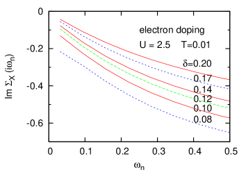
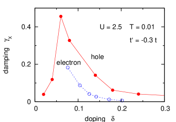
Figure 15: (Color online) Upper panel: Imaginary part of $\Sigma_{X}(i\omega_{n})$ as a function Matsubara frequency for electron doping; $U=2.5$, $t^{\prime}=-0.3t$, $T=0.01$. The long-dashed green curve for $\delta=0.12$ approximately marks the transition from Fermi-liquid to non-Fermi-liquid behavior. The corresponding self-energy for hole doping is shown in Fig. 7. Lower panel: Comparison of damping $\gamma_{X}=-{\rm Im}\,\Sigma_{X}(i\omega_{n}\rightarrow 0)$ for hole doping (solid red circles) and electron doping (empty blue circles).

Because of the lower and less steep density of states for electron doping, the low-frequency variation of the self-energy differs greatly from the hole doping case, as illustrated in Fig. 15. Although there is again a clear distinction between Fermi-liquid and non-Fermi-liquid behavior, the transition now occurs at considerably smaller $\delta$. While for hole doping $\delta_{c}\approx 0.18\ldots 0.20$, for electron doping we find $\delta_{c}\approx 0.12$. Thus, the Fermi-liquid phase is stabilized.

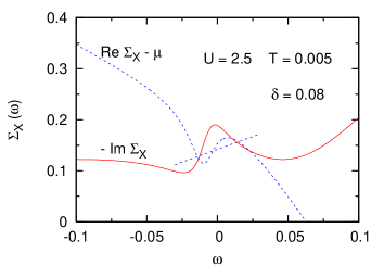
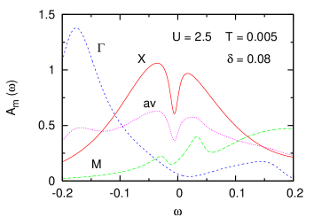
Figure 16: (Color online) Upper panel: real and imaginary parts of $\Sigma_{X}(\omega)$ for electron doping obtained via extrapolation to real $\omega$. The intersections of Re $\Sigma_{X}(\omega)-\mu$ with $\omega-\epsilon_{k}$ (straight line) provide the pseudogap. Lower panel: spectral distributions derived via extrapolation of lattice Green’s function components $G_{m}(i\omega_{n})$ to real $\omega$. The average density corresponds to $A(\omega)=-\frac{1}{4\pi}{\rm Im}\,[G_{\Gamma}(\omega)+G_{M}(\omega)+2G_{X}(\omega)]$.

To identify the pseudogap for electron doping, we evaluate the cluster self-energy components via extrapolation to real frequencies. The upper panel of Fig. 16 shows $\Sigma_{X}(\omega)$ at small $\omega$. In this case the non-Fermi-liquid properties give rise to a resonance in $-$Im $\Sigma_{X}(\omega)$ centered slightly below the Fermi level, indicating that the creation of hole states in an electron-doped Mott insulator implies a transfer of spectral weight from states near $E_{F}$ to the Hubbard bands. Thereby the system is brought closer to the insulating phase. Accordingly, the real part of $\Sigma_{X}(\omega)$ exhibits a positive slope close to $E_{F}$. Its intersections with $\omega+\mu-\epsilon_{k}$ can be used to define the pseudogap. For $\delta=0.08$ the gap is found to be $\Delta\approx 0.03$, i.e., only about half as large as for the hole doping case shown in Fig. 13. The lower panel of Fig. 16 shows the quasiparticle distributions obtained via extrapolation of the lattice Green’s function components, Eq. (35), to real $\omega$. The dominant feature at small $\omega$ is the pseudogap in the $X$ component, which is consistent with the behavior of $\Sigma(\omega)$ displayed in the upper panel.

The main difference with respect to hole doping, apart from the smaller size of the pseudogap, is the fact that this gap can be identified only in a very narrow doping range. At electron doping larger than $0.08$, the non-Fermi-liquid behavior is quickly replaced by ordinary Fermi-liquid properties. At smaller doping, spectral weight just below $E_{F}$ is rapidly transferred to the Hubbard bands, so that the pseudogap is superceded by the opening on the Mott gap.

III.5 Phase Diagram

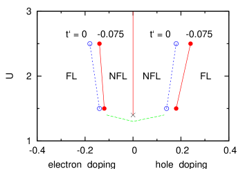
Figure 17: (Color online) Phase diagram of two-dimensional Hubbard model calculated within ED/CDMFT for $2\times 2$ clusters. The Fermi-liquid phase at large hole or electron doping is turned into a non-Fermi-liquid phase at small doping. The symbols for $U=1.5$ and $U=2.5$ indicate the approximate critical doping $\delta_{c}$ for $t^{\prime}=-0.075$ (solid red circles) and for $t^{\prime}=0$ (empty blue circles). The vertical line at $\delta=0$ marks the Mott phase at half-filling. The critical $U$ indicated by $\times$ is about $1.4$ for $t^{\prime}=0$ and $t^{\prime}=-0.3t$. The long-dashed green line denotes the approximate lower bound of the non-Fermi-liquid domain.

In Figure 9 we have shown that the onset of non-Fermi-liquid behavior is shifted to smaller hole doping when $U=2.5$ is reduced to $U=1.5$ and when $t^{\prime}=-0.3t$ is replaced by $t^{\prime}=0$. Fig. 15 illustrates the reduction of $\delta_{c}$ for $U=2.5$ when hole doping is replaced by electron doping. A similar reduction is found for $U=1.5$ (not shown). In Fig. 17 we collect these data and display the phase diagram of the present Hubbard model for electron and hole doping. At finite temperature the values of $\delta_{c}$ can only be determined within an accuracy of about $\pm 0.02$. For clarity, these margins are not plotted in Fig. 17. Despite this uncertainty, the results demonstrate several trends: for hole doping $\delta_{c}$ diminishes with decreasing $U$ and when $t^{\prime}=-0.3t$ is replaced by $t^{\prime}=0$. Moreover, for $t^{\prime}=-0.3t$ the critical doping decreases when hole doping is replaced by electron doping. As pointed out above, the variation of $\delta_{c}$ is surprisingly small, despite the rather large changes in $U$ and $t^{\prime}$.

III.6 Momentum Variation

According to the results shown in Fig. 6 the non-Fermi-liquid properties of the two-dimensional Hubbard model at low hole doping are mainly associated with the $X$ component of the self-energy. Only very close to the Mott transition the $M$ component begins to dominate since its imaginary part changes from $\sim\omega_{n}$ to $\sim 1/\omega_{n}$. The cluster components of the self-energy may be used to construct an approximate momentum dependent lattice self-energy by using the same periodization as in Eq. (37) for the Green’s function. Thus, civelli

$$\Sigma({\bf k},\omega)=\alpha_{\Gamma}({\bf k})\Sigma_{\Gamma}(\omega)+\alpha_{M}({\bf k})\Sigma_{M}(\omega)+\alpha_{X}({\bf k})\Sigma_{X}(\omega)$$ (38)

where

$$\alpha_{\Gamma}({\bf k}) = [1+{\rm cos}k_{x}][1+{\rm cos}k_{y}]/4$$

$$\alpha_{M}({\bf k}) = [1-{\rm cos}k_{x}][1-{\rm cos}k_{y}]/4$$ (39)

$$\alpha_{X}({\bf k}) = [1-{\rm cos}k_{x}{\rm cos}k_{y}]/2.$$

The ${\bf k}$-resolved spectral distributions are then given by

$$A({\bf k},\omega)=-\frac{1}{\pi}{\rm Im}\,(\omega+\mu-\epsilon({\bf k})-\Sigma({\bf k},\omega))^{-1}.$$ (40)

An alternative is to periodize instead the cumulant matrixstanescu2 $M(\omega)=1/[\omega+\mu-\Sigma(\omega)]$ which can be diagonalized in the same manner as the self-energy. Thus, the molecular orbital components of $M(\omega)$ are given by $M_{m}(\omega)=1/[\omega+\mu-\Sigma_{m}(\omega)]$ and the momentum dependent lattice cumulant $M({\bf k},\omega)$ can be derived from an expression analogous to Eq. (38)

$$M({\bf k},\omega)=\alpha_{\Gamma}({\bf k})M_{\Gamma}(\omega)+\alpha_{M}({\bf k})M_{M}(\omega)+\alpha_{X}({\bf k})M_{X}(\omega).$$ (41)

The lattice self-energy in this approximation takes the form

$$\Sigma({\bf k},\omega)=\omega+\mu-1/M({\bf k},\omega).$$ (42)

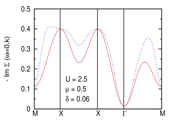
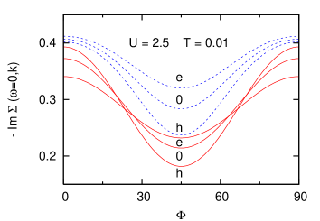
Figure 18: (Color online) Upper panel: momentum variation of imaginary part of $-\Sigma_{X}(\omega,{\bf k})$ at Fermi level. Solid red curve: expression Eq. (38), corresponding to periodization of cluster self-energy; dashed blue curve: expression Eq. (42), corresponding to periodization of cumulant; $U=2.5$, $\delta=0.06$, $T=0.01$. Lower panel: azimuthal variation of $-$Im $\Sigma_{X}(\omega=0,{\bf k})$ for ${\bf k}=\pi(1-r{\rm sin}\Phi,1-r{\rm cos}\Phi)$ with $r=0.7,\ 0.8,\ 0.9$, approximately representing electron doping (e), half-filling (0), and hole doping (h), respectively. $\Phi=0,90$ corresponds to ${\bf k}$ along $XM$ and $\Phi=45$ to the nodal direction $\Gamma M$. Solid red curves: periodization via Eq. (38); dashed blue curves: periodization via Eq. (42).

In the upper panel of Fig. 18 we compare these two versions of $\Sigma({\bf k},\omega)$ at $\omega=0$ for $\delta=0.06$ hole doping. The real-$\omega$ components $\Sigma_{m}(\omega=0)$ are obtained via extrapolation from the first few Matsubara frequencies. At high-symmetry points both versions of Im $\Sigma({\bf k},\omega=0)$ coincide. At general ${\bf k}$-points, however, the cumulant expression yields enhanced damping, in particular, between $M$ and $X$, and along $\Gamma M$. The enhancement near $X$ leads to an effective flattening of Im $\Sigma({\bf k},\omega)$, which is also seen in the dual Fermion approach.rubtsov On the other hand, it is not clear whether this enhancement is partly an artifact of the cumulant approximation since the damping at some points between $X$ and $M$ is even larger than at $X$. Also, damping near ${\bf k}\approx 2/3(\pi,\pi)$ in the cumulant version is almost as large as at $X$. At the present doping ($\delta=0.06$), the periodization of the self-energy according to Eq. (38) is in better agreement with the dual Fermion approach (see Fig. 15 of Ref. rubtsov ).

The lower panel of Fig. 18 shows the variation of $-$Im $\Sigma(\omega=0,{\bf k})$ along ${\bf k}=\pi(1-r{\rm sin}\Phi,1-r{\rm cos}\Phi)$ where $r=0.7,\ 0.8,\ 0.9$ is chosen to approximately represent the Fermi arcs for electron doping, half-filling, and hole doping, respectively. Both periodization versions yield consistently larger damping along $XM$ than along the nodal direction $\Gamma M$. The cumulant version implies overall larger damping, and, more importantly, less pronounced difference between $\Gamma M$ and $XM$. Because of the substantial imaginary part of the self-energy at low frequencies, the Fermi surface in the present $2\times 2$ cluster approach exhibits arcs rather than hole pockets.civelli We note, however, that greater momentum differentiation obtained for larger clusters might lead to more pronounced anisotropy between the nodal and anti-nodal directions. In particular, this could yield smaller values of $-$Im $\Sigma(\omega=0,{\bf k})$ along $\Gamma M$ ($\Phi=45$) than indicated in Fig. 18.

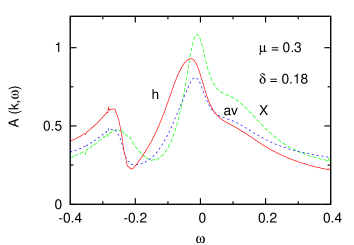
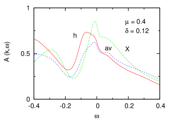
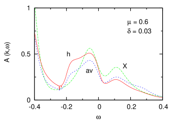
Figure 19: (Color online) Lattice spectral distributions $A({\bf k},\omega)$ for three chemical potentials close to critical doping ($\mu=0.3$, upper panel), incipient pseudogap formation ($\mu=0.4$, middle panel), and complete pseudogap phase ($\mu=0.6$, lower panel). Solid red curves ($h$): $k_{x}=k_{y}=0.36\pi$ near Fermi surface for hole doping; dashed blue curves ($av$): $k_{x}=k_{y}=0.5\pi$ at center of Brillouin zone, corresponding to average density; long-dashed green curves ($X$): ${\bf k}=(\pi,0)=X$; $U=2.5$, $T=0.01$.

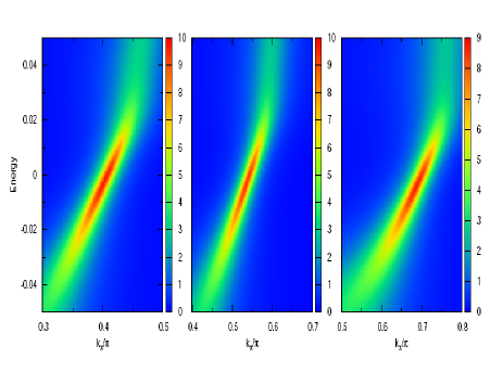
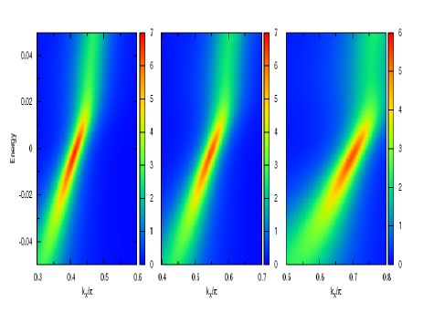
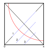
Figure 20: (Color online) Upper three panels: Spectral function $A({\bf k},\omega)$ along cuts 1, 2, 3 (from left to right); top panel: doping $\delta=0.17$; middle panel: $\delta=0.14$; $U=2.5$, $T=0.005$. Lower panel: Cuts through Brillouin zone corresponding to ARPES data in Ref.yang3 . Solid red curve: approximate non-interacting Fermi surface for hole doping.

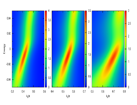
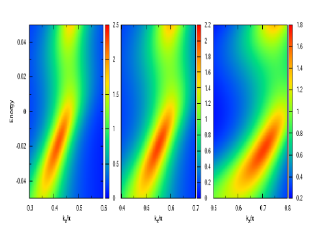
Figure 21: (Color online) Same as Fig. 20 except $\delta=0.11$ (upper panel) and $\delta=0.08$ (lower panel).

According to the collective mode in Im $\Sigma_{X}(\omega=0)$ (see Fig. 13), the anisotropy between the $\Gamma X$ and $\Gamma M$ directions is even larger above $E_{F}$ than for the $\omega\rightarrow 0$ limit shown in Fig. 18. Thus, the collective mode gives rise to a momentum and doping dependent particle-hole asymmetry. To illustrate this point, we show in Fig. 19 the low-frequency part of the spectral distribution $A({\bf k},\omega)$, derived via extrapolation of the lattice Green’s function, Eq. (37), at three representative points in the Brillouin zone. Three doping regions can be distinguished: At $\mu=0.3$ close to optimal doping ($\delta=0.18$, upper panel), there is weak anisotropy since the system is a Fermi liquid throughout ${\bf k}$ space. Below critical doping ($\mu=0.4$, $\delta=0.12$, middle panel), the spectrum in the anti-nodal direction at $X$ shows clear signs of pseudogap behavior, while the one at ${\bf k}=0.36(\pi,\pi)$, i.e., near the nodal point of the Fermi surface for hole hoping, is still dominated by Fermi-liquid properties. At this ${\bf k}$ point, the coefficients in the momentum expansion, Eq. (38), are $(\alpha_{\Gamma},\alpha_{M},\alpha_{X})=(0.50,0.09,0.41)$, indicating the rather large Fermi-liquid-like $\Gamma$ component. At the zone center these coefficients are $(1/4,1/4,1/2)$. Finally, at even lower doping ($\mu=0.6$, $\delta=0.03$, bottom panel), close to the Mott transition, the non-Fermi-liquid properties have spread across the entire Fermi surface, so that the pseudogap is observable along the nodal as well as antinodal directions. These results demonstrate the non-uniform, momentum dependent opening of the pseudogap as a function of doping. (Note that this behavior differs from the opening of the Mott gap shown in Fig. 4, which in the present $2\times 2$ cluster DMFT takes place simultaneously in all cluster components.)

To analyze the particle-hole asymmetry observed in the recent ARPES data on Bi₂Sr₂CaCu₂O_8+δ by Yang et al.yang3 we have calculated the spectral distributions $A({\bf k},\omega)$ defined in Eq. (40), where the self-energy is obtained from Eq. (38). The frequency variation of the $X$ component is shown in Fig. 13. For direct comparison with the data we plot $A({\bf k},\omega)$ along three cuts, as indicated in the lower panel of Fig. 20. Cut 1 corresponds to the nodal direction and has the lowest relative weight from $\Sigma_{X}(\omega)$, while in cut 3 the $X$ component dominates.

For large doping (Fig. 20, top panel), the system is a Fermi liquid. Thus, the spectral weight at all three cuts is largest at $E_{F}$ and decays symmetrically for increasing and decreasing $\omega$. Below critical doping (middle panel), this particle-hole symmetry initially persists along the nodal direction, but gets weaker along cut 3. At $\delta=0.08$ (Fig. 21, upper panel), this asymmetry begins to extend to the nodal direction, until at $\delta=0.08$ (lower panel) the particle-hole asymmetry is complete throughout the Brillouin zone. These spectral distributions reveal that the particle-hole asymmetry is a direct consequence of the pseudogap which gradually develops with doping at about $0.02\ldots 0.05$ above $E_{F}$, and which is driven by the $(\pi,0)$ component of the self-energy.

The momentum dependent opening of the pseudogap above $E_{F}$, and the particle-hole asymmetry caused by the collective mode seen in Im $\Sigma_{X}(\omega)$ (see Fig. 13), are in excellent agreement with the ARPES data.yang3 Although DMFT calculations for even larger clusters provide even better momentum differentiation, the present results for $2\times 2$ clusters reveal that spatial degrees of freedom give rise to dramatic new phenomena absent in a local description, in particular, the resonance in the $(\pi,0)$ component of the self-energy at small positive frequencies. It would be very interesting to check whether the dispersion of the position of this resonance with doping can be verified experimentally.

IV Summary

The effect of short-range correlations in the two-dimensional Hubbard model is studied within finite-temperature ED combined with DMFT for $2\times 2$ clusters. A mixed basis consisting of cluster sites and bath molecular orbitals is shown to provide an efficient and accurate projection of the lattice Green’s function onto the cluster. The onset of non-Fermi-liquid behavior with decreasing hole doping is evaluated for various Coulomb energies, temperatures, and next-nearest neighbor hopping interactions. The self-energy component $\Sigma_{X=(\pi,0)}(\omega)$ is shown to exhibit a collective mode above $E_{F}$ which becomes more intense close to the Mott transition. This resonance implies the removal of spectral weight from electron states above to $E_{F}$ and the opening of a pseudogap. With decreasing doping the pseudogap opens first along the antinodal direction and then spreads across the entire Fermi surface. For electron doping, the resonance of $\Sigma_{X}(\omega)$ and the corresponding pseudogap are located below $E_{F}$, as expected for the removal of hole states close to $E_{F}$. In the low doping range the density of states at the Fermi level becomes very asymmetric. Near the onset of non-Fermi-liquid behavior, $E_{F}$ is at a maximum of the density of states. At smaller doping $E_{F}$ moves into the pseudogap. This behavior leads to a pronounced particle-hole asymmetry in the spectral distribution at intermediate hole doping, in agreement with recent ARPES measurements. The phase diagram shows that for hole doping $\delta_{c}\approx 0.15\ldots 0.20$ for various system parameters, i.e., near the optimal doping observed in many high-$T_{c}$ cuprates. The critical electron doping which marks the onset of non-Fermi-liquid behavior is systematically smaller than for hole doping. The Mott transition induced via electron doping exhibits first-order hysteresis characteristics. In contrast, within the present cluster ED/DMFT the hole doping transition appears to be continuous or weakly first-order at very low temperatures.

Acknowledgements  N.-H. T. is supported by the Alexander von Humboldt Foundation. The computational work was carried out on the Jülich JUMP.

References

- (1) M. Imada, A. Fujimori, and Y. Tokura, Rev. Mod. Phys. 70, 1039 (1998).
- (2) M. R. Norman et al., Nature (London) 392, 157 (1998).
- (3) P. W. Anderson, G. Baskaran, Z. Zou, and T. Hsu, Phys. Rev. Lett. 58, 2790 (1987); P. W. Anderson, Science 238, 1196 (1987).
- (4) X. G. Wen and P. A. Lee, Phys. Rev. Lett. 80, 2193 (1998).
- (5) S. Kivelson, E. Fradkin, and V. Emery, Nature (London) 393, 550 (1998).
- (6) C. M. Varma, Phys. Rev. Lett. 83, 3538 (1999).
- (7) M. Vojta, Y. Zhang, and S. Sachdev, Phys. Rev. B 62, 6721 (2000).
- (8) S. Chakravarty, R. B. Laughlin, D. K. Morr, and C. Nayak, Phys. Rev. B 63, 094503 (2001).
- (9) C. Honerkamp, M. Salmhofer, N. Furukawa, and T. M. Rice, Phys. Rev. B 63, 035109 (2001).
- (10) A. Läuchli, C. Honerkamp, and T. M. Rice, Phys. Rev. Lett. 92, 037006 (2004).
- (11) R. M. Konik, T. M. Rice, and F. C. Zhang, Phys. Rev. Lett. 96, 086407 (2006).
- (12) K. Y. Yang, T. M. Rice, and F. C. Zhang, Phys. Rev. B 73, 174501 (2006).
- (13) A. M. Tsvelik and A. V. Chubukov, Phys. Rev. Lett. 98, 237001 (2007).
- (14) S. Sachdev, Rev. Mod. Phys. 75, 913 (2003); S. Sachdev, Nature Phys. 4, 173 (2008).
- (15) P. Phillips, T.-P. Choy, and R. G. Leigh, Rep. Progr. Phys. 72, 036501 (2009) and references herein; S. Chakraborty, D. Galanakis, and P. Phillips, arXiv:0807.2854.
- (16) W. Metzner and D. Vollhardt, Phys. Rev. Lett. 62, 324 (1989).
- (17) E. Müller-Hartmann, Z. Phys. B 74, 507 (1989).
- (18) A. Georges and G. Kotliar, Phys. Rev. B 45, 6479 (1992).
- (19) M. Jarrell, Phys. Rev. Lett. 69, 168 (1992).
- (20) Th. Pruschke, M. Jarrell, and J. Freericks, Adv. in Physics 42, 187 (1995).
- (21) A. Georges, G. Kotliar, W. Krauth and M. J. Rozenberg, Rev. Mod. Phys. 68, 13 (1996).
- (22) For recent reviews, see: K. Held, Adv. in Physics, 56, 829 (2007); G. Kotliar, S. Y. Savrasov, K. Haule, V. S. Oudovenko, O. Parcollet, and C. A. Marianetti, Rev. Mod. Phys. 78, 865 (2006).
- (23) M. H. Hettler, A. N. Tahvildar-Zadeh, M. Jarrell, T. Pruschke, and H. R. Krishnamurthy, Phys. Rev. B 58, R7475 (1998).
- (24) A. I. Lichtenstein and M. I. Katsnelson, Phys. Rev. B 62, R9283 (2000).
- (25) G. Kotliar, S. Y. Savrasov, G. Palsson, and G. Biroli, Phys. Rev. Lett. 87, 186401 (2001).
- (26) Th. A. Maier, M. Jarrell, T. Pruschke, and M. H. Hettler, Rev. Mod. Phys. 77, 1027 (2005).
- (27) D. Sénéchal and A.-M. S. Tremblay, Phys. Rev. Lett. 92, 126401 (2004).
- (28) M. H. Hettler, M. Mukherjee, M. Jarrell, and H. R. Krishnamurthy, Phys. Rev. B 61, 12 739 (2000).
- (29) M. Jarrell, Th. Maier, M. H. Hettler, and A. N. Tahvildarzadeh, Europhys. Lett. 56, 563 (2001); M. Jarrell, Th. A. Maier, C. Huscroft, and S. Moukouri, Phys. Rev. B 64, 195130 (2001).
- (30) C. Huscroft, M. Jarrell, Th. A. Maier, S. Moukouri, and A. N. Tahvildarzadeh, Phys. Rev. Lett. 86, 139 (2001).
- (31) S. Moukouri and M. Jarrell, Phys. Rev. Lett. 87, 167010 (2001).
- (32) Y. Imai and N. Kawakami, Phys. Rev. B 65, 233103 (2002).
- (33) Th. A. Maier, Th. Pruschke, and M. Jarrell, Phys. Rev. B 66, 226402 (2002).
- (34) S. Onoda and M. Imada, Phys. Rev. B 67, 161102 (2003).
- (35) B. Kyung, J. S. Landry, D. Poulin, and A.-M. S. Tremblay, Phys. Rev. Lett. 90, 099702 (2003).
- (36) M. Potthoff, M. Aichhorn, and C. Dahnken, Phys. Rev. Lett. 91, 206402 (2003).
- (37) O. Parcollet, G. Biroli, and G. Kotliar, Phys. Rev. Lett. 92, 226402 (2004).
- (38) M. Capone, M. Civelli, S. S. Kancharla, C. Castellani, and G. Kotliar, Phys. Rev. B 69, 195105 (2004).
- (39) D. Sénéchal, P.-L. Lavertu, M.-A. Marois, and A.-M. S. Tremblay, Phys. Rev. Lett. 94, 156404 (2005).
- (40) M. Civelli, M. Capone, S. S. Kancharla, O. Parcollet, and G. Kotliar, Phys. Rev. Lett. 95, 106402 (2005).
- (41) T.-P. Choy and P. Phillips, Phys. Rev. Lett. 95, 196405 (2005).
- (42) A. Macridin, M. Jarrell, Th. Maier, P. R. C. Kent, and E. D’Azevedo, Phys. Rev. Lett. 97, 036401 (2006).
- (43) A.-M. S. Tremblay, B. Kyung, and D. Sénéchal, Low Temp. Phys. 32, 424 (2006).
- (44) B. Kyung and A.-M. S. Tremblay, Phys. Rev. Lett. 97, 046402 (2006).
- (45) B. Kyung, S. S. Kancharla, D. Sénéchal, A.-M. S. Tremblay, M. Civelli, and G. Kotliar, Phys. Rev. B 73, 165114 (2006).
- (46) B. Kyung, G. Kotliar, and A.-M. S. Tremblay, Phys. Rev. B 73, 205106 (2006).
- (47) M. Capone and G. Kotliar, Phys. Rev. B 74, 054513 (2006).
- (48) T. D. Stanescu and G. Kotliar, Phys. Rev. B 74, 125110 (2006).
- (49) T. D. Stanescu, M. Civelli, K. Haule, and G. Kotliar, Annals of Phys. 321, 1682 (2006).
- (50) J. Merino, Phys. Rev. Lett. 99, 036404 (2007).
- (51) A. Macridin, M. Jarrell, Th. Maier, and D. J. Scalapino, Phys. Rev. Lett. 99, 237001 (2007).
- (52) Y. Z. Zhang and M. Imada, Phys. Rev. B 76, 045108 (2007).
- (53) K. Haule and G. Kotliar, Phys. Rev. B 76, 104509 (2007).
- (54) H. Park, K. Haule, and G. Kotliar, Phys. Rev. Lett. 101, 186403 (2008).
- (55) A. Macridin and M. Jarrell, Phys. Rev. B 78, 341101 (2008).
- (56) T. Senthil, Phys. Rev. B 78, 045109 (2008).
- (57) M. Civelli, M. Capone, A. Georges, K. Haule, O. Parcollet, T. D. Stanescu, and G. Kotliar, Phys. Rev. Lett. 100, 046402 (2008).
- (58) E. Gull, Ph. Werner, X. Wang, M. Troyer, and A. J. Millis, EuroPhys. Lett. 84, 37009 (2008).
- (59) M. Balzer, B. Kyung, D. Sénéchal, A.-M. S. Tremblay, and M. Potthoff, EuroPhys. Lett. 85, 17002 (2009).
- (60) M. Ferrero, P. S. Cornaglia, L. De Leo, O. Parcollet, G. Kotliar, and A. Georges, EuroPhys. Lett. 85, 57009 (2009); arXiv:0903.2480.
- (61) A. N. Rubtsov, M. I. Katsnelson, A. I. Lichtenstein, and A. Georges, Phys. Rev. B 79, 045133 (2009).
- (62) S. Sakai, Y. Motome, and M. Imada, Phys. Rev. Lett. 102, 056404 (2009).
- (63) N. S. Vidhyadhiraja, A. Macridin, C. Sen, M. Jarrell, and M. Ma, Phys. Rev. Lett. 102, 206407 (2009).
- (64) K.-Y. Yang, H.-B. Yang, P. D. Johnson, T. M. Rice, and Fu.-Ch. Zhang, EuroPhys. Lett. 86, 37002 (2009).
- (65) Ph. Werner, E. Gull, O. Parcollet, and A. J. Millis, arXiv:0903.3012.
- (66) M. Balzer and M. Potthoff, arXiv:0808.2364.
- (67) M. Caffarel and W. Krauth, Phys. Rev. Lett. 72, 1545 (1994).
- (68) R. B. Lehoucq, D. C. Sorensen, and C. Yang, ARPACK Users’ Guide (SIAM, Philadelphia, 1997).
- (69) A. Liebsch, H. Ishida, and J. Merino, Phys. Rev. B 78, 165123 (2008).
- (70) A. Liebsch, H. Ishida, and J. Merino, Phys. Rev. B 79, 195108 (2009).
- (71) K.-Y. Yang, J. D. Rameau, P. D. Johnson, T. Valla, A. Tsvelik, and G.D. Gu, Nature 456, 77 (2008).
- (72) E. Koch, G. Sangiovanni, and O. Gunnarsson, Phys. Rev. B 78, 115102 (2008).
- (73) C. A. Perroni, H. Ishida, and A. Liebsch, Phys. Rev. B 75, 045125 (2007).
- (74) See also: M. Capone, L. de’ Medici, and A. Georges, Phys. Rev. B 76, 245116 (2007).
- (75) H. Eskes, M. B. J. Meinders, and G. A. Sawatzky, Phys. Rev. Lett. 67, 1035 (1991); M. B. J. Meinders, H. Eskes, and G. A. Sawatzky, Phys. Rev. B 48, 3916 (1993).
- (76) Numerical Recipes in Fortran 77, Cambridge University Press, p. 106 (1986-1992). See also: J. Stoer and R. Burlisch, Introduction to Numerical Analysis (New York, Springer, 1980).
- (77) A. Liebsch, Phys. Rev. B 70, 165103 (2004).
- (78) See also: A. Liebsch and T. A. Costi, Eur. Phys. J. B 51, 523 (2006).
- (79) T. A. Costi and A. Liebsch, Phys. Rev. Lett. 99, 236404 (2007).
- (80) G. Kotliar, S. Murty, and M. J. Rozenberg, Phys. Rev. Lett. 89, 046401 (2002).
- (81) D. J. García, E. Miranda, K. Hallberg, and M. J. Rozenberg, Phys. Rev. B 75, 121102(R) (2007).
- (82) A. Liebsch, Phys. Rev. B 77, 115115 (2008).