Modulations in Multi-Periodic Blue Variables in the LMC

Abstract

As shown by Mennickent, et al.  (2003), a subset of the blue variable stars in the Large Magellanic Cloud exhibit brightness variability of small amplitude in the period range 2.4 to 16 days as well as larger amplitude variability with periods of $\sim$140 to 600 days, with a remarkably tight relation between the long and the short periods. Our re-examination of these objects has led to the discovery of additional variability. The Fourier spectra of 11 of their 30 objects have 3 or 4 peaks above the noise level and a linear relation of the form $f_{a}=2(f_{b}-f_{L})$ among three of the frequencies. An explanation of this relation requires an interplay between the binary motion and that of a third object. The two frequency relations together with the Fourier amplitude ratios pose a challenging modeling problem.

1. Introduction

A search for Be stars in the OGLE and MACHO databases by Mennickent, et al.  (2003) uncovered 30 stellar objects that exhibit large amplitude low frequency light curve modulations with frequencies in the range $f_{L}$ = 0.001 to 0.007  d^-1 (period 140 to 1000 d), in addition to one or two peaks in the $f_{b}$ = 0.05 to 0.50 d^-1 range (period 2 to 20 d). Furthermore they found a tight relation between the two peaks for all the objects, with the form

$$f_{b}\approx 35f_{L}.$$ (1)

Analysis led to their suggestion that these objects are binary stars seen under high orbital inclinations, in which a secondary star overflows its Roche lobe onto a hotter primary star with the short term periodicity being directly related to binary nature. They then conjectured that the low frequency is due to an elliptical disk that orbits the primary star. They leave open the alternative of precession of a tilted disk around the primary.

Interest in these objects extends beyond their specific peculiarities. One can ask the general question of why there are very tight binaries with dimensions similar to those of Main Sequence stars and periods of only a few days, given that protostars are too large to fit within such systems. Clearly some kind of orbit shrinkage is required. If the doubly periodic binaries owe their unusual behavior to hierarchically distant third stars, as suggested by newly detected periodicities of this paper, they are likely to be interesting test objects for orbital evolution in multiple systems. The role of third stars in close binary orbital evolution has been examined over the past several decades - recently with a rapidly developing literature (e.g. Mazeh & Shaham, 1979, Kiseleva, Eggleton, & Mikkola, 1998, Eggleton & Kiseleva-Eggleton, 2001, Fabrycky & Tremaine, 2007). Simulations show that the orbit shrinkage mechanism of Kozai cycles (Kozai, 1962) with tidal friction (KCTF), leads to production of tight binaries and may account for virtually all ordinary binaries with periods under 10 days. A third star can be effective in this regard at remarkably large distance and low mass. Several of the cited papers have excellent overviews of KCTF. This general dynamical issue arises also in the problem of orbital migration in exoplanet systems (e.g. Mathis & Le Poncin-Lafitte, 2009). Unfortunately, observational probes that potentially can establish relevant statistics are beset with severe difficulties, as the distant companions may be too dim for detection or be spatially unresolved, while reflex radial velocities of the inner binaries are small, with inconveniently long periods. Although major progress has recently been made on the observational side (Tokovinin, et al, 2006, Pribulla & Rucinski, 2006, D’Angelo, et al., 2006), detection of companions and measurement of their orbits and masses remains very difficult and degraded by selection effects. Therefore any new source of information on possible companions to very close binaries needs to be exploited for insights into the general problem, including formation, orbital evolution, and stellar evolution.

When examining the MACHO database for low amplitude Cepheid variables (Buchler, Wood & Soszynski (2009)) we came across MACHO 77.7911.26, alias OGLE LMC SC3 274426, in which we uncovered a relationship among the frequencies of the highest peaks. This object is one of those analyzed by Mennickent, et al.  (2003). We therefore had a closer look at all their blue variables. To our surprise we noticed that the frequency relation

$$f_{a}=2(f_{b}-f_{L}),$$ (2)

not mentioned by Mennickent, et al.  (2003), clearly exists among 11 of their 30 objects.

Table 1The multi-periodic blue stars

Frequencies $f$ in d^-1, amplitudes $A$ in mags.

Object	$f_{L}$	$f_{a}$	$f_{b}$	$M_{B}$: $A_{L}$	$A_{a}/A_{L}$	$A_{b}/A_{L}$	$A_{s}/A_{L}$	$M_{R}$: $A_{L}$	$A_{a}/A_{L}$	$A_{b}/A_{L}$	$A_{s}/A_{L}$
77.7911.26	0.00166	0.12611	0.06469	0.0618	0.6363	0.2342	0.0798	0.0690	0.5514	0.1679	0.0577
80.6469.95	0.00552	0.34850	0.17984	0.0438	0.2655	0.1746	0.2390	0.0461	0.2589	0.1798	0.1316
1.4174.42	0.00439	0.25983	0.13427	0.1511	0.4197	0.0633	0.0066	0.1745	0.3385	0.0602	0.0151
11.9592.22	0.00458	0.27956	0.14438	0.0406	0.2154	0.1927	0.1195	0.0592	0.1408	0.1086	0.1299
80.6468.83	0.00702	0.41491	0.21451	0.0435	0.9404	0.1435	0.0522	0.0506	0.7367	0.1173	0.1119
77.8033.140	0.00384	0.27843	0.14311	0.0933	0.2715	0.0981	0.1933	0.0991	0.2684	0.0894	0.1605
212.15675.158	0.00589	0.38629	0.19903	0.1044	0.4655	0.1476	0.3281	0.1214	0.4682	0.1018	0.2657
1.3686.53	0.00389	0.24923	0.12849	0.1426	0.2797	0.0282	0.1804	0.1680	0.2179	0.0543	0.1154
11.9477.138	0.00486	0.30153	0.15570	0.0487	0.9897	0.1791	0.6932	0.0651	0.7421	0.0843	0.4615
11.9475.96	0.00371	0.28704	0.14753	0.0612	0.5623	–	0.3980	0.0796	0.4755	0.0257	0.2953
79.5506.139	0.00548	0.37722	0.19164	0.0986	0.2481	–	0.0049	0.1326	0.2907	0.0583	0.0112

Figure 1.— From top down: Amplitude Fourier spectra, followed by the spectra prewhitened successively with the 3 frequencies $f_{L}$, $f_{a}$ and $f_{b}$. Note that $f_{a}=2(f_{b}-f_{L})$. Left: Object 77.7911.26 in M_R - the largest remaining peak at the bottom is the subharmonic $f_{s}={\frac{1}{2}}f_{a}$ at 0.06305 d^-1. Middle: Object 80.6469.95 in M_B - the largest remaining peak at the bottom is again the subharmonic $f_{s}$ at 0.17425 d^-1. Right: Object 1.4174.42 in M_B; here the subharmonic is not visible above the noise level.

Relation 2 between a pair of high frequencies and a much lower frequency naturally suggests two approximately equal periodicities and associated angular motions, leading to a model with a third star, as discussed further in Section 3. However the third star characteristics must be consistent with observed magnitudes and colors, so quantification of the idea is not simple and is still in progress.

Figure 2.— From top down: Amplitude Fourier spectra prewhitened successively with the 4 frequencies $f_{L}$, $f_{a}$, $f_{s}={\frac{1}{2}}f_{a}$ and $f_{b}$. Left: 1.3686.53 in M_R. Middle: 212.15675.158 in M_B. Right: 11.9475.96 in M_R.

2. Data Analysis

Using the MUFRAN software (Kollath, 2008) we first performed a Fourier Transform over the frequency range 0 to 0.99 d^-1, after extirpolation of the unequally spaced data. The light curves were then prewhitened with the dominant frequency and typically 3 harmonics, after the dominant frequency had been estimated with a nonlinear least squares fit . This procedure was repeated until no significant frequencies remained. Some of the data were also independently checked with the Phase Dispersion Minimization method (Stellingwerf, 1978) via the routine PDM in IRAF to confirm the detected MUFRAN frequencies.

Table 1 contains our Fourier results for the MACHO light curve bands M_B (blue) and M_R (red). Columns 2 to 4 show the frequencies of the dominant peaks, $f_{L}$, $f_{a}$ and $f_{b}$, that satisfy Eq. 2. The M_B amplitude $A_{L}$ of the long period modulation is in column 5 followed by the relative amplitudes $A_{a}/A_{L}$, $A_{b}/A_{L}$ and $A_{s}/A_{L}$, where subscript s hereafter refers to the subharmonic frequency $f_{s}={\frac{1}{2}}f_{a}$. The corresponding M_R amplitudes appear in columns 9 to 12.

For the last two objects $f_{b}$ stands out above the noise level only in $M_{R}$. The amplitude $A_{L}$ is always the largest one in both bands. For about half the objects $A_{a}$ is greater than $A_{s}$, while the reverse is true for the others. In two objects these amplitudes are reversed between M_R and M_B.

Fig. 1 illustrates Fourier spectra for objects 77.7911.26 in M_R, 80.6469.95 in M_B and 1.4174.42 in M_B. The top panel shows the Fourier spectrum while the lower panels display the spectra after successive prewhitenings, with the highest remaining peak and its three harmonics. The amplitudes decrease toward the noise level after the three prewhitenings. The largest remaining peak is at $f_{s}$ for MACHO 80.6469.95 and 77.7911.26, whereas it is hidden in the noise for MACHO 1.4174.42.

When the light curves are prewhitened with the lowest frequency (and three harmonics), much noise can remain at very low frequencies for some objects, in addition to the ubiquitous yearly alias at $\approx$ 0.0027 d^-1. This low frequency structure may dominate the higher frequency peaks, but we ignore this junk power when labeling the frequency peaks in terms of amplitude. For MACHO 80.6469.95, the yearly alias remains quite prominent at $\sim$ 0.0027 d^-1. When the subharmonic $f_{s}$ peak dominates over $f_{a}$ we do the prewhitenings successively with peaks $f_{L}$, $f_{a}$, $f_{s}$ and finally with $f_{b}$. Of course the second and third prewhitenings could have been done jointly with $f_{s}$ and its harmonics. Fig. 2 presents other examples, viz. objects MACHO 1.3686.53 in M_R, MACHO 212.15675.158 in M_B and MACHO 11.9475.96 in M_R.

In MACHO 1.3686.53, $f_{s}$ and $f_{b}$ clearly stand out after prewhitening, although they are hardly visible in the original Fourier spectrum. The $f_{b}$ peak is quite weak in MACHO 212.15675.158 but pops up visibly after 2 prewhitenings. MACHO 11.9475.96 shows a weak but real peak at $f_{b}$ after 2 prewhitenings that is somewhat hidden by the large yearly peak and low frequency noise. We therefore changed the scale on the bottom 2 panels (with the yearly peak off scale). The $f_{a}$ peak is the 4th largest if one disregards the low frequency noise.

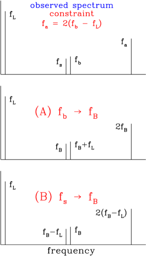
Figure 3.— Schematic Fourier amplitude spectrum. Note that $f_{s}={\frac{1}{2}}f_{a}$. Top diagram: Observed spectrum and frequency constraint. Middle and lower diagrams: Two possible sets of frequency assignments.

3. Discussion

We make the reasonable assumption, as in Mennickent, et al.  (2003), that one component is a tight binary of frequency $f_{B}$. We also assume that frequency $f_{L}$ is associated with a third object whose nature we leave unspecified at this stage. Note that the light curves, prewhitened with the frequency $f_{L}$ (which has the highest amplitude) and folded with $f_{a}$, either suggest or are compatible with eclipses or ellipsoidal variations. Two sets of frequency assignments are possible for $f_{b}$, Case A:

$$f_{s} \rightarrow f_{B}$$

$$f_{a} = 2f_{B}$$

$$f_{b} = f_{B}+f_{L}$$ (3)

or, Case B:

$$f_{b} \rightarrow f_{B}$$

$$f_{s} = f_{B}-f_{L}$$

$$f_{a} = 2(f_{B}-f_{L}).$$ (4)

These relations are displayed schematically in Fig. 3. We recall the observational conditions, namely (Table 1) that for all objects the Fourier amplitudes satisfy $A_{L}>A_{a}$, that both $A_{s}$ and $A_{b}$ are smaller than $A_{a}$, and that the ratio $A_{s}/A_{b}$ is close to unity, but can be above or below.

The combination frequency $f_{B}\pm f_{L}$ presumably is from radiation of the inner binary that is reprocessed (”reflected”) by the third object. Note that in case A the motion associated with frequency $f_{L}$ is retrograde, while in case B it is prograde.

In all of Table 1’s 11 objects, $f_{L}$ has the highest amplitude and appears to be reasonably sinusoidal (the harmonics have small amplitude). This means that most of the light variation is generated by a third object, separate from, but associated with the binary pair. Mennickent, et al.  (2003) suggest that the third object could be an orbiting disk or a precessing inclined disk. Other possibilities involve tides in a third star on an elliptical, long period orbit around the inner binary.

We prefer to separate the pure data analysis of these objects that has been presented in this paper from a discussion of the physical nature and modeling that we plan to address in a subsequent paper.

4. Summary

We have found a very clear relation of the form $f_{b}=f_{L}+f_{a}/2$ among the dominant observed Fourier frequencies $f_{L}$, $f_{b}$ and $f_{a}$ in 11 of the 30 LMC blue variables discussed in Mennickent, et al.  (2003). This relation is found in both MACHO bands, except for 2 objects where the $f_{b}$ peaks seem to be hidden in the noise in $M_{B}$. Accordingly, strong observational constraints apply to all 11 objects, namely (a) the frequency ratio $f_{b}/f_{L}\sim 35$ (or $f_{a}/f_{L}\sim 70$) found by Mennickent, et al.  (2003), (b) the linear 3-frequency relation of this paper, (c) the amplitude ratios of the 4 observed peaks (Table 1), and (d) the absence of other significant harmonics or peaks in the Fourier spectra. These conditions pose an interesting and serious challenge for development of a physical model for these 11 objects.

References

- Buchler, Wood & Soszynski (2009) Buchler, J.R., Wood, P.R. & Soszynski, I. 2009, ApJ, 698, 944
-
Kollath (2008)
Kollath, Z. 2008,
Occasional Technical Notes, No. 1, Konkoly Observatory,
see http://www.konkoly.hu/staff/kollath/mufran.html - Mennickent, et al. (2003) Mennickent, R. E., Pietrzynski, G., Diaz, M, & Gieren, W. 2003, A&A, 399, L47
- Press & Rybicki (1989) Press, W.H. & Rybicki, G.B. 1989, ApJ, 338, 277
- Stellingwerf (1978) Stellingwerf, R. F. 1978, ApJ, 224, 953
- D’Angelo, C. et al. (2006) D’Angelo, C., van Kerkwijk, M.H., & Rucinski, S.M. 2006, AJ, 132, 650
- Eggleton & Kiseleva-Eggleton (2001) Eggleton, P.P. & Kiseleva-Eggleton 2001, ApJ, 562, 1012
- Fabrycky & Tremaine (2007) Fabrycky, D. & Tremaine, S. 2007, ApJ, 669, 1298
- Kisleva et al. (1998) Kiseleva, L.G., Eggleton, P.P., & Mikkola, S. 1998, MNRAS, 300, 292
- Kozai (1962) Kozai, Y. 1962, AJ, 67, 591
- Mathis & Le Poncin-Lafitte (2009) Mathis, S. & Le Poncin-Lafitte, C. 2009, A&A, 497, 889
- Mazeh & Shaham (1979) Mazeh, T. & Shaham, J. 1979, A&A, 77, 145
- Pribulla & Rucinski (2006) Pribulla, T. & Rucinski, S.M., 2006, AJ, 131, 2986
- Tokovinin et al (2007) Tokovinin, A., Thomas, S., Sterzik, M., & Udry, S. 2006, A&A, 450, 681