Nonlinear power spectrum in the presence of massive neutrinos:
perturbation theory approach, galaxy bias and parameter forecasts

Abstract

Future or ongoing galaxy redshift surveys can put stringent constraints on neutrinos masses via the high-precision measurements of galaxy power spectrum, when combined with cosmic microwave background (CMB) information. In this paper we develop a method to model galaxy power spectrum in the weakly nonlinear regime for a mixed dark matter (CDM plus finite-mass neutrinos) model, based on perturbation theory (PT) whose validity is well tested by simulations for a CDM model. In doing this we carefully study various aspects of the nonlinear clustering (nonlinear neutrino perturbations and the higher-order growth functions), and then arrive at a useful approximation allowing for a quick computation of the nonlinear power spectrum as in the CDM case. The nonlinear galaxy bias is also included in a self-consistent manner within the PT framework. Thus the use of our PT model can give a more robust understanding of the measured galaxy power spectrum as well as allow for higher sensitivity to neutrino masses due to the gain of Fourier modes beyond the linear regime. Based on the Fisher matrix formalism, we find that BOSS or Stage-III type survey, when combined with Planck CMB information, gives a precision of total neutrino mass constraint, $\sigma(m_{\nu,{\rm tot}})\simeq 0.1$ eV, while Stage-IV type survey may achieve $\sigma(m_{\nu,{\rm tot}})\simeq 0.05~{}$eV, i.e. more than a $1$-$\sigma$ detection of neutrino masses. We also discuss possible systematic errors on dark energy parameters caused by the neutrino mass uncertainty. The significant correlation between neutrino mass and dark energy parameters is found, if the information on power spectrum amplitude is included. More importantly, for Stage-IV type survey, a best-fit dark energy model may be biased and falsely away from the underlying true model by more than the 1-$\sigma$ statistical errors, if neutrino mass is ignored in the model fitting.

I Introduction

The concordance $\Lambda$-dominated cold dark matter ($\Lambda$CDM) model for structure formation in the Universe is remarkably successful in describing various data sets such as cosmic microwave background (CMB) anisotropies, Type-Ia supernova distance measurements, observations of galaxy clustering and cluster counts, and weak gravitational lensing (e.g., Komatsu:2008aa ; Dodelson ). However, the concordance model requires that the present-day energy budget of the Universe is dominated by unknown two dark components. One is dark matter that is needed to explain the nonlinear aspects of gravitational clustering in structure formation, and the other is the cosmological constant contribution or perhaps a more generalized form dubbed as dark energy, which is needed to explain the cosmic accelerating expansion. Understanding the nature of these dark components is one of the most important, profound problems in cosmology as well as particle physics.

We now know that the Big-Bang relic neutrinos contribute to dark matter energy density by some small fraction, because the neutrino oscillation experiments exp1 ; exp2 ; exp3 ; exp4 have shown that neutrinos have finite masses (also see McKeown:2004yq ; Kayser:2005cd for a thorough review). However, the oscillation experiments are sensitive only to mass square differences between different flavor neutrinos, therefore the most fundamental constant of neutrinos, absolute mass scale, is not yet known, although the lower bound on total neutrino mass can be inferred as $m_{\nu,{\rm tot}}\raisebox{-2.15277pt}{$\>\stackrel{{\scriptstyle\textstyle>}}{{\sim}}\>$}0.06$ or $0.1$ eV for the normal and inverted mass hierarchies, respectively. On the other hand, the direct experiment has put only a weak upper bound on electron neutrino mass such as $m_{\nu_{e}}\raisebox{-2.15277pt}{$\>\stackrel{{\scriptstyle\textstyle<}}{{\sim}}\>$}2$ eV Bonn .

Cosmological probes can give a complementary, albeit indirect, method for constraining neutrino masses. There are two kinds of the methods. First is via the effect on cosmic expansion history. If neutrino species are massive enough as $m_{\nu}\raisebox{-2.15277pt}{$\>\stackrel{{\scriptstyle\textstyle>}}{{\sim}}\>$}0.5~{}$eV, the neutrinos became non-relativistic before recombination epoch and then imprint characteristic signatures onto structures of the CMB anisotropy spectra Ichikawa:2004zi ; Fukugita:2006rm . On the other hand, low-redshift geometrical probes such as Type-Ia supernovae (e.g. Kowalski ) and the Baryon Acoustic Oscillation (BAO) Eisenstein:2005su are sensitive to the present-day energy density of non-relativistic matter ($\Omega_{\rm m0}$) that is given by the sum of CDM, baryon and neutrino contributions: $\Omega_{\rm m0}\equiv\Omega_{\rm cdm0}+\Omega_{\rm b0}+\Omega_{\nu 0}$. Therefore combining these geometrical measurements can constrain neutrino mass: for example, Komatsu:2008aa already succeeded in obtaining the presumably best-available constraint from this method, $m_{\nu,{\rm tot}}\raisebox{-2.15277pt}{$\>\stackrel{{\scriptstyle\textstyle<}}{{\sim}}\>$}0.6~{}{\rm eV}$ (95% C.L.).

Alternative cosmological method is using clustering information of large-scale structure. Due to large velocities of the frozen Fermi-Dirac distribution, neutrinos cannot cluster on scales below the neutrino free-streaming scale that has a characteristic dependence on neutrino mass and redshift as given by $k_{{\rm fs},i}\simeq 0.023h{\rm Mpc}^{-1}(m_{\nu,i}/0.1{\rm eV})(\Omega_{m0}/0.23)[2/(1+z)]^{1/2}$, comparable with the BAO scales for neutrino mass scales of interest. As a result, the presence of finite-mass neutrinos suppresses the amplitude of low-redshift power spectrum on the small scales by at least the amount of a few percent, compared to the model without finite-mass neutrinos, for a fixed $\Omega_{\rm m0}$ Bond:1980 . Thus given the CMB normalization of primordial power spectrum, total neutrino mass can be explored by measuring clustering strengths of low-redshift large-scale structure via galaxy redshift survey Hu:1997mj ; Elgaroy:2002aa ; Tegmark:2006az , weak gravitational lensing Ichiki:2008ye ; Kitching:2008dp , Lyman-$\alpha$ forest power spectrum Seljak:2006bg and potentially 21cm observations Pritchard:2008wy . The existing data sets have put more stringent upper bounds on neutrino mass, $m_{\nu,{\rm tot}}\raisebox{-2.15277pt}{$\>\stackrel{{\scriptstyle\textstyle<}}{{\sim}}\>$}0.2$–$0.5$ eV, than the direct experiment limit, although some residual systematics are under discussion.

There are a number of ongoing and planned galaxy redshift surveys such as WiggleZ , FMOS Sumiyoshi:2009bf , BOSS , Subaru redshift survey known as the former project WFMOS , HETDEX , EUCLID , and JDEM . The primary scientific target of these surveys is exploring the nature of dark energy via the BAO experiment. At the same time these surveys promise to achieve the high-precision measurements of galaxy power spectrum amplitudes to a percent level precision at each wavenumber bins, and therefore offer a possibility to dramatically improve cosmological constraints including neutrino masses Takada:2005si ; Hannestad:2007cp ; Abdalla:2007ut .

Thus large-scale structure probes are very promising, however, the main obstacle is nonlinear effects such as nonlinear gravitational clustering, galaxy bias and redshift distortion. Recent theoretical studies have shown that, even at scales as large as $\sim 150h^{-1}$Mpc relevant for both the BAO and neutrino free-streaming scale, the standard linear theory, which gives remarkably successful agreement with CMB measurements, ceases to be accurate. The nonlinear effects are found to be significant compared to the precision of future surveys, using $N$-body simulations Jeong:2006xd ; Angulo:2007fw ; Takahashi:2008wn ; Sanchez:2008iw ; Seo:2008yx ; Jeong:2008rj ; Nishimichi:2008ry and analytical studies inspired from perturbation theory McDonald:2006hf ; Valageas:2006bi ; Matarrese:2007wc ; Nishimichi:2007xt ; Crocce:2007dt ; Matsubara:2007wj ; Taruya:2007xy ; Pietroni:2008jx ; Nomura:2008tm ; Carlson:2009it ; Taruya:2009ir . However in most of these studies the contribution of finite-mass neutrinos were ignored. The nonlinear effect of finite-mass neutrinos on the power spectrum needs to be understood in order to attain the full potential of future surveys, which is also important to minimize the possible systematic error on BAO experiments caused by the incorrect assumption that neutrinos are massless.

Therefore the aim of this paper is developing a formulation to model nonlinear galaxy power spectrum in a mixed dark matter (CDM plus finite-mass neutrinos) model, based on standard perturbation theory (SPT) (see Bernardeau:2001qr for a thorough review of perturbation theory for a CDM model). Here we mean by “standard” that the next-order corrections to the power spectrum, i.e. the one-loop corrections, are included. In doing this we carefully study various aspects of the nonlinear clustering: estimate the nonlinear neutrino perturbations by solving the collision-less Boltzmann equation hierarchies and study the higher-order growth functions of CDM plus baryon perturbations that have complicated scale- and redshift-dependences similarly to the linear-order growth rate. Then, given the detailed assessment of various effects, we will arrive at a useful approximation to compute the nonlinear matter power spectrum whose results were highlighted in Saito:2008bp . We then include a modeling of nonlinear galaxy bias self-consistently within the SPT framework following the method developed in McDonald:2006mx . Thus, while the nonlinear redshift distortion effect is not yet included, our model of the galaxy power spectrum can be compared to the actual measurement such as that in Tegmark:2006az , where the redshift distortion effect is removed using the Finger-of-God compression algorithm Tegmark:2004 . For preparation of such a study we will demonstrate parameter forecasts for neutrino mass constraints expected from some of galaxy surveys listed above, paying a particular attention on the correlation between neutrino mass and dark energy parameters in the weakly nonlinear regime. We also discuss a possible systematic error in the constraints on the dark energy parameter caused by the neutrino mass uncertainty.

The structure of this paper is as follows. In § II we develop the formulation of SPT method for computing the nonlinear matter power spectrum. In § III we then study the effect of finite-mass neutrinos on the matter power spectrum by varying the neutrino masses within the range inferred from the constraints. After including a model of nonlinear galaxy bias based on perturbation theory in § IV, we study parameter forecasts of neutrino masses and dark energy parameters using the Fisher matrix formalism in § V. § VI is devoted to summary and discussion. Unless explicitly stated, throughout this paper we assume the concordance $\Lambda$CDM-like cosmology with finite-mass neutrino contribution, which is consistent with the WMAP results Komatsu:2008aa . The fiducial model is: the density parameters are $\Omega_{\rm m0}=0.24,\ \Omega_{\rm m0}h^{2}=0.1277,$ and $\Omega_{\rm b0}h^{2}=0.0223$. The neutrino effect is studied by varying the neutrino mass scale. For simplicity the number of neutrino species is assumed to be $N_{\nu}=3$ because the matter power spectrum is sensitive to the sum of neutrino masses, $m_{\nu,{\rm tot}}=N_{\nu}m_{\nu}$. We assume a flat universe and consider $w_{0}=-1$ for dark energy equation of state. For the primordial fluctuation parameters, the amplitude, the tilt, and the running, are set to $\Delta^{2}_{\mathcal{R}}=2.35\times 10^{-9}$, $n_{\rm S}=1.0$, and $\alpha_{\rm S}=0$, respectively.

II Perturbation theory for nonlinear matter power spectrum in a MDM model

II.1 Preliminaries

First we write down basic equations to describe structure formation in a MDM model. Throughout this paper, we focus on the evolution of matter fluctuations consisting of MDM (CDM plus massive neutrinos) and baryon:

$$\delta_{\rm m}\equiv\frac{\delta\rho_{\rm c}+\delta\rho_{\rm b}+\delta\rho_{\nu}}{\rho_{\rm m}}=f_{\rm cb}\delta_{\rm cb}+f_{\nu}\delta_{\nu},$$ (1)

where the subscript ‘m’, ‘c’, ‘b’, ‘$\nu$’ and ‘cb’ stand for total matter, CDM, baryon, massive neutrinos, and CDM plus baryon, respectively, and $\delta_{\rm cb}$ and $\delta_{\nu}$ denote their density perturbations. The coefficients, $f_{\rm cb}$ and $f_{\nu}$, are the fractional contributions of each component to the present-day total matter density:

$$f_{\rm cb}=\frac{\Omega_{\rm c0}+\Omega_{\rm b0}}{\Omega_{\rm m0}},\quad f_{\nu}=\frac{\Omega_{\nu 0}}{\Omega_{\rm m0}}=1-f_{\rm cb}\simeq\frac{m_{\nu,{\rm tot}}}{94.1\Omega_{\rm m0}h^{2}},$$ (2)

with the density parameter, $\Omega_{i0}$, being defined as $\Omega_{i,0}\equiv 8\pi G\rho_{i}(t_{0})/(3H_{0}^{2})\ (i={\rm m,c,b,\nu})$ where the parameter, $h$, is dimensionless Hubble constant defined as $H_{0}=100h~{}{\rm kms^{-1}Mpc^{-1}}$. In the limit of $f_{\rm cb}\to 1$, the results shown below recover a CDM model which does not contain massive neutrinos. The evolution of homogeneous and isotropic universe is controlled by CDM, baryon, massive neutrinos and dark energy whose equation of state is simply assumed to be constant in time: $p_{\rm DE}=w_{0}\rho_{\rm DE}$ where $w_{0}$ is referred to as the equation of state parameter. Then, the background Friedman equations become

$$H^{2} = \frac{8\pi G}{3}\left(\rho_{\rm m}+\rho_{\rm DE}\right),$$ (3)

$$\dot{H} = -\frac{3}{2}\,H^{2}(1+w_{0}),$$ (4)

where the dot $\dot{\ }$ denotes the derivative with respect to cosmic time, $t$: $\dot{a}=da/dt$, and the Hubble parameter, $H$, is defined as $H\equiv\dot{a}/a$.

We are specifically concerned with the nonlinear growth of matter perturbations, $\delta_{\rm m}$. Let us first consider the contribution of CDM plus baryon perturbations, $\delta_{\rm cb}$, to the total matter perturbations. In order to evaluate the nonlinear evolution of $\delta_{\rm cb}$, we treat the CDM plus baryon components as a single pressure-less fluid. The continuity equation and the Euler equation for the CDM plus baryon fluctuations in Fourier space are given in Bernardeau:2001qr ; Taruya:1999vq as

$$H^{-1}\frac{\partial\delta_{\rm cb}(\mbox{\boldmath$k$};t)}{\partial t}+\theta_{\rm cb}(\mbox{\boldmath$k$};t)=\,-\int\frac{d^{3}\mbox{\boldmath$k$}^{\prime}}{(2\pi)^{3}}\,\alpha(\mbox{\boldmath$k$}^{\prime},\mbox{\boldmath$k$}-\mbox{\boldmath$k$}^{\prime})\,\delta_{\rm cb}(\mbox{\boldmath$k$}-\mbox{\boldmath$k$}^{\prime};t)\,\theta_{\rm cb}(\mbox{\boldmath$k$}^{\prime};t),$$ (5)

$$H^{-1}\frac{\partial\theta_{\rm cb}(\mbox{\boldmath$k$};t)}{\partial t}+\frac{1}{2}(1-3w_{0}\Omega_{\rm DE})\theta_{\rm cb}(\mbox{\boldmath$k$};t)+\frac{1}{2}(1-\Omega_{\rm DE})\delta_{\rm m}(\mbox{\boldmath$k$};t)$$

$$\quad\quad\quad\quad\quad\quad\quad\quad\quad~{}~{}~{}=\,-\frac{1}{2}\,\int\frac{d^{3}\mbox{\boldmath$k$}^{\prime}}{(2\pi)^{3}}\,\beta(\mbox{\boldmath$k$}^{\prime},\mbox{\boldmath$k$}-\mbox{\boldmath$k$}^{\prime})\,\theta_{\rm cb}(\mbox{\boldmath$k$}-\mbox{\boldmath$k$}^{\prime};t)\,\theta_{\rm cb}(\mbox{\boldmath$k$}^{\prime};t),$$ (6)

where the velocity divergence $\theta_{\rm cb}$ is defined as $\theta_{\rm cb}=\nabla\cdot\mbox{\boldmath$v$}_{\rm cb}/(aH)$ in real space. Note that we assume an irrotational flow, i.e. the vorticity is neglected Pueblas:2008uv . The Fourier kernels to describe the nonlinear mode coupling, $\alpha$ and $\beta$, are defined as

$$\alpha(\mbox{\boldmath$k$}_{1},\mbox{\boldmath$k$}_{2})\equiv 1+\frac{\mbox{\boldmath$k$}_{1}\cdot\mbox{\boldmath$k$}_{2}}{|\mbox{\boldmath$k$}_{1}|^{2}},\quad\quad\beta(\mbox{\boldmath$k$}_{1},\mbox{\boldmath$k$}_{2})\equiv\frac{(\mbox{\boldmath$k$}_{1}\cdot\mbox{\boldmath$k$}_{2})|\mbox{\boldmath$k$}_{1}+\mbox{\boldmath$k$}_{2}|^{2}}{|\mbox{\boldmath$k$}_{1}|^{2}|\mbox{\boldmath$k$}_{2}|^{2}}.$$ (7)

Taking the time-derivative of Eq.(5) and also using the Euler equation (6) yield the second-order differential equation for $\delta_{\rm cb}$:

$$\ddot{\delta_{\rm cb}}+2H\dot{\delta_{\rm cb}}-\frac{3}{2}H^{2}(1-\Omega_{\rm DE})\,\delta_{\rm m}$$

$$\quad\quad\quad=-\int\frac{d^{3}\mbox{\boldmath$k$}^{\prime}}{(2\pi)^{3}}\,\Bigl{[}\,\alpha(\mbox{\boldmath$k$}^{\prime},\mbox{\boldmath$k$}-\mbox{\boldmath$k$}^{\prime})\Bigl{\{}\,\left[H\,\delta_{\rm cb}(\mbox{\boldmath$k$}-\mbox{\boldmath$k$}^{\prime})\theta_{\rm cb}(\mbox{\boldmath$k$}^{\prime})\right]^{.}+2H^{2}\,\delta_{\rm cb}(\mbox{\boldmath$k$}-\mbox{\boldmath$k$}^{\prime})\theta_{\rm cb}(\mbox{\boldmath$k$}^{\prime})\,\Bigr{\}}\Bigr{.}$$

$$\quad\quad\quad\quad\quad\quad\quad\quad\quad\left.+\frac{1}{2}H^{2}\,\beta(\mbox{\boldmath$k$}^{\prime},\mbox{\boldmath$k$}-\mbox{\boldmath$k$}^{\prime})\,\theta_{\rm cb}(\mbox{\boldmath$k$}-\mbox{\boldmath$k$}^{\prime})\theta_{\rm cb}(\mbox{\boldmath$k$}^{\prime})\right].$$ (8)

Thus Eq. (8) contains $\delta_{\rm m}=f_{\rm cb}\delta_{\rm cb}+f_{\nu}\delta_{\nu}$ and cannot be solved unless the neutrino fluctuation field, $\delta_{\nu}$, is specified.

So let us move on to discussion on the neutrino perturbations. Unlike CDM and baryon, the finite-mass neutrinos have a large velocity dispersion following the frozen Fermi-Dirac distribution, and cannot be treated as fluids. Therefore, exactly speaking, it is necessary to solve Eq. (8) coupled with the collision-less Boltzmann equations for neutrino perturbations that include the nonlinear terms. This is still computationally expense, especially for solving the nonlinear Boltzmann equations. Here we rather consider the approximated method for solving the nonlinear perturbations as described in the next subsection, and will also assess an accuracy of the approximation.

In our method we focus on the linearized collision-less Boltzmann equations for neutrino perturbations Ma:1995ey :

$$\Psi^{\prime}_{0}=-\frac{qk}{a\epsilon}\Psi_{1}+H\phi\frac{d\ln f_{0}}{d\ln q},$$ (9)

$$\Psi^{\prime}_{1}=\frac{qk}{3a\epsilon}(\Psi_{0}-2\Psi_{2})-\frac{\epsilon k}{3aq}\phi\frac{d\ln f_{0}}{d\ln q},$$ (10)

$$\Psi^{\prime}_{\ell}=\frac{qk}{(2\ell+1)a\epsilon}[\ell\Psi_{\ell-1}-(\ell+1)\Psi_{\ell+1}]\ \ (\ell\geq 2),$$ (11)

where the variables, $q$ and $\epsilon$, are comoving 3-momentum and proper energy defined as $\epsilon\equiv(q^{2}+a^{2}m_{\nu,i}^{2})^{1/2}$, respectively, and the function $\phi$ is the gravitational potential perturbation under the conformal Newtonian gauge (see below). The superscript ’ denotes the derivative with respect to conformal time. The function $f_{0}$ is the zeroth-order (isotropic) Fermi-Dirac distribution, given as $f_{0}=2/(e^{\epsilon/aT}+1)$, and the function $\Psi$ is the linear-order perturbed distribution. The full phase-space distribution function of neutrinos is given in the linear regime as

$$f(x^{i},q_{j}/a,t)=f_{0}(q)[1+\Psi(x^{i},q,\hat{n}_{j},t)],$$ (12)

where the momentum vector is rewritten as $q_{j}=q\hat{n}_{j}$ with $\hat{n}_{j}\hat{n}^{j}=1$. The variables, $\Psi_{\ell}$, appearing in the Boltzmann equations above are the $\ell$-th moments in the Legendre expansion of $\Psi$:

$$\Psi(\mbox{\boldmath$k$},\hat{\bf n},q,t)=\sum^{\infty}_{\ell=0}(-i)^{\ell}(2\ell+1)\Psi_{\ell}(k,q,t)P_{\ell}(\hat{\mbox{\boldmath$k$}}\cdot\hat{\bf n}),$$ (13)

where $P_{\ell}$ is the $l$-th order Legendre polynomial. The neutrino density perturbation is given by integrating the monopole contribution of neutrino perturbations over momentum:

$$\delta_{\nu}(k,t)=\frac{4\pi}{a^{4}f_{\nu}\rho_{\rm m}}\int q^{2}dq\,\epsilon f_{0}(q)\Psi_{0}(k,q,t).$$ (14)

The system of momentum hierarchies, Eqs. (9), (10), and (11), can be solved once the gravitational potential $\phi$ is given. One of the Einstein equations, the Poisson equation, relates the potential $\phi$ to the total matter density perturbation $\delta_{\rm m}$ on subhorizon scales:

$$-k^{2}\phi(k,t)=4\pi Ga^{2}\rho_{\rm m}\delta_{\rm m}.$$ (15)

On scales smaller than the neutrinos’ free-streaming scale, $k\raisebox{-2.15277pt}{$\>\stackrel{{\scriptstyle\textstyle>}}{{\sim}}\>$}k_{\rm fs}$, the neutrino perturbation would be absent, and the Poisson equation roughly becomes $-k^{2}\phi(k,t)\approx 4\pi Ga^{2}\rho_{\rm m}f_{\rm cb}\delta_{\rm cb}$. Thus on these small scales the dynamics of neutrino perturbations are governed by the CDM plus baryon perturbations. We have so far written down all the basic equations that govern the dynamics of density perturbations for each components, $\delta_{\rm cb}$ and $\delta_{\nu}$. A quantity that is more relevant for actual large-scale structure probes such as galaxy clustering is the power spectrum of total matter including nonlinear corrections:

$$\langle\delta_{\rm m}(\mbox{\boldmath$k$};t)\delta_{\rm m}(\mbox{\boldmath$k$}^{\prime};t)\rangle=(2\pi)^{3}\delta_{D}(\mbox{\boldmath$k$}+\mbox{\boldmath$k$}^{\prime})P_{\rm m}(k;t).$$ (16)

The power spectrum, $P_{\rm m}$, is defined in terms of the density perturbations of CDM, baryon and neutrino perturbations as

$$P_{\rm m}(k;t)=f_{\rm cb}^{2}\,P_{\rm cb}(k;t)+2f_{\rm cb}f_{\nu}\,P_{\rm cb\nu}(k;t)+f_{\nu}^{2}\,P_{\nu}(k;t),$$ (17)

where $P_{\rm cb\nu}(k)$ is the cross spectrum between $\delta_{\rm cb}$ and $\delta_{\nu}$.

II.2 On the treatment of neutrino perturbation

Strictly speaking, in order to compute the total matter perturbation, $\delta_{\rm m}$, in the nonlinear regime, we need to solve Eq. (8) coupled with nonlinear collision-less Boltzmann equations for massive neutrinos, which seems computationally expensive. In order to avoid this obstacle, in this paper we employ a simple approximation that allows to analytically compute the nonlinear power spectrum in a MDM model based on the standard perturbation theory (SPT) (see Saito:2008bp for the similar discussion).

Let us begin with recalling characteristic properties of neutrino clustering on scales up to $k\sim 0.1~{}h{\rm Mpc}^{-1}$. Firstly, the neutrino perturbations contribute to nonlinear gravitational clustering via its contribution to the gravitational potential, where, implied in Eq. (15), the perturbation of physical neutrino density, $\delta\rho_{\nu}=\bar{\rho}_{\nu}\delta_{\nu}$, affects the gravitational potential. Thus the contribution is suppressed by a small factor $f_{\nu}$, currently limited as $f_{\nu}\raisebox{-2.15277pt}{$\>\stackrel{{\scriptstyle\textstyle<}}{{\sim}}\>$}0.05$ Komatsu:2008aa , even if the density perturbations of CDM and neutrinos are in similar amplitudes as predicted by the adiabatic structure formation scenario. Secondly, the neutrino perturbations would tend to stay in the linear regime due to the large velocity dispersion, at least on scales relevant for the BAO scales. These facts suggest that the nonlinear power spectrum arises mainly from the nonlinear perturbations of CDM plus baryon. Thus we model the nonlinear matter spectrum based on SPT (see below), but including only the linear-order perturbations of neutrinos:

$$P^{\rm NL}_{\rm m}(k;t)=f_{\rm cb}^{2}\,P^{\rm NL}_{\rm cb}(k;t)+2f_{\rm cb}f_{\nu}\,P^{\rm L}_{\rm cb\nu}(k;t)+f_{\nu}^{2}\,P^{\rm L}_{\nu}(k;t),$$ (18)

where the spectra with superscript “NL” denote the nonlinear spectra described below, and the spectra with “L” are the linear-order spectra. With this assumption, the neutrino perturbations can be precisely computed for given initial conditions by using the publicly available codes such as CMBFAST Seljak:1996 and CAMB Lewis:1999bs . The validity of our assumption is studied in detail in Appendix A. Here we briefly summarize the result. As explained around Eqs. (11) and (15), nonlinear clustering of neutrino perturbations is driven by nonlinear gravitational potential supported by CDM plus baryon perturbations, in a CDM dominated structure formation model. Therefore, the nonlinear correction to neutrino perturbations can be qualitatively estimated by solving the linearized Boltzmann equations (9)-(11), where the nonlinear gravitational potential due to the total matter density perturbations given by Eq. (18) is inserted into the gravitational force term (ignoring the nonlinear neutrino perturbations). The results are shown in Fig. 10. Nonlinear clustering indeed causes a nonlinear evolution of neutrino perturbations, deviating from the linear theory prediction. The nonlinear effect causes greater amplitudes of the neutrino perturbations on larger $k$ and at lower redshifts; e.g. the fractional difference between the linear and non-linear density perturbations $\delta_{\nu}^{\rm NL}/\delta^{\rm L}_{\nu}$ reaches to $\sim 10\%$ on $k\raisebox{-2.15277pt}{$\>\stackrel{{\scriptstyle\textstyle<}}{{\sim}}\>$}1~{}h$Mpc^-1 at $z=0$ for $f_{\nu}=0.05$. However, the nonlinear effect on the total matter power spectrum is suppressed by additional small factor $f_{\nu}$ as implied in Eq. (18). In conclusion the nonlinear correction to the total matter power spectrum is smaller than one percent level in the amplitude for a range of neutrino masses, $f_{\nu}\raisebox{-2.15277pt}{$\>\stackrel{{\scriptstyle\textstyle<}}{{\sim}}\>$}0.05$. For these reasons, throughout this paper, we employ the approximation (18), where the neutrinos affect nonlinear power spectrum of total matter via the effect on the growth rates of CDM plus baryon perturbations as described in the next section.

II.3 Perturbation Theory Approach

In this subsection we develop a method to compute nonlinear power spectrum of CDM plus baryon perturbations, $P_{\rm cb}(k;t)$ in a MDM model based on perturbation theory. First, in order to solve Eq. (8), we expand the density and velocity perturbations in a perturbative manner:

$$\delta_{\rm cb}=\delta_{\rm cb}^{(1)}+\delta_{\rm cb}^{(2)}+\delta_{\rm cb}^{(3)}+\cdots,\quad\quad\theta_{\rm cb}=\theta_{\rm cb}^{(1)}+\theta_{\rm cb}^{(2)}+\theta_{\rm cb}^{(3)}+\cdots,$$ (19)

where the superscript ‘($i$)’ denotes the $i$-th order perturbation. Here, we include the next-to-leading order corrections for $P_{\rm cb}(k;t)$, which are expressed as

$$P_{{\rm cb}}(k;t)=P^{{\rm L}}_{{\rm cb}}(k;t)+P^{(13)}_{{\rm cb}}(k;t)+P^{(22)}_{{\rm cb}}(k;t).$$ (20)

The first term $P^{{\rm L}}_{{\rm cb}}$ denotes the linear power spectrum of CDM plus baryon. The last two terms describe the nonlinear corrections, the so-called one-loop corrections, and the superscript ‘(13)’ and ‘(22)’ denote the multiplied order of perturbations, $\langle\delta_{\rm cb}^{(1)}\delta_{\rm cb}^{(3)}\rangle$ and $\langle\delta_{\rm cb}^{(2)}\delta_{\rm cb}^{(2)}\rangle$. We thus include contributions up to the third-order perturbations.

Inserting the formal solutions (19) into Eq. (8) gives, at the lowest order of perturbations, the differential equation for $\delta_{\rm cb}^{{(1)}}$:

$$\ddot{\delta_{\rm cb}}^{(1)}+2H\dot{\delta_{\rm cb}}^{(1)}-\frac{3}{2}H^{2}(1-\Omega_{\rm DE})\,\delta_{\rm m}^{(1)}=0.$$ (21)

This equation can be straightforwardly solved, together with the linearized Boltzmann equation for neutrino perturbations (e.g., Lesgourgues:2006nd ). In this paper we use CAMB Lewis:1999bs to obtain the accurate solution of $\delta_{\rm cb}^{{(1)}}$. Before moving on to the higher-order perturbations of $\delta_{\rm cb}$, for convenience of our discussion, we formally write down the linear-order solutions of density and velocity perturbations expressed as Eisenstein:1997jh ; Hu:1997vi :

$$\delta_{\rm cb}^{(1)}(\mbox{\boldmath$k$};t)=D_{\rm cb}(k;t)\,\hat{\Delta}(\mbox{\boldmath$k$}),\quad\quad\theta_{\rm cb}^{(1)}(\mbox{\boldmath$k$};t)=-\frac{dD_{\rm cb}(k;t)}{d\ln a}\,\hat{\Delta}(\mbox{\boldmath$k$}),$$ (22)

where the quantity $\hat{\Delta}(\mbox{\boldmath$k$})$ represents the initial perturbation variables at an early epoch $t_{\rm ini}$, sufficiently in the linear regime, e.g. the Compton-drag epoch. The ensemble average gives the initial power spectrum:

$$\langle\hat{\Delta}(\mbox{\boldmath$k$})\hat{\Delta}(\mbox{\boldmath$k$}^{\prime})\rangle=(2\pi)^{3}\delta_{D}(\mbox{\boldmath$k$}+\mbox{\boldmath$k$}^{\prime})\,\,P^{\rm L}_{\rm cb}(k;t_{\rm ini}).$$ (23)

The effect of massive neutrinos can thus be described as the scale-dependent growth function, $D_{\rm cb}(k;t)$. At wavenumbers smaller than the neutrino free-streaming scale, $k_{\rm fs}$, the neutrinos can cluster together with CDM and baryon. On the other hand, at $k>k_{\rm fs}$, the growth of CDM plus baryon perturbations is suppressed due to the weaker gravitational force caused by the lack of neutrino perturbations. Thus the growth function has asymptotic behaviors given in Lesgourgues:2006nd as

$$D_{\rm cb}(k;t)\propto\left\{\begin{array}[]{cc}D_{1}(t)&(k\ll k_{\rm fs})\\ D_{1}(t)^{1-p}&(k\gg k_{\rm fs})\end{array}\right.,$$ (24)

where $D_{1}(z)$ is the growth rate for a CDM model without massive neutrinos, but with the same matter density $\Omega_{\rm m0}$ to that of the MDM model (in this case the growth rate has no scale dependence), and the parameter $p$ is defined as $p\equiv(5-\sqrt{25-24f_{\nu}})/4$.

We now consider the second- and third-order perturbations. Substituting the linear solutions into the r.h.s of Eq. (8) yields the differential equation for the second-order perturbation $\delta_{\rm cb}^{(2)}$:

$$\ddot{\delta_{\rm cb}}^{(2)}+2H\dot{\delta_{\rm cb}}^{(2)}-\frac{3}{2}H^{2}(1-\Omega_{\rm DE})\,f_{\rm cb}\delta_{\rm cb}^{(2)}=\int\frac{d^{3}\mbox{\boldmath$k$}_{1}d^{3}\mbox{\boldmath$k$}_{2}}{(2\pi)^{3}}\,\,\delta_{D}(\mbox{\boldmath$k$}-\mbox{\boldmath$k$}_{1}-\mbox{\boldmath$k$}_{2})\hat{\Delta}(\mbox{\boldmath$k$}_{1})\hat{\Delta}(\mbox{\boldmath$k$}_{2})$$

$$\quad\quad\quad\quad\times\,\,\Bigl{[}\,\alpha(\mbox{\boldmath$k$}_{1},\mbox{\boldmath$k$}_{2})\Bigl{\{}\,\left[H\,\frac{dD_{\rm cb}(k_{1})}{d\ln a}D_{\rm cb}(k_{2})\right]^{.}+2H^{2}\,\frac{dD_{\rm cb}(k_{1})}{d\ln a}D_{\rm cb}(k_{2})\,\Bigr{\}}$$

$$\quad\quad\quad\quad\quad\quad\quad\quad\quad\quad\quad\quad\quad\quad\quad\quad\quad+\,\beta(\mbox{\boldmath$k$}_{1},\mbox{\boldmath$k$}_{2})\,\,\frac{1}{2}H^{2}\,\frac{dD_{\rm cb}(k_{1})}{d\ln a}\frac{dD_{\rm cb}(k_{2})}{d\ln a}\,\Bigr{]},$$ (25)

where, as described in the preceding section, we have ignored the second-order contribution of neutrino perturbations, i.e. set $\delta_{\nu}^{(2)}=0$, and therefore used $\delta_{\rm m}^{(2)}=f_{\rm cb}\delta_{\rm cb}^{(2)}$ in deriving the equation above. The formal solutions of Eq. (25) can be written as

$$\delta_{\rm cb}^{(2)}(\mbox{\boldmath$k$};t) = \int\frac{d^{3}\mbox{\boldmath$k$}_{1}d^{3}\mbox{\boldmath$k$}_{2}}{(2\pi)^{3}}\,\,\delta_{D}(\mbox{\boldmath$k$}-\mbox{\boldmath$k$}_{1}-\mbox{\boldmath$k$}_{2})\hat{\Delta}(\mbox{\boldmath$k$}_{1})\hat{\Delta}(\mbox{\boldmath$k$}_{2})$$ (26)

$$\quad\quad\quad\quad\quad\quad\times\,\Bigl{[}\,\alpha(\mbox{\boldmath$k$}_{1},\mbox{\boldmath$k$}_{2})A^{(2)}_{\delta}(k_{1},k_{2};t)+\,\beta(\mbox{\boldmath$k$}_{1},\mbox{\boldmath$k$}_{2})B^{(2)}_{\delta}(k_{1},k_{2};t)\Bigr{]},$$

where $A^{(2)}_{\delta}$ and $B^{(2)}_{\delta}$ are the second-order growth functions given in detail in Appendix  B

There are notable differences between the second-order perturbations in models with and without massive neutrinos. Firstly, the second-order growth functions $A^{(2)}_{\delta}$ and $B^{(2)}_{\delta}$ are scale-dependent originating from the scale-dependence of the linear growth rate. Thus additional nonlinear mode coupling arises via the scale-dependent growth rate, in addition to via the shape of the input linear power spectrum. Secondly, the gravitational force is weaker in a MDM model because we ignored the second-order neutrino perturbations in our method, i.e., $\delta_{\rm m}^{(2)}=f_{\rm cb}\delta_{\rm cb}^{(2)}$ with $f_{\rm cb}<1$. These imply that the second-order density perturbations are suppressed compare to those of CDM model with same $\Omega_{\rm m0}$. We will in detail show the results below.

Similarly, a formal solution of the third-order perturbation can be expressed as

$$\delta_{\rm cb}^{(3)}(\mbox{\boldmath$k$};t) = \int\frac{d^{3}\mbox{\boldmath$k$}_{1}d^{3}\mbox{\boldmath$k$}_{2}d^{3}\mbox{\boldmath$k$}_{3}}{(2\pi)^{6}}\,\delta_{D}(\mbox{\boldmath$k$}-\mbox{\boldmath$k$}_{1}-\mbox{\boldmath$k$}_{2}-\mbox{\boldmath$k$}_{3})\hat{\Delta}(\mbox{\boldmath$k$}_{1})\hat{\Delta}(\mbox{\boldmath$k$}_{2})\hat{\Delta}(\mbox{\boldmath$k$}_{3})$$ (27)

$$\times\,\left[\,\alpha_{1,23}\{\alpha_{2,3}A^{(3)}_{\delta 1,2,3}(t)+\beta_{2,3}B^{(3)}_{\delta 1,2,3}(t)\}-\alpha_{23,1}\{\alpha_{2,3}C^{(3)}_{\delta 1,2,3}(t)+\beta_{2,3}D^{(3)}_{\delta 1,2,3}(t)\}\right.$$

$$\quad\quad\quad-\beta_{1,23}\{\alpha_{2,3}E^{(3)}_{\delta 1,2,3}(t)+\beta_{2,3}F^{(3)}_{\delta 1,2,3}(t)\},$$

where the Fourier kernels $\alpha(\mbox{\boldmath$k$}_{1},\mbox{\boldmath$k$}_{2})$, $\beta(\mbox{\boldmath$k$}_{1},\mbox{\boldmath$k$}_{2})$ and $\alpha(\mbox{\boldmath$k$}_{1},\mbox{\boldmath$k$}_{2}+\mbox{\boldmath$k$}_{3})$ are abbreviated as $\alpha_{1,2}$, $\beta_{1,2}$ and $\alpha_{1,23}$ respectively, and the third-order growth functions $\mathcal{I}^{(3)}_{\delta}\,(\mathcal{I}=A,B,C,D,E,F)$, abbreviated as $\mathcal{I}^{(3)}_{\delta}(k_{1},k_{2},k_{3})=\mathcal{I}^{(3)}_{\delta 1,2,3}$ and so on, are given in Appendix B.

II.4 One-loop Corrections to $P_{\rm cb}$

We now study the higher-order density perturbations for a given MDM model. Using the formal solutions, we can derive the explicit expressions for the one-loop corrections to $P_{\rm cb}$. First let us consider $P^{(22)}_{\rm cb}$. Using Eq. (26), the ensemble average $\langle\delta_{\rm cb}^{(2)}(\mbox{\boldmath$k$};t)\delta_{\rm cb}^{(2)}(\mbox{\boldmath$k$}^{\prime};t)\rangle$ yields the power spectrum $P_{\rm cb}^{(22)}$:

$$P^{(22)}_{\rm cb}(k;t)=2\int\left.\frac{d^{3}\mbox{\boldmath$k$}_{1}}{(2\pi)^{3}}[\alpha_{1,2}A^{(2)}_{\delta 1,2}(t)+\beta_{1,2}B^{(2)}_{\delta 1,2}(t)]^{2}P^{\rm L}_{\rm cb}(k_{1},t_{\rm ini})P^{\rm L}_{\rm cb}(k_{2},t_{\rm ini})\right|_{\mbox{\boldmath$k$}=\mbox{\boldmath$k$}_{1}+\mbox{\boldmath$k$}_{2}},$$ (28)

where we have used the abbreviated expressions such as $A^{(2)}_{\delta}(k_{1},k_{2},t)=A^{(2)}_{\delta,1,2}(t)$, and the $\mbox{\boldmath$k$}_{1}$-integration has to be done under the condition $\mbox{\boldmath$k$}=\mbox{\boldmath$k$}_{1}+\mbox{\boldmath$k$}_{2}$. The prefactor 2 arises from the Wick’s theorem in evaluating the ensemble average, $\langle\Delta(\mbox{\boldmath$k$}_{1})\Delta(\mbox{\boldmath$k$}_{2})\Delta(\mbox{\boldmath$k$}_{3})\Delta(\mbox{\boldmath$k$}_{4})\rangle$. Changing the integration variables to $\mbox{\boldmath$r$}\equiv\mbox{\boldmath$k$}_{1}/k$ and $\mu\equiv\mbox{\boldmath$k$}\cdot\mbox{\boldmath$k$}_{1}/(k\,k_{1})$, the expression of $P^{(22)}_{\rm cb}$ is rewritten as

$$P_{\rm cb,\,MDM}^{(22)}(k;t) = \frac{k^{3}}{2\pi^{2}}\int^{\infty}_{0}r^{2}drP^{\rm L}_{\rm cb}(kr;t)\int^{1}_{-1}d\mu\,P^{\rm L}_{\rm cb}(k\sqrt{1+r^{2}-2r\mu};t)\mathcal{K}^{(2)}_{\delta}(k,r,\mu;t),$$ (29)

where $P^{\rm L}(k;t)$ is the linear spectrum at time $t$, given in terms of the initial spectrum as $P^{\rm L}(k;t)\equiv D_{1}(t)^{2}P^{\rm L}(k;t_{i})$, and $\mathcal{K}$ is the function containing the growth functions, which is defined as

$$\mathcal{K}^{(2)}_{\delta}(k,r,\mu;t) = \left[\frac{1}{2}\left(\frac{\mu}{r}\frac{A^{(2)}_{\delta 1,2}(t)}{D_{\rm cb}(kr;t)D_{\rm cb}(k\sqrt{1+r^{2}-2r\mu};t)}\right.\right.$$ (30)

$$\quad\quad+\left.\frac{1-r\mu}{1+r^{2}-2r\mu}\frac{A^{(2)}_{\delta 2,1}(t)}{D_{\rm cb}(kr;t)D_{\rm cb}(k\sqrt{1+r^{2}-2r\mu};t)}\right)$$

$$\quad\left.+\frac{\mu-r}{r(1+r^{2}-2r\mu)}\frac{B^{(2)}_{\delta 1,2}(t)}{D_{\rm cb}(kr;t)D_{\rm cb}(k\sqrt{1+r^{2}-2r\mu};t)}\right]^{2}.$$

For the CDM model case (the case without massive neutrinos), i.e. the limit $f_{\rm cb}\to 1$, the higher-order growth functions become scale-independent as a result of the scale-independence of the linear growth rate. In this case, the growth functions are well approximated as

$$\frac{A^{(2)}_{\delta 1,2}(t)}{D_{\rm cb}(kr;t)D_{\rm cb}(k\sqrt{1+r^{2}-2r\mu};t)}\to\frac{5}{7},$$

$$\frac{B^{(2)}_{\delta 1,2}(t)}{D_{\rm cb}(kr;t)D_{\rm cb}(k\sqrt{1+r^{2}-2r\mu};t)}\to\frac{1}{7}.$$ (31)

Note that the asymptotic behaviors above are exact only in an Einstein de-Sitter model ($\Omega_{\rm m0}=1$), but hold an excellent approximation for a CDM model at relevant redshifts Bernardeau:1993qu ; Takahashi:2008yk . Hence, for the case $f_{\rm cb}=1$, Eq. (29) recovers a well-known expression of the one-loop power spectrum $P^{(22)}_{\rm CDM}(k,t)$ for the CDM model case Makino:1992a ; Jain:1994a :

$$P^{(22)}_{\rm cb}~{}\to~{}P^{(22)}_{\rm cb}(k;t)=\frac{k^{3}}{98(2\pi)^{2}}\int^{\infty}_{0}dr\,P^{\rm L}_{\rm cb}(kr;t)$$

$$\quad\quad\quad\quad\quad\quad\times\int^{1}_{-1}d\mu\,P^{L}_{\rm cb}(k\sqrt{1+r^{2}-2r\mu};t)\frac{(3r+7\mu-10r\mu^{2})^{2}}{(1+r^{2}-2r\mu)^{2}}.$$ (32)

Thus, for a MDM model, the scale-dependent growth function (Eq. [30]) has to be solved before obtaining the the power spectrum $P^{(22)}_{\rm cb}$. Because of this, the exact computation of $P_{\rm cb}^{(22)}$ is computationally expensive.

Similarly, another one-loop power spectrum, $P^{(13)}_{\rm cb}$, is formally expressed as

$$P^{(13)}_{\rm cb,\,MDM}(k;t) = \frac{2k^{3}P^{\rm L}_{\rm cb}(k;t)}{(2\pi)^{2}}\int^{\infty}_{0}dr\;r^{2}P_{\rm cb}^{\rm L}(kr;t)\mathcal{K}^{(3)}_{\delta}(k,r;t),$$ (33)

where the growth function $\mathcal{K}^{(3)}_{\delta}$ is defined as

$$\mathcal{K}^{(3)}_{\delta}(k,r;t) = \frac{1}{D_{\rm cb}(k;t)D_{\rm cb}(kr;t)^{2}}\left[-\frac{2}{3}\left\{A^{(3)}_{\delta}(kr,k,kr;t)+\frac{1}{r^{2}}A^{(3)}_{\delta}(kr,kr,k;t)\right\}\right.$$ (34)

$$\quad\quad-\frac{2(1+r^{2})}{3r^{2}}\left\{B^{(3)}_{\delta}(kr,k,kr;t)+B^{(3)}_{\delta}(kr,kr,k;t)\right\}$$

$$\quad\quad+\left\{\frac{-3+r^{2}}{2}-\frac{(1-r^{2})^{2}}{4r}\ln\left|\frac{1+r}{1-r}\right|\right\}C^{(3)}_{\delta}(kr,k,kr;t)$$

$$\quad\quad+\left\{\frac{-1-r^{2}}{2r^{2}}+\frac{(1-r^{2})^{2}}{4r^{3}}\ln\left|\frac{1+r}{1-r}\right|\right\}C^{(3)}_{\delta}(kr,kr,k;t)$$

$$\quad\quad-\frac{2}{3}\left\{D^{(3)}_{\delta}(kr,k,kr;t)+D^{(3)}_{\delta}(kr,kr,k;t)\right\}$$

$$\quad\quad+\left\{\frac{1+r^{2}}{2r^{2}}-\frac{(1-r^{2})^{2}}{4r^{3}}\ln\left|\frac{1+r}{1-r}\right|\right\}E^{(3)}_{\delta}(kr,k,kr;t)$$

$$\quad\quad+\left\{\frac{-1+3r^{2}}{2r^{4}}+\frac{(1-r^{2})^{2}}{4r^{5}}\ln\left|\frac{1+r}{1-r}\right|\right\}E^{(3)}_{\delta}(kr,kr,k;t)$$

$$\quad\quad\left.+\frac{2}{3r^{2}}\left\{F^{(3)}_{\delta}(kr,k,kr;t)+F^{(3)}_{\delta}(kr,kr,k;t)\right\}\right].$$

Note that $P^{(13)}_{\rm cb}$ is evaluated by one-dimensional integration once the linear power spectrum and the growth function are given. For a model without massive neutrinos, the growth functions are approximated as

$$\frac{1}{D_{\rm cb}(k;t)D_{\rm cb}(kr;t)^{2}}\left\{A_{\delta}^{(3)},B_{\delta}^{(3)},C_{\delta}^{(3)},D_{\delta}^{(3)},E_{\delta}^{(3)},F_{\delta}^{(3)}\right\}\to\left\{\frac{5}{18},\frac{1}{18},-\frac{1}{6},-\frac{1}{9},-\frac{1}{21},-\frac{2}{63}\right\}.$$ (35)

Therefore, Eq. (33) recovers the expression of $P^{{(13)}}$ for the CDM model case:

$$P^{(13)}_{\rm cb}~{}\to~{}P^{(13)}_{\rm cb}(k;t)=\frac{k^{3}}{252(2\pi)^{2}}P^{\rm L}_{\rm cb}(k;t)\int^{\infty}_{0}drP^{\rm L}_{\rm cb}(k;t)$$

$$\quad\quad\quad\quad\quad\quad\times\left[\frac{12}{r^{2}}-158+100r^{2}-42r^{4}+\frac{3}{r^{3}}(r^{2}-1)^{3}(7r^{2}+2)\ln\left|\frac{1+r}{1-r}\right|\right].$$ (36)

Again, an exact computation of $P^{(13)}_{\rm cb}$ is computationally expensive.

Thus evaluations of the one-loop correction spectra, $P^{(12)}_{\rm cb}$ and $P^{(13)}_{\rm cb}$, at each $k$ and each time $t$ require high-dimension integrations, which are numerically time-consuming. Rather, we find that Eqs. (32) and (36) serve as a good approximations to obtain the spectra for a MDM model, if the scale-dependent linear growth rate entering into the linear power spectrum $P^{\rm L}_{\rm cb}$ is properly taken into account. We below give the justification.

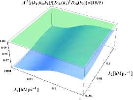
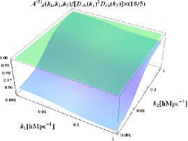
First, we study validity of the approximations (31) and (35) for the nonlinear growth functions in a MDM model. Fig. 1 compares the approximations  (31) and (35) with the results obtained by numerically solving the differential equations (50), (51) and (53) that govern time-evolution of the nonlinear growth functions . Here we consider the growth functions $A_{\delta}^{(2)}(k_{1},k_{2})$ and $A_{\delta}^{(3)}(k_{1},k_{2},k_{3})$ as representative examples. Also note that we considered $f_{\nu}=0.05$, corresponding to the current upper bound, and redshift $z=0$, where nonlinear clustering is strongly evolved. This figure clearly shows that the fractional errors of the approximations are less than $\sim 5\%$ over a wide range of wavenumbers we have considered. This agreement implies that the scale-dependence of higher-order growth functions are well-captured by the $k$-dependence of linear growth rate, $D_{\rm cb}(k;t)$. This level agreement was also found for other growth functions, $B_{\delta}^{(3)}$, $C_{\delta}^{(3)}$, $D_{\delta}^{(3)}$, $E_{\delta}^{(3)}$, and $F_{\delta}^{(3)}$.

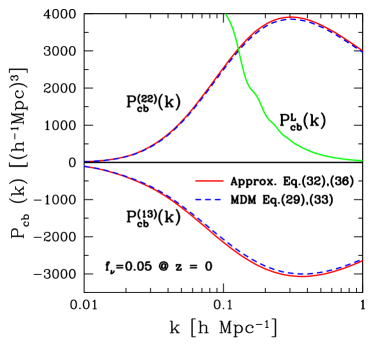
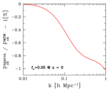
Fig. 2 compares the approximation with the full evaluation of one-loop power spectra, $P^{(22)}_{\rm cb}(k)$ and $P^{(13)}_{\rm cb}(k)$. In the left panel, the dashed curves show the result obtained by performing the numerical integrations in Eqs. (29) and (33) where the high-order growth functions are inserted into the calculations of the Fourier kernels $\mathcal{K}^{(2)}_{\delta}$ and $\mathcal{K}^{(3)}_{\delta}$, while the solid curves are the results obtained by the approximations (32) and (36). Note that we assumed $f_{\nu}=0.05$ as in Fig. 1. It is apparent that the absolute values of $P^{(22)}_{\rm cb}(k)$ and $P^{(13)}_{\rm cb}(k)$ are slightly overestimated by the approximations, because the higher-order growth functions are overestimated by the approximations as implied in Fig. 1. The right panel shows the resulting total power spectra of baryon plus CDM perturbations that include up to the one-loop corrections: $P_{\rm cb}=P_{\rm cb}^{\rm L}+P_{\rm cb}^{(22)}+P_{\rm cb}^{(13)}$. It is found that the fractional error of the approximation is smaller than $\sim 1\%$ on scales up to $k=1h$Mpc^-1, for the case of $f_{\nu}=0.05$. Thus we can conclude that the approximations to compute the one-loop power spectra are sufficiently accurate for our purpose, over ranges of wavenumbers, redshifts and neutrino mass scales we are interested in.

Given the results shown in Figs. 1 and 2, we will hereafter employ the approximations (32) and (36) for computing the nonlinear power spectrum of total matter at an arbitrary time $t$. A brief summary is: we first compute the linear power spectra of each components at time $t$, $P^{\rm L}_{\rm cb}(k;t)$, $P_{\rm\nu}^{\rm L}(k;t)$, and $P^{\rm L}_{\rm cb\nu}(k;t)$, for a desired MDM model, by using the publicly available code CAMB Lewis:1999bs . We then compute one-loop power spectra, $P^{(22)}_{\rm cb}(k;t)$ and $P^{(13)}_{\rm cb}(k;t)$, using Eqs. (32) and (36). Then, all the spectra are summed up to obtain the nonlinear spectrum of total matter:

$$P^{\rm NL}_{\rm m}(k;z)=f_{\rm cb}^{2}[P^{L}_{\rm cb}(k;z)+P^{(22)}_{\rm cb}(k;z)+P^{(13)}_{\rm cb}(k;z)]+2f_{\rm cb}f_{\nu}P^{L}_{\rm cb\nu}(k;z)+f_{\nu}^{2}P^{L}_{\nu}(k;z).$$ (37)

Before closing this sub-section, we comment on the work of Wong:2008ws , where a similar method for computing the one-loop corrected power spectra for a MDM model was developed based on perturbation theory ignoring the nonlinear neutrino perturbations. Although our method is qualitatively equivalent to their method, there are several technical differences that may be worth stressing. Wong:2008ws first employed the analytical fitting formula for scale-dependent linear growth function (also for the transfer function) developed in Eisenstein:1997jh , which is given as a function of neutrino masses and cosmological parameters. Then, analytical expressions for the higher-order growth functions and the one-loop power spectra were derived. There are several inaccuracies involved in the fitting formula. The formula becomes less accurate for small neutrino masses as explicitly pointed out in Kiakotou:2007pz . More precisely for a case that neutrino(s) is massive enough such that the neutrinos become non-relativistic in the radiation dominated era, corresponding to $m_{\nu}\raisebox{-2.15277pt}{$\>\stackrel{{\scriptstyle\textstyle>}}{{\sim}}\>$}0.6~{}{\rm eV}$ ($f_{\nu}\raisebox{-2.15277pt}{$\>\stackrel{{\scriptstyle\textstyle>}}{{\sim}}\>$}0.05$) for a $\Lambda$CDM model, the fitting formula becomes inaccurate because it assumes a continuous suppression in the matter growth since neutrinos became the non-relativistic, although the suppression occurs only in the matter dominated regime. In addition the fitting formula does not include BAO features in the transfer function. Therefore, the use of the fitting formula may under-estimate the ability of future galaxy surveys for constraining cosmological parameters, especially dark energy parameters to which the observed scales of BAO peaks are sensitive. In contrast, in our method, the nonlinear power spectrum is obtained by inserting the linear power spectrum outputs of the numerical Boltzmann solver such as CAMB, which takes into account the scale-dependent growth rate as well as BAO features at high precision. Albeit these small differences, Wong:2008ws also verified that Eqs. (32) and (36) are good approximation.

Figure 1: The 2nd- and 3rd-order growth functions at redshift $z=0$ are plotted as a function of two wavenumbers $k_{1}$ and $k_{2}$, for a MDM model with $f_{\nu}=0.05$ ($m_{\nu,{\rm tot}}\simeq 0.6~{}$eV). As representative examples, shown here is the growth functions divided by some powers of the linear growth rate: $A^{(2)}_{\delta}(k_{1},k_{2})/[D_{\rm cb}(k_{1})D_{\rm cb}(k_{2})(5/7)]$ (left panel), $A^{(3)}_{\delta}(k_{1},k_{2},k_{1})/[D_{\rm cb}(k_{1})^{2}D_{\rm cb}(k_{2})(5/18)]$ (middle) and $A^{(3)}_{\delta}(k_{1},k_{1},k_{2})/[D_{\rm cb}(k_{1})^{2}D_{\rm cb}(k_{2})(5/18)]$ (right), respectively. Note that specific combinations of $k_{i}$-arguments in $A^{(3)}_{\delta}$ are chosen because the one-loop power spectrum $P_{\rm cb}^{(13)}$ (see Eq. [33]) depends on the growth functions of specific configurations. The quantities shown become unity for the limit $f_{\nu}=0$, i.e. a model without massive neutrinos (see Eqs. [31] and [35]), which is shown by the plane in each plot. Therefore the deviations from unity reflect additional scale dependences arising from the mode-coupling. It is clear that scale-dependences of the higher-order growth functions are well-captured by combinations of the linear growth rate, and the approximations (31) and (35) hold valid with accuracy better than $\sim 5\%$ over a range of wavenumbers we have considered.

Figure 2: Left panel: The dashed curves show the one-loop power spectra of CDM plus baryon perturbations, $P^{(22)}_{\rm cb}$ and $P^{(13)}_{\rm cb}$, which are obtained by numerical integrations of Eqs. (29) and (33), respectively, while the solid curves show the spectra computed using the approximations (32) and (36). Note that the $y$-axis is plotted in the linear scale, and we consider $f_{\nu}=0.05$ and $z=0$. For comparison, the rightmost solid curve labelled as “$P_{\rm cb}^{\rm L}$” shows the linear power spectrum. Right panel: The fractional difference of the total matter power spectrum including up to the one-loop corrections is shown in the left panel: $P^{\rm NL}_{\rm cb}(k)=P^{\rm L}_{\rm cb}(k)+P^{(13)}_{\rm cb}(k)+P^{(22)}_{\rm cb}(k)$. The approximation is found to be accurate to better than $1\%$ on scales $k\raisebox{-2.15277pt}{$\>\stackrel{{\scriptstyle\textstyle<}}{{\sim}}\>$}1h$Mpc^-1.

III Nonlinear power spectrum in a MDM model

In this section, based on the treatment developed in the previous section, we study effects of finite mass neutrinos on the nonlinear power spectrum of total matter.

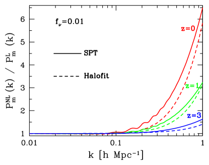
In Fig. 3 we show the SPT predictions for nonlinear power spectra divided by the linear power spectra at three different redshifts $z=0$, 1 and $3$, respectively, for a MDM model with $f_{\nu}=0.01$ ($m_{\nu,{\rm tot}}\simeq 0.12~{}$eV). Nonlinear gravitational clustering causes amplitudes of the nonlinear total matter power spectrum to be enhanced, resulting in more significant deviations from the linear theory predictions on smaller scales and at lower redshifts. In other words our PT model tells the range of wavenumbers and redshifts where the linear theory is valid or equivalently the linear theory starts to break down on wavenumbers beyond the applicable range. Our model predictions are also compared with the result of an empirical method, which is the halo model approach (hereafter we call ‘halofit’). In this model the nonlinear power spectrum is obtained by mapping the input linear power spectrum based on the fitting formula that is calibrated by numerical simulations for CDM models Smith:2002dz . Recent studies Ichiki:2008ye employed the halofit method to compare the model predictions to the weak lensing measurements for a MDM model, and then derived an upper limit on total neutrino mass as $m_{\nu,{\rm tot}}\raisebox{-2.15277pt}{$\>\stackrel{{\scriptstyle\textstyle<}}{{\sim}}\>$}0.54~{}{\rm eV}$ (95%C.L.). The halofit power spectra are smaller in amplitudes than SPT by up to $\sim 10\%$ over a range of scales we consider. Furthermore, SPT more washes out oscillatory BAO features than halofit, as pointed out in the previous study Jeong:2006xd , where the SPT results were shown to better reproduce the simulations results than the halofit results.

It should also be noted that SPT eventually ceases to be accurate at smaller scales, and the validity needs to be carefully studied by using numerical simulations (e.g., Nishimichi:2008ry for such a study for a CDM model). Our method may be further improved by including the higher-order perturbation contributions or using a refined method such as the renormalized perturbation theory (e.g. Crocce:2007dt ) or the closure theory method Taruya:2007xy . These are in progress and will be presented elsewhere.

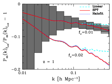
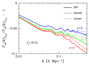
In the left panel of Fig. 4 we compare the two power spectra with and without massive neutrinos, $P_{f_{\nu}\neq 0}/P_{f_{\nu}=0}$, for a fixed $\Omega_{\rm m0}$. Note that we show the results for $f_{\nu}=0.01~{}(m_{\nu,{\rm tot}}=0.12{\rm eV})$ and $f_{\nu}=0.02~{}(m_{\nu,{\rm tot}}=0.24{\rm eV})$ to study dependences of the neutrino effect on total neutrino mass, and consider redshift $z=1$, the central target redshift of WFMOS-like survey. As can be clearly seen, the massive neutrinos imprint characteristic, scale-dependent suppression features onto the power spectrum shape. Comparing the linear theory and SPT results manifests that the nonlinear power spectrum has increasing suppression on scales $k\raisebox{-2.15277pt}{$\>\stackrel{{\scriptstyle\textstyle>}}{{\sim}}\>$}0.1h$Mpc^-1, where the linear theory predicts a constant suppression roughly given as $P_{f_{\nu}\neq 0}/P_{f_{\nu}=0}\sim-8f_{\nu}$ Hu:1997mj . This enhanced suppression effect can be understood as follows. As can be found from Eq. (32) and Eq. (36), the one-loop power spectra, $P^{(22)}_{\rm cb}$ and $P^{(13)}_{\rm cb}$, which give nonlinear corrections to the total matter, are roughly proportional to squares of the linear power spectrum, $P^{\rm L}_{\rm cb}$, and therefore the suppression effect on the growth rate is enhanced in the weakly nonlinear regime, compared to the model without massive neutrinos.

The left panel also shows the halofit results. Note that, for this case, the numerator and denominator of $P_{f_{\nu}\neq 0}/P_{f_{\nu}=0}$ are both computed by the halofit. Unexpectedly the halofit results fairly well reproduce the suppression features given by SPT, although the power spectra themselves show a moderate difference in these two models as implied in Fig. 3. The right panel of Fig. 4 shows the results for redshifts $z=0$, 1 and $3$. The apparent agreement between halofit and SPT can be seen only for redshifts $z=1$ and $3$, and the difference appears clear for for the $z=0$ results. Recent studies of $N$-body simulation in a MDM model also show a similar behaviour of the enhanced neutrino suppression Brandbyge:2008rv ; Brandbyge:2008js . A quantitative comparison among SPT, halofit and $N$-body results will be reported elsewhere.

Is the neutrino effect on total matter power spectrum measurable for a future galaxy survey? To obtain an insight on this question, the shaded boxes around the SPT curve with $f_{\nu}=0.01$ display expected $1$-$\sigma$ uncertainties in measuring band powers of the power spectrum at each wave number bins, assuming survey parameters of WFMOS-like low-$z$ survey (see Table 1 for the details). To be more explicit, the fractional errors of measuring the power spectrum, $P_{\rm m}(k)$, averaged over a spherical shell of each radial bin $k$ with bin width $\Delta k$ are, in an ideal case, given as

$$\left[\frac{\sigma_{P}}{P_{\rm m}(k)}\right]^{2}=\frac{4\pi^{2}}{V_{\rm s}k^{2}\Delta k}\left[\frac{1+\bar{n}_{g}P_{\rm m}(k)}{\bar{n}_{g}P_{\rm m}(k)}\right]^{2},$$ (38)

where $V_{\rm s}$ and $\bar{n}_{\rm g}$ are the comoving survey volume and number density of target galaxies. Note that, for the measurement errors above, we assumed the Gaussian errors for simplicity, and ignored the non-Gaussian contributions (see Takahashi:2009bq for the detailed study). The neutrino suppression appears to be greater than the errors at $k\raisebox{-2.15277pt}{$\>\stackrel{{\scriptstyle\textstyle>}}{{\sim}}\>$}0.06h$Mpc^-1. Another intriguing consequence of the nonlinear clustering is that the amplified power of $P^{\rm NL}_{\rm m}(k)$ reduces the relative importance of the shot noise contamination. Note that in reality matter power spectrum should be replaced with galaxy one and we address this issue when forecasting constraints on neutrino masses. Thus, extending available range of wavenumber, the constraint on neutrino masses can be improved.

Finally, it would be worth noting that wiggles in the curves reflect shifts in the BAO peak locations caused by the scale-dependent suppression effect of neutrinos. The amount of the modulations, however, is smaller than the measurement errors. Hence the uncertainty in neutrino mass is unlikely to largely degrade the power of BAO experiments, at least for an expected small $f_{\nu}$.

Figure 3: The nonlinear power spectra for a MDM model with $f_{\nu}=0.01$. The solid curves show the SPT predictions divided by the linear spectra for three redshifts $z=0,1$ and $3$, while the dashed curves denote the halofit results.

Figure 4: Left panel: The fractional difference between mass power spectra with and without massive neutrino contribution. The shaded boxes show the expected $1$-$\sigma$ errors on the power spectrum measurement for a Stage-III type survey of $z\sim 1$ slice that is characterized by the mean number density of galaxies and survey volume, $\bar{n}_{\rm g}=5\times 10^{-4}~{}h^{3}{\rm Mpc}^{-3}$ and $V_{\rm survey}=1.5~{}h^{-3}{\rm Gpc}^{3}$ (also see Table 1). The two models of neutrino mass, $f_{\nu}=0.01$ and 0.03 ($m_{\nu,{\rm tot}}\simeq 0.12$ and $0.36~{}{\rm eV}$, respectively) are assumed, where other cosmological parameters are kept fixed. Right panel: It is shown how the neutrino suppression feature in the power spectrum amplitude varies with redshifts, comparing the results for the SPT, linear theory and halofit.

IV Nonlinear Galaxy Bias

To model galaxy clustering relevant for actual galaxy surveys we need to further include a galaxy bias effect. According to McDonald:2006mx (also see Appendix C for the details), we below describe the modeling of nonlinear galaxy bias in a MDM model, which is done in a self-consistent manner with the modeling of nonlinear matter clustering presented up to the preceding section.

We assume the local bias: the galaxy distribution at a given spatial position is locally related to the underlying matter distribution at the same position, which would be a good approximation at least on large length scales of interest. In this modeling the galaxy density fluctuation field, $\delta_{\rm g}(\mbox{\boldmath$x$})$, is given in terms of the matter field $\delta_{\rm m}(\mbox{\boldmath$x$})$ in a Taylor expansion as Fry:1993pt

$$\delta_{\rm g}(\mbox{\boldmath$x$})=\epsilon+c_{1}\delta_{\rm m}(\mbox{\boldmath$x$})+\frac{1}{2}c_{2}\delta_{\rm m}^{2}(\mbox{\boldmath$x$})+\frac{1}{6}c_{3}\delta_{\rm m}^{3}(\mbox{\boldmath$x$})+\dots,$$ (39)

where $c_{n}$ are the $n$-th order bias parameters, and $\epsilon$ represents the stochasticity of galaxy bias which is a statistical noise originating from the fact that the relation between $\delta_{\rm g}$ and $\delta_{\rm m}$ is not perfectly deterministic. Here the stochasticity is assumed to be white noise and be uncorrelated with the density fluctuations, $\langle\epsilon\delta_{\rm m}\rangle=0$. Note that the galaxy bias parameters and the stochasticity depend on galaxy type, and vary with time Fry:1996fg ; Tegmark:1998wm ; Hui:2007zh .

Eq. (39) of galaxy bias relation has an analogous form to the perturbative expansion. Therefore we can include the bias contribution up to the one-loop corrections in terms of the matter density fluctuations. According to the methods developed in McDonald:2006mx ; Jeong:2008rj , the galaxy power spectrum including the one-loop corrections can be computed as

$$P_{\rm g}(k) = b_{1}^{2}\left[P^{\rm NL}_{\rm m}(k)+b_{2}P_{\rm b2,\delta}(k)+b_{2}^{2}P_{\rm b22}(k)\right]+N,$$ (40)

where the functions $P_{\rm bs,\delta}$ and $P_{\rm b22}$ are defined as

$$P_{\rm b2,\delta}(k) \equiv 2\int\frac{d^{3}\mbox{\boldmath$q$}}{(2\pi)^{3}}~{}P^{\rm L}_{\rm m}(q)P^{\rm L}_{\rm m}(|\mbox{\boldmath$k$}-\mbox{\boldmath$q$}|)\mathcal{F}^{(2)}_{\delta}(\mbox{\boldmath$q$},\mbox{\boldmath$k$}-\mbox{\boldmath$q$}),$$

$$P_{\rm b22}(k) \equiv \frac{1}{2}\int\frac{d^{3}\mbox{\boldmath$q$}}{(2\pi)^{3}}~{}P^{\rm L}_{\rm m}(q)[P^{\rm L}_{\rm m}(|\mbox{\boldmath$k$}-\mbox{\boldmath$q$}|)-P^{\rm L}_{\rm m}(q)].$$ (41)

The detailed derivation is shown in Appendix C. In Eq. (40) $P^{\rm NL}_{\rm m}(k)$ is the nonlinear matter power spectrum given by Eq. (37), and the kernel $F_{\delta}$ used in Eq. (41) is given by Eq. (60). Note that $P_{\rm b2,\delta}>0$ and $P_{\rm b22}<0$ at scales of interest, $0.01~{}h{\rm Mpc}^{-1}\raisebox{-2.15277pt}{$\>\stackrel{{\scriptstyle\textstyle<}}{{\sim}}\>$}k\raisebox{-2.15277pt}{$\>\stackrel{{\scriptstyle\textstyle<}}{{\sim}}\>$}0.2~{}h{\rm Mpc}^{-1}$. Eq. (40) shows that the nonlinear galaxy power spectrum is modeled by the three parameters $b_{1}$, $b_{2}$ and $N$ once the matter power spectra are specified for a given cosmological model, where the parameters $b_{1},b_{2}$ and $N$ are redefined from the original parameters in Eq. (39) and the linear mass power spectrum as shown in Appendix C (also see McDonald:2006mx for the detailed derivation).

For the limit of very small $k$, Eq. (40) recovers the linear regime result, but with correction term:

$$P_{\rm g}(k)\to b_{1}^{2}P^{\rm L}_{\rm m}(k)+N.$$ (42)

Thus $b_{1}$ acts as an effective linear bias parameter for the power spectrum and $N$ adds a shot noise contamination arising from stochastic bias and nonlinear clustering (also see Heavens:1998es ; Seljak:2000gq ; Smith:2006ne ). The terms that depend on $b_{2}$ are proportional to the one-loop corrected mass power spectrum give an effect of scale-dependent bias due to the nonlinear clustering. These parameters $b_{1},b_{2}$ and $N$ change with galaxy type we are working on, so need to be treated as free parameters for each galaxy type. In fact, as carefully studied in Jeong:2008rj , the galaxy power spectrum (40) can fairly well reproduce the semi-analytic simulation results in the weakly nonlinear regime, if the parameters are properly chosen so as to match the simulation results.

Figure 5: Top panel: The perturbation theory predictions for nonlinear galaxy power spectrum at redshift $z=1$, which are computed from Eq. (40) assuming the three fiducial values of nonlinear bias parameter, $b_{2}=-0.25,0.25$ and $1.2$, respectively. The results are divided by the nonlinear mass power spectrum multiplied by the same linear bias parameter $b_{1}^{2}$ such that the deviation from unity represents the nonlinear, scale-dependent bias effect. The positive and negative $b_{2}$ values, with $|b_{2}|<1$, cause enhanced and suppressed power spectrum amplitudes on smaller scales compared to the linearly biased power spectrum. The model with $b_{2}>1$ causes a complex scale-dependent bias (also see text for the details). The valid range of linear theory and SPT are indicated by the two arrows in the upper horizontal axis (see text for the definition). Middle panel: The neutrino suppression features for the nonlinear galaxy power spectra for different fiducial values of $b_{2}$. For comparison the two dashed curves are the results for mass power spectrum computed from the SPT and linear theory as in Fig. 4. Bottom panel: The effect of residual shot noise contamination that arises from nonlinear clustering, which is modeled as $P_{\rm g}\rightarrow P_{\rm g}+N$. The three solid curves show the results for $N=0,1000$ and 2000, respectively, where $b_{1}=1.51$ and $b_{2}=0.25$ are kept fixed.

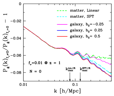
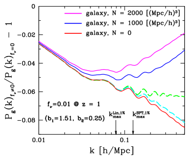
The top panel of Fig. 5 explicitly shows how a scale-dependent bias in the galaxy power spectrum is modeled by $b_{2}$. Note that we consider $z=1$ and $N=0$, and the spectra plotted are divided by $b_{1}^{2}P_{\rm m}(k)$ such that deviation from unity represents the effect of scale-dependent bias. Here we consider $b_{2}=\pm 0.25$ and 1.2 as a working example. First of all, it is worth noting that the nonlinear galaxy bias of $b_{2}\sim 0.1-1$ causes a modification in the galaxy power spectrum shape at BAO scales, and the effect may need to be taken into account for BAO surveys. For a case of $b_{2}<1$, as can be seen from the results of $b_{2}=\pm 0.25$, a positive (negative) $b_{2}$ enhances (suppresses) the power spectrum amplitudes increasingly at larger $k$, relative to the linear bias case. These features are from the second term in the bracket on the r.h.s of Eq. (40) because $P_{\rm b2,\delta}>0$. On the other hand, when $b_{2}>1$, the nonlinear bias causes a complicated modification in the spectrum shape, because the third term in Eq. (40) becomes dominant over the second term at larger $k$. Note that the third term is always negative, so always suppresses the power spectrum amplitudes.

The results in the top panel imply that, even if a linear bias parameter is well determined, the scale-dependent bias may cause a degeneracy with the effect of finite neutrino masses, thereby degrading the ability of future surveys for constraining neutrino masses. In particular a negative $b_{2}$ causes a suppression in the power spectrum amplitudes, similarly to the neutrino effect, so this case may cause a stronger degeneracy. To obtain an insight on this, the middle panel of Fig. 5 studies the neutrino suppression effect on galaxy power spectrum in the presence of nonlinear bias. Shown here is the fractional difference of galaxy spectra with and without neutrinos of $f_{\nu}=0.01$, for three cases of $b_{2}$. For comparison, the dashed curves show the results for “matter” power spectra employing linear theory and SPT. While the neutrino suppression effect is preserved, the nonlinear bias alters the features in the weakly nonlinear regime. This figure shows that a negative (positive) $b_{2}$ weakens (strengthens) the suppression effect.

The bottom panel shows the dependence on the residual shot noise contamination, given by the term including the parameter $N$ in Eq. (40). The shot noise term has no wavenumber dependence for the power spectrum measurement, but the figure implies that the shot noise residual with $N=O(10^{3})~{}({{\rm Mpc}/h})^{3}$ may significantly alter the power spectrum shape over a wide range of wavelengths where the neutrino suppression effect appears. This residual shot noise effect arising from nonlinear clustering can be studied by using semi-analytic $N$-body simulations where galaxies are populated with halos, so may be not so a serious source of systematics in the end (e.g. Smith:2006ne ).

Thus nonlinear bias effects cause additional modification on the galaxy power spectrum shape. Therefore uncertainties in the nonlinear bias parameters need to be properly taken into account in extracting cosmological parameters from the measured power spectrum. These will be carefully studied below.

V Parameter Forecasts

We now estimate the ability of future surveys for constraining neutrino masses when using the SPT model predictions to be compared with the measurements.

V.1 Fisher Matrix Formalism

For an actual galaxy redshift survey, there is another nonlinear effect to be taken into account: redshift distortion effect due to the peculiar velocities of galaxies. The redshift distortion causes the redshift-space power spectrum to be two-dimensional: the galaxy clustering strength is varying as a function of two wavenumbers perpendicular and parallel to the line-of-sight direction. The redshift-space power spectrum would be more prominent than the real-space one to carry useful cosmological information including dark energy parameters because it contains the geometrical distortions in directions both along and perpendicular to the line-of-sight, the so-called Alcock-Paczynski test AP (also see Seo:2003pu ; Matsubara:2002rf ). However the distortion effect in the nonlinear regime is not yet fully understood, and a more careful study based on high-resolution $N$-body simulations is needed to develop the accurate modelling Taruya:2009ir . Hence, in this paper for simplicity we focus on the one-dimensional real-space power spectrum. This roughly corresponds to the monopole power spectrum obtained by averaging the redshift-space power spectrum over the spherical shell of a given wavenumber in radius, in combination with the proper weighting as well as with the Finger-of-God compression algorithm Tegmark:2004 , as developed in Tegmark:2006az ; Eisenstein:2005su . Note that, after the spherical shell average, the residual Kaiser’s effect of redshift distortion Kaiser:1984aa behaves like the linear bias parameter. That is, we include only the nonlinear galaxy bias effect.

We can not measure directly the length scale in real space from the observed galaxy distribution; rather we measure the angular positions of galaxies on the sky, and the radial position in redshift space. To convert the observed position to the real-space position, one needs to assume a reference cosmological model which generally differs from the underlying true cosmology. An incorrect mapping causes an apparent distortion in the measured power spectrum, known as the geometrical distortion Seo:2003pu ; Matsubara:2002rf . Since in this paper we focus on the one-dimensional, real-space power spectrum that is given as a function of wavenumber, the wavenumber estimated from the reference cosmology, $k_{\rm ref}$, is related to the true wavenumber $k$ as

$$k=\frac{D_{V}(z)_{\rm ref}}{D_{V}(z)}k_{\rm ref}$$ (43)

where $D_{V}(z)$ is the effective distance factor accounting for the spherical shell average in redshift space, and is given in terms of the angular diameter distance and the Hubble expansion rate as $D_{V}(z)\propto[D_{A}^{2}(z)/H(z)]^{1/3}$ Eisenstein:2005su . The quantities with subscript “ref” denote the quantities for the reference cosmology. Further taking into account the amplitude shift caused by assuming the reference cosmology, the galaxy power spectrum estimated from a galaxy redshift survey, $P^{\rm est}_{g}$, is related to the true spectrum as

$$P^{\rm est}_{\rm g}(k_{\rm ref})=\frac{D_{V}^{3}(z)_{\rm ref}}{D_{V}^{3}(z)}P_{\rm g}(k,z).$$ (44)

In order to estimate the accuracies of neutrino mass determination, we adopt the Fisher matrix formalism (e.g. see Takada:2005si ). The Fisher formalism gives minimal attainable errors on the parameters by means of a set of observables considered. However, this method becomes inaccurate in a case that only an upper bound on neutrino masses rather than the detection can be obtained for a given survey. In this case we need to take into account the non-Gaussian effect of the likelihood, i.e. a sharp cutoff at $f_{\nu}=0$ in parameter space. A more accurate parameter estimation can be obtained, e.g. by using a Markov-Chain Monte-Carlo based method Perotto:2006rj . The Fisher matrix formalism is sufficient for our purpose, which is to estimate ability of future surveys and to examine the impact of the refined model predictions on parameter estimation compared to the linear theory based method.

The Fisher matrix for the galaxy power spectrum measurement for a given survey is expressed in Tegmark:1997rp as

$$F^{\rm galaxy}_{\alpha\beta}=\sum_{i}\frac{V_{\rm s}(z_{i})}{4\pi^{2}}\int^{k_{\rm max}(z_{i})}_{k_{\rm min}}k^{2}dk~{}\frac{\partial\ln P^{\rm est}_{\rm g}(k;z_{i})}{\partial p_{\alpha}}\frac{\partial\ln P^{\rm est}_{\rm g}(k;z_{i})}{\partial p_{\beta}}\left[\frac{\bar{n}_{\rm g}(z_{i})P^{\rm est}_{\rm g}(k;z_{i})}{\bar{n}_{\rm g}(z_{i})P^{\rm est}_{\rm g}(k;z_{i})+1}\right]^{2},$$ (45)

where $p_{\alpha}$ represents a set of free parameters, $V_{\rm s}(z_{i})$ and $\bar{n}_{\rm g}(z_{i})$ are the comoving survey volume and number density of galaxies, respectively, at $i$-th redshift bin defined as $[z_{i}-\Delta z/2:z_{i}+\Delta z/2]$, and the summation runs over redshift slices. Note that $P_{\rm g}$ is given by Eq. (40) and the argument $k$ in $P_{\rm g}^{\rm est}$ is the reference wavenumber $k_{\rm ref}$ in Eq. (43), but we omitted the subscript for notational simplicity. The partial derivative of the power spectrum with respect to parameter $p_{\alpha}$ is computed by infinitesimally varying the parameter $p_{\alpha}$ around the fiducial model assumed, with other parameters $p_{\beta}(\beta\neq\alpha)$ being kept to the fiducial values, such that the Fisher matrix estimates the parameter accuracies around the fiducial model.

To compute the Fisher matrix for a given survey we need to specify lower and upper wavenumber bounds in the $k$-integration of Eq. (45). We set $k_{\rm min}=10^{-4}~{}h{\rm Mpc^{-1}}$, and have checked that choosing the smaller $k_{\rm min}$ little changes the results. On the other hand, one should be careful in choosing the maximum wavenumber for each redshift slice, $k_{\rm max}(z_{i})$, which needs to be chosen from the range of wavenumbers where the model predictions, linear theory or perturbation theory, are reliable and accurate. One way to determine $k_{\rm max}(z_{i})$ is using $N$-body simulations in comparison with the model predictions. However, high-precision simulations for a MDM model are not yet fully explored (see Brandbyge:2008rv ; Brandbyge:2008js for the recent attempts based on the initial pioneer work Klypin:1992sf ). Here we simply employ the following method for a CDM model in Nishimichi:2008ry to specify $k_{\rm max}(z_{i})$ for each redshift slice:

$$\frac{k_{\rm max}(z_{i})^{2}}{6\pi}\int^{k_{\rm max}(z_{i})}_{0}P^{\rm L}_{\rm m}(q;z_{i})dq=C_{\rm max},$$ (46)

where $P^{\rm L}_{\rm m}$ is the input linear mass power spectrum at redshift $z_{i}$. Since $C_{\rm max}$ is a monotonically increasing function with $k_{\rm max}$, we will study how a choice of $k_{\rm max}$ (or equivalently a choice of $C_{\rm max}$) affects our results. Nishimichi:2008ry carefully showed that, for a CDM model, the SPT results fairly well agree with $N$-body simulations up to a maximum wavenumber corresponding to $C_{\rm max}=0.18~{}(0.3)$ to within up to $\sim 1\%$ (3%) accuracy, while the corresponding valid ranges for linear theory are given by the smaller values $C_{\rm max}=0.06~{}(0.13)$. They also showed that another criterion derived by Jeong:2006xd seems optimistic, where it was proposed that SPT predictions agree well with simulations up to $k_{\rm max}$ given by $\Delta^{2}(k_{\rm max})=\left.k^{3}P(k)/2\pi^{2}\right|_{k=k_{\rm max}}\raisebox{-2.15277pt}{$\>\stackrel{{\scriptstyle\textstyle<}}{{\sim}}\>$}0.4$.

We also comment that the Gaussian error covariance for galaxy power spectrum is assumed in Eq. (45), where the power spectra of different wavenumbers are assumed to be independent. Non-linearities of structure formation cause correlated errors of different band powers, i.e. non-Gaussian errors for power spectrum measurement, due to the nonlinear mode-coupling. The non-Gaussian errors are not negligible even on BAO scales, comparable with neutrino free-streaming scales, and are more significant at higher $k$ due to stronger nonlinearities. However at scales of our interest the impact of non-Gaussian errors on parameter estimation is expected to be insignificant, so we employ the Gaussian error assumption for simplicity (see Takada:2008fn ; Takahashi:2009bq for more detailed studies on the non-Gaussian errors).

A galaxy survey alone cannot determine all the cosmological parameters simultaneously due to severe parameter degeneracies. A useful way to break the parameter degeneracies is combining the galaxy survey constraints with the constraints obtained from CMB temperature and polarization anisotropies. In this paper we include information from the CMB temperature anisotropy, $C_{l}^{\rm TT}$, $E$-mode polarization, $C_{l}^{\rm EE}$, and their cross correlation, $C_{l}^{\rm TE}$, where we use the range of multipoles $10\leq l\leq 1500$ for $C_{l}^{\rm TT}$ and $C_{l}^{\rm TE}$ and use $2\leq l\leq 1500$ for $C_{l}^{EE}$, respectively. To compute the CMB fisher matrix, $\mbox{\boldmath$F$}^{\rm CMB}_{\alpha\beta}$, we adopt the noise per pixel and the angular resolution for the Planck experiment that were assumed in Planck:2006uk .

To model the galaxy power spectra and CMB spectra we include all the key parameters that affect the observables within the CDM and dark energy cosmological framework. Our fiducial model is based on the WMAP 5-year results Komatsu:2008aa : the density parameters for total matter and baryon are $\Omega_{\rm m0}(=0.24)$, $\Omega_{\rm m0}h^{2}(=0.1277)$, and $\Omega_{\rm b0}h^{2}(=0.0223)$ (note that we assume a flat universe); the primordial power spectrum parameters are the spectral tilt, $n_{s}(=1.0)$, the running index, $\alpha_{s}(=0)$, and the normalization parameter of primordial curvature perturbations, $\Delta^{2}_{\cal R}(k_{0})(=2.35\times 10^{-9})$ (the values in the parentheses denote the fiducial model). We employ the transfer function computed from the CAMB code, and note that the primordial spectrum amplitude is normalized at $k_{0}=0.002~{}{\rm Mpc}^{-1}$ following the convention in Komatsu:2008aa . The redshift evolution of dark energy density is given by $\Omega_{\rm de}(=1-\Omega_{\rm m0})$ and the equation of state parameter $w_{0}(=-1)$. When computing the CMB spectra, we further include the Thomson scattering optical depth to the last scattering surface, $\tau(=0.089)$. For neutrino parameters we assume the standard three neutrino species and vary the fiducial value of total neutrino mass, $f_{\nu}$. In summary, for a galaxy surveys with $N_{z}$ redshift slices in combination with the hypothetical Planck constraints, the model parameters we consider are given as

$$p_{\alpha}=\{\Omega_{\rm m0},\Omega_{\rm m0}h^{2},\Omega_{\rm b0}h^{2},w_{0},f_{\nu},n_{\rm S},\alpha_{\rm S},\Delta^{2}_{\cal R},\tau,b_{1}(z_{i}),b_{2}(z_{i}),N(z_{i})\},$$ (47)

where $z_{i}=z_{1},z_{2},....,z_{N_{z}}$. In total, we include $(9+3N_{z})$ free parameters for our Fisher matrix analysis. Note that, for the linear theory analysis for the parameter forecasts, we consider $(9+2N_{z})$ free parameters (the parameters above minus the nonlinear bias parameters $b_{2}(z_{i})$). The fiducial values of galaxy bias and shot noise parameters change with a galaxy survey specification and are described in the next subsection.

The full Fisher matrix for the joint experiment of galaxy survey and CMB can be obtained simply by adding the Fisher matrices: $\mbox{\boldmath$F$}_{\alpha\beta}=\mbox{\boldmath$F$}^{\rm galaxy}_{\alpha\beta}+\mbox{\boldmath$F$}^{\rm CMB}_{\alpha\beta}$. The unmarginalized error on a given parameter $p_{\alpha}$ is given as $\sigma(p_{\alpha})=(F_{\alpha\alpha})^{-1/2}$, which corresponds to the accuracy of determining $p_{\alpha}$ when other parameters are perfectly known. On the other hand, the marginalize error including uncertainties of other parameters is given as $\sigma(p_{\alpha})=[(\mbox{\boldmath$F$}^{-1})_{\alpha\alpha}]^{1/2}$, where $\mbox{\boldmath$F$}^{-1}$ denotes the inverse of the Fisher matrix. The correlation coefficient $r$ between two parameters, $p_{\alpha}$ and $p_{\beta}$, is also useful to study how the parameters are degenerate with each other:

$$r(p_{\alpha},p_{\beta})\equiv\frac{(\mbox{\boldmath$F$}^{-1})_{\alpha\beta}}{\sqrt{(\mbox{\boldmath$F$}^{-1})_{\alpha\alpha}(\mbox{\boldmath$F$}^{-1})_{\beta\beta}}}.$$ (48)

If $r=+1~{}(-1)$, the parameters are totally correlated (anti-correlated), while $r=0$ means no correlation between the two parameters.

V.2 Survey Parameters

Survey	$z_{\rm c}$	$\Delta z$	$\bar{n}_{\rm g}$ $10^{-4}(h^{3}{\rm Mpc}^{-3})$	Survey Area $({\rm deg}^{2})$	$V_{\rm s}$ $(h^{-3}{\rm Gpc}^{3})$	$b_{1}$	$b_{2}$	$N$ $10^{4}(h^{-3}{\rm Mpc}^{3})$	$k^{\rm SPT3\%}_{\rm max}$ $(h{\rm Mpc}^{-1})$	$\bar{n}_{\rm g}P_{\rm g}$ $(k^{\rm SPT3\%}_{\rm max})$
SDSS LRG	0.3	0.2	1.0	10000	1.17	2.10	0.336	0.0778	0.120	1.67
($0.2<z<0.4$)
BOSS	0.45	0.1	3.0	10000	1.13	2.13	0.140	0.0062	0.127	3.94
$(0.4<z<0.7)$	0.55	0.1	3.0	10000	1.53	2.21	0.211	0.0125	0.133	3.57
	0.65	0.1	3.0	10000	1.94	2.29	0.263	0.0194	0.138	3.27
Stage-III low-$z$	0.8	0.2	4.0	3200	1.61	1.41	0.295	0.0177	0.146	1.31
	1.0	0.2	4.0	3200	2.06	1.51	0.443	0.0332	0.158	1.15
$(0.7<z<1.6)$	1.2	0.2	4.0	3200	2.42	1.63	0.572	0.0524	0.170	1.07
	1.45	0.3	4.0	3200	4.15	1.77	0.760	0.0851	0.184	0.97
Stage-III high-$z$	2.9	0.8	$2.5$	300	1.23	3.30	2.215	0.2719	0.275	0.43
($2.5<z<3.3$)
Stage IV	0.6	0.2	200	20000	6.94	1.31	-0.409	0.0124	0.134	69.4
	0.8	0.2	200	20000	10.07	1.41	-0.384	0.00933	0.146	57.2
	1.0	0.2	200	20000	12.85	1.51	-0.345	0.00594	0.158	49.3
	1.2	0.2	200	20000	15.14	1.63	-0.299	0.00383	0.170	45.5
($0.5<z<2.1$)	1.4	0.2	200	20000	16.94	1.74	-0.242	0.00217	0.182	40.4
	1.6	0.2	200	20000	18.29	1.86	-0.177	$9.96\times 10^{-4}$	0.195	34.8
	1.8	0.2	200	20000	19.27	1.99	-0.096	$2.38\times 10^{-4}$	0.206	31.2
	2.0	0.2	200	20000	19.94	2.11	-0.016	$0.06\times 10^{-4}$	0.219	28.4

Table 1: Survey parameters that we assume in this paper to make parameter forecasts. The survey parameters are chosen such that the surveys fairly well represent the existing survey (SDSS LRG), the near-future planned survey (BOSS), and the 5-10 year time-scale future surveys which we call Stage-III and -IV surveys, respectively, according to Dark Energy Task Force Report Albrecht:2006um . We employ the method described in Appendix D (also see text) in order to determine the fiducial values of the linear and nonlinear bias parameters $b_{1}$ and $b_{2}$ for each redshift slice of the respective survey. We also include the residual shot noise contamination arising from nonlinear clustering, which is parametrized by $N$, and we determine the fiducial value of each redshift slice according to the method in Appendix D. The values in the column labelled by $k_{\rm max}^{\rm SPT3\%}$ denote the maximum wavenumber up to which the standard perturbation theory (SPT) is expected to be reliable to within a few $\%$ accuracy compared to $N$-body simulation results at each redshift (we determined the $k_{\rm max}$ values following using Eq. 46). We also show the quantity $\bar{n}_{\rm g}P_{\rm g}(k_{\rm max})$ at the maximum wavenumber for each redshift slice: if $\bar{n}_{\rm g}P_{\rm g}(k_{\rm max})\geq 1$, the power spectrum measurement is in the sample variance limited regime.

To make meaningful parameter forecasts, we consider survey parameters that fairly well represent future surveys being planned or under serious consideration. The hypothetical surveys considered in this paper are intended to resemble BOSS, WFMOS-like survey, and the ideal space-based BAO experiment such as those proposed by JDEM and Euclid missions, which are roughly categorized as the Stage-III and -IV surveys, respectively, in the DETF report Albrecht:2006um .

The survey parameters are summarized in Table 1. The survey area, redshift range and number densities of target galaxies were taken from the proposed survey design of each survey. Just briefly, the BOSS-like survey samples luminous red galaxies (LRGs) over a range of redshifts $0.4<z<0.7$ extending the SDSS-I and -II surveys. A ground-based Stage-III survey with optical spectroscopy may be designed to survey galaxies for two different slices: one is for galaxies over $0.7<z<1.6$ with survey area $3200$ deg², and the other is for high-redshift Lyman-$\alpha$ emission or Lyman break galaxies over $2.5<z<3.3$. The survey parameters for the Stage-IV type survey are taken from bennet . Having multiple redshift slices is useful to improve the accuracies of parameter estimation by breaking the parameter degeneracies because the sensitivity of each redshift slice to cosmological parameters is slightly different as will be shown below (also see Matsubara:2004 for the related discussion). These surveys are complementary to each other in redshift ranges covered. It is also worth commenting that a high-redshift survey with $z>1$ has a potential to explore an early dark energy model where dark energy may be more rapidly evolving at higher redshifts than naively expected.

We further need to specify galaxy bias parameters. However, because we have a limited knowledge on galaxy formation, it is difficult to predict galaxy bias parameters with certainty. Here we rather employ a crude method used in Seo:2003pu ; Takada:2005si to estimate the linear galaxy bias parameter $b_{1}$ for each redshift slice, where $b_{1}$ is estimated by imposing the rms number density fluctuations of galaxies within a sphere of $8h^{-1}$Mpc radius to be unity: $\sigma_{g8}^{2}=1$. However the LRG bias is relatively well understood based on the existing SDSS sample such as $b_{1}\approx 2.1$ in Tegmark:2006az . We assume $b_{1}=2.1$ for the fiducial value of SDSS LRG bias, from which we compute a correction factor that needs to be multiplied by $\sigma_{g8}^{2}=1$ to obtain $b_{1}=2.1$ for our fiducial cosmological model. Similarly, for BOSS LRGs, we multiply $\sigma_{g8}^{2}=1$ by the same correction factor to estimate the linear bias $b_{1}$ (see Appendix D for more details). The nonlinear bias parameter $b_{2}$ and the residual shot noise parameter $N$ are more uncertain. We define their fiducial values based on the prescription described in Appendix D, but will study how our results change with different fiducial values of $b_{2}$ and $N$. Note that the parameter $N$ is estimated based on the perturbation theory, but we will employ the same fiducial value for the linear theory based forecasts. When $N\geq 1/\bar{n}_{\rm g}$, the residual shot noise contamination is dominant. Our survey parameters imply that, for BOSS and Stage-III surveys, $N<1/\bar{n}_{\rm g}$. On the other hand, the residual shot noise contamination is significant for some redshift slices having higher number densities of galaxies for the Stage-IV survey.

V.3 Parameter Forecasts

V.3.1 Summary of constraints on neutrino mass

Expected marginalized error on total neutrino mass: $\sigma(m_{\nu,{\rm tot}})$ (eV) Survey     Linear 1% $C_{\rm max}=0.06$        Linear 3% $C_{\rm max}=0.13$        SPT 1% $C_{\rm max}=0.18$        SPT 3% $C_{\rm max}=0.3$        + $\sigma(\Omega_{\rm m0})=0.01$ $C_{\rm max}=0.3$ BOSS 0.161 0.111 0.095 0.088 0.082 Stage-III (low-z slices alone) 0.173 0.123 0.110 0.096 0.082 Stage-III (low- + high-z) 0.161 0.122 0.107 0.091 0.081 Stage IV 0.067 0.059 0.053 0.046 0.046

Table 2: Marginalized 1$\sigma$ error on total neutrino masses, $\sigma(m_{\nu,{\rm tot}})~{}[{\rm eV}]$, expected from each hypothetical survey when combined with the Planck and $z\sim 0.3$ SDSS LRG information. The errors are derived including the galaxy power spectrum information over $10^{-4}\leq k\leq k_{\rm max}~{}h{\rm Mpc}^{-1}$, where $k_{\rm max}$ is determined by Eq. (46) from the input linear mass power spectrum. As implied, the linear theory and perturbation theory are expected to be accurate up to the given $k_{\rm max}$ to within a given $\%$ accuracy compared to $N$-body simulations Nishimichi:2008ry . For these results we assume $m_{\nu,{\rm tot}}=0.12{\rm eV}~{}(f_{\nu}=0.01)$ for the fiducial value of neutrino mass, therefore the errors shown roughly correspond to the expected $1\sigma$ upper limit on neutrino mass if $\sigma(m_{\nu,{\rm tot}})\raisebox{-2.15277pt}{$\>\stackrel{{\scriptstyle\textstyle>}}{{\sim}}\>$}0.12~{}{\rm eV}$. The last column labelled by “$+\sigma(\Omega_{\rm m0})=0.01$” shows an improvement in the neutrino mass constraint for the case $C_{\rm max}=0.3$ if the prior $\sigma(\Omega_{\rm m0})=0.01$ is added.

Table 2 summarizes forecasts for the marginalized errors on total neutrino mass for each of hypothetical galaxy surveys listed in Table 1, combined with the Planck and SDSS LRG information. To derive these errors we determined $k_{\rm max}$ for each redshift slice based on the criteria (46) and then included the power spectrum information over $10^{-4}\leq k\leq k_{\rm max}(z_{i})~{}h\rm{Mpc}^{-1}$. We compare the expected constraints obtained when using the linear theory and SPT models, over a range of wavenumbers where the respective models seem reliable as indicated from the assumed value of $C_{\rm max}$ (the corresponding $k_{\rm max}$ values when $C_{\rm max}=0.3$ for each redshift slice are listed in Table 1). Note that we assume $f_{\nu}=0.01$ ($m_{\nu,{\rm tot}}\simeq 0.12~{}{\rm eV}$) for the fiducial value, and the number of free parameters is different in between the linear theory and SPT as described around Eq. (47) (SPT additionally includes the nonlinear bias parameter $b_{2}$ for each redshift slice).

It is clear that the use of SPT allows for an improvement in the neutrino mass constraint compared to the linear theory results: roughly a factor of 1.3 improvement if SPT can be used up to the maximum wavenumbers where SPT seems reliable to within a few % accuracy corresponding to $C_{\rm max}=0.3$. We have checked that the accuracy of neutrino mass determination, $\sigma(m_{\nu,{\rm tot}})$, little changes for each survey even if the fiducial value of $f_{\nu}$ is varied within the current limit $f_{\nu}\raisebox{-2.15277pt}{$\>\stackrel{{\scriptstyle\textstyle<}}{{\sim}}\>$}0.05$. Hence Table 2 implies the BOSS and Stage-III type survey may allow for the accuracy of $\sigma(m_{\nu,{\rm tot}})\simeq 0.1~{}$eV, while the Stage-IV survey $\sigma(m_{\nu,{\rm tot}})\simeq 0.05~{}$eV. In particular the expected accuracy for a Stage-IV type survey is compatible with the lower limit implied from the normal mass hierarchy. That is, Stage-IV may allow for a detection of total neutrino mass at more than $1$-$\sigma$ significance; if neutrinos obey the inverted mass hierarchy implying the lower limit $m_{\nu,{\rm tot}}\raisebox{-2.15277pt}{$\>\stackrel{{\scriptstyle\textstyle>}}{{\sim}}\>$}0.1~{}$eV, a 2-$\sigma$ level detection may be achieved.

Note that the forecasted constraints here are much weaker than those obtained in our previous work Saito:2008bp . The differences are (1) we here consider the one-dimensional power spectrum as the observable rather than the full two-dimensional power spectrum in redshift space and (2) we include the nonlinear bias parameters. The full analysis including the two-dimensional redshift power spectrum information will be presented elsewhere (Saito et al. in preparation).

V.3.2 Degeneracy between neutrino mass and other parameters

To develop a better understanding of the forecasted neutrino mass errors, we study how parameters are degenerate with each other and how the degeneracies can be broken when the galaxy power spectrum information ranging from the linear to non-linear regime are combined with the CMB information. First, the top panel of Fig. 6 shows the unmarginalized errors on neutrino mass as a function of the maximum wavenumber, for the single $z=1$ slice of the Stage-III low-$z$ survey in Table 1, where the linear theory result is compared with the SPT results obtained assuming various fiducial values of nonlinear bias parameter $b_{2}$. For $k_{\rm max}\raisebox{-2.15277pt}{$\>\stackrel{{\scriptstyle\textstyle<}}{{\sim}}\>$}0.07~{}h{\rm Mpc}^{-1}$, the neutrino mass constraint does not depend on $k_{\rm max}$, implying that the constraint is mostly from the CMB information. For the larger $k_{\rm max}$ the galaxy power spectrum is becoming to be more powerful to constrain the neutrino mass due to the increased independent Fourier modes. From comparison between the linear theory and SPT results, one can find that the unmarginalized error on neutrino mass is improved in the weakly nonlinear regime due to the improved signal-to-noise ratio of power spectrum measurement, except for the case of $b_{2}<0$. The case of $b_{2}<0$ causes a suppression in the power spectrum amplitudes, as implied in the top panel of Fig. 5. As a result the information content of the power spectrum does not increase so much in the weakly nonlinear regime compared to the linear theory, although the linear theory breaks down in the regime. Thus the neutrino mass constraints are sensitive to galaxy bias parameters or equivalently galaxy types.

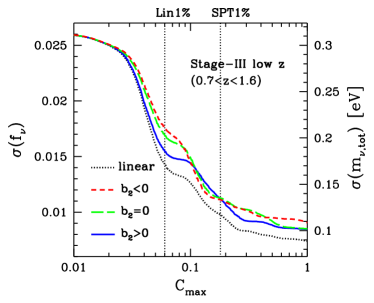
The upper-right panel shows the neutrino mass errors marginalized over other parameter uncertainties. Again notice that the results are only for one $z=1$ slice of the Stage-III low-$z$ survey corresponding to the survey volume $2.1~{}h^{-3}{\rm Gpc}^{3}$ (see below for the full forecast for all the redshift slices combined). Compared to the unmarginalized errors, the neutrino mass error is significantly degraded due to strong parameter degeneracies. The plot also shows a clear plateau feature in the error for $k_{\rm max}\raisebox{-2.15277pt}{$\>\stackrel{{\scriptstyle\textstyle<}}{{\sim}}\>$}0.1~{}h{\rm Mpc}^{-1}$, and then shows a step-like improvement in the error at some particular $k_{\rm max}$ values, which are found to correspond to the BAO peaks. Namely, when the BAO peaks are included by increasing $k_{\rm max}$, the accuracies of constraining cosmological parameters are dramatically improved by breaking the parameter degeneracies via the Alcock-Paczynski test. Comparing the linear theory and SPT results manifests that, in contrast to the results for the unmarginalized errors, the neutrino mass error does not improve by using SPT, due to the significant parameter degeneracies and the addition of nonlinear bias parameter $b_{2}$. The effect of $b_{2}$ can be explicitly studied by the dot-dashed curve, where $b_{2}$ is kept fixed. Fixing $b_{2}$ does improve the neutrino mass constraints, implying a strong degeneracy between neutrino mass and $b_{2}$ in the nonlinear power spectrum. However, the SPT result with $b_{2}$ being fixed is still apparently worse than the linear theory extrapolated result in the weakly nonlinear regime (although the linear theory breaks down in the regime). This may be understood as follows. As discussed, the neutrino mass constraints are sensitive to an inclusion of BAO features which helps break parameter degeneracies. However, the nonlinear mode coupling somewhat smooths out BAO features in the weakly nonlinear regime, which degrades the constraining power of galaxy surveys in the weakly nonlinear regime.

The bottom panel of Fig. 6 explicitly studies the Fisher correlation coefficients of neutrino mass with other parameters, $r(f_{\nu},p_{\alpha})$, as a function of $k_{\rm max}$ for the $z=1$ slice. The neutrino mass appears to be significantly degenerate with some parameters such as $\Omega_{\rm m0}h^{2}$, $w_{0}$, $\Omega_{\rm m0}$ and $b_{2}$ showing almost perfect degeneracy of $|r|\sim 1$. The degeneracies show complex behaviors as a function of $k_{\rm max}$, where the oscillatory features of $r$ correspond to the BAO features.

We comment on the parameter $N$ which models the residual shot noise contamination to the power spectrum measurement due to nonlinear clustering of galaxies. For the assumed Stage-III survey, the residual shot noise contamination arising from the nonlinear galaxy clustering is smaller than the standard shot noise $1/\bar{n}_{\rm g}$. In addition the sample variance gives a dominant contribution to the power spectrum covariance over all the scales we consider, $k\raisebox{-2.15277pt}{$\>\stackrel{{\scriptstyle\textstyle<}}{{\sim}}\>$}0.3~{}h{\rm Mpc}^{-1}$. Therefore the effect of $N$ is insignificant for the results shown here. However, the genuine effect needs to be studied using $N$-body simulations, since this shot noise contamination is not yet fully explored.

Figure 6: Top-left panel: The unmarginalized $1\sigma$ error on $f_{\nu}$ as a function of the maximum wavenumber $k_{\rm max}$, expected from a single redshift slice around the centering redshift $z_{\rm c}=1$ of Stage-III low-$z$ survey in Table 1. The short-dashed, long-dashed and solid curves show how the neutrino mass error changes if the nonlinear bias parameter is changed from the fiducial choice $b_{2}=0.443$ to the other choices $b_{2}=-0.443$ and 0, where other survey parameters are fixed as shown in Table 1. The neutrino mass constraint is sensitive to the underlying $b_{2}$, i.e. galaxy types. For comparison, the dotted curve shows the linear theory result. Note that the two vertical dotted lines show the maximum wavenumbers up to which the perturbation theory is expected to be accurate to within the given accuracy for this redshift slice. Top-right panel: The similar plot, but shows the marginalized errors on neutrino mass. The step-like features are apparent: the plateau shape is due to strong parameter degeneracies and a sudden drop of the error at some particular wavenumbers imply an improvement in the parameter errors because the parameter degeneracies can be to some extent broken by including the BAO features with increasing $k_{\rm max}$. Compared to the top-left panel, the marginalized error is not necessarily more stringent in the weakly nonlinear regime than the linear theory extrapolated error due to the stronger parameter degeneracies, although the linear theory ceases to be reliable in the nonlinear regime. Bottom panel: The correlation coefficients of neutrino mass with other parameters, $r(f_{\nu},p_{\alpha})$, defined by Eq. (48), displaying complex degeneracy behaviors as a function of $k_{\rm max}$.

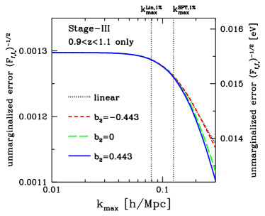
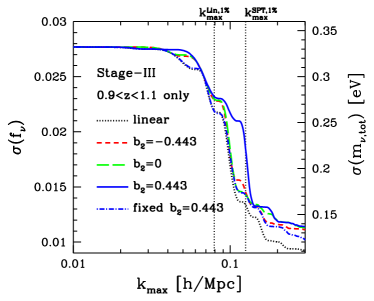
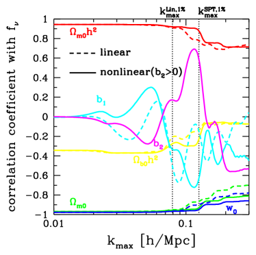
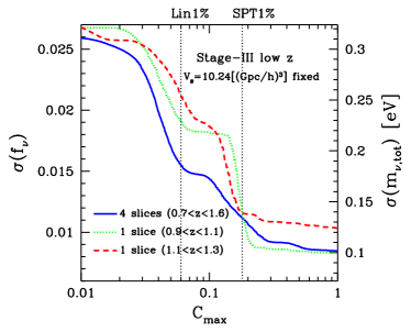
Fig. 7 shows the results combining all the four redshift slices for Stage-III low-$z$ survey (the total survey volume $V_{s}=10.24~{}h^{-3}{\rm Gpc}^{3}$). The left panel demonstrates the marginalized errors on neutrino mass as in Fig. 7, but as a function of $C_{\rm max}$, where $k_{\rm max}$ for each redshift slice is specified by using Eq. (46). Compared to Fig. 5, the accuracies of neutrino mass determination continue to improve with increasing $k_{\rm max}$ or adding more galaxy power spectrum information; there is no regime dominated by CMB information over the scales we have considered. This is because the galaxy power spectra at different redshifts depend on cosmological parameters in different ways, so combining the different redshift information helps break the parameter degeneracies. The solid, short- and long-dashed curves compare the results for different fiducial values of $b_{2}$: In the first case we adopt the fiducial values of $b_{2}$ given in Table 1, while in the second case we multiply the minus sign in the fiducial values of $b_{2}$ in Table 1 (all the $b_{2}$ values are negative for this case). In the third one, we set $b_{2}=0$ for all redshift slices. As also discussed in Fig. 5, the neutrino mass determination accuracies are found to be sensitive to the fiducial values of $b_{2}$, or equivalently to galaxy types targeted for future surveys. However the differences due to different values of $b_{2}$ become milder by combining different slices.

The SPT results can be compared with the linear theory result (the dotted curve). As in Fig. 5, the nonlinear regime suffers from severe parameter degeneracies, yielding less stringent parameter constraints than naively expected by linear theory. For this reason the parameter forecasts in the previous studies may be somewhat too optimistic, if the forecasts are derived based on the linear theory and the linear bias parameter (e.g., Takada:2005si ; Hannestad:2007cp ; Saito:2008bp ). However, we again note that the full information on galaxy clustering is inherent in the two-dimensional redshift space, while we consider the one-dimensional power spectrum in this paper.

The usefulness of combining different redshift slices is explicitly shown in the right panel of Fig. 7. The plot compares between the results of different redshift slicing, where the survey volume is kept fixed to $V_{s}\simeq 10.24~{}h^{-3}{\rm Gpc}^{3}$. However, note that the maximum wavenumber $k_{\rm max}$ is different for different redshift slices, therefore the effective survey volume is different. The solid curve is the result of our fiducial Stage-III low-$z$ survey, while the dotted and dashed curves are the results assuming single redshift slice which have different centering redshifts $z_{c}=1.0$ and $1.2$ with width $\Delta z=0.2$, respectively. The single redshift slice cases correspond to survey areas $\Omega_{\rm s}=15900$ and $13500$ deg², respectively, compared to the fiducial area $\Omega_{\rm s}=3200$ deg² over redshift range $0.7\leq z\leq 1.6$. It is clear that the neutrino mass constraint is improved by combining the different redshift slices. Also, comparing the dotted and dashed curves clarifies that a choice of redshift slices affects the constraining power in the weakly nonlinear regime.

V.3.3 Impact of massive neutrinos on dark energy constraints

Figure 7: Left panel: As in the top-right panel of the previous figure, this plot shows the marginalized error on $f_{\nu}$ obtained by combining the four different redshift slices of Stage-III low-$z$ survey in Table 1 as a function of $C_{\rm max}$, where the maximum wavenumber of each redshift slice, $k_{\rm max}(z_{i})$, is computed using Eq. (46) for an input $C_{\rm max}$ given in the horizontal axis. Note that for reference $C_{\rm max}=0.1~{}(1.0)$ corresponds to $k_{\rm max}=0.097~{}(0.266)~{}h{\rm Mpc}^{-1}$ at $z=1$. The fiducial values of nonlinear bias parameters $b_{2}$ for each redshift slice, which are all positive, are given in Table 1. For comparison, the short- and long-dashed curves show the results obtained when the sign of $b_{2}$ is flipped or assuming $b_{2}=0$ for all the slices, respectively. Right panel: The complementarity of different redshift slices is more explicitly studied. The solid curve is same as the solid curve in the left panel. The dotted and dashed curves show the results for only one redshift slice with the centering redshifts $z_{c}=1$ and $1.2$, respectively, keeping the survey comoving volume fixed.

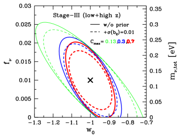
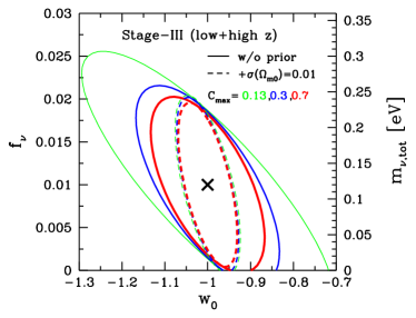
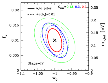
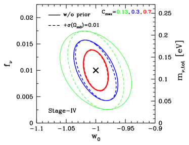
The primary science goal of future surveys is constraining the nature of dark energy via the BAO experiment. However, the dark energy constraints may be biased if the model fitting ignores neutrino mass contribution. Fig. 8 presents the marginalized error ellipses in a sub-space of the neutrino mass $f_{\nu}$ and the dark energy equation state parameter $w_{0}$ for the Stage-III and -IV surveys, respectively. Note that the dark energy constraints shown here are from both the BAO peak locations and the power spectrum amplitude information. There appears to be a significant correlation between $w_{0}$ and neutrino mass as expected. For example, a model with $w_{0}>-1$ or greater $\Omega_{\rm de0}$ yields smaller amplitudes in the galaxy power spectrum, because such a model causes dark energy to be more significant from earlier epochs and therefore the greater cosmic acceleration suppresses the clustering growth rate for the CMB normalization of linear power spectrum amplitude. This dark energy effect can be compensated by lowering the neutrino mass (i.e. the smaller $f_{\nu}$) that leads to a less suppression in the power spectrum amplitudes at the larger $k$. One can also find that having larger $k_{\rm max}$ (equivalently larger $C_{\rm max}$) yields more stringent constraints on these parameters. In particular, it should be noted that a Stage-IV type survey may allow for a stringent test of neutrino mass, even from the 1D power spectrum information over a range of wavenumbers where SPT seems reliable.

In Fig. 8 we also study how the parameter constraints are improved by adding an external prior of $b_{2}$ or $\Omega_{\rm m0}$. These priors may be delivered from the galaxy bispectrum analysis Sefusatti:2007 , the SN survey and/or weak lensing surveys Takada:2008fn . Adding the priors shrinks areas of the error ellipses, because $\Omega_{\rm m0}$ and $b_{2}$ are degenerate with neutrino mass and dark energy parameters in the galaxy power spectrum as implied in Fig. 6. In particular, for a Stage-III type survey, the prior of precision $\sigma(\Omega_{\rm m0})\sim 0.01$ can efficiently break the $m_{\nu,{\rm tot}}$-$w_{0}$ degeneracy, thereby yielding the accuracies of $\sigma(m_{\nu,{\rm tot}})\simeq 0.1~{}$eV and $\sigma(w_{0})\simeq 0.05$, respectively. For a Stage-IV type survey, the constraining power is already sufficient, so such a prior does not much help improve the parameter constraints.

Figure 8: Forecasted $1\sigma$ error ellipses in $(w_{0},f_{\nu})$-subspace for Stage-III (top two panels) and Stage IV (bottom), respectively. The outermost, intermediate and innermost contours show the results assuming $C_{\rm max}=0.13$, $0.3$ and $0.7$, respectively, that correspond to the higher $k_{\rm max}$ in each redshift slice. Again note that $C_{\rm max}=0.13$ and 0.3 roughly correspond to the maximum wavenumbers that the linear theory and SPT are reliable with a few % accuracy. The case of $C_{\rm max}=0.7$ may be feasible if the refined model of nonlinear power spectrum can be used (see text for the details). The dashed contours show the errors when the prior of $\sigma(b_{2})=0.01$ (left panels) or $\sigma(\Omega_{\rm m0})=0.01$ (right panels) is added.

A more important question is how the uncertainty of neutrino mass affects dark energy constraints from future galaxy surveys. Table 3 addresses this issue. First, comparing between the third and fourth columns clarifies that the accuracy of $w_{0}$ determination is affected by including neutrino mass parameter in the model fitting. If neutrino mass is ignored, the error of $w_{0}$ is apparently tightened by a factor of 1.2–1.4 for the galaxy surveys we consider here. It should be noted that the tighter constraints correspond to a case that the neutrino mass is sufficiently well determined by a laboratory experiment (i.e. in this case $f_{\nu}$ is no longer a free parameter in the galaxy power spectrum).

More importantly, ignoring neutrino mass in the model galaxy power spectra likely results in a biased best-fit value of $w_{0}$. According to the method described in Appendix E, the column labelled as “$\delta w_{0}$ ignoring $f_{\nu}$” estimates an amount of the possible bias, that is, the difference between the input $w_{0}$ and the best-fit value obtained from the model fitting without neutrino mass parameter: $w_{0}^{\rm best-fit}=-1+\delta w_{0}$. To be more explicit, we here estimate the bias caused when the template of galaxy power spectrum assuming $f_{\nu}=0$ is fitted to the observed spectrum having the true neutrino contribution of $f_{\nu}=0.01$ ($m_{\nu,{\rm tot}}=0.12$ eV). The table shows a positive bias $\delta w_{0}$: $w_{0}^{\rm best-fit}>w_{0}^{\rm input}=-1$, because a model with $w_{0}>-1$ predicts galaxy spectra with smaller amplitudes due to the suppressed growth rate, which mimics the neutrino suppression effect inherent in the (presumably here) measured spectrum. For BOSS and Stage-III type surveys, the bias is not significant because $|\delta w_{0}/\sigma(w_{0})|<1$, while a Stage-IV type survey may suffer from a significant bias as $|\delta w_{0}|\sim\sigma(w_{0})$. Table 3 also shows that a $1\%$-level prior of $\Omega_{\rm m0}$ helps reduce the statistical error $\sigma(w_{0})$, but also make the systematic bias more significant at the same time.

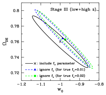
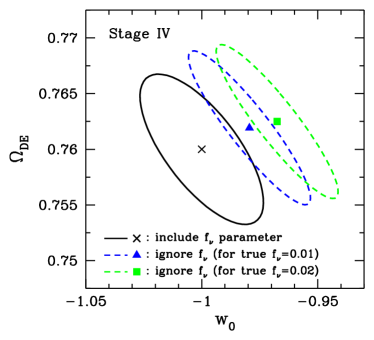
Fig. 9 more nicely illustrates the impact of neutrino mass uncertainty on dark energy parameter estimation from future galaxy surveys, showing the projected error ellipses in ($w_{0},\Omega_{\rm de0}$)-plane. It is clear that ignoring $f_{\nu}$ leads to model fitting apparently with smaller error ellipses and biased best-fit values for these parameters. In particular, for a Stage-IV type survey, the biased best-fit dark energy model confined by the 1-$\sigma$ statistical error bounds may happen to be outside from the underlying true model (the input value $w_{0}=-1$ in our case). The amount of bias would become greater for the greater values of true neutrino mass. Thus Table 3 and Fig. 9 imply that neutrino mass contribution is not negligible and needs to be included in the model interpretation for future galaxy surveys in order not to have too optimistic and biased dark energy constraints.

Note that the parameter biases studied here are mainly from the power spectrum amplitude information. If the dark energy parameters are estimated from BAO peak locations being marginalized over a sufficient number of nuisance parameters that include power spectrum amplitude parameters Seo:2008yx , the dark energy parameter biases can be minimized, although the constraining power is significantly weakened. This is beyond the scope of this paper, but would be worth carefully studying.

Survey	range of $k$ $(C_{\rm max})$	$\sigma(w_{0})$	$\sigma(w_{0})$ ignoring $f_{\nu}$	$\delta w_{0}$ ignoring $f_{\nu}$	$\sigma(w_{0})$ +$\sigma(\Omega_{\rm m0})=0.01$	$\delta w_{0}$ +$\sigma(\Omega_{\rm m0})=0.01$
BOSS	Linear 3% (0.13)	0.1522	0.0978	0.0090	0.0507	0.0262
	SPT 3% (0.30)	0.0768	0.0603	0.0141	0.0435	0.0243
Stage-III	Linear 3% (0.13)	0.1935	0.1067	0.0060	0.0503	0.0255
	SPT 3% (0.30)	0.1103	0.0801	0.0125	0.0476	0.0254
Stage-IV	Linear 3% (0.13)	0.0398	0.0375	0.0113	0.0311	0.0176
	SPT 3% (0.30)	0.0245	0.0223	0.0206	0.0226	0.0223

Table 3: The impact of massive neutrinos on determination of dark energy equation of state parameter, $w_{0}$. Note that $f_{\nu}=0.01$ is assumed for the fiducial model. The fourth and fifth columns, labelled as “ignoring $f_{\nu}$”, show apparently tighter constraints and biased best-fit values of $w_{0}$ caused when galaxy power spectrum models without neutrino mass parameter is fitted to the true spectrum with $f_{\nu}=0.01$, respectively, for each galaxy surveys. The sixth and seventh columns, labeled as “+$\sigma(\Omega_{\rm m0})=0.01$”, show the similar results when adding the prior $\sigma(\Omega_{\rm m0})=0.01$.

Figure 9: The projected $1\sigma$ error ellipses in $(w_{0},\Omega_{\rm DE})$-plane for Stage-III (left panel) and Stage-IV surveys (right panel), respectively. Note that $C_{\rm max}=0.3$ is assumed. The solid contours in each panel shows the result for our fiducial method where neutrino mass contribution to the galaxy power spectrum is properly taken into account and the errors on dark energy parameters are derived by marginalizing over other parameter uncertainties. The dashed contours and the triangle or square symbols show the worst-case results: apparently tighter constraints (smaller error ellipses) and biased best-fit values may be caused if neutrino mass contribution is ignored in the model galaxy power spectra. The triangle and square symbols show the biased values when the underlying true cosmology has $f_{\nu}=0.01$ ($m_{\nu,{\rm tot}}=0.12$ eV) and $0.02$ (0.24 eV), respectively. For a Stage-IV type survey, ignoring neutrino mass may cause a false best-fit model that is away from the true model $w_{0}=-1$ by more than the 1-$\sigma$ statistical errors.

VI Summary and discussion

Following our earlier work Saito:2008bp , in this paper we have developed a method for computing nonlinear power spectra of total matter and galaxies in a mixed dark matter (MDM) model (a model with CDM plus finite-mass neutrinos) based on standard perturbation theory (SPT) approach. In particular we have carefully examined the validity of approximations employed in our approach.

For our fiducial approach, we include only the linear-order neutrino perturbations to compute the nonlinear power spectrum, where nonlinear clustering is driven by the nonlinear growth of CDM plus baryon perturbations. Our approach is motivated by the fact that the neutrino free-streaming scale is sufficiently large for small neutrino mass scales consistent with the current limit ($m_{\nu,{\rm tot}}\raisebox{-2.15277pt}{$\>\stackrel{{\scriptstyle\textstyle<}}{{\sim}}\>$}0.6$ eV) and the neutrinos are expected to more stay in the linear regime than CDM plus baryon. We carefully studied the validity of this assumption as briefly summarized in the following (see Appendix A). By solving the hierarchical Boltzmann equations of neutrino perturbations including the nonlinear gravitational potential contribution (due to the nonlinear CDM and baryon density perturbations), we indeed found that the amplitudes of neutrino density perturbations are enhanced by up to $10\%$ at the weakly nonlinear scales up to $k\sim 0.5$Mpc^-1. Thus, although the neutrino perturbation is indeed affected by nonlinear clustering, the contribution to total matter power spectrum can be safely ignored to less than a sub-percent level, for neutrino mass scales of interest, because the neutrino perturbation contribution to total matter clustering is suppressed by another small factor $f_{\nu}=\Omega_{\nu 0}/\Omega_{\rm m0}$ whose current limit $f_{\nu}\raisebox{-2.15277pt}{$\>\stackrel{{\scriptstyle\textstyle<}}{{\sim}}\>$}0.05$.

Further we carefully studied the higher-order growth functions of CDM plus baryon perturbations. Compared to the CDM case, the finite-mass neutrinos cause a scale-dependent suppression in the clustering growth rate, and therefore the higher-order growth rates generally have complicated scale dependence. That is, the additional nonlinear mode-coupling between perturbations of different wavenumbers arise via the growth rates in a MDM model. We numerically solved the differential equations of the higher-order growth rates, and found that the higher-order growth rates are well approximated by the power of the linear growth rate (see Fig. 1).

As a result the nonlinear power spectra can be approximately given by rather simple forms (see Eqs.[32], [36] and [37]) similarly as in the SPT approach for a CDM model. The equation (37) is very useful in a sense that the nonlinear power spectrum at a given redshift $z$ can be computed from the linear transfer functions of CDM, baryon and neutrino perturbations at the redshift $z$, which are standard outputs of the publicly available codes, CMBFAST or CAMB. As in Saito:2008bp , we found that the neutrino suppression effect on the total matter power spectrum amplitude is enhanced in the weakly nonlinear regime than in the linear regime (see Fig. 4). Note that the empirical halofit approach shows $10\%$-level deviations from the SPT results in the weakly nonlinear regime, although it qualitatively captures the neutrino effect in the nonlinear regime (see Fig.3).

Thus we believe that our approach gives reliable, accurate model predictions for the nonlinear matter power spectrum in a MDM model over a wider range of scales, where the perturbation theory is valid, than the linear theory. Also important is the SPT approach can explicitly tell the scales and redshifts where the linear theory ceases to be accurate or breaks down. However, simulation based studies are definitely needed to test and/or calibrate the SPT predictions. An $N$-body simulations for a MDM model is still challenging, but encouragingly the initial attempts are being explored in Brandbyge:2008rv ; Brandbyge:2008js . Alternative approach to refine the analytical modeling is to extend the SPT approach by including higher-order loop corrections. Recently there are several efforts made in this direction for a CDM model: the Time-RG formalism Pietroni:2008jx , the renormalized perturbation theory (RPT) Crocce:2007dt and the closure theory approach Taruya:2007xy some of which show remarkable agreement with $N$-body simulations over a wide range of BAO scales Carlson:2009it ; Taruya:2009ir . For example, an attempt to extend the PT approach for a MDM model has recently been made in the framework of the Time-RG formalism Lesgourgues:2009am . Given the similarity between our approach and the PT of CDM model as described above, we hope that our method can be straightforwardly extended to the improved nonlinear modeling. This is our future project, and will be presented elsewhere.

Another interesting result of this paper is we developed a method to compute the nonlinear galaxy power spectrum in a MDM model by taking into account the nonlinear biasing effect in a self-consistent manner within the SPT framework. As given by Eq. (40), the nonlinear galaxy power spectrum is modeled, in addition to cosmological parameters, by introducing the linear and nonlinear bias parameters, $b_{1}$ and $b_{2}$, and one additional parameter to model the residual shot noise contamination $N$. Once again, although the validity of SPT approach needs to be tested by simulations, our SPT approach is built on the physical foundation of large-scale structure formation and therefore expected to be reasonably accurate in the weakly nonlinear regime where the SPT approximately works out.

After formulating the nonlinear galaxy power spectrum, we then estimated the ability of future galaxy surveys for constraining neutrino masses from the power spectrum information over scales ranging from the linear regime to the weakly nonlinear regime. In this paper for simplicity we focused on the real-space power spectrum, i.e. ignored the redshift distortion effect, because the nonlinear distortion effect, the Finger-of-God effect, is not yet fully understood even in the weakly nonlinear regime. We found that the accuracy of neutrino mass constraint is indeed improved by including the power spectrum information up to the weakly nonlinear regime compared to the linear regime, by a factor 1.3, for all the planned BAO surveys (see Table 2). However, the improvement is not so significant because of severe parameter degeneracies in the nonlinear regime (see Figs. 6 and 7). Thus the neutrino mass forecasts in the previous studies may be too optimistic if the forecasts are derived assuming the linear bias and the linear theory modeling. Nevertheless it should be noticed that Stage-III and -IV type surveys may allow for the neutrino mass constraints to accuracies of $\sim 0.1$ and $0.05$ eV, respectively, even from the 1D power spectrum information.

We also studied how the finite-mass neutrinos affect the ability of future surveys for constraining dark energy parameters. A change of dark energy parameters such as $w_{0}>-1$ from cosmological constant model also causes a suppression in the galaxy power spectrum amplitudes, because the growth rate of mass clustering slows down due to the greater cosmic accelerating expansion. Thus the dark energy constraints are likely correlated with neutrino mass in the galaxy power spectrum (see Fig. 8), if the power spectrum amplitude information is included in parameter estimation. In particular we pointed out that, if neutrino mass parameter is ignored in the model fitting, the best-fit dark energy parameters can be biased. For a Stage-IV type survey, the bias may be greater than the statistical uncertainty: a false evidence of $w_{0}\neq-1$ may be implied by the neutrino mass uncertainty, even if the true model has $w_{0}=-1$. Thus our results suggest that the neutrino mass contribution needs to be taken into account for future BAO surveys and to be marginalized over in order to obtain an unbiased constraint on dark energy parameters.

We believe that the SPT modeling of galaxy power spectrum can be a more physically motivated model than other empirical approaches such as the halo model approach or the method where nuisance parameters such as $Q_{\rm NL}$ in Tegmark:2006az were empirically introduced to model the nonlinear effects including the nonlinear bias effect. The method developed in this paper allows us to model the nonlinear galaxy power spectrum self-consistently within SPT formulation without introducing empirical nuisance parameters. Hence we hope that the use of SPT model allows an unbiased extraction of cosmological parameters from the measured galaxy power spectrum by marginalizing over the bias parameters, as long as the analysis is restricted to scales where SPT is valid. We are planning to apply our method to the SDSS LRG power spectrum. For the SDSS power spectrum measurement done in Tegmark:2006az , the redshift distortion effect is supposed to be removed by using the Finger-of-Got compression algorithm Tegmark:2004 . Note that the residual Kaiser’s effect of redshift distortion is absorbed in the linear bias parameter after the spherical shell average of galaxy power spectrum in redshift space. Therefore the LRG power spectra are appropriate to compare with the SPT model predictions studied in this paper. We will address how the use of our SPT model changes the neutrino mass constraints as well as other cosmological parameter estimation as a function of the maximum number $k_{\rm max}$, compared to the previous results. This is now in progress and will be presented elsewhere.

There are several other applications of our method. First is gravitational lensing effects on CMB or distant galaxy images, which are sensitive to total matter distribution and therefore known as a powerful probe of neutrino mass being free of galaxy bias uncertainty (e.g. Lewis:2006fu ; Munshi:2006fn ). These lensing signals are affected by nonlinear clustering, but the effect for a MDM model has not been fully explored. Secondly, the formulation developed in this paper can be straightforwardly extended to studying the higher-order correlations of total matter and/or galaxy distribution, based on the SPT approach. The higher-order correlations are expected to be very powerful to improve cosmological constraints when combined with power spectrum information, and especially to break degeneracies with galaxy bias parameters for a galaxy clustering case.

Appendix A Nonlinear effect on neutrino perturbations

Throughout the paper, we assumed that neutrino perturbations stay at linear level, and contribute to the higher-order CDM plus baryon perturbations only via the effect on the growth rate. We then simply used the result of neutrino perturbation in linear theory, $\delta^{\rm L}_{\nu}$. This assumption is essential for our formalism. In this Appendix, we discuss the validity of this assumption in some details.

Rigorously speaking, the higher-order Boltzmann equations for massive neutrinos must be solved for a quantitative estimate of the nonlinear effect on neutrino perturbations. However, there are at least two important facts that simplify the analysis. One is that the nonlinear gravitational instability is mainly driven by the CDM plus baryon perturbations, which have a dominant contribution to the total matter density, $f_{\rm cb}\raisebox{-2.15277pt}{$\>\stackrel{{\scriptstyle\textstyle>}}{{\sim}}\>$}0.95$. Another important fact is the presence of the neutrinos’ large free-streaming, which prevents the neutrinos from clustering together with CDM plus baryon on scales smaller than the neutrino free-streaming scale. Hence, to a good approximation, the impact of nonlinear clustering on the neutrino perturbations can be estimated from the nonlinear gravitational potential $\phi$ driven by the nonlinear CDM plus baryon perturbations, just ignoring the higher-order neutrino perturbations. Note that similar approach has been examined in Singh:2002de ; Ringwald:2004np ; Abazajian:2004zh . Then, the Poisson equation would be modified as follows:

$$-k^{2}\phi(k)=4\pi Ga^{2}\rho_{\rm m}\left(f_{\rm cb}\delta^{\rm NL}_{\rm cb}(k)+f_{\nu}\delta_{\nu}(k)\right),$$

$$\delta^{\rm NL}_{\rm cb}(k)\approx\sqrt{\frac{P^{\rm L}_{\rm cb}(k)+P^{(22)}_{\rm cb}(k)+P^{(13)}_{\rm cb}(k)}{P^{\rm L}_{\rm cb}(k)}}\delta^{\rm L}_{\rm cb}(k),$$ (49)

where $P^{(22)}_{\rm cb}$ and $P^{(13)}_{\rm cb}$ describe the nonlinear CDM plus baryon density perturbations and are calculated from Eqs. (32) and (36). Provided $P_{\rm cb}$ for a given cosmological model, we numerically solve the linearized Boltzmann hierarchies, Eqs. (9)-(11) coupled with Eq. (49), and obtain the solutions for $\Psi_{\ell}$ at a given redshift. We have used the CAMB code to implement this approach, modifying the corresponding parts in the code. Note that in the Poisson equation given above, the nonlinear corrections to the power spectrum $P_{\rm cb}$ are calculated assuming the linearity of neutrino perturbations. In this respect, our approach is not self-consistent, but is sufficient for our purpose to estimate the impact of the nonlinear clustering. In fact, the effect is found to be sufficiently small for scales of interest as shown below. Furthermore, if necessary, the correction to the CDM plus baryon perturbations due to the nonlinear neutrino perturbations can be computed iteratively in a perturbative manner.

Fig. 10 shows the fractional difference between the linear-order neutrino density perturbation $\delta^{\rm L}_{\nu}$ and the nonlinear perturbation $\delta^{\rm NL}_{\nu}$ obtained from the treatment mentioned above, where $\delta^{\rm NL}_{\nu}$ is calculated by inserting the solution for $\Psi_{0}$ into Eq.(14). We here chose a rather large neutrino mass, $f_{\nu}=0.05$, close to the current upper bound. The plot clearly shows that nonlinear gravitational potential indeed enhances the neutrino perturbation by up to $\sim 10\%$ on scales where the PT is presumed to be valid. Since the contribution of neutrino perturbation to the total power spectrum always involves small additional factor $f_{\nu}$ (see Eq. 17), the result implies that influence of non-linearity on the total matter power spectrum is much more reduced. As a result, we found that the amplitude of $P_{\rm m}(k)$ increases only by $0.01\%$ compared to that obtained using the method of our paper. This effect gets even smaller as $\raisebox{-2.15277pt}{$\>\stackrel{{\scriptstyle\textstyle<}}{{\sim}}\>$}0.01\%$ when $f_{\nu}\raisebox{-2.15277pt}{$\>\stackrel{{\scriptstyle\textstyle<}}{{\sim}}\>$}0.05$. Hence, the error caused by the assumption that the neutrino perturbations stay at linear level is safely negligible, compared to the measurement errors at a percent level for a future survey.

Finally, we briefly comment on the recent work in Shoji:2009gg . They discuss the effect of higher-order neutrino perturbations just treating the neutrinos as fluids with pressure. Strictly speaking, neutrinos cannot be treated as fluid, and the higher-order effect of moment hierarchy should be taken into account in a self-consistent way. Moreover, their formulation heavily relies on the assumption that neutrino perturbations stay at the same order as in the case of CDM plus baryon fluctuations, which is manifestly violated in the presence of the neutrino free-streaming. Even at the linear-order level, $\delta^{(1)}_{\rm cb}\gg\delta^{(1)}_{\nu}$ at the scales smaller than the neutrino free-streaming. Nevertheless, their results are qualitatively similar, and agree well with those examined here.

Figure 10: The fractional difference between the linear-order neutrino density perturbations $\delta^{\rm NL}_{\nu}$ computed using the approach described in text. We assume $f_{\nu}=0.05$ that corresponds roughly to the upper bound of current observational upper-bound. .

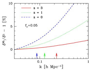
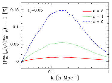
Appendix B Higher-order growth functions in a MDM model

In this appendix, we summarize the basic equations for higher-order growth functions in a MDM model defined in Sec II.3, which were used for the analysis presented in Sec. II.4.

Let us consider the second-order growth functions, $A^{(2)}_{\delta}$ and $B^{(2)}_{\delta}$, defined in Eq.(26). From the perturbation equation for second-order quantity $\delta_{\rm cb}^{(2)}$ (see Eq.(25)), the governing equations for $A^{(2)}_{\delta}$ and $B^{(2)}_{\delta}$ are obtained, and we have

$$\ddot{A}^{(2)}_{\delta}(k_{1},k_{2};t)+2H\,\dot{A}^{(2)}_{\delta}(k_{1},k_{2};t)-\frac{3}{2}H^{2}(1-\Omega_{w})\,f_{\rm cb}\,A^{(2)}_{\delta}(k_{1},k_{2};t)$$

$$\quad\quad\quad\quad\quad\quad\quad\quad\quad=\left[H\,\frac{dD_{\rm cb}(k_{1};t)}{d\ln a}D_{\rm cb}(k_{2};t)\right]^{.}+2H^{2}\,\frac{dD_{\rm cb}(k_{1};t)}{d\ln a}D_{\rm cb}(k_{2};t),$$ (50)

$$\ddot{B}^{(2)}_{\delta}(k_{1},k_{2};t)+2H\,\dot{B}^{(2)}_{\delta}(k_{1},k_{2};t)-\frac{3}{2}H^{2}(1-\Omega_{w})\,f_{\rm cb}\,B^{(2)}_{\delta}(k_{1},k_{2};t)$$

$$\quad\quad\quad\quad\quad\quad\quad\quad\quad=\frac{1}{2}\,H^{2}\,\frac{dD_{\rm cb}(k_{1};t)}{d\ln a}\frac{dD_{\rm cb}(k_{2};t)}{d\ln a}.$$ (51)

Note that in numerically solving the above equations, we retrieve only the inhomogeneous part of solutions so that the solution consistently approaches zero when going back to an initial time $t\to 0$. This treatment just corresponds to picking up the growing-mode solution consistently, since the source terms of the evolution equations involve the growing-mode solution of linear perturbations.

Next write down the governing equations for third-order growth functions defined in Eq.(27), $\mathcal{I}^{(3)}_{\delta}(k_{1},k_{2},k_{3})\,(\mathcal{I}=A,B,C,D,E,F)$, shortly abbreviated as $\mathcal{I}^{(3)}_{\delta}$. To do this, we first derive the perturbation equation for third-order quantity $\delta_{\rm cb}^{(3)}$. From Eq.(8), substitution of the linear and second-order solutions $\delta_{\rm cb}^{(1,2)}$ and $\theta_{\rm cb}^{(1,2)}$ leads to

$$\ddot{\delta_{\rm cb}}^{(3)}+2H\dot{\delta_{\rm cb}}^{(3)}-\frac{3}{2}H^{2}(1-\Omega_{w})\,f_{\rm cb}\delta_{\rm cb}^{(3)}$$

$$=\int\frac{d^{3}\mbox{\boldmath$k$}_{1}d^{3}\mbox{\boldmath$k$}_{2}d^{3}\mbox{\boldmath$k$}_{3}}{(2\pi)^{6}}\,\,\delta_{D}(\mbox{\boldmath$k$}-\mbox{\boldmath$k$}_{1}-\mbox{\boldmath$k$}_{2}-\mbox{\boldmath$k$}_{3})\hat{\Delta}(\mbox{\boldmath$k$}_{1})\hat{\Delta}(\mbox{\boldmath$k$}_{2})\hat{\Delta}(\mbox{\boldmath$k$}_{3})$$

$$\quad\quad\times\,\,\Bigl{[}\,\alpha_{1,23}\left\{\alpha_{2,3}\,\mathcal{S}^{A}_{1,2,3}(t)+\beta_{2,3}\,\mathcal{S}^{B}_{1,2,3}(t)\right\}-\alpha_{23,1}\left\{\alpha_{2,3}\,\mathcal{S}^{C}_{1,2,3}(t)+\beta_{2,3}\,\mathcal{S}^{D}_{1,2,3}(t)\right\}\Bigr{.}$$

$$\quad\quad\quad\quad\quad\quad\quad\quad\quad\quad\quad\quad\quad\quad\quad\Bigl{.}-\beta_{1,23}\,\left\{\alpha_{2,3}\,\mathcal{S}^{E}_{1,2,3}(t)+\beta_{2,3}\,\mathcal{S}^{F}_{1,2,3}(t)\right\}\Bigr{]},$$ (52)

where the quantities, $\alpha_{1,23}$, $\alpha_{23,1}$ and $\beta_{1,23}$ respectively indicate $\alpha(\mbox{\boldmath$k$}_{1},\mbox{\boldmath$k$}_{2}+\mbox{\boldmath$k$}_{3})$, $\alpha(\mbox{\boldmath$k$}_{2}+\mbox{\boldmath$k$}_{3},\mbox{\boldmath$k$}_{1})$ and $\beta(\mbox{\boldmath$k$}_{1},\mbox{\boldmath$k$}_{2}+\mbox{\boldmath$k$}_{3})$. Then, comparing the formal solution (27) with the above equation, we obtain the evolution equations for the third-order growth functions ${\mathcal{I}}^{(3)}_{\delta}$:

$$\ddot{\mathcal{I}}^{(3)}_{\delta 1,2,3}+2H\dot{\mathcal{I}}^{(3)}_{\delta 1,2,3}-\frac{3}{2}H^{2}(1-\Omega_{w})f_{\rm cb}\mathcal{I}^{(3)}_{\delta 1,2,3}=\mathcal{S}^{\mathcal{I}}_{1,2,3}.$$ (53)

Again, the above equations must be solved just retrieving the inhomogeneous part of the solution. Here, the source functions, $\mathcal{S}^{\mathcal{I}}_{1,2,3},\ (\mathcal{I}=A,B,C,D,E,F)$, are the scale- and time-dependent functions consisting of the linear and second-order growth functions. They are given by

$$\mathcal{S}^{A}_{1,2,3}(t) = \left[H\frac{dD_{\rm cb}(k_{1};t)}{d\ln a}A^{(2)}_{\delta}(k_{2},k_{3};t)\right]^{.}+2H^{2}\frac{dD_{\rm cb}(k_{1};t)}{d\ln a}A^{(2)}_{\delta}(k_{2},k_{3};t),$$

$$\mathcal{S}^{B}_{1,2,3}(t) = \left[H\frac{dD_{\rm cb}(k_{1};t)}{d\ln a}B^{(2)}_{\delta}(k_{2},k_{3};t)\right]^{.}+2H^{2}\frac{dD_{\rm cb}(k_{1};t)}{d\ln a}B^{(2)}_{\delta}(k_{2},k_{3};t),$$

$$\mathcal{S}^{C}_{1,2,3}(t) = \left[HD_{\rm cb}(k_{1};t)A^{(2)}_{\theta}(k_{2},k_{3};t)\right]^{.}+2H^{2}D_{\rm cb}(k_{1};t)A^{(2)}_{\theta}(k_{2},k_{3};t),$$

$$\mathcal{S}^{D}_{1,2,3}(t) = \left[HD_{\rm cb}(k_{1};t)B^{(2)}_{\theta}(k_{2},k_{3};t)\right]^{.}+2H^{2}D_{\rm cb}(k_{1};t)B^{(2)}_{\theta}(k_{2},k_{3};t),$$

$$\mathcal{S}^{E}_{1,2,3}(t) = H^{2}\frac{dD_{\rm cb}(k_{1};t)}{d\ln a}A^{(2)}_{\theta}(k_{2},k_{3};t),$$

$$\mathcal{S}^{F}_{1,2,3}(t) = H^{2}\frac{dD_{\rm cb}(k_{1};t)}{d\ln a}B^{(2)}_{\theta}(k_{2},k_{3};t),$$ (54)

In the above, the functions $A^{(2)}_{\theta}$ and $B^{(2)}_{\theta}$ are the second-order growth functions which appear in the solution of second-order velocity divergence $\theta^{(2)}_{\rm cb}$. These functions are related to the functions $A^{(2)}_{\delta}$ and $B^{(2)}_{\delta}$ through

$$A^{(2)}_{\theta}(k_{1},k_{2};t)=\frac{dD_{\rm cb}(k_{1};t)}{d\ln a}D_{\rm cb}(k_{2};t)-H^{-1}\dot{A}^{(2)}_{\delta}(k_{1},k_{2};t),\quad B^{(2)}_{\theta}(k_{1},k_{2};t)=-H^{-1}\dot{B}^{(2)}_{\delta}(k_{1},k_{2};t).$$ (55)

Finally, we note that in the limit of $f_{\rm cb}\to 1$ (i.e., case of massless neutrinos), there exist no free-streaming scales, and the linear growth function $D_{\rm cb}$ becomes independent of scales. From Eqs.(50), (51) and (53), this readily implies that all the second- and third-order growth functions become scale-independent. Then, employing the Einstein-de Sitter approximation, the analytical expressions for higher-order growth functions can be systematically obtained. In the Einstein-de Sitter approximation, all the calculations done in the Einstein-de Sitter universe are extended to apply to the other cosmological model by simply replacing the linear growth function in the Einstein-de Sitter universe with the one in the underlying cosmology. The detailed discussion on the validity of the Einstein-de Sitter approximation is given in  Bernardeau:1993qu ; Takahashi:2008yk ; Hiramatsu .

As a result, higher-order growth functions in the $f_{\rm cb}\to 1$ limit are analytically expressed as

$$A^{(2)}_{\delta}\to\frac{5}{7}D_{1}(t)^{2},\quad\quad B^{(2)}_{\delta}\to\frac{1}{7}D_{1}(t)^{2}.$$ (56)

for the second-order growth functions, and

$$\left\{A_{\delta}^{(3)},B_{\delta}^{(3)},C_{\delta}^{(3)},D_{\delta}^{(3)},E_{\delta}^{(3)},F_{\delta}^{(3)}\right\}\to\left\{\frac{5}{18},\frac{1}{18},-\frac{1}{6},-\frac{1}{9},-\frac{1}{21},-\frac{2}{63}\right\}\,D_{1}(t)^{3}.$$ (57)

for the third-order growth functions. For reference, in Fig. 11 we show nonlinear growth functions as in Fig. 1.

Figure 11: The 2nd-order and 3rd-order growth functions. The ratios of 2nd-order growth functions to the square of linear-oder growth functions, $A^{(2)}_{\delta}(k_{1},k_{2})/(D_{\rm cb}(k_{1})D_{\rm cb}(k_{2})$ (top left) and $B^{(2)}_{\delta}(k_{1},k_{2})/(D_{\rm cb}(k_{1})D_{\rm cb}(k_{2})$ (top right) are plotted (blue curved surfaces). In the case of the 3rd-order growth functions, the ratios to the cubed linear-oder growth functions, $\mathcal{I}^{(3)}_{\delta}/(D_{\rm cb}(k_{1})^{2}D_{\rm cb}(k_{2})),\ (\mathcal{I}=A-F)$ are shown (blue curved surfaces). Although the 3rd-order growth functions, $\mathcal{I}^{(3)}_{\delta}$ depend on three specific wavenumbers, it is sufficient to specify two wavenumbers to calculate $P^{(13)}_{\rm cb}(k)$. That is why we show the ratios such as the combination of $k_{1}$ and $k_{2}$, $\mathcal{I}^{(3)}_{\delta}(k_{1},k_{2},k_{1})$ and $\mathcal{I}^{(3)}_{\delta}(k_{1},k_{1},k_{2})$. Note that $\mathcal{I}^{(3)}_{\delta}(k_{1},k_{2},k_{1})=\mathcal{I}^{(3)}_{\delta}(k_{1},k_{1},k_{2})$ for $\mathcal{I}=B,D$ and $F$. For the reference, the constant values (red plane for 2nd-order and green plane for 3rd-order) are also shown. These constant values corresponds to the SPT treatment in a CDM model.

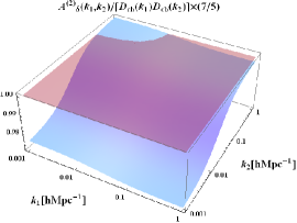
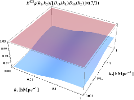
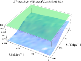
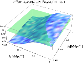
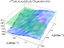
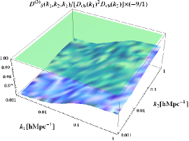
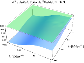
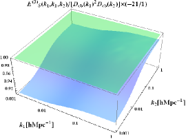
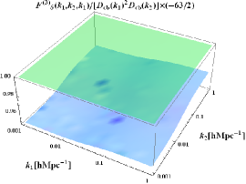
Appendix C Reparametrization of biasing parameters

In this appendix, we review the reparametrized biasing parameters proposed by Ref. McDonald:2006mx . In this treatment, the galaxy power spectrum can be consistently related to the matter power spectrum calculated from SPT.

The starting point is that the fluctuation of galaxies is expanded in Taylor series assuming the local biasing prescription. In the local biasing scheme, the galaxy density field at a given position is described as the local function of matter fluctuation at the same position. In Fourier space, the galaxy density field is described as

$$\delta_{g}(\mbox{\boldmath$k$}) = c_{1}\delta_{\rm m}(\mbox{\boldmath$k$})+\frac{c_{2}}{2}\int\frac{d^{3}\mbox{\boldmath$q$}}{(2\pi)^{3}}~{}\delta_{\rm m}(\mbox{\boldmath$q$})\delta_{\rm m}(\mbox{\boldmath$k$}-\mbox{\boldmath$q$})$$ (58)

$$+\frac{c_{3}}{6}\int\frac{d^{3}\mbox{\boldmath$q$}_{1}d^{3}\mbox{\boldmath$q$}_{2}}{(2\pi)^{6}}~{}\delta_{\rm m}(\mbox{\boldmath$q$}_{1})\delta_{\rm m}(\mbox{\boldmath$q$}_{2})\delta_{\rm m}(\mbox{\boldmath$k$}-\mbox{\boldmath$q$}_{1}-\mbox{\boldmath$q$}_{2})+\epsilon(\mbox{\boldmath$k$})+\mathcal{O}({\delta^{(1)}_{\rm m}}^{4}),$$

where the $c_{i}$’s are the biasing parameters. The quantity $\epsilon$ represents the residual random field which cannot be represented by the matter fluctuations. We assume that randomness of $\epsilon$ is described by a white noise, and is uncorrelated with $\delta_{\rm m}$, i.e., $\langle\epsilon^{2}\rangle=N_{0}$ and $\langle\epsilon\delta_{\rm m}\rangle=0$. Then, the galaxy density power spectrum $P_{\rm g}$ up to the one-loop level is calculated as

$$P_{\rm g} = c_{1}^{2}P^{\rm NL}_{\rm m}(k)+\left(c_{1}c_{3}\sigma^{2}+\frac{68}{21}c_{1}c_{2}\sigma^{2}\right)P^{\rm L}_{\rm m}(k)$$ (59)

$$+2c_{1}c_{2}\int\frac{d^{3}\mbox{\boldmath$q$}}{(2\pi)^{3}}~{}P^{\rm L}_{\rm m}(q)P^{\rm L}_{\rm m}(|\mbox{\boldmath$k$}-\mbox{\boldmath$q$}|){\cal F}^{(2)}_{\delta}(\mbox{\boldmath$q$},\mbox{\boldmath$k$}-\mbox{\boldmath$q$})$$

$$+\frac{c^{2}_{2}}{2}\int\frac{d^{3}\mbox{\boldmath$q$}}{(2\pi)^{3}}~{}P^{\rm L}_{\rm m}(q)P^{\rm L}_{\rm m}(|\mbox{\boldmath$k$}-\mbox{\boldmath$q$}|)+N_{0},$$

where the constant parameter $\sigma^{2}$ is defined as $\sigma^{2}\equiv\int d^{3}\mbox{\boldmath$q$}~{}P^{\rm L}_{\rm m}(q)/(2\pi)^{3}$, and the function $\mathcal{F}^{(2)}_{\delta}(\mbox{\boldmath$k$},\mbox{\boldmath$k$}^{\prime})$ is the Fourier kernel of the second-order density perturbation:

$$\mathcal{F}^{(2)}_{\delta}(\mbox{\boldmath$k$},\mbox{\boldmath$k$}^{\prime})\equiv\frac{5}{7}+\frac{1}{2}\frac{\mbox{\boldmath$k$}\cdot\mbox{\boldmath$k$}^{\prime}}{\mbox{\boldmath$k$}\mbox{\boldmath$k$}^{\prime}}\left(\frac{k^{\prime}}{k}+\frac{k}{k^{\prime}}\right)+\frac{2}{7}\left(\frac{\mbox{\boldmath$k$}\cdot\mbox{\boldmath$k$}^{\prime}}{kk^{\prime}}\right)^{2}.$$ (60)

While the calculation in the above is exact up to the fourth-order in density, due to the truncation at finite order, the expression (59) suffers from several unphysical behaviors such as an apparent divergence and anomalous low-$k$ power Heavens:1998es . To remedy this, Ref. McDonald:2006mx proposed a way to regularize the expression (59) by reorganizing several terms and reparametrizing the biasing parameters. In this treatment, the first line of Eq.(59) is rewritten as

$$c_{1}^{2}P^{\rm NL}_{\rm m}(k)+\left(c_{1}c_{3}\sigma^{2}+\frac{68}{21}c_{1}c_{2}\sigma^{2}\right)P^{\rm L}_{\rm m}(k)\to b_{1}^{2}P^{\rm NL}_{\rm m}(k)\equiv\left[c_{1}^{2}+c_{1}c_{3}\sigma^{2}+\frac{68}{21}c_{1}c_{2}\sigma^{2}\right]P^{\rm NL}_{\rm m}(k).$$ (61)

Further, the apparent divergence arising from the third line is absorbed by redefining the parameter $N_{0}$ as

$$N\equiv N_{0}+\frac{c_{2}^{2}}{2}\int\frac{d^{3}\mbox{\boldmath$q$}}{(2\pi)^{3}}~{}P^{\rm L}_{\rm m}(q)^{2}.$$ (62)

Then, the galaxy power spectrum is re-expressed as follows:

$$P_{\rm g}(k) = b_{1}^{2}\left[P^{\rm NL}_{\rm m}(k)+b_{2}P_{\rm b2,\delta}(k)+b_{2}^{2}P_{\rm b22}(k)\right]+N,$$ (63)

$$P_{\rm b2,\delta}(k) \equiv 2\int\frac{d^{3}\mbox{\boldmath$q$}}{(2\pi)^{3}}~{}P^{\rm L}_{\rm m}(q)P^{\rm L}_{\rm m}(|\mbox{\boldmath$k$}-\mbox{\boldmath$q$}|)\mathcal{F}^{(2)}_{\delta}(\mbox{\boldmath$q$},\mbox{\boldmath$k$}-\mbox{\boldmath$q$}),$$ (64)

$$P_{\rm b22}(k) \equiv \frac{1}{2}\int\frac{d^{3}\mbox{\boldmath$q$}}{(2\pi)^{3}}~{}P^{\rm L}_{\rm m}(q)[P^{\rm L}_{\rm m}(|\mbox{\boldmath$k$}-\mbox{\boldmath$q$}|)-P^{\rm L}_{\rm m}(q)].$$ (65)

As a result, the galaxy power spectrum in the weakly nonlinear regime can be described with the only three parameters, $b_{1},b_{2}$ and $N$. Recently, the validity of the expression (65) has been examined in some details in Ref. Jeong:2008rj . They reported that this reparametrization scheme can fit well to the power spectrum of halos and galaxies in millennium simulations, and the cosmological parameters can be correctly estimated using Eq.(65) as a template in an unbiased fashion.

Appendix D Nonlinear bias parameters based on halo-model

We here summarize how to determine the fiducial values of the biasing parameters $b_{1}$, $b_{2}$ and $N$ listed in Table 1, which are used in the Fisher matrix analysis in Sec. V.3.

Following the treatment in Refs. Seo:2003pu ; Takada:2005si , we determine the linear biasing parameter $b_{1}$ at a given redshift so that the condition $\sigma_{8,\rm g}(z)=1$ is satisfied, where we define

$$\sigma_{8,\rm g}(z)=b_{1}(z)\sigma_{8,\rm m}(z)\sqrt{1+\frac{2F_{\rm m}(z)}{3}+\frac{F_{\rm m}(z)^{2}}{5}},$$ (66)

with $F_{\rm m}(z)=-d\ln D_{1}(z)/d\ln(1+z)$. The function $D_{1}(z)$ is the linear growth rate for $\Lambda$CDM model, which we compute from the fiducial cosmological parameters just setting $f_{\nu}=0$. For SDSS LRG and BOSS surveys, their target samples are LRGs whose clustering properties are relatively known from the observations, and the linear biasing parameter is measured as $b_{1}\sim 2.10$ at $z=0.3$. Hence, when considering these surveys, we simply adopt this value, and the linear biasing parameters at different redshifts are determined from (66) just rescaling the condition $\sigma_{8,\rm g}(z)=1$ to $\sigma_{8,\rm g}(z)=\sigma_{8,\rm g}(0.3)$ with $b_{1}(0.3)=2.10$.

The non-linear biasing parameter $b_{2}$ in the expression (65) is related to the original parameters $c_{i}$ in Eq.(58) as

$$b_{2}=\frac{c_{2}}{c_{1}}.$$ (67)

The biasing parameters $c_{1}$ and $c_{2}$ can be estimated from the halo-model approach (e.g., Scoccimarro:2000gm ). According to this prescription, we obtain

$$c_{i}=\frac{1}{\bar{n}_{\rm g}}\int_{M_{\rm min}}^{\infty}dM~{}n_{\rm h}(M,z)b^{\rm h}_{i}(M,z)\langle N\rangle_{M},$$ (68)

where the function $n_{\rm h}(M,z)$ is the halo mass function for the given mass $M$ and redshift $z$, and the quantity $b^{h}_{i}(M,z)$ is the halo biasing parameter. The expectation value $\langle N\rangle_{M}$ is the so-called halo-occupation distribution, which describes the mean number of galaxies per halo with mass $M$. We here set $\langle N\rangle_{M}=1$ for simplicity. We adopt the Sheth and Tormen formula for mass function $n_{\rm h}(M,z)$ Sheth:1999mn :

$$n_{\rm h}(M,z)=-\frac{\bar{\rho}_{\rm m0}}{M^{2}}\frac{d\ln\sigma}{d\ln M}f(\nu)\,\,;\quad f(\nu)=A\sqrt{\frac{2q}{\pi}}[1+(q\nu^{2})^{-p}]\nu e^{-q\nu^{2}/2},$$ (69)

with $A=0.322$, $p=0.3$, and $q=0.707$. The density threshold $\nu$ is set to $\delta_{c}/\sigma(M,z)$ with $\delta_{c}=1.686$. Then, the halo biasing parameters $b^{\rm h}_{i}$ can be calculated from Eq.(69) as

$$b^{\rm h}_{1}(M,z) = 1+\epsilon_{1}+E_{1},$$ (70)

$$b^{\rm h}_{2}(M,z) = \frac{8}{21}(\epsilon_{1}+E_{1})+\epsilon_{2}+E_{2},$$ (71)

where we define

$$\epsilon_{1}=\frac{q\nu^{2}-1}{\delta_{c}},\quad\epsilon_{2}=\frac{q\nu^{2}}{\delta_{c}}\frac{q\nu^{2}-3}{\delta_{c}},$$ (72)

$$E_{1}=\frac{2p}{\delta_{c}}\frac{1}{1+(q\nu^{2})^{p}},\quad\frac{E_{2}}{E_{1}}=\frac{1+2p}{\delta_{c}}+2\epsilon_{1}.$$ (73)

In the expression (68), there appears the minimum halo mass, $M_{\rm min}$, which can be determined from the condition,

$$\overline{n}_{\rm g}=\int_{M_{\rm min}}dM~{}n_{h}(M,z)\langle N\rangle_{M}.$$ (74)

Finally, it seems rather difficult to determine the fiducial value of the remaining parameter $N$, because physical meaning of the parameter $N$ is less clear. In this paper, we just adopt the relation (62), and compute $N$ assuming $N_{0}=0$:

$$N=\frac{{c^{\rm h}_{2}}^{2}}{2}\int\frac{d^{3}{\bf q}}{(2\pi)^{3}}P^{\rm L}_{\rm m}(q)^{2}.$$ (75)

Appendix E Systematic bias for the best-fit parameters

In this appendix, we briefly review how to estimate the biases in best-fit parameters arising from the systematic effects. We are especially concerned with the impact of neglecting massive neutrinos on the dark energy constraints. In this case, the biased parameter estimation is obtained by fitting the observational data to the power spectrum template incorrectly assuming $f_{\nu}=0$. Let us write down the observed power spectrum as

$$P^{\rm obs}_{\rm g}(k) = P^{f_{\nu}\neq 0}_{\rm g}(k)+P^{\rm noise}_{\rm g}(k)$$ (76)

$$= P^{f_{\nu}=0}_{\rm g}(k)+P^{\rm sys}_{\rm g}(k)+P^{\rm noise}_{\rm g}(k),$$

where $P^{\rm noise}_{\rm g}(k)$ denotes the instrumental noise, while the systematics in power spectrum, $P^{\rm sys}_{\rm g}(k)$ is defined as $P^{\rm sys}_{\rm g}(k)\equiv P^{f_{\nu}\neq 0}_{\rm g}(k)-P^{f_{\nu}=0}_{\rm g}(k)$. Then, the systematic bias in a certain parameter $\delta p_{\alpha}$ is computed in (e.g., Joachimi:2009fr ) as

$$\delta p_{\alpha}=\sum_{\beta}({\bf F}^{-1})_{\alpha\beta}S_{\beta},$$ (77)

where ${\bf F}$ is the full Fisher matrix (namely, ${\bf F}_{\alpha\beta}={\bf F}_{\alpha\beta}^{\rm galaxy}+{\bf F}_{\alpha\beta}^{\rm CMB}$) in which the neutrino parameter $f_{\nu}$ is excluded from the matrix element. Note that in computing ${\bf F}$, the fiducial parameter for $f_{\nu}$ must be set to $f_{\nu}=0$, because we consider the situation that the observed power spectrum is incorrectly fitted to the template neglecting massive neutrinos. Here, the vector quantity $S_{\alpha}$ is represented as $S_{\alpha}=S^{\rm CMB}_{\alpha}+S^{\rm galaxy}_{\alpha}$, which are respectively given by

$$S^{\rm CMB}_{\alpha} = \sum_{\ell}\sum_{X,Y}C^{X,{\rm sys}}_{\ell}\{\Xi(\hat{C}^{X}_{\ell},\hat{C}^{Y}_{\ell})\}^{-1}\frac{\partial C^{Y}_{\ell}}{\partial p_{\alpha}},$$ (78)

$$S^{\rm galaxy}_{\alpha} = \sum_{i}\frac{V_{\rm s}(z_{i})}{4\pi^{2}}\int^{k_{\rm max}(z_{i})}_{k_{\rm min}}k^{2}dk~{}\frac{P^{\rm est,sys}_{\rm g}(k;z_{i})}{P^{\rm est}_{\rm g}(k;z_{i})}\frac{\partial\ln P^{\rm est}_{\rm g}(k;z_{i})}{\partial p_{\alpha}}\left[\frac{\bar{n}_{\rm g}(z_{i})P^{\rm est}_{\rm g}(k;z_{i})}{\bar{n}_{\rm g}(z_{i})P^{\rm est}_{\rm g}(k;z_{i})+1}\right]^{2},$$ (79)

where the angular power spectrum for CMB, $C^{X,{\rm sys}}_{\ell}$, is defined similarly to the case of galaxy power spectrum, i.e., $C^{X,{\rm sys}}_{\ell}\equiv C^{X,f_{\nu}\neq 0}-C^{X,f_{\nu}=0}$. Note again that we set $f_{\nu}=0$ in computing $C^{X}_{\ell}$ and $P^{\rm est}_{\rm g}$.

References

- (1) E. Komatsu et al., arXiv:0803.0547 [astro-ph].
- (2) S. Dodelson, Modern Cosmology, Academic Press, San Diego (2003).
- (3) S. Fukuda et al. [Super-Kamiokande Collaboration], Phys. Rev. Lett. 85, 3999 (2000).
- (4) S. N. Ahmed et al. [SNO Collaboration], Phys. Rev. Lett. 92, 181301 (2004).
- (5) K. Eguchi et al. [KamLAND Collaboration], Phys. Rev. Lett. 90, 021802 (2003).
- (6) T. Arakki et al. [KamLAND Collaboration], Phys. Rev. Lett. 94 081801 (2005).
- (7) R. D. McKeown and P. Vogel, Phys. Rept. 394, 315 (2004).
- (8) B. Kayser, arXiv:hep-ph/0506165.
- (9) J. Bonn et al., Nucl.Phys.B (Proc. Suppl.) 91, 273 (2001).
- (10) K. Ichikawa, M. Fukugita and M. Kawasaki, Phys. Rev. D 71, 043001 (2005).
- (11) M. Fukugita, K. Ichikawa, M. Kawasaki and O. Lahav, Phys. Rev. D 74, 027302 (2006).
- (12) M. Kowalski et al., Astrophys. J. 686, 749 (2008).
- (13) D. J. Eisenstein et al., Astrophys. J. 633, 560 (2005); W. J. Percival et al., Astrophys. J. 657, 51 (2007); W. J. Percival et al., Mon. Not. Roy. Astron. Soc. 381, 1053 (2007); E. Gaztanaga, A. Cabre and L. Hui, arXiv:0807.3551 [astro-ph]; W. J. Percival et al., arXiv:0907.1660 [astro-ph.CO].
- (14) J. R. Bond, G. Efstathiou and J. Silk, Phys. Rev. Lett 45, 1980 (1980).
- (15) W. Hu, D. J. Eisenstein and M. Tegmark, Phys. Rev. Lett. 80, 5255 (1998).
- (16) Ø. Elgarøy et al., Phys. Rev. Lett 89, 061301 (2002).
- (17) M. Tegmark et al., Phys. Rev. D 74, 123507 (2006).
- (18) K. Ichiki, M. Takada and T. Takahashi, Phys. Rev. D 79, 023520 (2009).
- (19) T. D. Kitching et al., Phys. Rev. D 77, 103008 (2008).
- (20) U. Seljak, A. Slosar and P. McDonald, JCAP 0610, 014 (2006).
- (21) J. R. Pritchard and E. Pierpaoli, Phys. Rev. D 78, 065009 (2008).
- (22) M. Sumiyoshi et al., arXiv:0902.2064 [astro-ph.CO].
- (23) M. Takada, E. Komatsu and T. Futamase, Phys. Rev. D 73, 083520 (2006).
- (24) S. Hannestad and Y. Y. Y. Wong, JCAP 0707, 004 (2007).
- (25) F. B. Abdalla and S. Rawlings, Mon. Not. R. Astron. Soc. 381, 1313 (2007).
- (26) D. Jeong and E. Komatsu, Astrophys. J. 651, 619 (2006).
- (27) R. Angulo, C. M. Baugh, C. S. Frenk and C. G. Lacey, Mon. Not. Roy. Astron. Soc. 383, 755 (2008).
- (28) R. Takahashi et al., Mon. Not. Roy. Astron. Soc. 389, 1675 (2008).
- (29) A. G. Sanchez, C. M. Baugh and R. Angulo, arXiv:0804.0233 [astro-ph].
- (30) H. J. Seo, E. R. Siegel, D. J. Eisenstein and M. White, arXiv:0805.0117 [astro-ph].
- (31) D. Jeong and E. Komatsu, arXiv:0805.2632 [astro-ph].
- (32) T. Nishimichi et al., arXiv:0810.0813 [astro-ph].
- (33) P. McDonald, Phys. Rev. D 75, 043514 (2007).
- (34) P. Valageas, Astron. Astrophys. 465, 725 (2007).
- (35) S. Matarrese and M. Pietroni, JCAP 0706, 026 (2007).
- (36) T. Nishimichi et al., Publ. Astron. Soc. Jap. 59, 1049 (2007).
- (37) M. Crocce and R. Scoccimarro, arXiv:0704.2783 [astro-ph].
- (38) T. Matsubara, Phys. Rev. D 77, 063530 (2008).
- (39) A. Taruya and T. Hiramatsu, Astrophys. J. 674, 617 (2008).
- (40) M. Pietroni, arXiv:0806.0971 [astro-ph].
- (41) H. Nomura, K. Yamamoto and T. Nishimichi, JCAP 0810 031 (2008).
- (42) J. Carlson, M. White and N. Padmanabhan, arXiv:0905.0479 [astro-ph.CO].
- (43) A. Taruya, T. Nishimichi, S. Saito and T. Hiramatsu, arXiv:0906.0507 [astro-ph.CO].
- (44) J. Lesgourgues and S. Pastor, Phys. Rept. 429, 307 (2006).
- (45) F. Bernardeau, S. Colombi, E. Gaztanaga and R. Scoccimarro, Phys. Rept. 367, 1 (2002).
- (46) S. Saito, M. Takada and A. Taruya, Phys. Rev. Lett. 100, 191301 (2008).
- (47) P. McDonald, Phys. Rev. D 74, 103512 (2006).
- (48) M. Tegmark et al., Astrophys. J. 606, 702 (2004).
- (49) A. Taruya, Astrophys. J. , 537, 37 (2000).
- (50) S. Pueblas and R. Scoccimarro, arXiv:0809.4606 [astro-ph].
- (51) C. P. Ma and E. Bertschinger, Astrophys. J. 455, 7 (1995).
- (52) U. Seljak and M. Zaldarriaga, ApJ, 1996, 469, 437
- (53) A. Lewis, A. Challinor and A. Lasenby, Astrophys. J. 538, 473 (2000).
- (54) D. J. Eisenstein and W. Hu, Astrophys. J. 511, 5 (1999).
- (55) W. Hu and D. J. Eisenstein, Astrophys. J. 498, 497 (1998).
- (56) F. Bernardeau, Astrophys. J. 433, 1 (1994).
- (57) R. Takahashi, arXiv:0806.1437 [astro-ph].
- (58) T. Hiramatsu and A. Taruya, Phys. Rev. D 79, 103526 (2009).
- (59) N. Makino, M. Sasaki, and Y. Suto, Phys. Rev. D 46, 585 (1992).
- (60) B. Jain and E. Bertschinger, Astrophys. J. 431, 495 (1994).
- (61) Y. Y. Y. Wong, JCAP 0810, 035 (2008).
- (62) A. Kiakotou, O. Elgaroy and O. Lahav, Phys. Rev. D 77, 063005 (2008).
- (63) R. E. Smith et al. [The Virgo Consortium Collaboration], Mon. Not. Roy. Astron. Soc. 341, 1311 (2003).
- (64) J. Brandbyge, S. Hannestad, T. Haugboelle and B. Thomsen, JCAP 0808, 020 (2008).
- (65) J. Brandbyge and S. Hannestad, arXiv:0812.3149 [astro-ph].
- (66) R. Takahashi et al., Astrophys. J. 700, 479 (2009).
- (67) J. N. Fry and E. Gaztanaga, Astrophys. J. 425, 1 (1994).
- (68) J. N. Fry, Astrophys. J. 461, L65 (1996).
- (69) M. Tegmark and P. J. E. Peebles, Astrophys. J. 500, L79 (1998)
- (70) L. Hui and K. P. Parfrey, Phys. Rev. D 77, 043527 (2008).
- (71) A. F. Heavens, S. Matarrese and L. Verde, Mon. Not. Roy. Astron. Soc. 301, 797 (1998).
- (72) U. Seljak, Mon. Not. Roy. Astron. Soc. 318, 203 (2000)
- (73) R. E. Smith, R. Scoccimarro and R. K. Sheth, Phys. Rev. D 75, 063512 (2007)
- (74) C. Alcock and B. Paczynski, Nature, 281, 358 (1979).
- (75) H. J. Seo and D. J. Eisenstein, Astrophys. J. 598, 720 (2003).
- (76) T. Matsubara and A. S. Szalay, Phys. Rev. Lett. 90, 021302 (2003).
- (77) L. Perotto, J. Lesgourgues, S. Hannestad, H. Tu and Y. Y. Y. Wong, JCAP 0610, 013 (2006).
- (78) M. Tegmark, Phys. Rev. Lett. 79, 3806 (1997).
- (79) A. Klypin, J. Holtzman, J. Primack and E. Regos, Astrophys. J. 416, 1 (1993).
- (80) M. Takada and B. Jain, arXiv:0810.4170 [astro-ph].
- (81) E. Sefusatti, M. Crocce, S. Pueblas and R. Scoccimarro, Phys. Rev. D 74, 3522 (2007).
- (82) [Planck Collaboration], arXiv:astro-ph/0604069.
- (83) T. Matsubara, Astrophys. J. , 615, 573 (2004).
- (84) N. Kaiser, Astrophys. J. 284, L9 (1984).
- (85) A. J. Albrecht et al., arXiv:astro-ph/0609591.
- (86) J. Lesgourgues, S. Matarrese, M. Pietroni and A. Riotto, JCAP 0906, 017 (2009).
- (87) A. Lewis and A. Challinor, Phys. Rept. 429, 1 (2006).
- (88) D. Munshi, P. Valageas, L. Van Waerbeke and A. Heavens, Phys. Rept. 462, 67 (2008).
- (89) S. Singh and C. P. Ma, Phys. Rev. D 67, 023506 (2003).
- (90) A. Ringwald and Y. Y. Y. Wong, JCAP 0412, 005 (2004).
- (91) K. Abazajian et al., Phys. Rev. D 71, 043507 (2005).
- (92) M. Shoji and E. Komatsu, arXiv:0903.2669 [astro-ph.CO].
- (93) R. Scoccimarro, R. K. Sheth, L. Hui and B. Jain, Astrophys. J. 546, 20 (2001).
- (94) R. K. Sheth and G. Tormen, Mon. Not. Roy. Astron. Soc. 308, 119 (1999).
- (95) B. Joachimi and P. Schneider, arXiv:0905.0393 [astro-ph.CO].
- (96) http://www.science.doe.gov/hep/hepap/feb2007/hepap_bennett_feb07.pdf.