On the Chaotic Flux Dynamics in a Long Josephson Junction

Abstract.

Flux dynamics in an annular long Josephson junction is studied. Three main topics are covered. The first is chaotic flux dynamics and its prediction via Melnikov integrals. It turns out that DC current bias cannot induce chaotic flux dynamics, while AC current bias can. The existence of a common root to the Melnikov integrals is a necessary condition for the existence of chaotic flux dynamics. The second topic is on the components of the global attractor and the bifurcation in the perturbation parameter measuring the strength of loss, bias and irregularity of the junction. The global attractor can contain co-existing local attractors e.g. a local chaotic attractor and a local regular attractor. In the infinite dimensional phase space setting, the bifurcation is very complicated. Chaotic attractors can appear and disappear in a random fashion. Three types of attractors (chaos, breather, spatially uniform and temporally periodic attractor) are identified. The third topic is ratchet effect. Ratchet effect can be achieved by a current bias field which corresponds to an asymmetric potential, in which case the flux dynamics is ever lasting chaotic. When the current bias field corresponds to a symmetric potential, the flux dynamics is often transiently chaotic, in which case the ratchet effect disappears after sufficiently long time.

1. Introduction

The recently developed theory [12] on chaos in partial differential equations has the greatest potential of significance in its abundant applications in science and engineering. The variety of the specific problems also stimulates innovation of the theory. In these representative publications [13] [14] [15] [17] [18] [19] [20] [21], two categories of the theory were developed. The category developed in [13] [14] [15] involves transversal homoclinic orbits, and a shadowing technique is used to prove the existence of chaos. This category is very complete. The category in [17] [18] [19] [20] [21] deals with Silnikov (non-transversal) homoclinic orbits, and a geometric construction of Smale horseshoes is employed. This category is not very complete. The main machineries for locating homoclinic orbits are (1). Darboux transformations, (2). Isospectral theory, (3). Persistence of invariant manifolds and Fenichel fibers, (4). Melnikov analysis and shooting technique. Overall, the two categories of the theory on chaos in partial differential equations can be regarded as a new development at the intersection among Integrable Theory, Dynamical System Theory, and Partial Differential Equations [12]. In this article, we will apply the above chaos theory to study the chaotic flux dynamics in a long Josephson junction.

A Josephson junction consists of three parts: two superconductors separated by a thin ($\sim 10$ Å) dielectric barrier. The main character of a Josephson junction is that it behaves as a single superconductor. In particular, electric flux called fluxons can travel through the dielectric barrier through Josephson tunneling. In general, the scenario is as follows: when two superconductors are separated by a macroscopic distance, their phases can change independently. As the two superconductors are moved closer to about $30$ Å separation, quasiparticles can flow from one superconductor to the other by means of single electron tunneling. When the separation is reduced to $10$ Å, Cooper pairs can flow from one superconductor to the other (Josephson tunneling). In this case, phase correlation is realized between the two superconductors, and the whole Josephson junction behaves as a single superconductor. This phenomenon was predicted by Brian Josephson in 1962 [9]. It has significant applications in quantum-mechanical circuits. The governing equations are [3]

$$V(t)=\frac{\hbar}{2e}\frac{du}{dt},\quad I(t)=I_{c}\sin u(t)$$

where $V(t)$ and $I(t)$ are the voltage and current across the Josephson junction, $u$ is the phase difference between the wave functions in the two superconductors, the constant $I_{c}$ is called the critical current, and the constant $\frac{\hbar}{2e}$ is the magnetic flux quantum. Interesting simple phenomena can be observed from the above governing equations, e.g. when $V(t)$ is constant $V_{0}$ in $t$, $u$ is linear in $t$, then the current $I(t)$ will be an AC current with amplitude $I_{c}$ and frequency $\frac{2e}{\hbar}V_{0}$. This shows that a Josephson junction can be a perfect voltage-to-frequency converter. Significant applications of a Josephson junction can be found in many areas, e.g. in medicine for measurement of small currents in the brain and the heart. Josephson junction may also provide key ingredients for future quantum computers. For more details on the physics of the Josephson junction, see [3].

When a Josephson junction has one or more dimensions longer than the rest, i.e. a long Josephson junction (LJJ), the phase difference $u$ is also a function of spatial coordinates along the longer dimensions. In this article, we will focus on one longer dimension case. It is well known that the flux dynamics in a long Josephson junction (LJJ) is described by the so-called perturbed sine-Gordon equation [3]

(1.1) $$u_{tt}=c^{2}u_{xx}+\sin u+\epsilon f$$

where again $u$ is the phase difference between the two superconductors, and $c$ is a constant. The above equation is the rescaled standard form. In dealing with real junctions, one must take into account losses, bias, and junction irregularities which influence the flux dynamics [3]. These effects are of perturbation nature, and accounted for by the term $\epsilon f$ where $\epsilon$ is the perturbation parameter. Different forms of $\epsilon f$ can even by set up in experiments. Typically $\epsilon f$ takes the following forms:

• $\epsilon f=-\epsilon\alpha u_{t}+\epsilon\gamma$, where $-\epsilon\alpha u_{t}$ represents shunt loss and $\epsilon\gamma$ represents DC current bias [3].

• $\epsilon f=-\epsilon\alpha u_{t}+\epsilon\beta u_{txx}+\epsilon\gamma$, where $\epsilon\beta u_{txx}$ represents longitudinal loss [3].

• $\epsilon f=-\epsilon\alpha u_{t}+\epsilon\gamma+\epsilon a\sin\omega t$, where $\epsilon a\sin\omega t$ represents AC current bias [2].

• $\epsilon f=-\epsilon\alpha u_{t}+\epsilon\gamma\cos x+\epsilon a\sin\omega t$, where $\epsilon\gamma\cos x$ represents AC current field [4] [24].

• $\epsilon f=-\epsilon\alpha u_{t}+\epsilon g(x)+\epsilon a\sin\omega t$, where $\epsilon g(x)$ represents spatially periodic current field [4].

Of course, many other forms of $\epsilon f$ can also be set up in experiments. There is an abundant literature on long Josephson junctions, for a sample, see [11, 1, 6, 26, 25, 23, 22, 10].

Travelling wave solutions of (1.1) satisfy an ordinary differential equation which had been studied numerically since as early as 1968 by Johnson [8] using an analog-digital computer, till most recently [5] via analytical and numerical tools.

In this article, we shall study the full partial differential equation. When $\epsilon=0$, equation (1.1) is the well-known sine-Gordon equation. Two well-known types of solutions to the sine-Gordon equation are the kink and breather solutions. The simplest kink solution is independent of the space variable $x$. Such a simple kink can be observed in experiemnts for Josephson junctions. As $t\rightarrow\pm\infty$, the kink $u(t)$ approaches e.g. $0$ and $2\pi$. In terms of the current and voltage ($I(t),V(t)$) mentioned above, this corresponds to a closed loop — named a vortex or a fluxon. In the infinite dimensional phase space setting of the current article, this simple kink also represents a heteroclinic orbit. A breather oscillates periodically in time (breathing) and decays in space ($x\rightarrow\pm\infty$). In our current setting, we switch the space and time, therefore, the breather is now spatially periodic and temporally homoclinic, i.e. a homoclinic orbit. For long Josephson junctions, spatial dependence is significant, dynamics beyond the simple kink becomes crucial. More sophisticated solutions incorporating both the kink and the breather have been constructed [16]. In the phase space, these represent heteroclinic orbits which depend on both time and space. Together, these heteroclinic orbits form a two-dimensional heteroclinic cycle. The current article will focus its study on the neighborhood of this heteroclinic cycle. Three main topics will be covered. The first is chaotic flux dynamics and its prediction via Melnikov integrals (sections 4,5,6). The second is on the components of the global attractor and the bifurcation in the perturbation parameter (section 7). The third is ratchet effect (section 8). Section 9 is the conclusion.

2. The Phase Space

We pose periodic boundary condition on the above perturbed sine-Gordon equation (1.1),

(2.1) $$u(t,x+2\pi)=u(t,x).$$

This boundary condition corresponds to an annular LJJ [24] [4]. Convenient for mathematical studies, a more restricted condition — the even constraint may be imposed

(2.2) $$u(t,-x)=u(t,x)$$

which corresponds to a mirror symmetry of the annular LJJ. We restrict the parameter $c$ to the interval $c\in(0.5,1)$ to minimize the number of unstable modes of $u=0$ to two. (1.1) is invariant under $u\rightarrow u+2\pi$. When $\epsilon=0$, it is also invariant under $u\rightarrow-u$. (1.1) is globally well-posed [15], i.e. for any $(u^{0},u^{0}_{t})\in H^{n+1}\times H^{n}$ (the Sobolev spaces on $[0,2\pi]$) where $n\geq 1$ is an integer, there exists a unique mild solution to (1.1), $(u(t),u_{t}(t))\in C([0,\infty),H^{n+1}\times H^{n})$, such that $(u(0),u_{t}(0))=(u^{0},u^{0}_{t})$. One can introduce the evolution operator $F^{t}$ as $(u(t),u_{t}(t))=F^{t}(u^{0},u^{0}_{t})$. For any fixed $t\in[0,\infty)$, $F^{t}$ is a $C^{\infty}$ map. The space $H^{n+1}\times H^{n}$ will be the phase space where the perturbed sine-Gordon flow (1.1) is defined.

3. Isospectral Integrable Theory

When $\epsilon=0$, the unstable manifolds of $u_{+}=0$ and $u_{-}=2\pi$, $W^{u}_{\pm}$ form a 2-dimensional heteroclinic cycle whose explicit expression can be obtained through Darboux transformations [16]:

(3.1) $$u_{1} = 2\arccos(\tanh\tau)$$

$$-4\arctan\bigg{[}\frac{\sigma(\pm\tanh\tau\ \mbox{sech}\ \hat{\tau}\cos x-\ \mbox{sech}\ \tau\tanh\hat{\tau})}{1-\sigma(\tanh\tau\tanh\hat{\tau}\pm\ \mbox{sech}\ \tau\ \mbox{sech}\ \hat{\tau}\cos x)}\bigg{]}\ ,$$

(3.2) $$u_{2} = 2\pi-2\arccos(\tanh\tau)$$

$$-4\arctan\bigg{[}\frac{\sigma(\pm\tanh\tau\ \mbox{sech}\ \hat{\tau}\cos x+\ \mbox{sech}\ \tau\tanh\hat{\tau})}{1-\sigma(\tanh\tau\tanh\hat{\tau}\mp\ \mbox{sech}\ \tau\ \mbox{sech}\ \hat{\tau}\cos x)}\bigg{]}\ ,$$

where the ranges of $\arccos$ and $\arctan$ are [$0,\pi$] and ($-\pi/2,\pi/2$), and ($\tau,\sigma,\hat{\tau}$) are given by

$$\tau=t-\rho,\ \sigma=\sqrt{1-c^{2}},\ \hat{\tau}=\sigma t-\hat{\rho}=\sigma\tau-\Delta\rho,\ \Delta\rho=\hat{\rho}-\sigma\rho,$$

and $\rho$ and $\hat{\rho}$ are two real parameters. This heteroclinic cycle satisfies both the periodic boundary condition and the even constraint (2.1) and (2.2). A topological illustration of the heteroclinic cycle is shown in Figure 1. The heteroclinic cycle incorporates both kink and breather characteristics. The homoclinic degeneracy to be discussed later corresponds to the breather characteristic (when time and space are switched). The current article will focus its study near this heteroclinic cycle.

Figure 1. A topological illustration of the heteroclinic cycle.

Via isospectral theory, Melnikov vectors can be derived for the sine-Gordon equation [16]. Along each of $u_{1}$ and $u_{2}$ in the above heteroclinic cycle, explicit expressions of the Melnikov vectors can be obtained through Darboux transformations [16]:

(3.3) $$\frac{\partial F_{0}}{\partial u_{t}} = \frac{64\pi}{c^{4}}(\tilde{G}_{1}/\phi_{1}+\tilde{G}_{2}/\phi_{2})(\tilde{G}_{3}/\phi_{1}+\tilde{G}_{4}/\phi_{2})\ ,$$

(3.4) $$\frac{\partial F_{1}}{\partial u_{t}} = \frac{\pi(1-c^{2})}{4c}i(\nu_{1}^{2}-\nu_{0}^{2})\frac{\overline{\Phi_{1}}\overline{\Phi_{2}}}{(\nu_{1}|\Phi_{1}|^{2}+\overline{\nu_{1}}|\Phi_{2}|^{2})(\overline{\nu_{1}}|\Phi_{1}|^{2}+\nu_{1}|\Phi_{2}|^{2})}\ ,$$

where $F_{0}$ and $F_{1}$ are two invariants of the sine-Gordon equation, $\nu_{0}=i/4$, $\nu_{1}=\frac{1}{4}[c+i\sqrt{1-c^{2}}]$,

(3.5) $$\phi=2\left(\begin{array}[]{c}\cosh\frac{\tau}{2}\cos\frac{\theta}{2}-i\sinh\frac{\tau}{2}\sin\frac{\theta}{2}\cr-\cosh\frac{\tau}{2}\sin\frac{\theta}{2}-i\sinh\frac{\tau}{2}\cos\frac{\theta}{2}\cr\end{array}\right)\ ,$$

here $\theta=\pi/2$ for $u_{1}$ and $\theta=-\pi/2$ for $u_{2}$;

(3.6) $$\Phi=\left(\begin{array}[]{lr}-\nu_{0}\phi_{2}/\phi_{1}&\nu_{1}\cr-\nu_{1}&\nu_{0}\phi_{1}/\phi_{2}\cr\end{array}\right)\varphi\ ,$$

and

$$\varphi=2\left(\begin{array}[]{c}\cosh\frac{\hat{\tau}}{2}\cos\frac{\xi}{2}-i\sinh\frac{\hat{\tau}}{2}\sin\frac{\xi}{2}\cr-\cosh\frac{\hat{\tau}}{2}\sin\frac{\xi}{2}-i\sinh\frac{\hat{\tau}}{2}\cos\frac{\xi}{2}\cr\end{array}\right)\ ,$$

here $\xi=x+\hat{\theta}$, $\hat{\theta}=\pm\pi/2$, and the ‘$\pm$’ corresponds to the ‘$\pm$’ in $u_{1}$ and $u_{2}$; finally

$$\tilde{G}_{1} = |\nu_{1}|^{2}\frac{\nu_{1}|\Phi_{1}|^{2}+\overline{\nu_{1}}|\Phi_{2}|^{2}}{\overline{\nu_{1}}|\Phi_{1}|^{2}+\nu_{1}|\Phi_{2}|^{2}}-\nu_{0}^{2}\ ,$$

$$\tilde{G}_{2} = \frac{\nu_{0}(\nu_{1}^{2}-\overline{\nu_{1}}^{2})\Phi_{1}\overline{\Phi_{2}}}{\overline{\nu_{1}}|\Phi_{1}|^{2}+\nu_{1}|\Phi_{2}|^{2}}\ ,$$

$$\tilde{G}_{3} = \frac{\nu_{0}(\nu_{1}^{2}-\overline{\nu_{1}}^{2})\overline{\Phi_{1}}\Phi_{2}}{\nu_{1}|\Phi_{1}|^{2}+\overline{\nu_{1}}|\Phi_{2}|^{2}}\ ,$$

$$\tilde{G}_{4} = |\nu_{1}|^{2}\frac{\overline{\nu_{1}}|\Phi_{1}|^{2}+\nu_{1}|\Phi_{2}|^{2}}{\nu_{1}|\Phi_{1}|^{2}+\overline{\nu_{1}}|\Phi_{2}|^{2}}-\nu_{0}^{2}\ .$$

The two Melnikov vectors $\frac{\partial F_{0}}{\partial u_{t}}$ and $\frac{\partial F_{1}}{\partial u_{t}}$ will be used to heuristically measure the splitting of the heteroclinic cycle when the sine-Gordon equation is under perturbations (1.1).

3.1. Homoclinic Degeneracy

Inside the 2-dimensional unstable manifold $W^{u}_{+}$ of $u_{+}=0$, there is a homoclinic orbit asymptotic to $u_{+}=0$. Let $\rho\rightarrow-\infty$ in the expression of $u_{1}$ (3.1), we get

(3.7) $$u_{1}\rightarrow\mp 4\arctan\frac{\sigma\ \mbox{sech}\ \hat{\tau}\cos x}{1-\sigma\tanh\hat{\tau}},$$

and $u_{2}\rightarrow 2\pi+u_{1}$. The other limit $\rho\rightarrow+\infty$ produces equivalent expressions. Expression (3.7) represents a pair of homoclinic orbits asymptotic to $u_{+}=0$ (cf: Figure 1). One can also generate the expression (3.7) directly from the Darboux transformation.

In the limit of $\rho\rightarrow-\infty$, the $\phi$ defined in (3.5) has the limiting property:

$$\phi_{2}/\phi_{1}\rightarrow-i.$$

Thus the $\Phi$ defined in (3.6) now has the form

(3.8) $$\Phi=\left(\begin{array}[]{lr}-\frac{1}{4}&\nu_{1}\cr-\nu_{1}&-\frac{1}{4}\cr\end{array}\right)\varphi\ .$$

In the limit of $\rho\rightarrow-\infty$, the Melnikov vector $\frac{\partial F_{0}}{\partial u_{t}}\rightarrow 0$ (3.3), and the only Melnikov vector left is $\frac{\partial F_{1}}{\partial u_{t}}$ which is given by (3.4) where $\Phi$ is now given by (3.8). This Melnikov vector is transversal to the pair of homoclinic orbits (3.7). From Figure 1, we see that the unstable and stable manifolds of $u_{+}=0$ intersect along the pair of homoclinic orbits (3.7). Inside the $\partial_{x}=0$ plane, these two manifolds intersect transversally at $u_{+}=0$, thus we can use $\frac{\partial F_{1}}{\partial u_{t}}$ to heuristically measure the splitting of the homoclinic orbits when the sine-Gordon equation is under perturbations (1.1). The rigorous mathematical problems are often open [16].

4. The Case of $f=-\alpha u_{t}+\beta u_{txx}+\gamma$

4.1. Heteroclinic Cycle Search

In this case, we are interested in the possible heteroclinic cycle for the perturbed sine-Gordon equation (1.1), connecting the two fixed points

$$u_{+}=-\arcsin(\epsilon\gamma),\quad u_{-}=2\pi-\arcsin(\epsilon\gamma).$$

Such a possible heteroclinic cycle has the potential of inducing chaos. Unfortunately, as shown later, such a heteroclinic cycle does not exist. Nevertheless, we will present the failing arguments simply because the argument in the current case is the simplest. Arguments in other cases are often similar. Linearization at the fixed points leads to

$$u_{tt}=c^{2}u_{xx}+\sqrt{1-(\epsilon\gamma)^{2}}u+\epsilon[-\alpha u_{t}+\beta u_{txx}].$$

Let $u=\sum_{k=0}^{\infty}u_{k}(t)\cos kx$, then

$$u^{\prime\prime}_{k}+\epsilon(\alpha+\beta k^{2})u^{\prime}_{k}+[c^{2}k^{2}-\sqrt{1-(\epsilon\gamma)^{2}}]u_{k}=0.$$

Let $u_{k}\sim e^{\Omega_{k}t}$, then

$$\Omega_{k}=-\frac{1}{2}\epsilon(\alpha+\beta k^{2})\pm\sqrt{\sqrt{1-(\epsilon\gamma)^{2}}-c^{2}k^{2}+\frac{1}{4}\epsilon^{2}(\alpha+\beta k^{2})^{2}}.$$

The results of [20] [16] imply the following invariant manifold theorem.

Theorem 4.1.

When $c\in(1/2,1)$ and $\epsilon\geq 0$ is sufficiently small, each of the two fixed points $u_{\pm}$ has a 2-dimensional $C^{m}$ ($m\geq 3$) unstable manifold $W^{u}_{\pm}$ and a 2-codimensional $C^{m}$ center-stable manifold $W^{cs}_{\pm}$ in the phase space $(u,u_{t})\in H^{n+1}\times H^{n}$ ($n\geq 1$). When $\epsilon>0$, each of $u_{\pm}$ has a 2-codimensional $C^{m}$ local stable manifold $W^{s}_{\pm}$ of size ${\mathcal{O}}(\sqrt{\epsilon})$. In a ${\mathcal{O}}(\sqrt{\epsilon})$ neighborhood of $u_{\pm}$, $W^{s}_{\pm}=W^{cs}_{\pm}$. $W^{u}_{\pm}$ are $C^{1}$ in $\epsilon$ for $\epsilon\in[0,\epsilon_{0})$ and some $\epsilon_{0}>0$. When $\beta>0$, at $(u,u_{t})\in H^{n+2}\times H^{n+2}$, $W^{cs}_{\pm}$ are $C^{1}$ in $\epsilon$ for $\epsilon\in[0,\epsilon_{0})$. When $\beta=0$, $W^{cs}_{\pm}$ are always $C^{1}$ in $\epsilon$ for $\epsilon\in[0,\epsilon_{0})$.

To the leading order, the signed distances (which are certain coordinate differences) between $W^{u}_{\pm}$ and $W^{cs}_{\mp}$ are given by the Melnikov integrals [20]

(4.1) $$M_{j\ell}=\int_{-\infty}^{+\infty}\int_{0}^{2\pi}\left\{\frac{\partial F_{\ell}}{\partial u_{t}}\left[-\alpha u_{t}+\beta u_{txx}+\gamma\right]\right\}\bigg{|}_{u=u_{j}}dxdt,$$

where ($j=1,2;\ \ell=0,1$) and $u_{j}$’s are given in (3.1)-(3.2). The common zero of the Melnikov integrals and implicit function theorem imply the intersection between $W^{u}_{\pm}$ and $W^{cs}_{\mp}$. The intersected orbits approach $u_{\pm}$ as $t\rightarrow-\infty$. As $t\rightarrow+\infty$, they can reach the ${\mathcal{O}}(\sqrt{\epsilon})$ neighborhood of $u_{\mp}$ where $W^{s}_{\mp}=W^{cs}_{\mp}$, as shown in [20]. Thus, they approach $u_{\mp}$ as $t\rightarrow+\infty$, and form a heteroclinic cycle. So the key question now is whether or not the Melnikov integrals have a common zero.

$$M_{j\ell}=\alpha M_{j\ell}^{(\alpha)}+\beta M_{j\ell}^{(\beta)}+\gamma M_{j\ell}^{(\gamma)}$$

where $M_{j\ell}^{(\cdot)}$ are functions of $c$ and $\Delta\rho=\hat{\rho}-\sigma\rho$,

$$M_{j\ell}^{(\alpha)} = -\int_{-\infty}^{+\infty}\int_{0}^{2\pi}\left\{\frac{\partial F_{\ell}}{\partial u_{t}}u_{t}\right\}\bigg{|}_{u=u_{j}}dxdt,$$

$$M_{j\ell}^{(\beta)} = \int_{-\infty}^{+\infty}\int_{0}^{2\pi}\left\{\frac{\partial F_{\ell}}{\partial u_{t}}u_{txx}\right\}\bigg{|}_{u=u_{j}}dxdt,$$

$$M_{j\ell}^{(\gamma)} = \int_{-\infty}^{+\infty}\int_{0}^{2\pi}\left\{\frac{\partial F_{\ell}}{\partial u_{t}}\right\}\bigg{|}_{u=u_{j}}dxdt.$$

It turns out from numerical calculations (we believe it is analytically provable) that all the $M_{j\ell}^{(z)}$ ($z=\alpha,\beta,\gamma;j=1,2;\ell=0,1$) are real, and $M_{1\ell}^{(z)}=M_{2\ell}^{(z)}$ ($z=\alpha,\beta;\ell=0,1$) and $M_{1\ell}^{(\gamma)}=-M_{2\ell}^{(\gamma)}$ ($\ell=0,1$). Therefore, the common zero of $M_{j\ell}$ satisfies the system

(4.2) $$\alpha M_{10}^{(\alpha)}+\beta M_{10}^{(\beta)}+\gamma M_{10}^{(\gamma)}=0,$$

(4.3) $$\alpha M_{11}^{(\alpha)}+\beta M_{11}^{(\beta)}+\gamma M_{11}^{(\gamma)}=0,$$

(4.4) $$\alpha M_{10}^{(\alpha)}+\beta M_{10}^{(\beta)}-\gamma M_{10}^{(\gamma)}=0,$$

(4.5) $$\alpha M_{11}^{(\alpha)}+\beta M_{11}^{(\beta)}-\gamma M_{11}^{(\gamma)}=0.$$

There is no non-trivial solution to this system (4.2)-(4.5), which shows a failure in searching for a heteroclinic cycle.

4.2. Heteroclinic Orbit Search

Next we try to search for an individual heteroclinic orbit. We only need to solve equations (4.2)-(4.3) or (4.4)-(4.5). In either case, we obtain the equation

$$\alpha=\chi\beta,\quad\chi=\frac{M_{11}^{(\beta)}M_{10}^{(\gamma)}-M_{10}^{(\beta)}M_{11}^{(\gamma)}}{M_{10}^{(\alpha)}M_{11}^{(\gamma)}-M_{11}^{(\alpha)}M_{10}^{(\gamma)}}.$$

Since both $\alpha$ and $\beta$ have to be positive, $\chi$ has to be positive too. But direct calculation shows that $\chi$ is always negative (see Table 1). This shows a failure in searching for even an individual heteroclinic orbit.

$$\begin{array}[]{|c|c|c|c|c|c|}\hline\cr\Delta\rho&-10&-5&0&5&10\\ \hline\cr c=0.55&-1.0000&-1.1617&-1.4179&-1.1617&-1.0000\\ \hline\cr c=0.65&-0.9998&-1.0895&-1.5753&-1.0895&-0.9998\\ \hline\cr c=0.75&-0.9997&-1.0423&-1.7368&-1.0423&-0.9997\\ \hline\cr c=0.85&-0.9990&-1.0075&-1.9272&-1.0075&-0.9990\\ \hline\cr c=0.95&-0.9875&-0.9870&-2.0338&-0.9870&-0.9875\\ \hline\cr\end{array}$$

Table 1. The table of $\chi$ for the heteroclinic orbit case in section 4.2.

4.3. Homoclinic Orbit Search

To search the homoclinic orbit asymptotic to $u_{+}=0$, we need to calculate the Melnikov integral:

(4.6) $$M=\int_{-\infty}^{+\infty}\int_{0}^{2\pi}\left\{\frac{\partial F_{1}}{\partial u_{t}}\left[-\alpha u_{t}+\beta u_{txx}+\gamma\right]\right\}\bigg{|}_{u=u_{1}}dxdt,$$

where $u_{1}$ is given in (3.7), $\frac{\partial F_{1}}{\partial u_{t}}$ is given by (3.4) where $\Phi$ is now given by (3.8).

$$M=\alpha M^{(\alpha)}+\beta M^{(\beta)}+\gamma M^{(\gamma)},$$

where

$$M^{(\alpha)} = -\int_{-\infty}^{+\infty}\int_{0}^{2\pi}\left\{\frac{\partial F_{1}}{\partial u_{t}}u_{t}\right\}\bigg{|}_{u=u_{1}}dxdt,$$

$$M^{(\beta)} = \int_{-\infty}^{+\infty}\int_{0}^{2\pi}\left\{\frac{\partial F_{1}}{\partial u_{t}}u_{txx}\right\}\bigg{|}_{u=u_{1}}dxdt,$$

$$M^{(\gamma)} = \int_{-\infty}^{+\infty}\int_{0}^{2\pi}\left\{\frac{\partial F_{1}}{\partial u_{t}}\right\}\bigg{|}_{u=u_{1}}dxdt.$$

Numerical calculations show that $M^{(\gamma)}$ is zero, $M^{(\alpha)}$ and $M^{(\beta)}$ are of the same sign. So there is no nontrivial solution to $M=0$. This shows the failure of search for a persistent homoclinic orbit.

The failures of the Melnikov prediction on both a persistent heteroclinic orbit and a persistent homoclinic orbit indicate that there may be no chaos in the current case of perturbations. In general, it is difficult for autonomous perturbations as in the current case to generate chaos. That is, DC current bias usually does not generate chaotic flux dynamics. Our numerical simulations indicate that there is no chaos under the current perturbations.

5. The Case of $f=-\alpha u_{t}+\gamma+a\sin\omega t$

First consider the ordinary differential equation (ODE) by setting $\partial_{x}=0$,

$$u_{tt}=\sin u+\epsilon\left[-\alpha u_{t}+\gamma+a\sin\omega t\right].$$

The ($\epsilon=0$) fixed point $u=u_{t}=0$ turns into a periodic orbit when $\epsilon>0$,

$$u_{*}=\epsilon u_{1}+\epsilon^{2}u_{2}+\cdots.$$

To the leading order ${\mathcal{O}}(\epsilon)$,

$$u_{1tt}=u_{1}+\gamma+a\sin\omega t$$

which has the periodic solution

$$u_{1}=-\gamma-\frac{a}{1+\omega^{2}}\sin\omega t.$$

Under the ODE flow, the periodic orbits $u_{*}$ and $2\pi+u_{*}$ are normally hyperbolic and a Melnikov integral can locate a heteroclinic cycle connecting these two periodic orbits [16]. As a result, there is a region in the external parameter space that supports chaos [16].

Under the PDE flow (1.1), the stability of these periodic orbits $u_{*}$ and $2\pi+u_{*}$ is complicated with parametric resonances as discussed in the open problems in [16]. As a result of this complication, the existence of a heteroclinic orbit connecting the two periodic orbits and the existence of chaos are open rigorous mathematical problems. Consider the extended system,

$$\left\{\begin{array}[]{l}u_{tt}=c^{2}u_{xx}+\sin u+\epsilon[-\alpha u_{t}+\gamma+a\sin\theta],\cr\dot{\theta}=\omega.\cr\end{array}\right.$$

When $\epsilon=0$, the periodic orbit $u=u_{t}=0$, $\theta\in\mathbb{T}^{1}$ has two unstable eigenvalues, two stable eigenvalues, and the rest neutral eigenvalues. This leads to the following invariant manifold theorem.

Theorem 5.1.

When $c\in(1/2,1)$ and $\epsilon\geq 0$ is sufficiently small, each of the two periodic orbits ($u_{*},\theta=\omega t$) and ($2\pi+u_{*},\theta=\omega t$) has a $2$ co-dimensional $C^{m}$ ($m\geq 3$) center-unstable manifold $W^{cu}_{\pm}$, a $2$ co-dimensional $C^{m}$ center-stable manifold $W^{cs}_{\pm}$, and a $4$ co-dimensional $C^{m}$ center manifold $W^{c}_{\pm}$ in the phase space ($u,u_{t},\theta$) $\in H^{n+1}\times H^{n}\times\mathbb{T}^{1}$ ($n\geq 1$). $W^{c}_{\pm}=W^{cu}_{\pm}\cap W^{cs}_{\pm}$. With $W^{c}_{\pm}$ as the base, $W^{cu}_{\pm}$ and $W^{cs}_{\pm}$ are fibered by $2$-dimensional Fenichel fibers.

Due to parametric resonances, dynamics inside $W^{c}_{\pm}$ still contains unknown number of unstable and stable modes with growth or decay rates of ${\mathcal{O}}(\epsilon)$. Melnikov integrals can detect orbits in $W^{cs}_{\pm}$ that approach ($2\pi+u_{*},\theta=\omega t$) or ($u_{*},\theta=\omega t$) in backward time. In forward time, the destiny of these orbits is unknown — This is precisely the open problem [16].

5.1. Heteroclinic Cycle Type Connection Search

Specifically, the Melnikov integrals measuring the simultaneous intersection between $W^{cu}_{\pm}$ and $W^{cs}_{\mp}$ are given by

$$M_{j\ell} = \int_{-\infty}^{+\infty}\int_{0}^{2\pi}\left\{\frac{\partial F_{\ell}}{\partial u_{t}}\left[-\alpha u_{t}+\gamma+a\sin\omega t\right]\right\}\bigg{|}_{u=u_{j}}dxdt$$

$$= \alpha M_{j\ell}^{(\alpha)}+\gamma M_{j\ell}^{(\gamma)}+a\cos(\omega\rho)M_{j\ell}^{(c)}+a\sin(\omega\rho)M_{j\ell}^{(s)},$$

where ($j=1,2;\ \ell=0,1$) and $u_{j}$’s are given in (3.1)-(3.2), $M_{j\ell}^{(\cdot)}$ are functions of $c$ and $\Delta\rho=\hat{\rho}-\sigma\rho$, $M_{j\ell}^{(c)}$ and $M_{j\ell}^{(s)}$ also depend on $\omega$, and specifically

$$M_{j\ell}^{(\alpha)} = -\int_{-\infty}^{+\infty}\int_{0}^{2\pi}\left\{\frac{\partial F_{\ell}}{\partial u_{t}}u_{t}\right\}\bigg{|}_{u=u_{j}}dxd\tau,$$

$$M_{j\ell}^{(\gamma)} = \int_{-\infty}^{+\infty}\int_{0}^{2\pi}\left\{\frac{\partial F_{\ell}}{\partial u_{t}}\right\}\bigg{|}_{u=u_{j}}dxd\tau,$$

$$M_{j\ell}^{(c)} = \int_{-\infty}^{+\infty}\int_{0}^{2\pi}\left\{\frac{\partial F_{\ell}}{\partial u_{t}}\sin(\omega\tau)\right\}\bigg{|}_{u=u_{j}}dxd\tau,$$

$$M_{j\ell}^{(s)} = \int_{-\infty}^{+\infty}\int_{0}^{2\pi}\left\{\frac{\partial F_{\ell}}{\partial u_{t}}\cos(\omega\tau)\right\}\bigg{|}_{u=u_{j}}dxd\tau.$$

It turns out from numerical calculations that $M_{j\ell}^{(c)}$ and $M_{j\ell}^{(s)}$ are real and independent of $j$. The other integrals are the same as in previous section. Thus, the common zero of $M_{j\ell}$ satisfies the system

(5.1) $$\alpha M_{10}^{(\alpha)}+\gamma M_{10}^{(\gamma)}+a\cos(\omega\rho)M_{10}^{(c)}+a\sin(\omega\rho)M_{10}^{(s)}=0,$$

(5.2) $$\alpha M_{11}^{(\alpha)}+\gamma M_{11}^{(\gamma)}+a\cos(\omega\rho)M_{11}^{(c)}+a\sin(\omega\rho)M_{11}^{(s)}=0,$$

(5.3) $$\alpha M_{10}^{(\alpha)}-\gamma M_{10}^{(\gamma)}+a\cos(\omega\rho)M_{10}^{(c)}+a\sin(\omega\rho)M_{10}^{(s)}=0,$$

(5.4) $$\alpha M_{11}^{(\alpha)}-\gamma M_{11}^{(\gamma)}+a\cos(\omega\rho)M_{11}^{(c)}+a\sin(\omega\rho)M_{11}^{(s)}=0.$$

There is no non-trivial solution to this system (5.1)-(5.4), which shows a failure in searching for a simultaneous intersection between $W^{cu}_{\pm}$ and $W^{cs}_{\mp}$. Our numerical simulations indicate that there is no chaos of the type associated with heteroclinic cycles.

5.2. Heteroclinic Orbit Type Connection Search

Next we shall search for an intersection between $W^{cu}_{+}$ and $W^{cs}_{-}$ (or $W^{cu}_{-}$ and $W^{cs}_{+}$) only, in which case we only need to solve equations (5.1)-(5.2). Eliminating $\alpha$, we have

$$\gamma A+a\cos(\omega\rho)B+a\sin(\omega\rho)C=0,$$

where

$$A = M_{10}^{(\gamma)}M_{11}^{(\alpha)}-M_{11}^{(\gamma)}M_{10}^{(\alpha)},$$

$$B = M_{10}^{(c)}M_{11}^{(\alpha)}-M_{11}^{(c)}M_{10}^{(\alpha)},$$

$$C = M_{10}^{(s)}M_{11}^{(\alpha)}-M_{11}^{(s)}M_{10}^{(\alpha)}.$$

Thus as long as $B$ and $C$ are not simultaneously zero, there are always non-trivial solutions:

$$\sin(\omega\rho+\theta_{*})=-\frac{\gamma A}{a\sqrt{B^{2}+C^{2}}},$$

where

$$\sin\theta_{*}=\frac{B}{\sqrt{B^{2}+C^{2}}},\quad\cos\theta_{*}=\frac{C}{\sqrt{B^{2}+C^{2}}}.$$

So we get the criterion that when

$$|a|>\chi|\gamma|,\quad\text{where }\chi=\frac{|A|}{\sqrt{B^{2}+C^{2}}};$$

there is an intersection between $W^{cu}_{+}$ and $W^{cs}_{-}$ (or $W^{cu}_{-}$ and $W^{cs}_{+}$). The values of $\chi$ is shown in Table 2.

$$\begin{array}[]{|c|c|c|c|c|c|}\hline\cr\Delta\rho&-10&-5&0&5&10\\ \hline\cr\omega=0.1&1.01&1.01&0.95&1.01&1.01\\ \hline\cr\omega=0.5&1.32&1.34&0.58&1.34&1.32\\ \hline\cr\omega=1.0&2.51&2.53&0.67&2.53&2.51\\ \hline\cr\omega=2.0&11.61&11.68&10.25&11.68&11.61\\ \hline\cr\omega=3.0&55.74&56.00&53.06&56.00&55.74\\ \hline\cr\omega=4.0&264.3&262.0&149.7&262.0&264.3\\ \hline\cr\omega=5.0&1290.&1231.&507.&1231.&1290.\\ \hline\cr\end{array}$$

Table 2. The table of $\chi$ for the heteroclinic orbit case in subsection 5.2, $c=0.75$.

We conducted a numerical simulation of the dynamics with the following setup:

$$\epsilon=0.1,a=1.0,\omega=0.55,c=0.75,\alpha=0.257,\gamma=0.5;$$

and $64$ elements are used to divide the spatial period [$0,2\pi$], the time step is 1/40 of the forcing period $\frac{2\pi}{\omega}$, finally the initial condition is given by (3.1) with ($t=0$, $\rho=0$, $\hat{\rho}=0$, hence $\Delta\rho=0$). The numerical result indicates chaotic dynamics as shown in Figures 2-3. One can see a clear monotonely shifting in the $u(x,t)$ plot. This indicates that the chaos is due to the persistent heteroclinic orbit (the hetroclinic cycle does not persist as shown in last subsection). The shifting is due to the fact that when it ends up outside the “eye” in Figure 1, the orbit will travel up to the other eye. If we view the range of $u(x,t)$ as a circle (i.e. mod $2\pi$), then the shifting will disappear. The $u_{t}$ plot in Figure 3 also illustrates this effect.

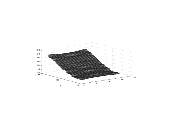
Figure 2. The chaotic dynamics in subsection 5.2 ($u$-plot).

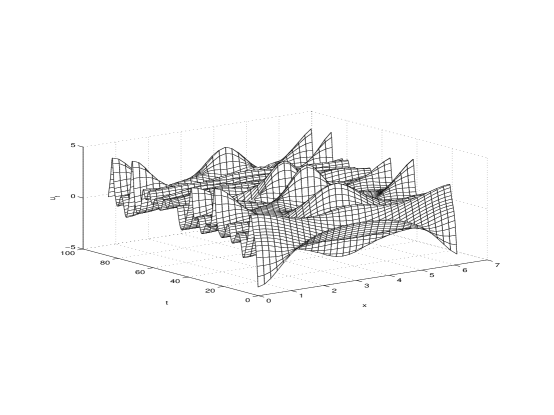
Figure 3. The chaotic dynamics in subsection 5.2 ($u_{t}$-plot).

5.3. Homoclinic Type Connection Search

To search for the homoclinic type connection near $u_{+}=0$, we need to calculate the Melnikov integral (which measures the intersection between $W^{cu}_{+}$ and $W^{cs}_{+}$):

(5.5) $$M=\int_{-\infty}^{+\infty}\int_{0}^{2\pi}\left\{\frac{\partial F_{1}}{\partial u_{t}}\left[-\alpha u_{t}+\gamma+a\sin\omega t\right]\right\}\bigg{|}_{u=u_{1}}dxdt,$$

where $u_{1}$ is given in (3.7), $\frac{\partial F_{1}}{\partial u_{t}}$ is given by (3.4) where $\Phi$ is now given by (3.8).

$$M=\alpha M^{(\alpha)}+\gamma M^{(\gamma)}+a\cos(\omega\hat{\rho}/\sigma)M^{(c)}+a\sin(\omega\hat{\rho}/\sigma)M^{(s)},$$

where

$$M^{(\alpha)} = -\frac{1}{\sigma}\int_{-\infty}^{+\infty}\int_{0}^{2\pi}\left\{\frac{\partial F_{1}}{\partial u_{t}}u_{t}\right\}\bigg{|}_{u=u_{1}}dxd\hat{\tau},$$

$$M^{(\gamma)} = \frac{1}{\sigma}\int_{-\infty}^{+\infty}\int_{0}^{2\pi}\left\{\frac{\partial F_{1}}{\partial u_{t}}\right\}\bigg{|}_{u=u_{1}}dxd\hat{\tau},$$

$$M^{(c)} = \frac{1}{\sigma}\int_{-\infty}^{+\infty}\int_{0}^{2\pi}\left\{\frac{\partial F_{1}}{\partial u_{t}}\sin(\omega\hat{\tau}/\sigma)\right\}\bigg{|}_{u=u_{1}}dxd\hat{\tau},$$

$$M^{(s)} = \frac{1}{\sigma}\int_{-\infty}^{+\infty}\int_{0}^{2\pi}\left\{\frac{\partial F_{1}}{\partial u_{t}}\cos(\omega\hat{\tau}/\sigma)\right\}\bigg{|}_{u=u_{1}}dxd\hat{\tau}.$$

As before, $M^{(\gamma)}=0$. It turns out that both $M^{(c)}$ and $M^{(s)}$ are zero (in fact $\frac{\partial F_{1}}{\partial u_{t}}_{u=u_{1}}$ has zero spatial mean). Thus there is no nontrivial solution to $M=0$. This shows a failure in searching for a persistent homoclinic orbit. Our numerical simulations indicate that there is no chaos of the type associated with homoclinic orbits.

6. The Case of $f=-\alpha u_{t}+\gamma\cos x+a\sin\omega t$

In this case, there is no guarantee that the ($\epsilon=0$) fixed point $u=u_{t}=0$ will persist into a periodic orbit. The existence of heteroclinic orbits and chaos is a far more open problem than the case in the previous section. Again consider the extended system,

$$\left\{\begin{array}[]{l}u_{tt}=c^{2}u_{xx}+\sin u+\epsilon[-\alpha u_{t}+\gamma\cos x+a\sin\theta],\cr\dot{\theta}=\omega.\cr\end{array}\right.$$

When $\epsilon=0$, the periodic orbit $u=u_{t}=0$, $\theta\in\mathbb{T}^{1}$ has two unstable eigenvalues, two stable eigenvalues, and the rest neutral eigenvalues. This leads to the following invariant manifold theorem.

Theorem 6.1.

When $c\in(1/2,1)$ and $\epsilon\geq 0$ is sufficiently small, there are a $2$ co-dimensional $C^{m}$ ($m\geq 3$) center-unstable manifold $W^{cu}_{\pm}$, a $2$ co-dimensional $C^{m}$ center-stable manifold $W^{cs}_{\pm}$, and a $4$ co-dimensional $C^{m}$ center manifold $W^{c}_{\pm}$ in the neighborhoods of $u=0,2\pi$; $u_{t}=0$, $\theta\in\mathbb{T}^{1}$ (where $u=0$ corresponds to ‘$+$’ and $u=2\pi$ corresponds to ‘$-$’) in the phase space ($u,u_{t},\theta$) $\in H^{n+1}\times H^{n}\times\mathbb{T}^{1}$ ($n\geq 1$). $W^{c}_{\pm}=W^{cu}_{\pm}\cap W^{cs}_{\pm}$. With $W^{c}_{\pm}$ as the base, $W^{cu}_{\pm}$ and $W^{cs}_{\pm}$ are fibered by $2$-dimensional Fenichel fibers.

6.1. Heteroclinic Cycle Type Connection Search

Melnikov integrals can detect orbits in $W^{cu}_{\pm}\cap W^{cs}_{\mp}$. Unfortunately both the forward and the backward destinies of such orbits are unknown. The Melnikov integrals are given by

$$M_{j\ell} = \int_{-\infty}^{+\infty}\int_{0}^{2\pi}\left\{\frac{\partial F_{\ell}}{\partial u_{t}}\left[-\alpha u_{t}+\gamma\cos x+a\sin\omega t\right]\right\}\bigg{|}_{u=u_{j}}dxdt$$

$$= \alpha M_{j\ell}^{(\alpha)}+\gamma M_{j\ell}^{(\gamma)}+a\cos(\omega\rho)M_{j\ell}^{(c)}+a\sin(\omega\rho)M_{j\ell}^{(s)},$$

where ($j=1,2;\ \ell=0,1$) and $u_{j}$’s are given in (3.1)-(3.2), $M_{j\ell}^{(\cdot)}$ are functions of $c$ and $\Delta\rho=\hat{\rho}-\sigma\rho$, $M_{j\ell}^{(c)}$ and $M_{j\ell}^{(s)}$ also depend on $\omega$, and specifically

$$M_{j\ell}^{(\alpha)} = -\int_{-\infty}^{+\infty}\int_{0}^{2\pi}\left\{\frac{\partial F_{\ell}}{\partial u_{t}}u_{t}\right\}\bigg{|}_{u=u_{j}}dxd\tau,$$

$$M_{j\ell}^{(\gamma)} = \int_{-\infty}^{+\infty}\int_{0}^{2\pi}\left\{\frac{\partial F_{\ell}}{\partial u_{t}}\cos x\right\}\bigg{|}_{u=u_{j}}dxd\tau,$$

$$M_{j\ell}^{(c)} = \int_{-\infty}^{+\infty}\int_{0}^{2\pi}\left\{\frac{\partial F_{\ell}}{\partial u_{t}}\sin(\omega\tau)\right\}\bigg{|}_{u=u_{j}}dxd\tau,$$

$$M_{j\ell}^{(s)} = \int_{-\infty}^{+\infty}\int_{0}^{2\pi}\left\{\frac{\partial F_{\ell}}{\partial u_{t}}\cos(\omega\tau)\right\}\bigg{|}_{u=u_{j}}dxd\tau.$$

It turns out from numerical calculations that all the integrals $M_{j\ell}^{(\alpha)}$, $M_{j\ell}^{(\gamma)}$, $M_{j\ell}^{(c)}$ and $M_{j\ell}^{(s)}$ are real and independent of $j$. The other integrals are the same as in previous section. Thus, the common zero of $M_{j\ell}$ satisfies the system

(6.1) $$\alpha M_{10}^{(\alpha)}+\gamma M_{10}^{(\gamma)}+a\cos(\omega\rho)M_{10}^{(c)}+a\sin(\omega\rho)M_{10}^{(s)}=0,$$

(6.2) $$\alpha M_{11}^{(\alpha)}+\gamma M_{11}^{(\gamma)}+a\cos(\omega\rho)M_{11}^{(c)}+a\sin(\omega\rho)M_{11}^{(s)}=0,$$

(6.3) $$\alpha M_{10}^{(\alpha)}+\gamma M_{10}^{(\gamma)}+a\cos(\omega\rho)M_{10}^{(c)}+a\sin(\omega\rho)M_{10}^{(s)}=0,$$

(6.4) $$\alpha M_{11}^{(\alpha)}+\gamma M_{11}^{(\gamma)}+a\cos(\omega\rho)M_{11}^{(c)}+a\sin(\omega\rho)M_{11}^{(s)}=0.$$

Notice that equations (6.3)-(6.4) are identical with equations (6.1)-(6.2). This degeneracy prohibits the application of the implicit function theorem in measuring the intersection between $W^{cu}_{\pm}$ and $W^{cs}_{\mp}$. So we have no conclusion as whether or not $W^{cu}_{\pm}$ and $W^{cs}_{\mp}$ can simultaneously intersect.

We conducted a numerical simulation of the dynamics with the following setup:

$$\epsilon=0.1,a=5.1,\omega=1.0,c=0.75,\alpha=0.257,\gamma=3.0;$$

and $64$ elements are used to divide the spatial period [$0,2\pi$], the time step is 1/40 of the forcing period $\frac{2\pi}{\omega}=2\pi$, finally the initial condition is given by (3.1) with ($t=0$, $\rho=0$, $\hat{\rho}=0$, hence $\Delta\rho=0$). The numerical result indicates chaotic dynamics as shown in Figure 4. In fact, it seems that the chaotic dynamics loops around the eye in Figure 1, i.e. around a cycle, rather than monotonely travels up to different eyes as in Figure 2. Possible explanation is that the chaotic dynamics is induced by persistent heteroclinic cycles even though our Melnikov calculation above has no conclusion.

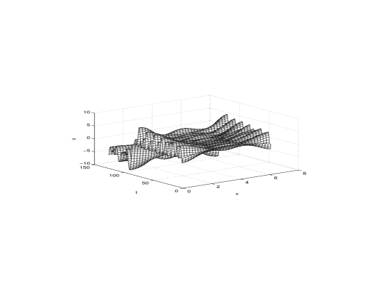
Figure 4. The chaotic dynamics in subsection 6.1.

6.2. Heteroclinic Orbit Type Connection Search

Next we shall search for an intersection between $W^{cu}_{+}$ and $W^{cs}_{-}$ (or $W^{cu}_{-}$ and $W^{cs}_{+}$) only, in which case we only need to solve equations (6.1)-(6.2). Eliminating $\alpha$, we have

$$\gamma A+a\cos(\omega\rho)B+a\sin(\omega\rho)C=0,$$

where

$$A = M_{10}^{(\gamma)}M_{11}^{(\alpha)}-M_{11}^{(\gamma)}M_{10}^{(\alpha)},$$

$$B = M_{10}^{(c)}M_{11}^{(\alpha)}-M_{11}^{(c)}M_{10}^{(\alpha)},$$

$$C = M_{10}^{(s)}M_{11}^{(\alpha)}-M_{11}^{(s)}M_{10}^{(\alpha)}.$$

Thus as long as $B$ and $C$ are not simultaneously zero, there are always non-trivial solutions:

$$\sin(\omega\rho+\theta_{1})=-\frac{\gamma A}{a\sqrt{B^{2}+C^{2}}},$$

where

$$\sin\theta_{1}=\frac{B}{\sqrt{B^{2}+C^{2}}},\quad\cos\theta_{1}=\frac{C}{\sqrt{B^{2}+C^{2}}}.$$

So we get the criterion that when

(6.5) $$|a|>\chi|\gamma|,\quad\text{where }\chi=\frac{|A|}{\sqrt{B^{2}+C^{2}}};$$

there is a heteroclinic orbit. The values of $\chi$ is shown in Table 3.

$$\begin{array}[]{|c|c|c|c|c|c|}\hline\cr\Delta\rho&-10&-5&0&5&10\\ \hline\cr\omega=0.1&36.05&1.27&2.35&1.27&36.05\\ \hline\cr\omega=0.5&47.17&1.67&1.44&1.67&47.17\\ \hline\cr\omega=1.0&89.36&3.16&1.64&3.16&89.36\\ \hline\cr\omega=2.0&413.3&14.59&25.23&14.59&413.3\\ \hline\cr\omega=3.0&1985.&69.93&105.9&69.93&1985.\\ \hline\cr\omega=4.0&9411.&327.2&387.8&327.2&9411.\\ \hline\cr\omega=5.0&45950.&1538&1214.&1538.&45950.\\ \hline\cr\end{array}$$

Table 3. The table of $\chi$ for the heteroclinic orbit case in subsection 6.2, $c=0.75$.

The chaotic dynamics in Figure 4 is in the parameter regime predicted by (6.5)

6.3. Homoclinic Type Connection Search

To search for the homoclinic type connection near $u_{+}=0$, we need to calculate the Melnikov integral (which measures the intersection between $W^{cu}_{+}$ and $W^{cs}_{+}$):

(6.6) $$M=\int_{-\infty}^{+\infty}\int_{0}^{2\pi}\left\{\frac{\partial F_{1}}{\partial u_{t}}\left[-\alpha u_{t}+\gamma\cos x+a\sin\omega t\right]\right\}\bigg{|}_{u=u_{1}}dxdt,$$

where $u_{1}$ is given in (3.7), $\frac{\partial F_{1}}{\partial u_{t}}$ is given by (3.4) where $\Phi$ is now given by (3.8).

$$M=\alpha M^{(\alpha)}+\gamma M^{(\gamma)}+a\cos(\omega\hat{\rho}/\sigma)M^{(c)}+a\sin(\omega\hat{\rho}/\sigma)M^{(s)},$$

where

$$M^{(\alpha)} = -\frac{1}{\sigma}\int_{-\infty}^{+\infty}\int_{0}^{2\pi}\left\{\frac{\partial F_{1}}{\partial u_{t}}u_{t}\right\}\bigg{|}_{u=u_{1}}dxd\hat{\tau},$$

$$M^{(\gamma)} = \frac{1}{\sigma}\int_{-\infty}^{+\infty}\int_{0}^{2\pi}\left\{\frac{\partial F_{1}}{\partial u_{t}}\cos x\right\}\bigg{|}_{u=u_{1}}dxd\hat{\tau},$$

$$M^{(c)} = \frac{1}{\sigma}\int_{-\infty}^{+\infty}\int_{0}^{2\pi}\left\{\frac{\partial F_{1}}{\partial u_{t}}\sin(\omega\hat{\tau}/\sigma)\right\}\bigg{|}_{u=u_{1}}dxd\hat{\tau},$$

$$M^{(s)} = \frac{1}{\sigma}\int_{-\infty}^{+\infty}\int_{0}^{2\pi}\left\{\frac{\partial F_{1}}{\partial u_{t}}\cos(\omega\hat{\tau}/\sigma)\right\}\bigg{|}_{u=u_{1}}dxd\hat{\tau}.$$

As before, $M^{(c)}$ and $M^{(s)}$ are zero, but now $M^{(\gamma)}$ is not zero. So $M=0$ implies that

$$\gamma=\chi\alpha,\text{ where }\chi=-M^{(\alpha)}/M^{(\gamma)}.$$

When $c=0.75$, we found that

$$\chi=-6762.7.$$

That is, comparing to the shunt loss amplitude $\alpha$, the AC current field amplitude $\gamma$ needs to be quite large to generate possible homoclinic chaotic current (CC).

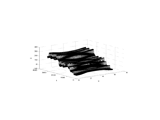
Figure 5. The chaotic dynamics in subsection 6.3.

We conducted a numerical simulation of the dynamics with the following setup:

$$\epsilon=0.01,a=0,\omega=0.55,c=0.75,\alpha=0.001,\gamma=-6.7627;$$

and $32$ elements are used to divide the spatial period [$0,2\pi$], the time step is $1/80$ of the forcing period $\frac{2\pi}{\omega}$, finally the initial condition is given by (3.1) with ($t=0$, $\rho=0$, $\hat{\rho}=0$, hence $\Delta\rho=0$). The numerical result indicates chaotic dynamics as shown in Figure 5. This chaos is still jumping around the heteroclinic loops, nevertheless most of the time it loops very close to the homoclinic orbits.

7. The Components of the Global Attractor and the Bifurcation in the Perturbation Parameter

Here we study the case of $f=-\alpha u_{t}+\gamma+a\sin\omega t$ in (1.1) which was also studied in section 5. The setup is as follows:

(7.1) $$a=1.0,\omega=0.55,c=0.75,\alpha=0.257,\gamma=0.5;$$

and $64$ elements are used to divide the spatial period [$0,2\pi$], the time step is $1/40$ of the forcing period $\frac{2\pi}{\omega}$.

The perturbed sine-Gordon system (1.1) has a global attractor up to the translation $u\rightarrow u+2\pi$ [7]. Here we are interested in the detailed structure of the global attractor. In particular, we are interested in the local attractors inside the global attractor. Components other than the local attractors, often can only attract measure zero sets of initial conditions. Figure 6 shows two local attractors inside the global attractor when $\epsilon=0.1$. For the initial condition ($u^{*},u^{*}_{t}$) given by (3.1) with $t=0$, $\rho=0$, $\hat{\rho}=0$ (hence $\Delta\rho=0$, and $u^{*}=\pi$); the solution approaches the chaotic attractor Figure 6(a). For the initial condition

$$(\hat{u},\hat{u}_{t})=(\pi,0.1+0.01r(x))$$

where $r(x)$ is a random function depending on $x$; the solution approaches the periodic attractor Figure 6(b).

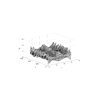
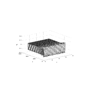
Figure 6. Two local attractors inside the global attractor. (a) is a chaotic attractor, and (b) is a periodic attractor.

To explore the initial conditions more systematically, we use the following homotopic initial conditions

$$(u,u_{t})=(1-A)(u^{*},u^{*}_{t})+A(\tilde{u},\tilde{u}_{t})$$

where $A\in[0,1]$ and $(\tilde{u},\tilde{u}_{t})=(\pi,0.1)$ i.e. we dropped the random perturbation in ($\hat{u},\hat{u}_{t}$), which does not seems to affect the final attractor. Another topic that we are interested in is the bifurcation in the perturbation parameter $\epsilon$. By combining the two parameters $\epsilon$ and $A$, we obtain the component-bifurcation diagram (Table 4), where H is the heteroclinic orbit given by (3.1), Q is the quasiperiodic solution of the integrable sine-Gordon equation ($\epsilon=0$). U is spatially uniform and temporally periodic attractor as depicted in Figure 6(b). It is originated from the integrable steady state $(u,u_{t})=(\pi,0)$ and modulated by the temporally periodic forcing $a\sin\omega t$. $B_{+}$ is a breather attractor as depicted in Figure 7. It is originated from the center of a loop of one of the small figure-eights in Figure 1 and modulated by the perturbation. $B_{-}$ is a breather attractor similar to $B_{+}$ except that the hump is located at the spatial periodic boundary. It is orginated from the center of the other loop of the small figure-eight. C is the chaotic attractor as depicted in Figure 6(a). When the value of $\epsilon$ or $A$ is larger than those in Table 4, the attractor is always U. From Table 4, one can see that there is no clear boundary between chaos attractor and regular attractor in the ($\epsilon,A$)-plane. The chaotic attractors appear and disappear in an irregular fashion when the parameters are varying. In the perturbation parameter $\epsilon$, the bifurcation does not follow any simple bifurcation paradigm in low dimensional systems.

$\epsilon$	$A=0.00$	$A=0.05$	$A=0.10$	$A=0.15$	$A=0.20$
$0$	H	Q	Q	Q	Q
$0.01$	U	$B_{-}$	U	U	U
$0.02$	U	U	U	U	U
$0.03$	$B_{+}$	U	U	U	U
$0.04$	C	C	C	U	U
$0.05$	C	C	U	U	U
$0.06$	U	C	U	U	U
$0.07$	C	C	U	U	U
$0.08$	C	U	C	U	U
$0.09$	U	C	C	U	U
$0.1$	C	U	U	U	U

Table 4. The component-bifurcation diagram in section 7. $H$: heteroclinic orbit, $Q$: quasiperiodic orbit, $U$: spatially uniform and temporally periodic attractor, $B_{+},B_{-}$: breather attractors, $C$: chaotic attractor.

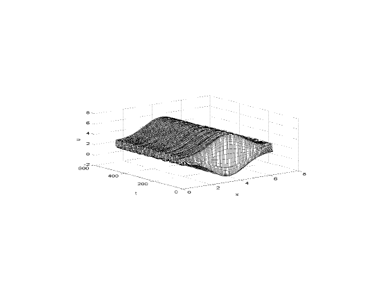
Figure 7. The breather attractor $B_{+}$ in Table 4.

8. Ratchet Effects

The long Josephson vortex ratchet effect refers to the effect of nonzero temporal average of the voltage output $u_{t}$ when the temporal part of the input forcing $f$ (1.1) has a zero temporal average. There has been a lot of recent interest on the Josephson vortex ratchet, see [4] and the references therein. Here we will study the following form of the input forcing $f$ (1.1):

(8.1) $$f=-\alpha u_{t}+g(x)+a\sin\omega t,$$

where $g(x)$ is a spatially periodic current field of zero mean. It turns out that the existence of the ratchet effect depends on whether or not the spatial potential $G$ ($G_{x}=g$) is symmetric as observed experimentally [4].

First we study the asymmetric potential case:

$$g(x)=\gamma\ \ \text{for }|x-\pi|\leq\frac{\pi}{48};\quad-\frac{\gamma}{47}\ \ \text{for other }x\in[0,2\pi].$$

Figure 8 corresponds to the following setup:

(8.2) $$\epsilon=0.1,a=2.0,\omega=0.55,c=0.75,\alpha=0.14,\gamma=100;$$

and $64$ elements are used to divide the spatial period [$0,2\pi$], the time step is $1/40$ of the forcing period $\frac{2\pi}{\omega}$, finally the initial condition is given by (3.1) with ($t=0$, $\rho=0$, $\hat{\rho}=0$, hence $\Delta\rho=0$); the temporal average of $u_{t}$ is done over 256 data points, i.e. 6.4 [256/40] times of the forcing period $\frac{2\pi}{\omega}$. One can see a clear nonzero temporal average of the voltage $u_{t}$ at $x=0$. That is, there is a clear ratchet effect. The spatio-temporal profile of $u_{t}$ is clearly chaotic in time, while the spatio-temporal profile of $u$ is also chaotic and dominated by drifting in time.

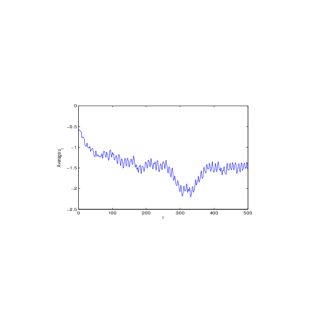
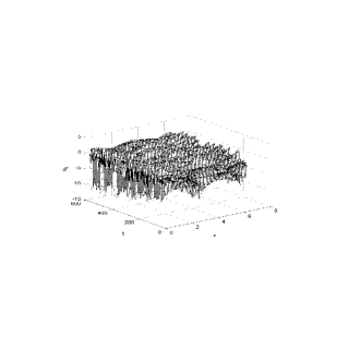
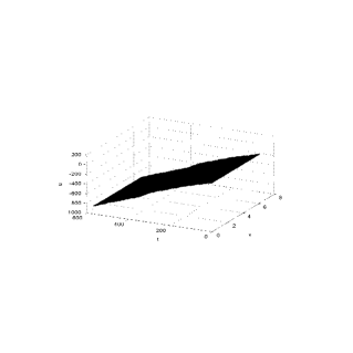
Figure 8. The temporal average of $u_{t}$ at $x=0$ is shown in (a), while (b) and (c) are spatial-temporal profiles. This is the ratchet effect in the asymmetric potential case.

Next we study the symmetric potential case: $g(x)=\gamma\cos x$ which is the case studied in Section 6. Figure 9 corresponds to the same setup as (8.2) and the rest. One can see that the temporal average of the voltage $u_{t}$ at $x=0$ is approaching zero in time.That is, there is no ratchet effect in long term. The spatio-temporal profile of $u_{t}$ is transiently chaotic in time, while the spatio-temporal profile of $u$ is also transiently chaotic in time and its drifting in time is mild.

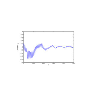
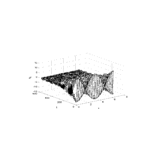
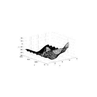
Figure 9. The temporal average of $u_{t}$ at $x=0$ is shown in (a), while (b) and (c) are spatial-temporal profiles. This corresponds to no ratchet effect in the symmetric potential case.

Figure 10 corresponds to the same setup as (8.2) and the rest except $a=5.0$. One can see that the temporal average of the voltage $u_{t}$ at $x=0$ is also slowly approaching zero in time. That is, there is no ratchet effect in long term. The spatio-temporal profile of $u_{t}$ is transiently chaotic in time with a longer term, while the spatio-temporal profile of $u$ is also transiently chaotic in time and it almost has no drifting in time.

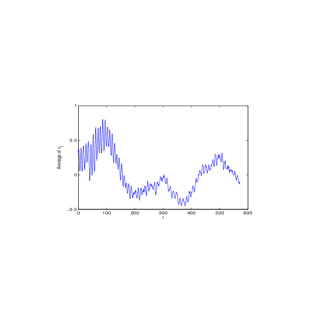
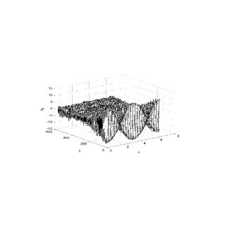
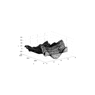
Figure 10. The temporal average of $u_{t}$ at $x=0$ is shown in (a), while (b) and (c) are spatial-temporal profiles. This also corresponds to no ratchet effect in the symmetric potential case. The difference from Figure 9 is that the value of the parameter $a$ is different.

9. Conclusion and Discussion

Via a combination of numerical and Melnikov integral studies, we find that DC current bias cannot induce chaotic flux dynamics, while AC current bias can. The existence of a common root to the Melnikov integrals is a necessary condition for the existence of chaotic flux dynamics. The global attractor can contain co-existing local attractors e.g. a local chaotic attractor and a local regular attractor. In the infinite dimensional phase space setting, the bifurcation is very complicated. Chaotic attractors can appear and disappear in a random fashion. In the parameter space, there is no clear regular boundary between local chaotic attractors and local regular attractors. Three types of attractors (chaos, breather, spatially uniform and temporally periodic attractor) are identified. Ratchet effect can be achieved by a current bias field which corresponds to an asymmetric potential as observed in experiments [4], in which case the flux dynamics is ever lasting chaotic. When the current bias field corresponds to a symmetric potential, the flux dynamics is often transiently chaotic, in which case the ratchet effect disappears after sufficiently long time.

Due to its infinite dimensionality, numerically exploring the entire phase space is impossible. Here we focus upon an interesting neighborhood. It is entirely possible that other novel structures are hidden somewhere else in the phase space. Also due to the infinite dimensionality, the link between existence of chaos (and homoclinic orbit) and existence of a common root to the Melnikov integrals becomes weaker. Finally, chaos in the infinite diemsional phase space is often transient. After sufficiently long time, the seemingly chaotic dynamics may converge to a regular attractor.

Inside the global attractor, there may be many invariant components. An interesting topic is to classify these components. Of particular interest are those components which are local attractors. Some local attractors may be chaotic, while others may be regular. Different initial conditions may lead to different local attractors. A complete classification of all these local attractors is very challenging, especially in the infinite dimensional setting. This article only explores a selected set of initial conditions. When the value of the perturbation parameter changes, the dynamics undergoes bifurcations. Unlike in low dimensional systems, bifurcations in the infinite dimensional system are much more complicated.

References

- [1] G. Augello, et al., Lifetime of the superconductive state in short and long Josephson junctions, Eur. Phys. J. B (2009), e-00155.
- [2] F. Barkov, M. Fistul, A. Ustinov, Microwave-induced flow of vortices in long Josephson junctions, Phys. Rev. B 70 (2004), 134515.
- [3] A. Barone, G. Paterno, Physics and Applications of the Josephson Effect, Wiley & Sons, 1982.
- [4] M. Beck, et al., High efficiency deterministic Josephson vortex ratchet, Phys. Rev. Lett. 95 (2005), 090603.
- [5] J. van den Berg, S. van Gils, T. Visser, Parameter dependence of homoclinic solutions in a single long Josephson junction, Nonlinearity 16 (2003), 707.
- [6] T. Boyadjiev, et al., Created-by-current states in long Josephson junctions, EPL 83 (2008), 47008.
- [7] V. Chepyzhov, M. Vishik, Attractors for Equations of Mathematical Physics, AMS Colloquium Publications, vol.49, 2002.
- [8] W. Johnson, Nonlinear wave propagation on superconducting tunneling junctions, Ph.D. Thesis, University of Wisconsin, Madison (1968).
- [9] B. Josephson, The discovery of tunnelling supercurrents, Rev. Mod. Phys. 46(2) (1974), 251-254.
- [10] Y. Kasai, et al., Fluxon dynamics in isolated long Josephson junctions, Physica C: Superconductivity 352 (2001), 211-214.
- [11] U. Kienzle, et al., Thermal escape of fractional vortices in long Josephson junctions, arXiv:0903.3382 (2009).
- [12] Y. Li, Chaos in Partial Differential Equations, International Press, 2004.
- [13] Y. Li, Chaos and shadowing lemma for autonomous systems of infinite dimensions, J. Dyn. Diff. Eq. 15, no.4 (2003), 699-730.
- [14] Y. Li, Chaos and shadowing around a homoclinic tube, Abstract and Applied Analysis 2003, no.16 (2003), 923-931.
- [15] Y. Li, Homoclinic tubes and chaos in perturbed sine-Gordon equation, Chaos, Solitons and Fractals 20, no.4 (2004), 791-798.
- [16] Y. Li, Chaos and shadowing around a heteroclinically tubular cycle with an application to sine-Gordon equation, Studies in Applied Mathematics 116 (2006), 145-171.
- [17] Y. Li, D. McLaughlin, Morse and Melnikov functions for NLS pde’s, Comm. Math. Phys. 162 (1994), 175-214.
- [18] Y. Li, et al., Persistent homoclinic orbits for perturbed nonlinear Schrödinger equation, Comm. Pure and Appl. Math. XLIX (1996), 1175-1255.
- [19] Y. Li, Smale horseshoes and symbolic dynamics in perturbed nonlinear Schrödinger equations, J. of Nonlinear Sci. 9 (1999), 363-415.
- [20] Y. Li, Persistent homoclinic orbits for nonlinear Schrödinger equation under singular perturbation, Dynamics of PDE 1, no.1 (2004), 87-123.
- [21] Y. Li, Existence of chaos for nonlinear Schrödinger equation under singular perturbation, Dynamics of PDE 1, no.2 (2004), 225-237.
- [22] A. Pankratov, Long Josephson junctions with spatially inhomogeneous driving, Phys. Rev. B 66 (2002), 134526.
- [23] H. Rauh, et al., Nonlocal fluxon dynamics in long Josephson junctions with Newtonian dissipative loss, J. Phys.: Condens. Matter 16 (2004), S2715-2733.
- [24] P. Shaju, V. Kuriakose, Double-well potential in annular Josephson junction, Phys. Lett. A 332 (2004), 326-332.
- [25] A. Soblev, et al., Numerical simulation of the self-pumped long Josephson junction using a modified sine-Gordon model, Physica C: Superconductivity 435 (2006), 112-113.
- [26] I. Tornes, Critical current calculations for long Josephson junction, Eur. Phys. J. B 59 (2007), 485-493.