On Almost-Fuchsian Manifolds

Abstract.

Almost-Fuchsian manifold is a class of complete hyperbolic three-manifolds. Such a three-manifold is a quasi-Fuchsian manifold which contains a closed incompressible minimal surface with principal curvatures everywhere in the range of $(-1,1)$. In such a manifold, the minimal surface is unique and embedded, hence one can parametrize these hyperbolic three-manifolds by their minimal surfaces. In this paper we obtain estimates on several geometric and analytical quantities of an almost-Fuchsian manifold $M$ in terms of the data on the minimal surface. In particular, we obtain an upper bound for the hyperbolic volume of the convex core of $M$, and an upper bound on the Hausdorff dimension of the limit set associated to $M$. We also constructed a quasi-Fuchsian manifold which admits more than one minimal surface, and it does not admit a foliation of closed surfaces of constant mean curvature.

1. Introduction

Quasi-Fuchsian manifold is an important class of complete hyperbolic three-manifolds. In hyperbolic geometry, quasi-Fuchsian manifolds and their moduli space, the quasi-Fuchsian space $\mathcal{Q\!F}(S)$, have been objects of extensive study in recent decades. In particular, incompressible surfaces of small principal curvatures play an important role in hyperbolic geometry and low dimensional topology ([Rub05]). Analogs of these surfaces and three-manifolds are also a center of study in anti-de-Sitter geometry ([KS07, Mes07]). In this paper, we mostly consider a subspace of the quasi-Fuchsian space: almost-Fuchsian manifolds. They form a subspace of the same complex dimension $6g-6$ in $\mathcal{Q\!F}(S)$, where $g\geq 2$ is the genus of any closed incompressible surface in the manifold ([Uhl83]). Understanding the structures of the quasi-Fuchsian space is a mixture of understanding the geometry of quasi-Fuchsian $3$-manifolds, the deformation of incompressible surfaces, as well as the representation theory of Kleinian groups. It is highly desirable to use information on special surfaces (minimal or constant mean curvature) to obtain global information on the three-manifold.

Let us make a definition: Definition: We call $M$ an almost-Fuchsian manifold if it is a quasi-Fuchsian manifold which contains a closed incompressible minimal surface $\Sigma$ such that the principal curvatures of $\Sigma$ are in the range of $(-1,1)$. Recall that we call a closed surface incompressible in $M$ if the inclusion induces an injection between fundamental groups of the surface and the three-manifold $M$. Naturally, $M$ is Fuchsian when $\Sigma$ is actually totally geodesic. The notion of almost-Fuchsian (term coined in [KS07]) was first studied by Uhlenbeck ([Uhl83]), where she proved several key properties of almost-Fuchsian manifolds that will be vital in this work: $\Sigma$ is the only closed incompressible minimal surface in $M$, and $M$ admits a foliation of parallel surfaces from $\Sigma$ to both ends. Around the same time, Epstein ([Eps86]) used the parallel flow in $\mathbb{H}^{3}$ to study the quasiconformal reflection problem.

Throughout the paper, all surfaces in $M$ involved are assumed to be closed, oriented, incompressible, of genus at least two. We also assume $M$ is not Fuchsian, or most theorems are trivial. One of our motivations is to use various techniques in analysis to investigate geometric problems in hyperbolic three-manifolds.

Since the minimal surface is unique in an almost-Fuchsian manifold, we can use minimal surfaces to parametrize the space of almost-Fuchsian manifolds. This parametrization is in terms of the conformal structure of the minimal surface and the holomorphic quadratic differential on the conformal structure which determines the second fundamental form of the minimal surface in the three-manifold (see [Uhl83, Tau04, HL12]). We will focus on instead obtaining topological and geometric information about $M$ from data of $\Sigma$ in this paper. Among the quantities associated to a quasi-Fuchsian manifold, the hyperbolic volume of the convex core and the Hausdorff dimension of the limit set are perhaps the most significant. Estimates on them in term of the geometry of the minimal surface in $M$ are obtained in this paper. Moreover, the foliation structure possessed by $M$ allows us to investigate a notion of renormalized volume for the almost-Fuchsian manifold.

The convex core of a quasi-Fuchsian manifold is the smallest convex subset of a quasi-Fuchsian manifold that carries its fundamental group. From the point of view of hyperbolic geometry, the convex core contains all the geometrical information about the quasi-Fuchsian three-manifold itself (see for instance, [AC96, Bro03]). As a direct application, when $M$ is almost-Fuchsian, we obtain an explicit upper bound for the hyperbolic volume of the convex core $C(M)$, in terms of the maximum principal curvature on the minimal surface $\Sigma$:

Theorem 1.1.

If $M$ is almost-Fuchsian, and let $\lambda_{0}=\max\limits_{x\in\Sigma}\{|\lambda(x)|\}$ be the maximum of the principal curvature of the minimal surface $\Sigma$ of $M$, then

$$\operatorname{Vol}(C(M)) \leq\mathcal{A}_{\operatorname{hyp}}\left({\frac{\lambda_{0}}{1-\lambda_{0}^{2}}}+{\frac{1}{2}}\log{\frac{1+\lambda_{0}}{1-\lambda_{0}}}\right)$$

(1.1) $$=\mathcal{A}_{\operatorname{hyp}}\left(2\lambda_{0}+{\frac{4}{3}}\lambda_{0}^{3}+O(\lambda_{0}^{5})\right),$$

where $\mathcal{A}_{\operatorname{hyp}}=2\pi(2g-2)$ is the hyperbolic area of $\Sigma$.

We immediately see quantitatively how the volume of $C(M)$ goes to zero when $\lambda_{0}$ is close to zero. In [Bro03], Brock showed the hyperbolic volume of the convex core is quasi-isometric to the Weil-Petersson distance between conformal infinities of $M$ in Teichmüller space.

It is well-known that the Hausdorff dimension of the limit set for any quasi-Fuchsian group is in the range of $[1,2)$, and identically $1$ if and only if it is Fuchsian. We also obtain an upper bound for the Hausdorff dimension of the limit set $\Lambda_{\Gamma}$ of $M$, in terms of $\lambda_{0}$ as well:

Theorem 1.2.

If $M=\mathbb{H}^{3}/\Gamma$ is almost-Fuchsian, and let $\lambda_{0}=\max\limits_{x\in\Sigma}\{|\lambda(x)|\}$, then the Hausdorff dimension $D(\Lambda_{\Gamma})$ of the limit set $\Lambda_{\Gamma}$ for $M$ satisfies

(1.2) $$D(\Lambda_{\Gamma})<1+\lambda_{0}^{2}.$$

For $\lambda_{0}$ close to zero, Theorems 1.1 and 1.2 measure how close $M$ is to being Fuchsian. In ([GHW10]), we related the foliation structure of an almost-Fuchsian manifold to both Teichmüller metric and the Weil-Petersson metric on Teichmüller space.

Given a quasi-Fuchsian manifold, it admits finitely number of minimal surfaces ([And83]). One expects the space of almost-Fuchsian manifolds is not the full quasi-Fuchsian space, and indeed, the second named author ([Wan12]) showed some quasi-Fuchsian manifolds that admit more than one minimal surface. A further generalization is to consider closed surfaces of constant mean curvature in a quasi-Fuchsian manifold. This is a vastly rich area where many analytical techniques can be applied. A natural question (Thurston) is to ask, to what extent that a quasi-Fuchsian manifold admits a foliation of closed (incompressible) surfaces of constant mean curvature. In the second part of this paper, we construct a quasi-Fuchsian manifold which admits more than one minimal surface (hence not almost-Fuchsian), such that it does not admit such a foliation, namely,

Theorem 1.3.

There exists a quasi-Fuchsian manifold $N$ which does not admit a foliation of constant mean curvature surfaces.

One of our original motivations is to investigate whether almost-Fuchsian manifolds are the appropriate subclass of quasi-Fuchsian manifolds that admit such a foliation.

We conclude this introduction by the following note: our volume estimate can be generalized to a possibly slightly larger class of quasi-Fuchsian manifolds than almost-Fuchsian manifolds. In other words, one can define a notion of nearly Fuchsian manifolds: a class of quasi-Fuchsian manifolds that each admits a closed incompressible surface (not necessarily minimal) of principal curvatures in the range of $(-1,1)$. One can similarly verify that a nearly Fuchsian manifold admits a foliation by parallel surfaces of this fixed surface of small principal curvatures. It is not known if these two classes of quasi-Fuchsian manifolds actually coincide, or if any nearly Fuchsian manifold admit only one minimal surface.

Plan of the paper

After a brief section on the preliminaries, the rest of the paper contains two parts: In §3, we prove several results on the geometry of almost-Fuchsian manifolds, including the renormalized volume of $M$, Theorem 1.1 (volume estimate) and Theorem 1.2 (Hausdorff dimension estimate). In §4, we prove Theorem 1.3 by constructing an explicit quasi-Fuchsian manifold.

Acknowledgements

The authors are grateful to Ren Guo for many helpful discussions, Dick Canary and Jun Hu for their suggestions regarding the Hausdorff dimension of the limit set. The last section is based on part of the thesis of the second named author, and he wishes to thank his advisor Bill Thurston for advices, inspiration and encouragement. We also want to express our gratitude to anonymous referee(s), for their willingness to read the paper carefully and for many suggestions to improve this paper. The research of Zheng Huang is partially supported by a PSC-CUNY research award and an award from the CUNY-CIRG program and CUNY-CSI Provost’s Scholarship.

2. Preliminaries

In this section, we fix our notations, and introduce some preliminary facts that will be used later in this paper.

2.1. Quasi-Fuchsian manifolds

For detailed reference on Kleinian groups and low dimensional topology, one can go to [Mar74] and [Thu82].

The universal cover of a complete orientable hyperbolic three-manifold is $\mathbb{H}^{3}$, and the deck transformations induce a representation of the fundamental group of the manifold in $\operatorname{Isom}(\mathbb{H}^{3})=\operatorname{PSL}(2,\mathbb{C})$, the (orientation preserving) isometry group of $\mathbb{H}^{3}$. A subgroup $\Gamma\subset\operatorname{PSL}(2,\mathbb{C})$ is called a Kleinian group if $\Gamma$ acts on $\mathbb{H}^{3}$ properly discontinuously. For any Kleinian group $\Gamma$, $\forall\,p\in\mathbb{H}^{3}$, the orbit set

$$\Gamma(p)=\{\gamma(p)\ |\ \gamma\in\Gamma\}$$

has accumulation points on the boundary $\partial\mathbb{H}^{3}=S^{2}_{\infty}=\widehat{\mathbb{C}}$, and these points are the limit points of $\Gamma$, and the closed set of all these points is called the limit set of $\Gamma$, denoted by $\Lambda_{\Gamma}$.

In the case when $\Lambda_{\Gamma}$ is contained in a circle $S^{1}\subset S^{2}$, the quotient manifold $M=\mathbb{H}^{3}/\Gamma$ is called Fuchsian, and $M$ is isometric to a (warped) product space $S\times\mathbb{R}$. If the limit set $\Lambda_{\Gamma}$ lies in a Jordan curve, the quotient three-manifold $M=\mathbb{H}^{3}/\Gamma$ is called quasi-Fuchsian, and it is topologically $S\times\mathbb{R}$, where $S$ is a closed surface of genus $g$ at least two. It is clear that a quasi-Fuchsian manifold is quasi-isometric to a Fuchsian manifold. The space of such three-manifolds $\mathcal{Q\!F}(S)$, the quasi-Fuchsian space of genus $g$ surfaces, is a complex manifold of dimension of $6g-6$, which has very complicated structures.

Finding minimal surfaces in negatively curved manifolds is a problem of fundamental importance. The basic results are due to Schoen-Yau ([SY79]) and Sacks-Uhlenbeck ([SU82]), and their results can be applied to the case of quasi-Fuchsian manifolds: any quasi-Fuchsian manifold contains at least one incompressible minimal surface. In the case of almost-Fuchsian, the minimal surface is unique ([Uhl83]). On the other hand, there are quasi-Fuchsian manifolds that admit many minimal surfaces ([Wan12]).

An essential problem in hyperbolic geometry and complex dynamics is to study the Hausdorff dimension $D(\Lambda_{\Gamma})$ of the limit set $\Lambda_{\Gamma}$ associated to $M$. This problem is also intimately related to understanding the lower spectrum theory of hyperbolic three-manifold ([Sul87, BC94]). In the case of Fuchsian manifolds, $\Lambda_{\Gamma}$ is a round circle and $D(\Lambda_{\Gamma})=1$. When $M$ is quasi-Fuchsian but not Fuchsian, as is throughout this paper, it is known that $1<D(\Lambda_{\Gamma})<2$ ([Bow79, Sul87]). There is a rich theory of quasiconformal mapping and its distortion on Hausdorff dimension, area and other quantities (see for instance [GV73, LV73]).

2.2. Almost-Fuchsian manifolds

We now assume that $M$ is an almost-Fuchsian manifold: the principal curvatures of the minimal surface $\Sigma$ are in the range of $(-1,1)$. It is clear that for any closed embedded surface $S$ in $M$, one can define a regular parallel surface $S(r)$ which is fixed (hyperbolic) distant $r$ from $S$, for sufficiently small $r$. A remarkable property for $M$ is that when taking $S$ to be the minimal surface, the parallel surface $S(r)$ is nonsingular for all $r\in\mathbb{R}$.

To be more precise, using isothermal coordinates, the induced metric on a closed incompressible surface $S$ is given by $g_{ij}(x)=e^{2v(x)}\delta_{ij}$, where $v(x)$ is a smooth function on $S$, and while the second fundamental form is denoted by $A(x)=[h_{ij}]_{2\times{}2}$, where $h_{ij}$ is given by, for $1\leq{}i,j\leq{}2$,

$$h_{ij}=\langle{{\overline{\nabla}}_{e_{i}}\nu},{e_{j}}\rangle,$$

where we choose $\{e_{1},e_{2}\}$ as an orthonormal basis on $S$, and $\nu$ is the unit normal field on $S$, and ${\overline{\nabla}}$ is the Levi-Civita connection of $(M,\bar{g}_{\alpha\beta})$. Here, we add a bar on top for each quantity or operator with respect to $(M,\bar{g}_{\alpha\beta})$.

Let $\lambda_{1}(x)$ and $\lambda_{2}(x)$ be the eigenvalues of $A(x)$. They are the principal curvatures of $S$, and we denote $H(x)=\lambda_{1}(x)+\lambda_{2}(x)$ as the mean curvature function of $S$. In classical differential geometry, the second fundamental form indicates how a hypersurface immerses into the ambient manifold. Zero second fundamental form is equivalent to say that the hypersuface is totally geodesic. Therefore, principal curvatures are natural quantities to investigate in this type of problems.

Let $S(r)$ be the family of equidistant surfaces with respect to $S$, i.e.

$$S(r)=\{\exp_{x}(r\nu)\ |\ x\in{}S\}\ ,\quad{}r\in(-\varepsilon,\varepsilon)\ .$$

The induced metric on $S(r)$ is denoted by $g(x,r)=[g_{ij}(x,r)]_{1\leq{}i,j\leq{}2}$, and the second fundamental form is denoted by $A(x,r)=[h_{ij}(x,r)]_{1\leq{}i,j\leq{}2}$. The mean curvature on $S(r)$ is thus given by $H(x,r)=g^{ij}(x,r)h_{ij}(x,r)$. Uhlenbeck calculated the induced metric on $S(r)$ in terms of the induced metric on $S$ and the second fundamental form of $S$, and found

Lemma 2.1 ([Uhl83]).

The induced metric $g(x,r)$ on $S(r)$ has the form

(2.1) $$g(x,r)=e^{2v(x)}[\cosh(r)\mathbb{I}+\sinh(r)e^{-2v(x)}A(x)]^{2}\ ,$$

where $r\in(-\varepsilon,\varepsilon)$.

Any point on the parallel surface $S(r)$ in $M$ can now be represented by a pair $(x,r)$, where $x\in S$ and $r\in(-\varepsilon,\varepsilon)$. Direct computation shows that the principal curvatures of $S(r)$ are given by

(2.2) $$\mu_{j}(x,r)=\frac{\tanh{}r+\lambda_{j}(x)}{1+\lambda_{j}(x)\tanh{}r}\ ,\qquad j=1,2\ .$$

Hence the mean curvature (the sum of principal curvatures) is given by

(2.3) $$H(x,r)=\frac{2(1+\lambda_{1}\lambda_{2})\tanh{}r+(\lambda_{1}+\lambda_{2})(1+\tanh^{2}r)}{1+(\lambda_{1}+\lambda_{2})\tanh{}r+\lambda_{1}\lambda_{2}\tanh^{2}r}\ .$$

Since $M$ is almost-Fuchsian, we now choose $S=\Sigma$ to be the unique minimal surface in $M$. From the explicit nature of the Lemma 2.1, one concludes that, when $|\lambda_{j}(x)|<1$ for $j=1,2$ and $x\in\Sigma$, the induced metrics $g(x,r)$ are of no singularity for all $r\in\mathbb{R}$ and therefore parallel surfaces of $\Sigma$ form a foliation on $M$, called the equidistant foliation or the normal flow. We also observe all principal curvatures $\{\mu_{j}(x,r)\}$ on the parallel surfaces are in the range of $(-1,1)$. We denote the equidistant foliation from the minimal surface $\Sigma$ by $\{\Sigma(r)\}_{r\in\mathbb{R}}$.

3. Geometry of Almost-Fuchsian Manifolds

In this section, we wish to obtain information about the almost-Fuchsian manifold $M$ via its unique minimal surface $\Sigma$. We derive several geometrical properties on the equidistant foliation $\{\Sigma(r)\}_{r\in\mathbb{R}}$ in §3.1. The calculations in this subsection will set up the stage for later applications. In §3.2, we obtain explicit upper bounds for the hyperbolic volume of the convex core of $M$, and compute explicitly the renormalized volume of $M$. In §3.3, we establish the estimate for the Hausdorff dimension of the limit set associated to the almost-Fuchsian manifold $M$.

3.1. Some estimates on the parallel surfaces

In this subsection, we provide several estimates that will be used later. First, let us record a few quantities that will be involved:

1. The principal curvatures of the minimal surface $\Sigma$ are $\pm\lambda(x)$, where $x\in\Sigma$ and we have $0\leq\lambda(x)<1$;

2. $\lambda_{0}$ is the maximum of $\lambda$, hence the maximal principal curvature on $\Sigma$;

3. $|S|$ is the area for any closed incompressible surface $S$ (with respect to the induced metric);

4. $\mathcal{A}_{\operatorname{hyp}}=2\pi(2g-2)$ is the hyperbolic area of any closed Riemann surface $S$;

5. $J(r)$ is the determinant of the Jacobian between $\Sigma$ and the parallel surface $\Sigma(r)$ via the pullback. Note that $\Sigma(r)$ is regular if and only if $J(r)>0$;

6. $K(r)$ is the Gaussian curvature on $\Sigma(r)$. In particular, $K(0)=K(\Sigma)$ is the Gaussian curvature on the minimal surface $\Sigma$;

7. $M(\pm r)$, $r>0$, is the region in $M$ bounded by surfaces $\Sigma(-r)$ and $\Sigma(r)$;

8. Lastly, $M(r)$, $r>0$, is the region in $M$ bounded between the minimal surface $\Sigma$ and the parallel surface $\Sigma(r)$.

We start with a well-known estimate which implies the area of the minimal surface under the induced metric from the ambient space is comparable to that of the hyperbolic area, with universal constants. We only include a proof for the sake of completeness, and it is very short.

Proposition 3.1.

$\frac{\mathcal{A}_{\operatorname{hyp}}}{2}<|\Sigma|<\mathcal{A}_{\operatorname{hyp}}$.

Proof.

We apply the Gauss equation:

$$K(\Sigma)=-1+\det(A)=-1-\lambda^{2}$$

Thus we have

$$-K(\Sigma)=1-\det(A)=1+\lambda^{2}.$$

We integrate this on the surface $\Sigma$, and apply the Gauss-Bonnet theorem, since $\Sigma$ is closed, to find

$$|\Sigma|<|\Sigma|+\int_{\Sigma}\lambda^{2}=\mathcal{A}_{\operatorname{hyp}}<2|\Sigma|.$$

∎

We next want to estimate the area of each parallel surface in the equidistant foliation $\{\Sigma(r)\}_{r\in\mathbb{R}}$. We can see that they grow at a rate of $\sinh^{2}(r)$, which is as expected. The explicit formula in Lemma 2.1 indicates, for large $|r|$, the metric for $M$ behaves like the warped product metric.

Proposition 3.2.

For all $-\infty<r<+\infty$, we have

$$(2|\Sigma|-\mathcal{A}_{\operatorname{hyp}})\sinh^{2}(r)<|\Sigma(r)|<|\Sigma|\cosh^{2}{}r<\mathcal{A}_{\operatorname{hyp}}\cosh^{2}{}r$$

Proof.

The area element of $\Sigma(r)$ is given by

(3.1) $$d\mu(r)=(\cosh^{2}{}r-\lambda^{2}(x)\sinh^{2}{}r)d\mu,$$

where $d\mu$ is the area element for the minimal surface $\Sigma$.

We can now compute the surface area:

$$|\Sigma(r)| =\int_{\Sigma}(\cosh^{2}{}r-\lambda^{2}(x)\sinh^{2}{}r)d\mu$$

$$=|\Sigma|\cosh^{2}{}r-\sinh^{2}{}r\int_{\Sigma}\lambda^{2}(x)d\mu$$

(3.2) $$=|\Sigma|\cosh^{2}{}r-(\mathcal{A}_{\operatorname{hyp}}-|\Sigma|)\sinh^{2}{}r$$

$$=|\Sigma|(\cosh^{2}{}r+\sinh^{2}{}r)-\mathcal{A}_{\operatorname{hyp}}\sinh^{2}{}r$$

(3.3) $$=|\Sigma|+(2|\Sigma|-\mathcal{A}_{\operatorname{hyp}})\sinh^{2}{}r\,$$

Here we used the identity

(3.4) $$\int_{\Sigma}\lambda^{2}=\mathcal{A}_{\operatorname{hyp}}-|\Sigma|.$$

The estimates then follows from the Proposition 3.1, formulas (3.2) and (3.3). ∎

As a consequence of the formula (3.1), we find that the determinant of the Jacobian between $\Sigma$ and $\Sigma(r)$ is

(3.5) $$J(r)=\cosh^{2}(r)-\lambda^{2}(x)\sinh^{2}(r).$$

From this, clearly, $|\lambda|<1$ implies that $J(r)>0$ for all $r\in\mathbb{R}$. We also have the following version of the Gauss-Bonnet formula:

Proposition 3.3.

The product of $J(r)$ and $K(r)$ is a function of $x\in\Sigma$, independent of $r$. In other words,

(3.6) $$J(r)K(r)=K(0)=-1-\lambda^{2}.$$

Proof.

Let us conduct this computation. The formulas for the principal curvatures of $\Sigma(r)$ are given by (2.2). Therefore we have

$$K(r) = -1+\mu_{1}(r)\mu_{2}(r)$$

$$= -1+\frac{\tanh^{2}(r)-\lambda^{2}}{1-\lambda^{2}\tanh^{2}(r)}$$

$$= \frac{(\lambda^{2}+1)(\sinh^{2}(r)-\cosh^{2}(r))}{J(r)}$$

$$= -\frac{(\lambda^{2}+1)}{J(r)}.$$

∎

We conclude this subsection with the following remark that the identity (3.6) holds more generally. If $S$ is a closed surface with principal curvatures $\{\lambda_{1}(x),\lambda_{2}(x)\}$, and $r\in\mathbb{R}$ is a real number such that $S(r)$ is a nonsingular parallel surface of $S$. Then the identity (3.6) shows that what must happen geometrically when $S(r)$ is developing a singularity: the Gaussian curvature of $S(r)$ must blow up. This was also observed in [Eps84].

3.2. The convex core volume and the renormalized volume

We obtain an upper bound for the hyperbolic volume of the convex core $C(M)$ in this subsection, in terms of the maximum, $\lambda_{0}$, of the principal curvature on the minimal surface $\Sigma$. The idea and actual computation are somewhat simple: we take advantage of the foliation structure of the almost-Fuchsian manifold $M$, and note that, from the formula (2.2), the principal curvatures of the surface $\Sigma(r)$, $\mu_{1}(x,r)$ and $\mu_{2}(x,r)$ are increasing functions of $r$ for any fixed $x\in\Sigma$, and they approach $\pm 2$ as $r\rightarrow\pm\infty$. When any of the parallel surfaces becomes convex (all positive principal curvatures or all negative principal curvatures), they lie outside of the convex core.

Naturally, we are particularly interested in two critical cases: the values of $r$ when $\mu_{1}(x,r)=0$ or $\mu_{2}(x,r)=0$. Elementary algebra shows:

Proposition 3.4.

If we denote

$$r_{0}={\frac{1}{2}}\log{\frac{1+\lambda_{0}}{1-\lambda_{0}}}\ ,$$

where $\lambda_{0}=\max\limits_{x\in S}\{\lambda(x)\}$, then $r_{0}$ is the least value of $r$ such that $\mu_{1}(r,x)>0$ for all $r>r_{0}$ and $x\in\Sigma$, while $-r_{0}$ is the largest value for $\mu_{2}(r,x)<0$ such that $\mu_{2}(r,x)<0$ for all $r<-r_{0}$ and $x\in\Sigma$.

This Proposition tells us when the parallel surfaces in the equidistant foliation $\{\Sigma(r)\}_{r\in\mathbb{R}}$ become convex, hence by the definition of the convex core, provides an upper bound for the size of the convex core.

Recalling that we denote the region of $M$ bounded between surfaces $\Sigma(-r_{0})$ and $\Sigma(r_{0})$ by $M(\pm r_{0})$, and then the convex core $C(M)$, is contained in $M(\pm r_{0})$. Since $\{\Sigma(r)\}_{r\in\mathbb{R}}$ foliates $M$, we can compute the hyperbolic volume of the region $M(\pm r_{0})$ by the following:

$$\operatorname{Vol}(M(\pm r_{0})) =\int_{-r_{0}}^{r_{0}}|\Sigma(r)|dr$$

$$=2r_{0}|\Sigma|+(2|\Sigma|-\mathcal{A}_{\operatorname{hyp}})\int_{-r_{0}}^{r_{0}}\sinh^{2}r{}dr$$

$$=2r_{0}|\Sigma|+(2|\Sigma|-\mathcal{A}_{\operatorname{hyp}})\left({\frac{1}{2}}\sinh(2r_{0})-r_{0}\right)$$

(3.7) $$=|\Sigma|\sinh(2r_{0})-\mathcal{A}_{\operatorname{hyp}}\left({\frac{1}{2}}\sinh(2r_{0})-r_{0}\right)$$

Applying the Proposition 3.2, we obtain the following:

Theorem 3.5.

The hyperbolic volume of $C(M)$ is bounded by:

(3.8) $$\operatorname{Vol}(C(M)) \leq \mathcal{A}_{\operatorname{hyp}}(\cosh{}r_{0}\sinh{}r_{0}+r_{0})$$

$$= \mathcal{A}_{\operatorname{hyp}}\left({\frac{\lambda_{0}}{1-\lambda_{0}^{2}}}+{\frac{1}{2}}\log{\frac{1+\lambda_{0}}{1-\lambda_{0}}}\right).$$

When $r_{0}=0$, or equivalently, $\lambda(x)=0$ for all $x\in\Sigma$, this is the case of $M$ being Fuchsian, and the hyperbolic volume of the convex core $C(M)$ is zero. We want to measure how the hyperbolic volumes vary for small $\lambda_{0}$ via the following Taylor series expansion:

Corollary 3.6.

For small $\lambda_{0}$, we have the following expansion:

$$\operatorname{Vol}(C(M))\leq\mathcal{A}_{\operatorname{hyp}}\left(2\lambda_{0}+{\frac{4}{3}}\lambda_{0}^{3}+O(\lambda_{0}^{5})\right).$$

Any quasi-Fuchsian manifold is complete, hence has infinite volume. It is classical in conformal geometry to define a notion of renormalized volume ([FG85, PP01]) to obtain some conformal invariant. The foliation structure of an almost-Fuchsian manifold allows one to derive a simple quantity as the renormalized volume. We adapt the following notion: the renormalized volume of $M$ with respect to the foliation $\{\Sigma(r)\}_{r\in\mathbb{R}}$ is given by

(3.9) $$RV(M)=RV(M,\{\Sigma(r)\})=2\lim_{r\to\infty}\left\{\operatorname{Vol}(M(r))-\frac{1}{2}|\Sigma(r)|-\frac{\mathcal{A}_{\operatorname{hyp}}}{2}r\right\},$$

where we recall that $M(r)$ is the region bounded by $\Sigma$ and $\Sigma(r)$. Note here any quasi-Fuchsian manifold has two ends and we take advantage of our situation of the obvious symmetry of the foliation $\{\Sigma(r)\}_{r\in\mathbb{R}}$ with respect to the minimal surface $\Sigma$. One of the applications from computing the volume of $M(r)$ is to determine this limit:

Proposition 3.7.

When $M$ is almost-Fuchsian, the renormalized volume (with respect to the foliation $\{\Sigma(r)\}_{r\in\mathbb{R}}$) is

$$RV(M)=2\pi(1-g).$$

Proof.

We will collect and organize terms in the limit. Firstly, using (3.7), we have the following:

$$\operatorname{Vol}(M(r))=\frac{1}{2}\operatorname{Vol}(M(\pm r))=\frac{1}{4}\sinh(2r)(2|\Sigma|-\mathcal{A}_{\operatorname{hyp}})+\frac{\mathcal{A}_{\operatorname{hyp}}}{2}r.$$

Secondly, we apply (3.3) to find

$$\frac{1}{2}|\Sigma(r)|=\frac{1}{2}|\Sigma|+(2|\Sigma|-\mathcal{A}_{\operatorname{hyp}})\frac{\sinh^{2}(r)}{2}.$$

Combining these terms, we have

$$\operatorname{Vol}(M(r))-\frac{1}{2}|\Sigma(r)|-\frac{\mathcal{A}_{\operatorname{hyp}}}{2}r = (2|\Sigma|-\mathcal{A}_{\operatorname{hyp}})\left(\frac{1-e^{-2r}}{4}\right)-\frac{1}{2}|\Sigma|$$

$$= -\frac{\mathcal{A}_{\operatorname{hyp}}}{4}+\frac{2|\Sigma|-\mathcal{A}_{\operatorname{hyp}}}{4}e^{-2r}.$$

Now the statement holds after taking the limit for $r\to\infty$ and using (3.9). ∎

This limit, as a volume, may sound unnatural for it is negative in this case. This is however typically the case when one try to get a finite quantity out of a diverging sequence: one expands the (unbounded) quantity with respect to a parameter, and obtain the desired finite quantity from the constant term in the expansion. In our case, the renormalized volume is the constant term in the series expansion of $\operatorname{Vol}(M(r))$ in terms of $r$ for large $r>0$. One can regard this as the mass is negative for the almost-Fuchsian manifolds.

Also note that $H(r)\to 2$ as $r\to\infty$, in other words, the parallel surfaces $\Sigma(r)$ are close to constant mean curvature surfaces as $r$ gets large. Therefore one might attempt to use the integral $\int_{\Sigma(r)}H(r)$ to replace the term $|\Sigma(r)|$ in (3.9). This offers an alternative interpretation for the renormalized volume of $M$: it is the limit of half of the total difference of the mean curvature $H(r)$ and $2$ (the constant mean curvature of the infinity), on $\Sigma(r)$, for large $r$:

Corollary 3.8.

(also [KS08])

(3.10) $$RV(M)=\frac{1}{2}\lim_{r\to\infty}\left\{\int_{\Sigma(r)}(H(r)-2)\right\}.$$

Proof.

This follows from the following identity: for $r>0$,

(3.11) $$\operatorname{Vol}(M(r))=\frac{1}{4}\int_{\Sigma(r)}H(r)+\frac{r}{2}\mathcal{A}_{\operatorname{hyp}}.$$

This identity can be easily verified by the following:

$$\int_{\Sigma(r)}H(r) = \int_{\Sigma}(\mu_{1}(r)+\mu_{2}(r))J(r)d\mu$$

$$= \sinh(2r)(2|\Sigma|-\mathcal{A}_{\operatorname{hyp}}).$$

∎

More generally, the renormalized volume for quasi-Fuchsian manifolds was investigated in [KS08], where they obtained more general identities than (3.11) relating the renormalized volume and the total mean curvature of parallel surfaces.

3.3. Hausdorff dimension of the limit set

A quasi-Fuchsian manifold is determined by a subgroup $\Gamma$ of $\operatorname{PSL}(2,\mathbb{C})$. It is a natural question to ask how much one knows about the group $\Gamma$ when the resulting quasi-Fuchsian manifold $M=\mathbb{H}^{3}/\Gamma$ is almost-Fuchsian. In this subsection, we attempt to investigate this connection. A critical question is to understand the limit set of $\Gamma$, and in our case, to determine its Hausdorff dimension via a geometric quantity. We obtain two estimates. One is a straightforward application of our prior volume estimate for the convex core and a theorem of Burger-Canary ([BC94]), and the other approach is more technical, but with a much simpler answer.

We proceed with the first approach. We denote $C_{1}(M)$ the hyperbolic radius one neighborhood of the convex core $C(M)$ in $M$. An easy calculation from (3.7) and Proposition 3.1 show us:

$$\operatorname{Vol}(C_{1}(M))\leq 2\operatorname{Vol}(M(r_{0}+1))\leq\mathcal{A}_{\operatorname{hyp}}\left({\frac{1}{2}}\sinh(2r_{0}+2)+r_{0}+1\right),$$

where $r_{0}={\frac{1}{2}}\log{\frac{1+\lambda_{0}}{1-\lambda_{0}}}$. Therefore we have

(3.12) $$\operatorname{Vol}(C_{1}(M))\leq\mathcal{A}_{\operatorname{hyp}}\left({\frac{1}{2}}\sinh\left(\log{\frac{1+\lambda_{0}}{1-\lambda_{0}}}+2\right)+{\frac{1}{2}}\log{\frac{1+\lambda_{0}}{1-\lambda_{0}}}+1\right).$$

Since quasi-Fuchsian manifolds are geometrically finite and of infinite volume, and we assume $M$ is not Fuchsian, a direct application of the main theorem from Burger-Canary ([BC94]) gives:

Proposition 3.9.

Let $M$ be almost-Fuchsian, and $\mu_{0}(M)$ be the bottom of the $L^{2}$-spectrum of $-\Delta$ on $M$, and $D(\Lambda_{\Gamma})$ be the Hausdorff dimension of the limit set $\Lambda_{\Gamma}$ of $M$. Then we have

1. (3.13) $$\mu_{0}(M)\geq{\frac{K_{3}}{\mathcal{A}_{\operatorname{hyp}}^{2}\left({\frac{1}{2}}\sinh(\log{\frac{1+\lambda_{0}}{1-\lambda_{0}}}+2)+{\frac{1}{2}}\log{\frac{1+\lambda_{0}}{1-\lambda_{0}}}+1\right)^{2}}}.$$

2. (3.14) $$D(\Lambda_{\Gamma})\leq 2-{\frac{K_{3}}{\mathcal{A}_{\operatorname{hyp}}^{2}\left({\frac{1}{2}}\sinh(\log{\frac{1+\lambda_{0}}{1-\lambda_{0}}}+2)+{\frac{1}{2}}\log{\frac{1+\lambda_{0}}{1-\lambda_{0}}}+1\right)^{2}}}.$$

Here $K_{3}$ can be chosen such that $K_{3}>10^{-11}$.

We note that while the volume estimate of the convex core of $M$ (Theorem 3.5) is effective for small maximal principal curvature $\lambda_{0}$ of the minimal surface $\Sigma$, above estimates on $\mu_{0}(M)$ and $D(\Lambda_{\Gamma})$ are not as effective. To obtain an estimate only depending on the minimal surface, we switch to a different approach: we consider the limit set $\Lambda_{\Gamma}$ of $M$ as a $k$-quasicircle (an image of a circle under a $k$-quasiconformal mapping), and our task is reduced to estimate $k$ in terms of $\lambda_{0}$.

A $k$-quasiconformal mapping $f$ is a homemorphism of planar domains, locally in the Sobolev class $W_{2}^{1}$ such that its Beltrami coefficient $\mu_{f}=\frac{\bar{\partial}f}{\partial f}$ has bounded $L^{\infty}$ bound: $\|\mu_{f}\|\leq k<1$. One can visualize $f$ infinitesimally maps a round circle to an ellipse with a bounded dilatation $K=\frac{1+k}{1-k}$, where $k\in[0,1)$. Clearly, the mapping $f$ is conformal when $k=0$.

We now prove the Theorem 1.2, which we re-state here:

Theorem 3.10.

Let $M$ be almost-Fuchsian, then the Hausdorff dimension $D(\Lambda_{\Gamma})$ of the limit set $\Lambda_{\Gamma}$ for $M=\mathbb{H}^{3}/\Gamma$ satisfies

$$D(\Lambda_{\Gamma})<1+\lambda_{0}^{2}.$$

Proof.

This estimate relies on the foliation structure of the almost-Fuchsian manifold $M$ in an essential way. Our strategy is the following: we construct a Fuchsian manifold $N$ from the minimal surface $\Sigma\subset M$ (assigning the warped product metric), and it is quasi-isometric to $M$. We then lift this quasi-isomorphism to $\mathbb{H}^{3}$ and estimate the quasi-conformal constant in the cover.

Since the normal bundle over $\Sigma$ in $M$ is trivial, i.e., the geodesics perpendicular to $\Sigma$ are disjoint from each other. Therefore, any point $p\in{}M$ can be represented by the pair $p=(x,r)$, here $x$ is the projection of $p$ to $\Sigma$ along the geodesic which passes through $p$ and is perpendicular to $\Sigma$, and $r$ is the (signed) distance between $p$ and $x$. Now we can construct a Fuchsian manifold $N=\Sigma\times\mathbb{R}$ as follows: suppose that the induced metric on $\Sigma\subset{}M$ is given by $g(x)=e^{2v(x)}\mathbb{I}$, here $v(x)$ is a smooth function defined on $\Sigma$ and $\mathbb{I}$ is the $2\times{}2$ identity matrix. Let $\tilde{g}(x)$ be the (unique) hyperbolic metric in the conformal class of $g(x)$, then the (warped product) metric $\bar{\rho}$ on $N$ is given by

$$\bar{\rho}(x,r)=\begin{pmatrix}\cosh^{2}(r)\tilde{g}(x)&0\\ 0&1\end{pmatrix}\ ,$$

or $\bar{\rho}(x,r)=\cosh^{2}(r)\tilde{g}(x)+dr^{2}$. Note that the surface $\Sigma\times\{0\}$ is totally geodesic. Similarly, any point $q\in{}N$ can be represented by $q=(y,s)$, here $y$ is the projection of $q$ to $\Sigma\times\{0\}$ and $s$ is the distance between $q$ and $y$.

Now we may define a map $\varphi:N\to M$ by $\varphi(x,r)=(x,r)$ for $(x,r)\in N$. By the result in [Uhl83, p. 162], the map $\varphi$ is a quasi-isometry. We lift $\varphi$ to the map $\tilde{\varphi}:\mathbb{H}^{3}\to\mathbb{H}^{3}$, then $\tilde{\varphi}$ is also a quasi-isometry. By the results in [Geh62, Theorem 9], [Mos68, Theorem 12.1], [Thu82, Corollary 5.9.6] and [MT98, Theorem 3.22], the map $\tilde{\varphi}$ can be extend to an automorphism

(3.15) $$\breve{\varphi}:\mathbb{H}^{3}\cup\widehat{\mathbb{C}}\to\mathbb{H}^{3}\cup\widehat{\mathbb{C}}$$

such that the restriction $\breve{\varphi}|{\widehat{\mathbb{C}}}=:f$ is a quasi-conformal mapping. In particular, $f$ maps $S^{2}_{\pm}$ to $\Omega_{\pm}(\Gamma)$, where $S^{2}_{\pm}=S^{2}_{\infty}\setminus{}S^{1}$ are hemispheres such that $\partial{}S^{2}_{+}=S^{1}=\partial{}S^{2}_{-}$, and $f(S^{1})=\Lambda_{\Gamma}$, respectively.

We claim that $f|_{S^{2}_{+}}:S^{2}_{+}\to\Omega_{+}(\Gamma)$ is a $k$-quasiconformal mapping, with the dilatation $K=\frac{1+k}{1-k}$, and

(3.16) $$K<\frac{1+\lambda_{0}}{1-\lambda_{0}}\ .$$

To see this, we let $\Pi$ be the lift of the totally geodesic surface $\Sigma\times\{0\}\subset{}N$, and $\widehat{\Sigma}$ be the lift of the surface $\Sigma\subset{}M$. Recall that the identity map between $\Pi$ and $\widehat{\Sigma}$ is an isometry, and we can define hyperbolic Gauss maps $G^{\prime}_{+}:\Pi\to{}S^{2}_{+}$ and $G^{\prime\prime}_{+}:\widehat{\Sigma}\to\Omega_{+}(\Gamma)$ (as in [Eps86]) such that we have the following commutative diagram

$$\begin{CD}S^{2}_{+}@>{f}>{}>\Omega_{+}(\Gamma)\\ @A{G^{\prime}_{+}}A{}A@A{}A{G^{\prime\prime}_{+}}A\\ \Pi @>{\operatorname{id}}>{}>\widehat{\Sigma}\end{CD}$$

Since $G^{\prime}_{+}$ is a conformal mapping, and $\operatorname{id}$ is an isometry, we therefore find that $G^{\prime\prime}_{+}\circ{}f$ is also a conformal mapping. By Proposition 5.1 and Corollary 5.3 in [Eps86], $(G^{\prime\prime}_{+})^{-1}$ is a $k$-quasiconformal mapping, and so is $f$. In particular, $\Lambda_{\Gamma}=f(S^{1})$ is a $k$-quasicircle.

Recently, Smirnov ([Smi10]) proved Astala’s conjecture ([Ast94]): the Hausdorff dimension of a $k$-quasicircle is at most $1+k^{2}$. Now combining with (3.16), we have

$$k=\frac{K-1}{K+1}<\lambda_{0}.$$

Now our estimate follows easily. ∎

Note that this estimate partially answers a question raised by Uhlenbeck, see [Problem 5, Page 160, [Uhl83]].

4. Non-foliation for non-almost-Fuchsian manifolds

Foliations of closed surfaces of constant mean curvature play important role in three-dimensional geometry ([Thu82]) and physics (for instance [AMT97]). Recently Mazzeo-Pacard ([MP07]) showed the existence of such a foliation near either end of a quasi-Fuchsian manifold. Note that, every AdS space-time admits such a foliation ([BBZ07]), so a natural question (given the analog from the AdS space-time) is to ask whether a quasi-Fuchsian manifold admits a global such foliation. In this section, we answer this question negatively. We construct a quasi-Fuchsian manifold does not admit a foliation of closed surfaces of constant mean curvature, and we stress that this example is not almost-Fuchsian since our construction admits at least two closed minimal surfaces.

4.1. Preparation

The main scheme consists of the following three steps:

1. we construct a quasi-Fuchsian manifold $M$ obtained from $\mathbb{H}^{3}$ modulo a quasi-Fuchsian group generated by reflections about some circles on the Riemann sphere $S_{\infty}^{2}$ (see §4.2).

2. For a given foliation of closed surfaces of constant mean curvature on $M$, we lift it up to $\mathbb{H}^{3}$ where this foliation becomes a foliation of hypersurfaces of constant mean curvature which share the same asymptotic infinity. But for these circles on $S_{\infty}^{2}$, one can construct cylinder-like minimal surfaces which serve as barriers to force two leaves $L_{t_{1}}$ and $L_{t_{2}}$ of the foliation of $\mathbb{H}^{3}$ become minimal (see §4.3).

3. In the region of $\mathbb{H}^{3}$ bounded by $L_{t_{1}}$ and $L_{t_{2}}$, we find a leaf $L_{t_{3}}$ of small mean curvature $H_{0}=2\tanh(\varepsilon)$. Then we use two disks $D_{1}(\varepsilon)$ and $D_{2}(\varepsilon)$, both of constant mean curvature $H_{0}$, to push the leaf $L_{t_{3}}$ to self-intersect.

We will work in the ball model of $\mathbb{H}^{3}$, i.e.,

$$\mathbb{H}^{3}=\{(x,y,z)\in\mathbb{R}^{3}\ |\ x^{2}+y^{2}+z^{2}<{}1\},$$

equipped with metric

$$ds^{2}=\frac{4(dx^{2}+dy^{2}+dz^{2})}{(1-r^{2})^{2}}\ ,$$

where $r=\sqrt{x^{2}+y^{2}+z^{2}}$.

The hyperbolic space $\mathbb{H}^{3}$ has a natural compactification: $\overline{\mathbb{H}}{}^{3}=\mathbb{H}^{3}\cup{}S_{\infty}^{2}$, where $S_{\infty}^{2}=\widehat{\mathbb{C}}$ is the Riemann sphere. Suppose $X$ is a subset of $\mathbb{H}^{3}$, we define $\partial_{\infty}X$ by

$$\partial_{\infty}X=\overline{X}\cap{}S_{\infty}^{2}\ ,$$

the asymptotic boundary of $X$, where $\overline{X}$ is the closure of $X$ in $\overline{\mathbb{H}}{}^{3}$.

In anticipation of the barrier surfaces that we will use later, we need some results of Gomes and López (see [Gom87, Lóp00]). Let us first make some definitions:

Suppose $G$ is a subgroup $\operatorname{Isom}(\mathbb{H}^{3})$ which leaves a geodesic $\gamma\subset\mathbb{H}^{3}$ pointwisely fixed. We call $G$ the spherical group of $\mathbb{H}^{3}$ and $\gamma$ the rotation axis of $G$. A surface in $\mathbb{H}^{3}$ invariant under $G$ is called a spherical surface. For two circles $C_{1}$ and $C_{2}$ in $\mathbb{H}^{3}$, if there is a geodesic $\gamma$, such that each of $C_{1}$ and $C_{2}$ is invariant under the group of rotations that fixes $\gamma$ pointwisely, then $C_{1}$ and $C_{2}$ are said to be coaxial, and $\gamma$ is called the rotation axis of $C_{1}$ and $C_{2}$.

Let $P_{1}$ and $P_{2}$ be two disjoint geodesic plane in $\mathbb{H}^{3}$, then $P_{1}\cup{}P_{2}$ divides $\mathbb{H}^{3}$ into three components. Let $X_{1}$ and $X_{2}$ be the two of them with $\partial{}X_{i}=P_{i}$ for $i=1,2$. Given two subsets $A_{1}$ and $A_{2}$ of $\overline{\mathbb{H}}{}^{3}$, we say $P_{1}$ and $P_{2}$ separate $A_{1}$ and $A_{2}$ if one of the following cases occurs ([Lóp00]):

1. if $A_{1},A_{2}\subset\mathbb{H}^{3}$, then $A_{i}\subset{}X_{i}$ for $i=1,2$;

2. if $A_{1}\subset\mathbb{H}^{3}$ and $A_{2}\subset{}S_{\infty}^{2}$, then $A_{1}\subset{}X_{1}$ and $A_{2}\subset\partial_{\infty}X_{2}$;

3. if $A_{1},A_{2}\subset{}S_{\infty}^{2}$, then $A_{i}\subset\partial_{\infty}X_{i}$ for $i=1,2$.

Then we may define the distance between $A_{1}$ and $A_{2}$ by

(4.1) $$d(A_{1},A_{2})=\sup\{\operatorname{dist}(P_{1},P_{2})\ |\ P_{1}\ \text{and}\ P_{2}\ \text{separate}\ A_{1}\ \text{and}\ A_{2}\}\ ,$$

where $\operatorname{dist}(P_{1},P_{2})$ is the hyperbolic distance between $P_{1}$ and $P_{2}$. We need the following result of Gomes to ensure the existence of a minimal surface with $C_{1}\cup{}C_{2}$ as its asymptotic boundary. Namely,

Lemma 4.1 ([Gom87]).

There exists a finite constant $d_{0}>0$ such that for two disjoint circles $C_{1},C_{2}\subset{}S_{\infty}^{2}$, if $d(C_{1},C_{2})\leq{}d_{0}$, then there exists a minimal surface $\Pi$ which is a surface of revolution with asymptotic boundary $C_{1}\cup{}C_{2}$.

We will call the minimal surface $\Pi$ in Lemma 4.1 a minimal catenoid.

Next we need a similar result for surfaces of constant mean curvature. To do this, we let $C_{1}$ and $C_{2}$ be two disjoint circles on $S_{\infty}^{2}$, and let $P_{1}$ and $P_{2}$ be two geodesic planes whose asymptotic boundaries are $C_{1}$ and $C_{2}$, respectively. Suppose $C^{\prime}_{1}\subset{}P_{1}$ and $C^{\prime}_{2}\subset{}P_{2}$ such that $C^{\prime}_{1}$ and $C^{\prime}_{2}$ are two coaxial circles with respect to the rotation axis of $C_{1}$ and $C_{2}$. The following result is due to López:

Lemma 4.2 ([Lóp00]).

Given a constant $H\in(-2,2)$, there exists a constant $d_{H}$, depending only on $H$ such that if $d(C_{1},C_{2})\leq{}d_{H}$, then there exists a compact smooth surface $\Pi^{\prime}$ such that $\partial\Pi^{\prime}=C^{\prime}_{1}\cup{}C^{\prime}_{2}$ and the mean curvature of $\Pi^{\prime}$ is equal to $H$ with respect to the inward normal vector, i.e., the normal vector pointing to the domain containing the rotation axis of $C_{1}$ and $C_{2}$.

Remark 4.3.

In Lemma 4.2, when $H<0$, then there is no such a surface $\Pi^{\prime}$ of constant mean curvature if we replace $C^{\prime}_{i}$ by $C_{i}$ for $i=1,2$ (see [Pal99]). For the compact surface $\Pi^{\prime}$ in Lemma 4.2, it might not be a surface of revolution according to the discussion in [Lóp00, p. 234]. But it is sufficient for our goals.

4.2. The Construction

In this subsection, we complete the first step mentioned in §4.1, namely, we construct a quasi-Fuchsian manifold by using groups of reflections about circles on $S_{\infty}^{2}$.

Let $\varepsilon>0$ be a sufficiently small number such that $\varepsilon\ll{}d_{0}/2$, here $d_{0}$ is the constant in Lemma 4.1, and let

(4.2) $$H_{0}=2\tanh\varepsilon\ .$$

Consider $\mathbb{H}^{3}$ as a unit ball in $\mathbb{R}^{3}$ and consider $S_{\infty}^{2}$ as a unit sphere in $\mathbb{R}^{3}$. We pick up four circles $\{C_{i}\}_{i=1,\ldots,4}$ on $S_{\infty}^{2}$ and four geodesic planes $\{D_{i}\}_{i=1,\ldots,4}$ in $\mathbb{H}^{3}$ as follows (see Figure 1).

1. Let $C_{1}$ and $C_{2}$ be the circles on the horizontal planes $z=\tanh\varepsilon$ and $z=-\tanh\varepsilon$ respectively. It’s easy to verify that $d(C_{1},C_{2})=2\varepsilon$, where $d(\cdot,\cdot)$ is the distance defined by (4.1).

2. Let $C_{3}$ and $C_{4}$ be two disjoint circles between the horizontal planes $z=\tanh\varepsilon$ and $z=-\tanh\varepsilon$ such that

   • $C_{3}$ and $C_{4}$ have the same size with respect the spherical metric on the asymptotic boundary $S_{\infty}^{2}$, and

   • the distance between $C_{3}$ and $C_{4}$ with respect the spherical metric is sufficiently small so that $d(C_{3},C_{4})\ll{}\min\{d_{H_{0}},d_{0}\}$.

3. Let $D_{i}$ be the geodesic plane in $\mathbb{H}^{3}$ that is asymptotic to $C_{i}$, i.e., $\partial_{\infty}D_{i}=C_{i}$ for $i=1,\ldots,4$.

By the above construction, $d(C_{1},C_{2})=\operatorname{dist}(D_{1},D_{2})$ and $d(C_{3},C_{4})=\operatorname{dist}(D_{3},D_{4})$.

Let $\Lambda$ be a closed piecewise smooth curve on $S_{\infty}^{2}$ which disconnect $C_{1}\cup{}C_{2}$ from $C_{3}\cup{}C_{4}$ (see Figure 1), then we cover $\Lambda$ by finitely many disks $\{B_{l}\subset{}S_{\infty}^{2}\}_{l=1,\ldots,N}$ with small radii such that

1. each circle $\partial{}B_{l}$ is invariant under the rotation along the geodesic connecting the origin $O$ and the center of the disk $B_{l}$, which locates at $\Lambda$;

2. the radii of disks are small enough such that $B_{l}\cap{}C_{i}=\emptyset$ for $l=1,\ldots,N$ and $i=1,\ldots,4$; and

3. for each $l\equiv{}1\ (\mod{}N)$, $\partial{}B_{l}$ intersects both $\partial{}B_{l-1}$ and $\partial{}B_{l+1}$ perpendicularly and no other circles,

then we obtain a torsion free group $\Gamma$ which is the subgroup of orientation preserving transformations in the group generated by $N$ reflections about the circles $\partial{}B_{1},\ldots,\partial{}B_{N}$. It is well-known that such a subgroup is quasi-Fuchsian ([Ber72, Page 263]). Therefore the hyperbolic three-manifold $M=\mathbb{H}^{3}/\Gamma$ is a quasi-Fuchsian manifold. The limit set of the quasi-Fuchsian group $\Gamma$, denoted by $\Lambda_{\Gamma}$, is around the curve $\Lambda$. Let $S_{\infty}^{2}\setminus\Lambda_{\Gamma}=\Omega_{\pm}$, where $\Omega_{-}$ contains $C_{1}\cup{}C_{2}$ and $\Omega_{+}$ contains $C_{3}\cup{}C_{4}$ (See Figure 1).

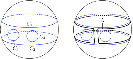
Figure 1. Four Circles and a “narrow bridge”

4.3. The Proof

We will first recall the Hopf’s maximum principle for tangential hypersurfaces in Riemannian geometry, which will be used in the proof of the Theorem 4.6. We will actually only compare hypersurfaces in $\mathbb{H}^{3}$ which are of constant mean curvature.

Lemma 4.4 ([Hop89]).

Let $S_{1}$ and $S_{2}$ be two hypersurfaces in a Riemannian manifold which intersect at a common point tangentially. If $S_{2}$ lies in positive side of $S_{1}$ around the common point, then $H_{1}\leq H_{2}$, where $H_{i}$ is the mean curvature of $S_{i}$ at the common point for $i=1,2$.

For our particular situation, we need a corollary of the maximum principle that will be used later.

Corollary 4.5.

Let $\Sigma\subset\mathbb{H}^{3}$ be a disk-type surface whose asymptotic boundary is a Jordan curve and its mean curvature is a constant $H\in(-2,2)$. Let $D$ be a totally geodesic plane in $\mathbb{H}^{3}$, and let $D(r)$ be one of the components of the boundary of $\mathscr{N}_{r}(D)$ for $r=\tanh^{-1}(|H|/2)$, then $D(r)$ is a disk-type surface with the same constant mean curvature as that of $\Sigma$, here $\mathscr{N}_{r}(D)$ denotes the $r$-neighborhood $D$. Suppose that the normal vectors on $\Sigma$ and $D(r)$ are in the same direction. If $\partial_{\infty}D\cap\partial_{\infty}\Sigma=\emptyset$, then $D(r)\cap\Sigma=\emptyset$.

Proof.

Let $\partial_{\infty}D=C$ and $\partial_{\infty}\Sigma=\Lambda$. By a Möbius transformation, we may assume that $C$ is on the horizontal plane $z=0$, i.e. $C=\{(x,y,0)\in\mathbb{R}^{3}\ |\ x^{2}+y^{2}=1\}$ and that $\Lambda$ is above the the horizontal plane $z=0$. Besides, we also assume that the normal vectors on $D(r)$ and $\Sigma$ are downward, i.e. the normal vectors point to the domains which are below the surfaces $D(r)$ and $\Sigma$ respectively.

Let $W$ be the subdomain of $\mathbb{H}^{3}$ which is below $D(r)$. Note that the surface $D(r)$ has constant principal curvature. Using the translations along the $z$-axis, we may foliate $W$ by disk-type surfaces $\{D_{t}(r)\}_{-\infty<t<0}$ whose asymptotic boundaries are circles and whose mean curvatures are the same as that of $D(r)$ with respect to the downward normal vectors. If $D(r)\cap\Sigma\neq\emptyset$, then some interior points of $\Sigma$ are contained in $W$, so from bottom to top, there is a surface $D_{t}$ touches $\Sigma$ for the first time, here $t\in(-\infty,0)$, therefore $H(D_{t}(r))>H(\Sigma)$ by the maximal principle, here $H(\cdot)$ denotes the mean curvature of the surface with respect to the downward normal vectors. This is impossible, since they are supposed to be equal. Thus $D(r)$ must be disjoint from $\Sigma$. ∎

Now we are ready to show:

Theorem 4.6.

The quasi-Fuchsian manifold $M=\mathbb{H}^{3}/\Gamma$ constructed above can not be foliated by closed surfaces of constant mean curvature.

Proof.

We will argue by contradiction and we follow the scheme outlined in the beginning of §4.1. Let us assume that our construction $M$ is foliated by surfaces of constant mean curvature, where each surface is closed and incompressible. We lift this foliation to the universal covering space $\mathbb{H}^{3}$, then we obtain a foliation of $\mathbb{H}^{3}$ such that each leaf is a disk of constant mean curvature and all disks share the same asymptotic boundary $\Lambda_{\Gamma}$. Step $(2)$: Existence of two minimal leaves $L_{t_{1}}$ and $L_{t_{2}}$.

Notice that any disk-type surface in $\mathbb{H}^{3}$ with asymptotic boundary $\Lambda_{\Gamma}$ divides $\overline{\mathbb{H}}{}^{3}$ into two parts, one of them contains $\Omega_{-}$, the other contains $\Omega_{+}$. We choose the normal vector field on the disk-type surface so that each normal vector points to the domain containing $\Omega_{-}$. Assume that there is a constant mean curvature foliation $\mathcal{F}=\{L_{t}\}$ of $\mathbb{H}^{3}$, with a parameter $t\in(-\infty,\infty)$ such that the leaves are convergent to $\Omega_{\pm}$ as $t\to{}\pm\infty$ respectively. In other words, we have

(4.3) $$\lim_{t\to\pm\infty}H(L_{t})=\pm{}2\ ,$$

where $H(L_{t})$ denotes the mean curvature of the leaf $L_{t}$ with respect to the normal vectors pointing to the domain containing $\Omega_{-}$. Here we just need to assume that $H(L_{t})$ is a continuous function of the parameter $t\in(-\infty,\infty)$.

Since $d(C_{3},C_{4})\ll{}\min\{d_{H_{0}},d_{0}\}$, there exists a minimal catenoid $\Pi_{1}$ whose asymptotic boundary is $C_{3}\cup{}C_{4}$ by Lemma 4.1. Starting from $\Omega_{-}$ to $\Omega_{+}$, there is a leaf $L_{t^{\prime}}\in\mathcal{F}$ which touches $\Pi_{1}$ for the first time, then the mean curvature of the leaf $L_{t^{\prime}}$ must be positive by the maximal principle (Lemma 4.4). Because of the limiting behavior in (4.3), there exists $t_{1}\in(-\infty,t^{\prime})$ such that the mean curvature of $L_{t_{1}}$ is zero, i.e. the leaf $L_{t_{1}}$ is a disk type minimal surface (see the left figure in Figure 2). Besides, we may choose $t_{1}$ small enough such that $H(L_{t})<0$ for all $t\in(-\infty,t_{1})$; this can be done since all leaves in $\mathcal{F}$ which are minimal must be contained in the convex hull of $\Lambda_{\Gamma}$.

Similarly, since $d(C_{1},C_{2})\ll{}d_{0}$, there exists a minimal catenoid $\Pi_{2}$ whose asymptotic boundary is $C_{1}\cup{}C_{2}$ by Lemma 4.1. Starting from $\Omega_{+}$ to $\Omega_{-}$, there exists a leaf $L_{t^{\prime\prime}}\in\mathcal{F}$ which touches $\Pi_{2}$ for the first time, then the mean curvature of the leaf $L_{t^{\prime\prime}}$ must be negative (Lemma 4.4 again). Because of the limiting behavior in (4.3), there exists $t_{2}\in(t^{\prime\prime},\infty)$ such that the mean curvature of $L_{t_{2}}$ is zero, i.e. the leaf $L_{t_{2}}$ is a disk type minimal surface (see the right figure in Figure 2). We may choose $t_{2}$ big enough such that $H(L_{t})>0$ for all $t\in(t_{2},\infty)$.

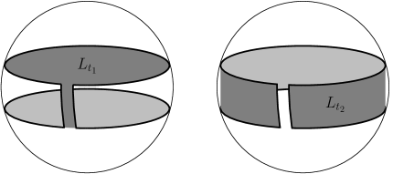
Figure 2. Two Minimal Disks

By the construction, $L_{t_{1}}\neq{}L_{t_{2}}$. Besides, $L_{t_{1}}$ is close to $\Omega_{-}$ and $L_{t_{2}}$ is close to $\Omega_{+}$, so we must have $t_{1}<t_{2}$. Note that we obtain two distinct closed minimal surfaces in the quotient manifold $M$, and hence $M$ can not be almost-Fuchsian. Step $(3)$: Some leaf $L_{t_{3}}$ must self-intersect. Let $X\subset\mathbb{H}^{3}$ be the region bounded by leaves $L_{t_{1}}$ and $L_{t_{2}}$, then by assumption $X$ is foliated by $\{L_{t}\}_{t_{1}\leq{}t\leq{}t_{2}}$, i.e.

$$X=\bigcup_{t_{1}\leq{}t\leq{}t_{2}}L_{t}\ .$$

Let

$$W_{1}=\bigcup_{-\infty<t\leq{}t_{1}}L_{t}\qquad\text{and}\qquad W_{2}=\bigcup_{t_{2}\leq{}t<\infty}L_{t}\ .$$

Clearly we have $\mathbb{H}^{3}=W_{1}\cup{}X\cup{}W_{2}$, $W_{1}\cap{}W_{2}=\emptyset$ and $X\cap{}W_{i}=L_{t_{i}}$ for $i=1,2$.

Recall that both $D_{3}$ and $D_{4}$ are totally geodesic planes, and $\partial_{\infty}D_{i}\cap\Lambda_{\Gamma}=C_{i}\cap\Lambda_{\Gamma}=\emptyset$ for $i=3,4$, so both $D_{3}$ and $D_{4}$ are disjoint from $L_{t_{2}}$ by Corollary 4.5 (In fact, $D_{i}\subset{}W_{2}$ for $i=3,4$). We choose two circles $C_{3}^{\prime}\subset{}D_{3}$ and $C_{4}^{\prime}\subset{}D_{4}$ such that $C_{3}^{\prime}$ and $C_{4}^{\prime}$ are coaxial with respect to the rotation axis of $C_{3}$ and $C_{4}$. By the Lemma 4.2, there is a compact surface $\Pi_{0}$ of constant mean curvature $-H_{0}$ with respect to the inward normal vectors, i.e., the normal vectors pointing to the domain containing the rotation axis of $C_{3}^{\prime}$ and $C_{4}^{\prime}$.

We claim that $\Pi_{0}\cap{}W_{1}=\emptyset$. Since $D_{i}\subset{}W_{2}$ for $i=3,4$, then $C_{i}^{\prime}\subset{}W_{2}$ for $i=3,4$. Therefore, if $\Pi_{0}\cap{}W_{1}\neq\emptyset$, then any point in $\Pi_{0}\cap{}W_{1}$ must be the interior point of $\Pi_{0}$. Starting from $\Omega_{-}$ to $L_{t_{1}}$, let $L_{t}$ be the leaf contained in $W_{1}$ which touches $\Pi_{0}$ for the first time, then $H(L_{t})>H_{0}$, here the normal vector at the common point points to the domain containing $\Omega_{-}$, which is the outward normal vector on $\Pi_{0}$. This is impossible since $H(L_{t})\leq{}0$ for all $t\in(-\infty,t_{1}]$.

In particular, we have $L_{t_{1}}\cap\Pi_{0}=\emptyset$ and $L_{t_{2}}\cap\Pi_{0}\neq\emptyset$. Therefore, starting from $L_{t_{1}}$ to $L_{t_{2}}$, there exists $t_{*}\in(t_{1},t_{2})$ such that the leaf $L_{t_{*}}$ touches $\Pi_{0}$ for the first time, then $H(L_{t_{*}})>H_{0}$ by the maximal principle, here the normal vector at the common point points to the domain containing $\Omega_{-}$. So there exists $t_{3}\in(t_{1},t_{*})$ such that $H(L_{t_{3}})=H_{0}$. Notice that $L_{t_{3}}$ is close to $L_{t_{1}}$, so its shape is similar to that of $L_{t_{1}}$, one may imagine that $L_{t_{3}}$ consists of two disks connected by a narrow bridge. Besides, $L_{t_{3}}$ is still contained in $X$.

We now complete the step $(3)$, namely, the leaf $L_{t_{3}}$ must self-intersect. To see this, let $D_{1}(\varepsilon)$ be the component of $\partial\mathscr{N}_{\varepsilon}(D_{1})$ that is below the geodesic plane $D_{1}$, here $\mathscr{N}_{\varepsilon}(D_{1})$ is the (hyperbolic) $\varepsilon$-neighborhood of $D_{1}$, then $D_{1}(\varepsilon)$ is a surface with constant mean curvature $H_{0}$ with respect to the upward normal vectors, i.e. the normal vectors pointing to domain not containing $C_{2}$. It is well known that the equidistant surface from a totally geodesic disk in $\mathbb{H}^{3}$ is of constant mean curvature. Similarly, let $D_{2}(\varepsilon)$ be the component of $\partial\mathscr{N}_{\varepsilon}(D_{2})$ that is above the geodesic plane $D_{2}$, then $D_{2}(\varepsilon)$ is a surface with constant mean curvature $H_{0}$ with respect to the downward normal vectors, i.e. the normal vectors pointing to domain not containing $C_{1}$. One can see $D_{1}(\varepsilon)$ as a dome below $D_{1}$, while $D_{2}(\varepsilon)$ as a dome above $D_{2}$.

Since $\partial_{\infty}D_{i}\cap\partial_{\infty}L_{t_{3}}=C_{i}\cap\Lambda_{\Gamma}=\emptyset$ for $i=1,2$, neither $D_{1}(\varepsilon)$ nor $D_{2}(\varepsilon)$ intersects $L_{t_{3}}$ by Corollary 4.5. Recall that the shape of $L_{t_{3}}$ is similar to that of $L_{t_{1}}$, i.e., $L_{t_{3}}$ consists of two disks connected by a narrow bridge. The two disks of $L_{t_{3}}$ must be below $D_{1}(\varepsilon)$ and above $D_{2}(\varepsilon)$. Recall that the (hyperbolic) distance between $D_{1}$ and $D_{2}$ is $2\varepsilon$, therefore $D_{1}(\varepsilon)\cap{}D_{2}(\varepsilon)=\{O\}$, where $O\in\mathbb{H}^{3}$ is the origin, so $L_{t_{3}}$ must self intersect. Now the theorem follows easily. ∎

References

- [AC96] James Anderson and Richard Canary, Cores of hyperbolic -manifolds and limits of Kleinian group, Amer. J. Math 118 (1996), no. 4, 745–779.
- [AMT97] Lars Andersson, Vincent Moncrief, and Anthony J. Tromba, On the global evolution problem in gravity, J. Geom. Phys. 23 (1997), no. 3-4, 191–205.
- [And83] Michael T. Anderson, Complete minimal hypersurfaces in hyperbolic -manifolds, Comment. Math. Helv. 58 (1983), no. 2, 264–290.
- [Ast94] Kari Astala, Area distortion of quasiconformal mappings, Acta Math. 173 (1994), 37–60.
- [BBZ07] Thierry Barbot, François Béguin, and Abdelghani Zeghib, Constant mean curvature foliations of globally hyperbolic spacetimes locally modelled on , Geom. Dedicata 126 (2007), 71–129.
- [BC94] Marc Burger and Richard D. Canary, A lower bound on for geometrically finite hyperbolic -manifolds, J. Reine Angew. Math. 454 (1994), 37–57.
- [Ber72] Lipman Bers, Uniformization, moduli, and Kleinian groups, Bull. London Math. Soc. 4 (1972), 257–300.
- [Bow79] Rufus Bowen, Hausdorff dimension of quasicircles, Inst. Hautes Études Sci. Publ. Math. (1979), no. 50, 11–25.
- [Bro03] Jeffery Brock, The Weil-Petersson metric and volumes of 3-dimensional hyperbolic convex cores, J. Amer. Math. Soc. 16 (2003), no. 3, 495–535.
- [Eps84] Charles L. Epstein, Envelopes of horospheres and Weingarten surfaces in hyperbolic 3-space, unpublished manuscript.
- [Eps86] by same author, The hyperbolic Gauss map and quasiconformal reflections, J. Reine Angew. Math. 372 (1986), 96–135.
- [FG85] Charles Fefferman and C. Robin Graham, Conformal invariants, Astérisque (1985), no. Numero Hors Serie, 95–116, The mathematical heritage of Élie Cartan (Lyon, 1984).
- [Geh62] F. W. Gehring, Rings and quasiconformal mappings in space, Trans. Amer. Math. Soc. 103 (1962), 353–393.
- [GHW10] Ren Guo, Zheng Huang, and Biao Wang, Quasi-Fuchsian three-manifolds and metrics on Teichmüller space, Asian J. Math. 14 (2010), no. 2, 243–256.
- [Gom87] Jonas de Miranda Gomes, Spherical surfaces with constant mean curvature in hyperbolic space, Bol. Soc. Brasil. Mat. 18 (1987), no. 2, 49–73.
- [GV73] F.W. Gehring and J. Väisälä, Holomorphic differentials and quasiconformal mappings, J. London Math. Soc. (2) 6 (1973), 504–512.
- [HL12] Zheng Huang and Marcello Lucia, Minimal immersions of closed surfaces in hyperbolic three-manifolds, Geom. Dedicata 158 (2012), 397–411.
- [Hop89] Heinz Hopf, Differential geometry in the large, Lecture Notes in Mathemtaics, vol. 1000, Springer-Verlag, Berlin, 1989.
- [KS07] Kirill Krasnov and Jean-Marc Schlenker, Minimal surfaces and particles in 3-manifolds, Geom. Dedicata 126 (2007), 187–254.
- [KS08] by same author, On the renormalized volume of hyperbolic 3-manifolds, Com. Math. Phy. 279 (2008), no. 3, 637–668.
- [Lóp00] Rafael López, Hypersurfaces with constant mean curvature in hyperbolic space, Hokkaido Math. J. 29 (2000), no. 2, 229–245.
- [LV73] O. Lehto and K. I. Virtanen, Quasiconformal mappings in the plane, second ed., Springer-Verlag, New York, 1973.
- [Mar74] Albert Marden, The geometry of finitely generated kleinian groups, Ann. of Math. (2) 99 (1974), 383–462.
- [Mes07] Geoffrey Mess, Lorentz spacetimes of constant curvature, Geom. Dedicata 126 (2007), 3–45.
- [Mos68] G. D. Mostow, Quasi-conformal mappings in -space and the rigidity of hyperbolic space forms, Inst. Hautes Études Sci. Publ. Math. (1968), no. 34, 53–104.
- [MP07] Rafe Mazzeo and Frank Pacard, Constant curvature foliations on asymptotically hyperbolic spaces, Preprint, arxiv.org/math.DG/0710.2298 (2007).
- [MT98] K. Matsuzaki and M. Taniguchi, Hyperbolic manifolds and Kleinian groups, Oxford Mathematical Monographs, The Oxford University Press, New York, 1998.
- [Pal99] Oscar Palmas, Complete rotation hypersurfaces with constant in space forms, Bol. Soc. Brasil. Mat. (N.S.) 30 (1999), no. 2, 139–161.
- [PP01] S. J. Patterson and Peter A. Perry, The divisor of Selberg’s zeta function for Kleinian groups, Duke Math. J. 106 (2001), no. 2, 321–390, Appendix A by Charles Epstein.
- [Rub05] J. Hyam Rubinstein, Minimal surfaces in geometric 3-manifolds, Global theory of minimal surfaces, Clay Math. Proc., vol. 2, Amer. Math. Soc., Providence, RI, 2005, pp. 725–746.
- [Smi10] Stanislav Smirnov, Dimension of quasicircles, Acta Math. 205 (2010), no. 1, 189–197.
- [SU82] J. Sacks and K. Uhlenbeck, Minimal immersions of closed Riemann surfaces, Trans. Amer. Math. Soc. 271 (1982), no. 2, 639–652.
- [Sul87] Dennis Sullivan, Related aspects of positivity in Riemannian geometry, J. Differential Geom. 25 (1987), no. 3, 327–351.
- [SY79] Richard Schoen and Shing-Tung Yau, Existence of incompressible minimal surfaces and the topology of three-dimensional manifolds with nonnegative scalar curvature, Ann. of Math. (2) 110 (1979), no. 1, 127–142.
- [Tau04] Clifford Henry Taubes, Minimal surfaces in germs of hyperbolic 3-manifolds, Proceedings of the Casson Fest, Geom. Topol. Monogr., vol. 7, Geom. Topol. Publ., Coventry, 2004, pp. 69–100 (electronic).
- [Thu82] William P. Thurston, The geometry and topology of three-manifolds, 1982, Princeton University Lecture Notes.
- [Uhl83] Karen K. Uhlenbeck, Closed minimal surfaces in hyperbolic -manifolds, Seminar on minimal submanifolds, Ann. of Math. Stud., vol. 103, Princeton Univ. Press, Princeton, NJ, 1983, pp. 147–168.
- [Wan12] Biao Wang, Minimal surfaces in quasi-Fuchsian -manifolds, Math. Ann. 354 (2012), 955–966.