Scalable Probabilistic Similarity Ranking in Uncertain Databases (Technical Report)

Abstract

This paper introduces a scalable approach for probabilistic top-k similarity ranking on uncertain vector data. Each uncertain object is represented by a set of vector instances that are assumed to be mutually-exclusive. The objective is to rank the uncertain data according to their distance to a reference object. We propose a framework that incrementally computes for each object instance and ranking position, the probability of the object falling at that ranking position. The resulting rank probability distribution can serve as input for several state-of-the-art probabilistic ranking models. Existing approaches compute this probability distribution by applying a dynamic programming approach of quadratic complexity. In this paper we theoretically as well as experimentally show that our framework reduces this to a linear-time complexity while having the same memory requirements, facilitated by incremental accessing of the uncertain vector instances in increasing order of their distance to the reference object. Furthermore, we show how the output of our method can be used to apply probabilistic top-k ranking for the objects, according to different state-of-the-art definitions. We conduct an experimental evaluation on synthetic and real data, which demonstrates the efficiency of our approach.

I Introduction

In the past two decades, there has been a great deal of interest in developing efficient and effective methods for similarity queries in spatial, temporal, multimedia and sensor databases. Similarity ranking is a hot topic in database research because a large number of emerging applications require exploratory querying on the aforementioned databases. A ranking query orders the objects in a database with respect to their similarity to a reference object. In a spatial database context, nearest neighbor queries rank the contents of a spatial object set (e.g., restaurants) in increasing order of their distance to a reference location. In a database of images, a similarity query ranks the feature vectors of images in increasing order of their distance (i.e., dissimilarity) to a query image.

More recently, it has been recognized that many applications dealing with spatial, temporal, multimedia, and sensor data have to cope with uncertain or imprecise data. For instance, in the spatial domain, the locations of objects usually change continuously, thus the positions tracked by GPS devices are often imprecise. Similarly, vectors of values collected in sensor networks (e.g., temperature, humidity, etc.) are usually inaccurate, due to errors in the sensing devices or time delays in the transmission. Finally, images collected by cameras may have errors, due to low-resolution or noise. As a consequence, there is a need to adapt storage models and indexing/search techniques to deal with uncertainty. There is already a volume of research on probabilistic data models [3, 19, 20, 2].

In this paper, we focus on similarity ranking of uncertain vector data. Prior work in this direction includes [7, 9, 23, 6, 14, 15, 10, 21]. In a nutshell, there are two models for capturing uncertainty of objects in a high dimensional space. In the continuous uncertainty model, the uncertain values of an object are represented by a continuous probability distribution function (pdf) within the vector space. This type of representation is often used in applications where the uncertain values are assumed to follow a specific probability density function (pdf), e.g. a Gaussian distribution [6]. Similarity search methods based on this model involve expensive integrations of the pdf’s, thus special approximation techniques for efficient query processing are typically employed [23]. In the discrete uncertainty model, each object is represented by a discrete set of alternative values, and each value is associated with a probability [14]. The main motivation of this representation is that, in most real applications, data are collected in a discrete form (e.g., information derived from sensor devices). In this paper, we adopt the discrete uncertainty model which also complies with the x-relations model used in the Trio system [1].

Consider, for example, a set of three two-dimensional objects $A$, $B$, and $C$ (e.g., locations of mobile users), and their corresponding uncertain instances $\{a_{1},a_{2}\}$, $\{b_{1},b_{2},b_{3}\}$, and $\{c_{1},c_{2},c_{3}\}$, as shown in Figure 1(a). Each instance carries a probability (shown in brackets) and instances of the same object are mutually-exclusive. In addition, the sum of probabilities of each object’s instances cannot exceed 1. Assume that we wish to rank the objects $A$, $B$, and $C$ according to their distances to the query point $q$ shown in the figure. Clearly, several rankings are possible. In specific, each combination of object instances defines an order. For example, for combination $\{a_{1},b_{1},c_{1}\}$ the object ranking is $(B,A,C)$ while for combination $\{a_{2},b_{3},c_{1}\}$ the object ranking is $(A,B,C)$. Each combination corresponds to a possible world [1], whose probability can be computed by multiplying the probabilities of the instances that comprise it, assuming independent existence probabilities between the instances of different objects.

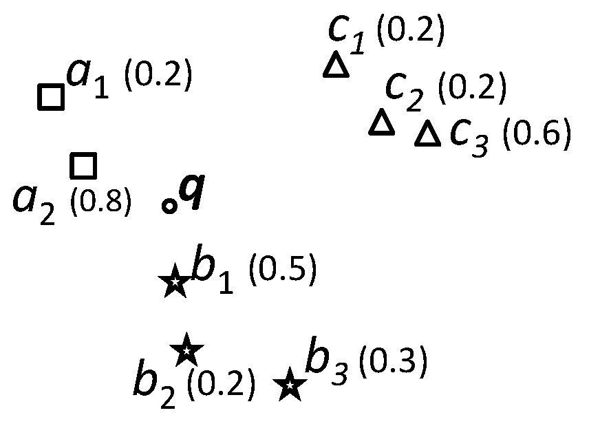
(a) Object Instances

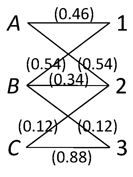
(b) Bipartite Graph

Figure 1: Object Instances and Rank Probability Graph

The example illustrates the ambiguity of ranking in uncertain data. On the other hand, most applications require the definition of a non-ambigous object ranking. For example, assume that a robbery took place at location $q$ and the objects correspond to the positions of suspects that are sampled around the time that the robbery took place. The probabilities of the samples depend on various factors (e.g., time-difference of the sample to the robbery event, errors of capturing devices, etc.). As an application, we may want to define a definite probabilistic proximity ordering of the suspects to the event, in order to prioritize interrogations.

Various top-$k$ query approaches have been proposed generating un-ambiguous rankings from probabilistic data. Examples are U-top$k$ [22], U-$k$Ranks [22], PT-$k$ [13], Global top-$k$ [28], and expected rank [10]. A summary of these ranking models can be found in [10]. All of them attempt to weigh the objects based on their probability to be in each of the first $k$ ranks, but they use different ways to define the weights.

A common module in most of these approaches is the computation for each object instance $x$ the probability $P_{i}$ that $i$ objects are closer to $q$ than $x$ for all $1\leq i\leq k$. The resulting probabilities are aggregated to build the probability of each object at each rank. For example, the U-$k$Ranks query reports the $i^{th}$ result as the object that is the most likely to be ranked $i^{th}$ over all possible worlds. For this computation, we obviously need the probabilities of all instances to be ranked $i^{th}$ over all possible worlds. The probability that an object is ranked at a specific position $i$ can be computed by summing the probabilities of the possible worlds that support this occurrence. In our example, the probability that object $A$ occurs as first one is 0.46 and the probability that object $B$ is the first is 0.54. All possible occurrences and the corresponding probabilities are represented by the object-rank bipartite graph which is shown in Figure 1(b). Non-existing edges imply zero probability, i.e. it is not possible that the object occurs at the corresponding ranking position. In this example, all instances of $A$ precede all those of $C$, so $C$ cannot occur as first object and $A$ cannot be ranked to the last position.

In this paper, we propose a framework that, given a database with uncertain vector objects, computes the rank probabilities of the object instances (e.g., $a_{1}$) in linear time to the total number of instances of all objects. — assuming that the instances are accessed in increasing distance order to the query object $q$ (e.g., with the help of a nearest neighbor search algorithm [12]). As these can be aggregated on-the-fly, our framework also computes the rank probabilities of the objects (e.g., $A$) at the same cost. This is a great improvement, over the state-of-the-art [26], which computes these probabilities in quadratic time.

I-A Problem Definition

Analogously to the Trio [1] system, we define an uncertain database as a set of uncertain objects (x-tuples), each including a number of alternatives associated with probabilities. Here, we consider uncertain vector objects in a $d$-dimensional vector space, i.e., each object is assigned to multiple alternative positions associated with a probability value. Let us note that this model assumes independence among the uncertain objects.

Definition 1 (Uncertain Vector Objects)

An uncertain vector object $o$ corresponds to a finite set of alternative points in a $d$-dimensional vector space, called object instances, each associated with a probability value, i.e., $o=\{(x,p)$, where $x\in\mathbb{R}^{d}$, and $p\in[0,1]\}$ is the probability that $o$ has position $x$. The probabilities of the object instances represent a discrete probability distribution of the alternative points, such that the condition $\sum_{(x,p)\in o}p\leq 1$ holds. The collection of instances of all objects forms the uncertain database $\mathcal{D}$.

Note that the condition $\sum_{(x,p)\in o}p<1$ implies existential uncertainty, meaning that the object may not exist at all. We assume that the database objects are already given in the discrete representation as specified above. In case of an uncertain database where the uncertain objects are represented by a continuous probability function (pdf), the generally applicable concept of sampling can be used to transform the objects to the discrete representation as defined above.

Given a database of uncertain vector objects, our goal is to compute for each object instance and for the first $k$ rank positions, the probability of the object to be in that position.

Definition 2 (Rank Probability)

Given a query point $q$, an instance $x\in\mathcal{D}$, belonging to object $o$, and a rank $i\in\{1,\dots,k\}$, the probabilistic rank $p\_rank_{q}:(\mathcal{D}\times\{1,\dots,k\})\rightarrow[0,1]$ reports how likely $(i-1)$ objects $o^{\prime}\neq o$ are closer to $q$ than $x$, i.e., the probability that $x$ is at the $i^{th}$ ranking position according to the distance (i.e., dissimilarity) between $x$ and $q$.

Since the number of possible worlds is exponential in the number of uncertain objects, it is impractical to enumerate all of them in order to find the rank probabilities of all object instances. Recently, it has been shown in [25] that we can compute the probabilities between all object instances and ranks in $O(kn^{2})$ time, where $n$ is the number of object instances required to be accessed until the solution is confirmed. This solution can be applied to all problems that comply to the x-relation model (including our problem). In this paper, we propose a significant improvement of this approach, which reduces the time complexity to $O(kn)$.

In Section V, we discuss in detail how our method can be used as a module in various models that rank the objects according to the rank probabilities of their instances.

Although in the paper, we focus on databases of uncertain objects as in Definition 1, our results apply in general to x-relations as defined in [1], which model mutual-exclusiveness constraints between existentially uncertain tuples (i.e., object instances in our model). Thus, our method is general and it can be used irrespectively to whether we have uncertain objects or existentially uncertain tuples with exclusiveness constraints, expressed by x-tuples.

I-B Contributions and Outline

The main contributions of this paper can be summarized as follows:

• We propose a framework based on iterative distance browsing that efficiently supports probabilistic similarity ranking in uncertain vector databases.

• We present a novel and theoretically founded approach for computing the rank probabilities of each object. We prove that our method reduces the computational cost of the rank probabilities from O($kn^{2}$), achieved by the best currently known method, to O($kn$).

• We show how diverse state-of-the-art probabilistic ranking models can use our framework to accelerate computation.

• We conduct an experimental evaluation, using real and synthetic data, which demonstrates the applicability of our framework and verifies our theoretical findings.

The rest of the paper is organized as follows: In the next section, we survey existing work in the field of managing and querying uncertain data. In Section III, we introduce our framework for computing the rank probabilities of uncertain object instances, followed by the details regarding the efficient incremental rank probability computation for each object instance.

The complete algorithm for computing the rank probabilities for all instances and the corresponding objects is presented in Section IV. We experimentally evaluate the efficiency of our approach in Section VI and conclude the paper in Section VII.

II Related Work

The potential of uncertain data processing has achieved increasing interest in diverse application fields, e.g., sensor monitoring [8], traffic analysis and location-based services [24], etc.

By now, uncertain data management has been established as an important branch of research within the database community, with increasing tendency. Existing approaches in this field of modelling of, managing of and query processing on uncertain data can be categorized into diverse directions, including probabilistic databases [3, 19, 20, 2], indexing of uncertain data [9, 23, 6] and probabilistic query processing [7, 11, 6, 14, 5, 26, 22].

Probabilistic databases usually relate to probabilistic relational data, i.e. relations with uncertain tuples [11], and use the possible worlds semantic [2] which is a probability distribution on all possible database instances; a database instance corresponds to a subset of uncertain tuples. In the general model, the possible worlds are constrained by rules that are defined on the tuples in order to incorporate object (tuple) correlations [20]. The ULDB model proposed in [3] and used in the Trio [1] system supports uncertain tuples with alternative instances which are called x-tuples. Relations in ULDB are called x-relations containing a set of x-tuples. Each x-tuple corresponds to a set of tuple instances which are assumed to be mutually exclusive, i.e. no more than one instance of an x-tuple can appear in a possible world instance at the same time. This probabilistic data model closes the gap between two prevalent uncertainty models, the tuple uncertainty [11] and the attribute uncertainty [7]. An x-tuple is able to model an object with attribute value uncertainty; i.e., the instances of an x-tuple represent the probability value distribution of the corresponding uncertain attribute.

In this paper, we adopt this concept to model uncertain vector objects. An uncertain vector object would correspond to an x-tuple of alternative uncertain instances of the object. Several approaches for indexing uncertain vector objects have been proposed [9, 23, 6, 27]. They mainly differ in the uncertainty model supported and in the type of supported similarity queries. In [6], the Gauss-tree is introduced, which is an index for managing large amounts of uncertain objects with their uncertain attribute represented by a Gaussian distribution function. The proposed system aims at efficiently answering identification queries like “Give me all persons in the database that could be shown on a given image with a probability of at least 10%”. Additionally, [6] proposed probabilistic identification queries which are based on a Bayesian setting. Later, in [6] an approach for incrementally retrieving the $k$ most likely uncertain objects that might be placed in a given query interval is proposed. Note that this definition is sematically different than the problem studied in this paper.

In [6], objects which have the highest probability of being located inside a given query range are reported. In contrast, the approaches for managing uncertain vector objects proposed in [7, 9, 23] support arbitrarily shaped probability distribution functions for uncertain object attributes. Similar to [6], the approaches in [9, 23] focus on probability computations based on query predicates according to a given query range and, thus, are not applicable for our problem. Although [27] studies probabilistic ranking of objects according to their distance from a reference query point, the solutions are limited to existentially uncertain spatial data with a single alternative.

We can categorize existing probabilistic querying approaches according to the uncertainty model they use. While probabilistic similarity queries over uncertain vector data are dedicated to the attribute value uncertainty model [7, 14], probabilistic top-$k$ query approaches are usually associated with tuple uncertainty data in probabilistic databases [22, 25, 19, 26]. There exists a third probabilistic query category concerning spatially extended uncertain data as proposed in [18]. But there is only little work in this direction.

To the best of our knowledge, only [5] addresses probabilistic ranking according to our problem definition. There, a divide and conquer method for accelerating the computation of the ranking probabilities is proposed. Although the proposed approach achieves a significant speed-up compared to the naive solution incorporating each possible database instance, its runtime is still exponential. Related to our ranking problem, significant work has been done in the field of probabilistic top-$k$ query processing. Soliman et al. [22] were the first who studied such problems on the x-relations model of [3]. They proposed two ways of ranking uncertain tuples. In the first, uncertain top-$k$ (U-Top$k$) query, the objective is to find the $k$-permutation of the most likely tuples to be the top-$k$. In our setting, this corresponds to finding the top-$k$ most probable object instances (belonging to different objects) in all possible worlds. The uncertain $k$-ranks query (U-$k$Ranks) reports a probabilistic ranking of the tuples (again, not the x-tuples). However, an efficient approach for this problem is only given for the case where the tuples are mutually independent which does not hold for the x-relation model. At the same time Re et al. proposed in [19] an efficient but approximative probabilistic ranking based on the concept of Monte-Carlo simulation. Later, Yi et al. proposed in [26] the first efficient exact probabilistic ranking approach for the x-relation model, for both cases of single-alternative x-tuples only, i.e. x-tuples with only one uncertain instance, and multi-alternative x-tuples. They proposed dynamic programming based methods for the computation of uncertain ranking queries, which have much lower costs than the previously best known results. Furthermore, they proposed early stopping conditions for accessing the tuples. Their methods for U-Top$k$ and U-$k$Ranks queries have O($nlogk$) and O($kn^{2}$) time complexity, respectively. The cost of the U-$k$Ranks algorithm is dominated by the computation of the probability of each accessed tuple to be in each of the $k$ first ranks. In this paper, we also use this as a module of finding the object-rank probabilities. However, we propose an improvement of their O($kn^{2}$) algorithm that does the same work in O($kn$) without increasing the memory requirements.

In a recent paper, Cormode et al. [10] reviewed alternative top-$k$ ranking approaches for uncertain data, including the U-Top$k$ and U-$k$Ranks queries, and argued for a more robust definition of ranking, namely the expected rank for each tuple (or x-tuple). This is defined by the weighted sum of the ranks of the tuple in all possible worlds, where each world in the sum is weighed by its probability. The $k$ tuples with the lowest expected ranks are argued to be a more appropriate definition of a top-$k$ query than previous approaches. Nevertheless, we found by experimentation that such a definition may not be appropriate for ranking objects (i.e., x-tuples), whose instances have large variance (i.e., they are scattered far from each other in space). In general, the result of this ranking method is similar to the brute-force approach that would take the mean of the instances for each object and rank these means. On the other hand, approaches that take into consideration the rank probabilities (e.g., U-$k$Ranks) would be more suitable for such data. This is the reason why we focus on the computation of rank probabilities in this paper. Another piece of recent related work is [21], where the goal is to rank uncertain objects (i.e., x-tuples) whose score is uncertain and can be described by a range of values. Based on these ranges, the authors define a graph that captures the partial orders among objects. This graph is then processed to compute U-$k$Ranks and other queries. Although this work has similar objectives to ours, it operates on a different input, where the distribution of uncertain scores is already known, as opposed to our work which dynamically computes this distribution by performing a linear scan over the ordered object instances.

III Probabilistic Ranking Framework

Our framework basically consists of two modules which are performed in an iterative way:

• The first module (distance browsing) incrementally retrieves the instances of all objects in order of their distance to $q$. This can be achieved with the help of a multi-dimensional index (e.g., an $R^{*}$-tree index [16]), using an incremental nearest neighbor search algorithm [12].

• The second module computes the probabilistic ranks $p\_rank_{q}(o_{j},i)$ of each object instance $o_{j}$ reported from the distance browsing for all $1\leq i\leq k$. This step is the main focus of this paper, because of its potentially high computational cost. A naive solution would take into account all possible worlds that include the instance and update the probabilities accordingly, however, as discussed before, there already exists an efficient solution which can perform this computation in quadratic time and linear space [25]. In this paper, we improve this method to a linear time and space complexity algorithm. The key idea is to use the probabilistic ranks of the previous object instance to derive those of the currently accessed one in O($k$) time. Section III-B has the details of this improvement.

Our framework is illustrated in Figure 2. The computation of the probability distributions is iteratively processed within a loop. First, we initialize a distance browsing among the object instances starting from a given query point $q$. For each object instance fetched from the distance browsing (Module 1), we compute the corresponding rank probabilities (Module 2) and update the rank probability distributions generated from the probabilistic ranking routine.

Note that the rank probabilities of the object instances (i.e., tuples in the x-relations model) reported from the second module can be optionally aggregated into rank probabilities of the objects (i.e., x-tuples in the x-relations model). The probability that an uncertain vector object $o=\{(x_{1},p_{1}),\ldots,(x_{s},p_{s})\}$ is at the $i^{th}$ ranking position according to the distance between $o$ and a reference query object $q$ is

$$p\_rank_{q}(o,i)=\sum_{l=1,\ldots,s}p_{l}\cdot p\_rank_{q}(x_{l},i).$$

Our framework can be used to compute the object-based rank probabilities by maintaining a list of objects from which instances have been seen so far and successively aggregate the rank probabilities by means of the instance-based rank probabilities reported from the framework.

Finally, in a postprocessing step, the rank probability distributions computed by our framework can be used to generate a definite ranking of the objects or object instances. The objective is to find a non-ambiguous ranking where each object or object instance is uniquely assigned to one rank. Here, one can plug-in any user-defined ranking method that requires rank probability distributions of objects in order to compute unique positions. In Section V, we illustrate this for several well-known probabilistic ranking queries that make use of such distributions. In particular, we demonstrate that by using our framework we can process such queries in O($nlogn+k\cdot n$) time, as opposed to existing approaches that require O($k\cdot n^{2}$) time.

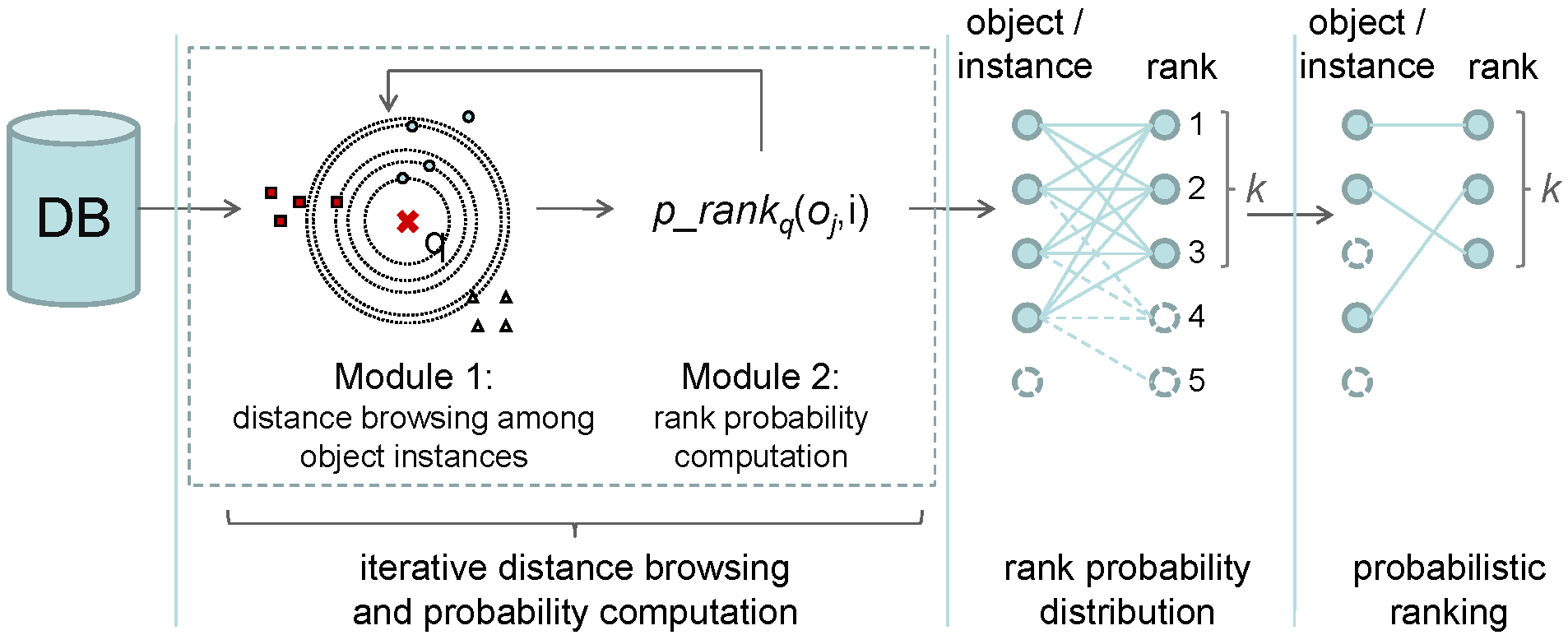
Figure 2: Framework for probabilistic similarity ranking.

Table of Notations
$\mathcal{D}$	an uncertain database
$N$	the cardinality of $\mathcal{D}$
$q$	a query vector in respect to which a probabilistic ranking is computed
$k$	the ranking depth that determines the number of ranking positions of the ranking query result
$D$	a distance browsing of $\mathcal{D}$ with respect to $q$
$o$	an uncertain vector object corresponding to a finite set of alternative vector point instances
$x$,$y$	vector point instances
$o_{X},o_{Y}$	the objects that the instances $x$ and $y$ respectively belong to
$p$	the probability that an uncertain vector object matches a given vector position
$P_{i}(o)$	the probability that object $o$ is assigned to the $i$-th ranking position $i$, i.e. the probability that exactly ($i$-1) objects in $(\mathcal{D}\setminus\{o\})$ are closer to $q$ than $o$
$\hat{P}_{i}(x)$	the probability that an instance $x$ of object $o$ is assigned to the $i$-th ranking position $i$, i.e. the probability that exactly $i-1$ objects in $(\mathcal{D}\setminus\{o\})$ are closer to $q$ than $x$
$AOL$	Active Object List
$\mathcal{S}$	a set of objects that have already been seen, i.e. the set that contains an object $o$ iff at least one instance of $o$ has already been returned by the distance browsing $D$
$\mathcal{S}^{o}$	a set that contains the objects that have already been seen, except for object $o$, i.e. $\mathcal{S}^{o}=\mathcal{S}\setminus\{o\}$
$P_{i,S,x}$	the probability that exactly $i$ objects $o$ $\in S$ are closer to $q$ than an object instance $x$
$P_{x}(o)$	the probability that object $o$ is closer to query point $q$ than the vector point $x$; computable using Lemma 1

TABLE I: Table of notations used in this work.

III-A Dynamic Probability Computation

Consider an uncertain object $o$, defined by $m$ probabilistic instances $o=\{(x_{1},p_{1}),\dots,(x_{m},p_{m})\}$. The probability that $o$ is assigned to a given ranking position $i$ is equal to the chance that exactly $i-1$ objects $o^{\prime}\in(\mathcal{D}\setminus o)$ are closer to the query object $q$ than the object $o$. This can be computed by aggregating the probabilities over all instances $(x,p)$ of $o$ that exactly $i-1$ objects $o^{\prime}$ are closer to $q$ than the instance $(x,p)$. Formally,

$$P_{i}(o)=\sum_{(x,p)\in o}\hat{P}_{i}(x|(o=x))$$

where $P_{i}(o)$ denotes the probability that o is assigned to the ranking position $i$, i.e., exactly $i-1$ objects in $(\mathcal{D}\setminus o)$ are closer to $q$ than $o$. The conditional probability $\hat{P}_{i}(x|(o=x))$ denotes the probability that exactly $i-1$ objects in $(\mathcal{D}\setminus o)$ are closer to $q$ than the object instance $x$ of $o$, given that the object $o$ is in fact at the location instance $x$. Since the conditional probability $\hat{P}_{i}(x|(o=x))$ only depends on the objects $o^{\prime}\in(\mathcal{D}\setminus o)$ and is thus independent of $o$, we obtain:

$$P_{i}(o)=\sum_{(x,p)\in o}(\hat{P}_{i}(x)\cdot P(o=x))=\sum_{(x,p)\in o}(\hat{P}_{i}(x)\cdot p)$$ (1)

Based on the above formula we can compute the probabilities for an object $o$ to be assigned to each of the ranking positions $i\in\{1,\dots,k\}$ by computing the probabilities $P_{i}(x)$ for all instances $(x,p)$ of $o$. As mentioned above, we perform this computation in an iterative way, i.e., whenever we fetch a new object instance $(x,p)$ we compute all probabilities $\hat{P}_{i}(x)\cdot p$ for all $i\in\{1,\ldots,k\}$. Thereby, in a list we store the current probability state according to all ranking positions $i\in\{1,\ldots,k\}$ for each object for which we already have accessed some instances and for which we expect to obtain further instances in the remaining iterations. Whenever the probabilities according to a new object instance are computed, we update the list by adding the new probabilities to the current probability state.

In the following, we show how to compute the probabilities $\hat{P}_{i}(x)\cdot p$ for all $i\in\{1,\ldots,k\}$ for a given object instance $(x,p)$ of an uncertain object $o$ which is assumed to be currently fetched from the distance browsing (Step 1). For this computation we first need, for all uncertain objects $o^{\prime}\in\mathcal{D}$, the probability $P_{x}(o^{\prime})$ that $o^{\prime}$ is closer to $q$ than the current object instance $x$. These probabilities are stored in an Active Object List $AOL$, which can easily be kept updated due to the following obvious lemma:

Lemma 1

Let $q$ be the query object and $(x,p)$ be the object instance of an object $o$ fetched from the distance browsing in the current processing iteration. The probability that an object $o^{\prime}\neq o$ is closer to $q$ than $x$ is

$$P_{x}(o^{\prime})=\sum_{(x^{\prime},p^{\prime})\in o^{\prime}}p^{\prime}\mathrm{,}$$

where (x’,p’) are the instances fetched in previous processing iterations.

Lemma 1 says that we can accumulate in overall linear space the sums of probabilities of all instances for each object, which have been seen so far and use them to compute $P_{x}(o^{\prime})$ given the current instance $x$ and any object $o^{\prime}$ in $\mathcal{D}$. In fact, we only need to manage in the list the probabilities of those objects for which we already have accessed an instance and for which we expect to access further instances in the remaining iterations.

Now let us see how we can use list $AOL$ to efficiently compute the probabilities $\hat{P}_{i}(x)$. Assume that $(x,p)\in o$ is the current object instance reported from distance browsing. Let $\mathcal{S}=\{o_{1},\ldots,o_{j}\}$ be the set of objects which have been seen so far, i.e. for which we already have seen at least one object instance. We use the same observation as in [25]. The probability that an object $o\in\mathcal{S}$ appears at ranking position $i$ of the first $j$ objects seen so far only depends on the event that $i-1$ of the remaining $j-1$ objects $p\in\mathcal{S}$ ($p\neq o$) appear before $o$, no matter which of these objects fulfill this criterion. Let $\mathcal{S}^{o}$ denote the set of objects seen so far without object $o$, i.e. $\mathcal{S}^{o}=\mathcal{S}\setminus\{o\}$. Furthermore, let $P_{i,\mathcal{S}^{o},x}$ denote the probability that exactly $i$ objects of $\mathcal{S}^{o}$ are closer to $q$ than the object instance $x$. Now, we can formulate the recursive function:

$$P_{i,\mathcal{S}^{o},x}=P_{i-1,\mathcal{S}^{o}\setminus\{o^{\prime}\},x}\cdot P_{x}(o^{\prime})+P_{i,\mathcal{S}^{o}\setminus\{o^{\prime}\},x}\cdot(1-P_{x}(o^{\prime}))\mathrm{,}$$

where

$$P_{0,\emptyset,x}=1\mbox{ and }P_{i,\mathcal{S}^{o},x}=0\mbox{, iff }i>|\mathcal{S}^{o}|\vee i<0.$$ (2)

The correctness of Equation 2 can be shown by the following intuition: the event that $i$ objects of $\mathcal{S}^{o}$ are closer to $q$ than $x$ occurs if one of the following conditions holds. In the case that an object $o^{\prime}\in\mathcal{S}^{o}$ is closer to $q$ than $x$, then $i-1$ objects of $\mathcal{S}^{o}\setminus\{o^{\prime}\}$ must be closer to $q$. Otherwise, if we assume that object $o^{\prime}\in\mathcal{S}^{o}$ is farther to $q$ than $x$, then $i$ objects of $\mathcal{S}^{o}\setminus\{o^{\prime}\}$ must be closer to $q$.

For each object instance $(x,p)$ reported from the distance browsing, we have to apply the recursive function as defined above.

Specifically, we have to compute for each instance $(x,p)$ the probabilities $P_{i,\mathcal{S}^{o},x}$ for all $i\in\{0,\ldots,\min\{k,|\mathcal{S}^{o}|\}\}$ and for $j=|\mathcal{S}^{o}|$ subsets of $\mathcal{S}^{o}$. If $n=|\mathcal{D}|$, this has a cost factor of O($k\cdot n$) per object instance retrieved from the distance browsing, leading to a total cost of O($k\cdot n^{2}$). Assuming that $k$ is a small constant, we have an overall runtime of O($n^{2}$).

In the following, we show how we can compute each $P_{i,\mathcal{S}^{o},x}$ in constant time by utilizing the probabilities computed for the previously accessed instance.

III-B Incremental Probability Computation

Let $(x,p_{x})\in o_{X}$ and $(y,p_{y})\in o_{Y}$ be two object instances consecutively returned from the distance browsing. W.l.o.g. let $(x,p_{x})$ be returned before $(y,p_{y})$. Each of the probabilities $P_{i,\mathcal{S}^{o_{Y}},y}$ ($i\in\{0,\ldots,|\mathcal{S}^{o_{Y}}|\}$) can be computed from the probabilities $P_{i,\mathcal{S}^{o_{X}},x}$ in constant time. In fact, the probabilities $P_{i,\mathcal{S}^{o_{Y}},y}$ can be computed by considering at most one recursion step backward.

The following three cases have to be considered. The first two are easy to tackle and the third one is the most common and challenging one.

Case 1: Both instances belong to the same object, i.e. $o_{X}=o_{Y}$.

Case 2: Both instances belong to different objects, i.e. $o_{X}\neq o_{Y}$ and $(y,p_{y})$ is the first returned instance of object $o_{Y}$.

Case 3: Both instances belong to different objects, i.e. $o_{X}\neq o_{Y}$ and $(y,p_{y})$ is not the first returned instance of object $o_{Y}$.

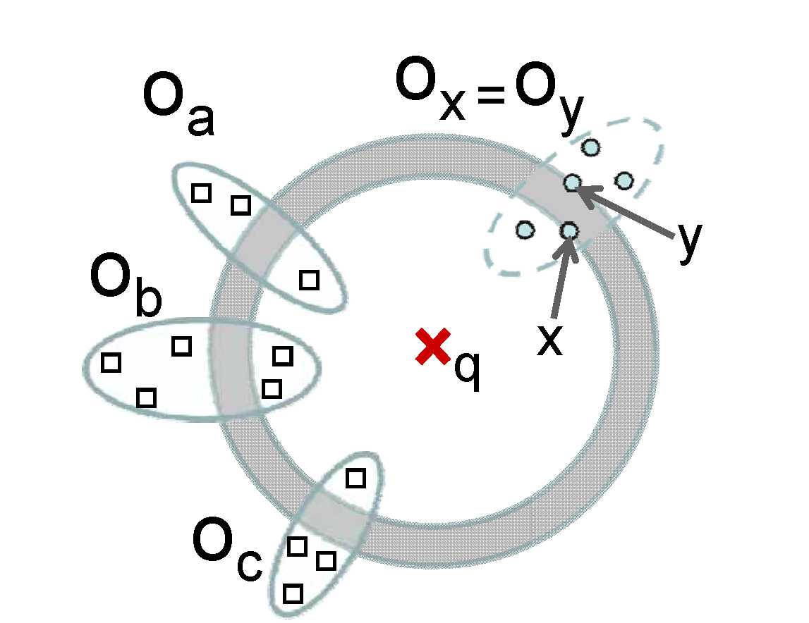
(a) Case 1: Instances $(x,p_{x})$ and $(y,p_{y})$ belong to the same object.

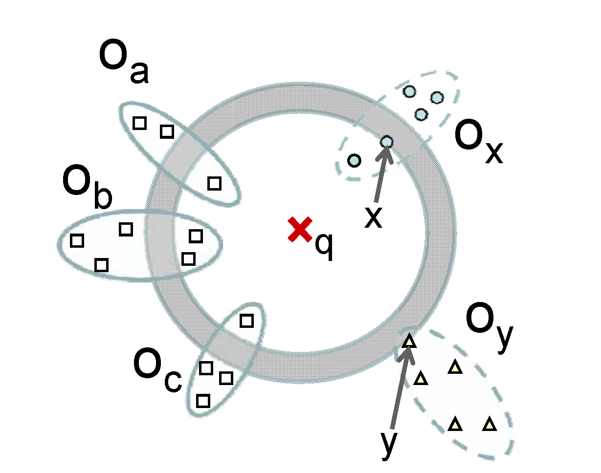
(b) Case 2: Instance $(y,p_{y})$ is the first returned instance of object $o_{Y}$.

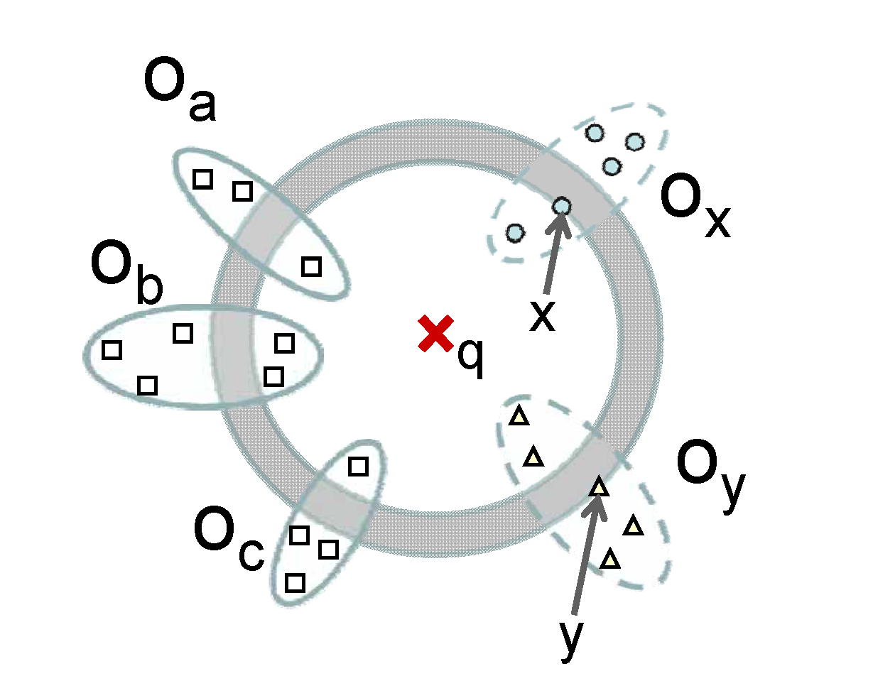
(c) Case 3: Instance $(y,p_{y})$ is not the first returned instance of object $o_{Y}$.

Figure 3: Cases to be considered when updating the probabilities, assuming $x$ was the last processed instance and $y$ is the current one.

Now, we show how the probabilities $P_{i,\mathcal{S}^{o_{Y}},y}$ for $i\in\{0,\ldots,|\mathcal{S}^{o_{Y}}|\}$ can be computed in constant time considering the above cases which are illustrated in Figure 3.

In the first case (cf. Figure 3(a)), the probabilities $P_{x}(o)$ and $P_{y}(o)$ of all objects in $o\in\mathcal{S}^{o_{X}}$ are equal, because the instances of objects in $\mathcal{S}^{o_{X}}$ that appear within the distance range of $q$ of $y$ and within the distance range of $x$ are identical. Since the probabilities $P_{i,\mathcal{S}^{o_{Y}},y}$ and $P_{i,\mathcal{S}^{o_{X}},x}$ only depend on the $P_{x}(o)$ for all objects $o\in\mathcal{S}^{o_{X}}$, it is obvious that $P_{i,\mathcal{S}^{o_{Y}},y}=P_{i,\mathcal{S}^{o_{X}},x}$ for all $i$.

In the second case (cf. Figure 3(b)) we can exploit the fact that $P_{i,\mathcal{S}^{o_{X}},x}$ does not depend on $o_{Y}$. Thus, given the probabilities $P_{i,\mathcal{S}^{o_{X}},x}$, we can easily compute the probability $P_{i,\mathcal{S}^{o_{Y}},y}$ by incorporating the object $o_{X}$ using the recursive Equation 2:

$$P_{i,\mathcal{S}^{o_{Y}},y}=$$

$$P_{i-1,\mathcal{S}^{o_{Y}}\setminus\{o_{X}\},y}\cdot P_{y}(o_{X})+P_{i,\mathcal{S}^{o_{Y}}\setminus\{o_{X}\},y}\cdot(1-P_{y}(o_{X})).$$

Since $\mathcal{S}^{o_{Y}}\setminus\{o_{X}\}=\mathcal{S}^{o_{X}}\setminus\{o_{Y}\}=\mathcal{S}-\{o_{X},o_{Y}\}$ holds by definition and no instance of any object in $\mathcal{S}^{o_{X}}\setminus\{o_{Y}\}$ appears within the distance range of $q$ according to $y$ but not within the range according to $x$, the following equation holds:

$$P_{i,\mathcal{S}^{o_{Y}},y}=$$

$$P_{i-1,\mathcal{S}^{o_{X}}\setminus\{o_{Y}\},x}\cdot P_{y}(o_{X})+P_{i,\mathcal{S}^{o_{X}}\setminus\{o_{Y}\},x}\cdot(1-P_{y}(o_{X})).$$

Furthermore, $P_{i-1,\mathcal{S}^{o_{X}}\setminus\{o_{Y}\},x}=P_{i-1,\mathcal{S}^{o_{X}},x}$, because $o_{Y}$ is not in the distance range according to $x$ and, thus, $o_{Y}\notin\mathcal{S}^{o_{X}}$. Now, the above equation can be reformulated:

$$P_{i,\mathcal{S}^{o_{Y}},y}=$$

$$P_{i-1,\mathcal{S}^{o_{X}},x}\cdot P_{y}(o_{X})+P_{i,\mathcal{S}^{o_{X}},x}\cdot(1-P_{y}(o_{X})).$$ (3)

All probabilities of the term on the right hand side in Equation III-B are known and, thus, $P_{i,\mathcal{S}^{o_{Y}},y}$ can be computed in constant time assuming that the probabilities $P_{i,\mathcal{S}^{o_{X}},x}$ computed in the previous step have been stored for all $i\in\{0,\ldots,|\mathcal{S}^{o_{X}}|\}$.

The third case (cf. Figure 3(c)) is the general case which is not as straightforward as the previous two cases and requires special techniques. Again, we assume that the probabilities $P_{i,\mathcal{S}^{o_{X}},x}$ computed in the previous step for all $i\in\{0,\ldots,|\mathcal{S}^{o_{X}}|\}$ are known. Similar to Case 2, the probability $P_{i,\mathcal{S}^{o_{Y}},y}$ is equal to:

$$P_{i,\mathcal{S}^{o_{Y}},y}=$$

$$P_{i-1,\mathcal{S}^{o_{X}}\setminus\{o_{Y}\},x}\cdot P_{y}(o_{X})+P_{i,\mathcal{S}^{o_{X}}\setminus\{o_{Y}\},x}\cdot(1-P_{y}(o_{X})).$$ (4)

Since the probability $P_{y}(o_{X})$ is assumed to be known, now we are left with the computation of $P_{i,\mathcal{S}^{o_{X}}\setminus\{o_{Y}\},x}$ for all $i\in\{0,\ldots,|\mathcal{S}^{o_{X}}\setminus\{o_{Y}\}|\}$ by again exploiting Equation 2:

$$P_{i,\mathcal{S}^{o_{X}},x}=$$

$$P_{i-1,\mathcal{S}^{o_{X}}\setminus\{o_{Y}\},x}\cdot P_{x}(o_{Y})+P_{i,\mathcal{S}^{o_{X}}\setminus\{o_{Y}\},x}\cdot(1-P_{x}(o_{Y}))$$

which can be resolved to

$$P_{i,\mathcal{S}^{o_{X}}\setminus\{o_{Y}\},x}=$$

$$\frac{P_{i,\mathcal{S}^{o_{X}},x}-P_{i-1,\mathcal{S}^{o_{X}}\setminus\{o_{Y}\},x}\cdot P_{x}(o_{Y})}{1-P_{x}(o_{Y})}.$$ (5)

With $i=0$ we have

$$P_{0,\mathcal{S}^{o_{X}}\setminus\{o_{Y}\},x}=\frac{P_{0,\mathcal{S}^{o_{X}},x}-P_{-1,\mathcal{S}^{o_{X}}\setminus\{o_{Y}\},x}\cdot P_{x}(o_{Y})}{1-P_{x}(o_{Y})}=$$

$$\frac{P_{0,\mathcal{S}^{o_{X}},x}}{1-P_{x}(o_{Y})},$$

because the probability $P_{-1,\mathcal{S}^{o_{X}}\setminus\{o_{Y}\},x}=0$ by definition (cf. Equation 2). The case $i=0$ can be solved assuming that $P_{0,\mathcal{S}^{o_{X}},x}$ is known from the previous iteration step.

With the assumption that all probabilities $P_{i,\mathcal{S}^{o_{X}},x}$ for all $i\in\{1,\ldots,|\mathcal{S}^{o_{X}}|\}$ and $P_{x}(o_{Y})$ are available from the previous iteration step, we can use Equation 5 to recursively compute $P_{i,\mathcal{S}^{o_{X}}\setminus\{o_{Y}\},x}$ ($1\leq i\leq|\mathcal{S}^{o_{X}}\setminus\{o_{Y}\}|$) using the previously computed $P_{i-1,\mathcal{S}^{o_{X}}\setminus\{o_{Y}\},x}$. Based on this recursive computation we obtain all probabilities $P_{i,\mathcal{S}^{o_{X}}\setminus\{o_{Y}\},x}$ ($0\leq i\leq|\mathcal{S}^{o_{X}}\setminus\{o_{Y}\}|$) which can used to compute the probabilities $P_{i,\mathcal{S}^{o_{Y}},y}$ for all $0\leq i\leq|\mathcal{S}^{o_{X}}\setminus\{o_{Y}\}|$ according to Equation 4.

III-C Runtime Analysis

Building on this case-based analysis for the cost of computing $P_{i,\mathcal{S}^{o},x}$ for the currently accessed instance $x$ of an object $o$, we now prove that we can compute the rank probabilities of all objects at cost $O(nk)$, where $n$ is the number of object instances accessed. The following lemma suggests that the incremental cost per object instance access is $O(k)$.

Lemma 2

Let $(x,p_{x})\in o_{X}$ and $(y,p_{y})\in o_{Y}$ be two object instances consecutively returned from the distance browsing. W.l.o.g., let us assume that the instance $(x,p_{x})$ was returned in the last iteration in which we computed the probabilities $P_{i,\mathcal{S}^{o_{X}},x}$ for all $0\leq i\leq|\mathcal{S}^{o_{X}}|$. The next iteration, in which we fetch $(y,p_{y})$ the probabilities $P_{i,\mathcal{S}^{o_{Y}},y}$ for all $0\leq i\leq\min\{k,|\mathcal{S}^{o_{Y}}|\}$, can be computed in $O(k)$ time and space.

Proof:

In Case 1, the probabilities $P_{i,\mathcal{S}^{o_{X}},x}$ and $P_{i,\mathcal{S}^{o_{Y}},y}$ are equal for all $0\leq i\leq min\{k,|\mathcal{S}^{o_{Y}})|\}$. No computation is required ($O(1)$ time) and the result can be stored using at most $O(k)$ space.

In Case 2, the probabilities $P_{i,\mathcal{S}^{o_{Y}},y}$ for all $0\leq i\leq min\{k,|\mathcal{S}^{o_{Y}})|\}$ can be computed according to Equation III-B taking $O(k)$ time. This assumes that the $P_{i,\mathcal{S}^{o_{X}},x}$ have to be stored for all $0\leq i\leq\min\{k,|\mathcal{S}^{o_{Y}}|\}$, requiring at most $O(k)$ space.

In Case 3, we first have to compute and store the probabilities $P_{i,\mathcal{S}^{o_{X}}\setminus\{o_{Y}\},x}$ for all $0\leq i\leq\min\{k,|\mathcal{S}^{o_{X}}\setminus\{o_{Y}\})|\}$ using the recursive function in Equation 5. This can be done in $O(\min\{k,|\mathcal{S}^{o_{X}}\setminus\{o_{Y}\})|\})$ time and space. Next, the computed probabilities can be used to compute $P_{i,\mathcal{S}^{o_{Y}},y}$ for all $0\leq i\leq\min\{k,|\mathcal{S}^{o_{Y}})|\}$ according to Equation 4 which again takes at most $O(\min\{k,|\mathcal{S}^{o_{X}}\setminus\{o_{Y}\})|\})$ time and space. ∎

After giving the runtime evaluation of the processing of one single object instance, we are now able to extend the cost model for the whole query process. According to Lemma 2, we can assume that each object instance can be processed in constant time if we assume that $k$ is constant. If we assume that the total number of object instances in our database is linear to the number of database objects we would get a runtime complexity which is linear in the number of database objects, more exactly particular O($kn$) where $n$ is the size of the database and $k$ the specified depth of the ranking. Up to now, our model assumes that the preprocessing step and the postprocessing step of our framework requires at most linear runtime. Since the postprocessing step only includes an aggregation of the results generated in Step 2 the linear runtime complexity of Step 3 is guaranteed. Now, we want to examine the runtime of the object instance ranking in Step 1. Similar to the assumptions that hold for our competitors [22, 25, 5] we can also assume that the object instances are already sorted, which would involve linear runtime cost also for Step 1. However, for the general case where we have to initialize a distance browsing first, the runtime complexity of Step 1 would increase to O($n$log$n$). As a consequence, the total runtime cost of our approach (including distance browsing) sums up to O($n$log$n$+$kn$). An overview of the computation cost is given in Table II.

Regarding the space complexity of our approach, we have to store, for each object in the database, a vector of length $k$ for the probabilistic ranking of size $O(kn)$. In addition, we have to store the $AOL$ of at most size $O(n)$, yielding a total space complexity of $O(kn+n)=O(kn)$. Note that [25] computes a different ranking (cf. Section V for details) with a space complexity of $O(n)$. To compute a probabilstic ranking according to our definition, [25] requires $O(kn)$ space as well.

runtime table	no precomputed $D$	precomputed $D$
ours	O($n$log$n$+$kn$)	O($kn$)
[25]	O($kn^{2}$)	O($kn^{2}$)
[5]	exponential	exponential
[22]	exponential	exponential

TABLE II: Runtime complexity comparison of the best-known approaches to our own aproach.

IV Probabilistic Ranking Algorithm

Probabilistic Ranking(D,q)
10 AOL = $\emptyset$
20 result = Matrix of zeros // size: $\mid$instances$\mid$*k      
30 p-rank_x = [0,…,0] // Length k
40 p-rank_y = [0,…,0] // Length k
50 
60 y = D.next
70 updateAOL(y)
80 p-rank_x[0]=1
90 Add p-rank_x to the first line of result.
10 FOR (D is not empty AND $\exists p\in$ p-rank_x: $p>0$)
12    x = y
13    y = D.next
14    updateAOL(y)
150 
16    CASE 1: (c.f. Figure 3(a))
17    IF ($o_{y}$ = $o_{x}$)
18       p-rank_y = p-rank_x
19    END-IF
200 
21    CASE 2: (c.f. Figure 3(b))
22    ELS-IF ($o_{y}\not\in AOL$)
23       $P(o_{x})$=AOL.getProb($o_{x}$)
24       p-rank_y = dynamicRound(p-rank_x,$P(o_{x})$)])
25    END-IF
260 
27    CASE 3: (c.f. Figure 3(c))
28    ELSE blablabla // ($o_{y}$ != $o_{x}$)
29       $P(o_{x})$=AOL.getProb($o_{x}$)
30       $P(o_{y})$=AOL.getProb($o_{y}$)
31       adjustedProbs = adjustProbs(prevProbs,$P(o_{y})$)
32       p-rank_y = dynamicRound(adjustedProbs,$P(o_{x})$)
33    END-IF
340 
35    Add p-rank_y to the next line of result.
36    p-rank_x = p-rank_y
37 END-FOR
38 return result
39 END Probabilistic Ranking.

Figure 4: Pseudocode of our ranking algorithm.

dynamicRound(oldRanking,$P(o_{X})$)
1 0newRanking = [0,…,0] // Length k
2 0newRanking[0] =
3 0      oldRanking[0]*(1-$P(o_{X})$)
4 0FOR i = 1,…,k-1
5 0   newRanking[i] =
6 0         oldRanking[i-1]*$P(o_{X})$
7 0         +oldRanking[i]*(1-$P(o_{X})$)
8 0END-FOR
9 0 return newRanking
10 END dynamicRound.

Figure 5: Pseudocode of a single dynamic Iteration.

adjustProbs(oldRanking,$P(o_{X})$)
1 0adjustedRanking = [0,…,0] // Length k
2 0adjustedProbs[0] =
3 0oldRanking[0] / $P(o_{X})$
4 0FOR i = 1,…,k-1
5 0   adjustedProbs[i] =$\frac{oldRanking[i]-oldRanking[i-1]*P(o_{X})}{(1-P(o_{X}))}$
6 0END-FOR
7 0return adjustedProbs
8 0END adjustProbs.

Figure 6: Pseudocode of the algorithm that computes the $P_{i,\mathcal{S}^{o_{X}}\setminus\{o_{Y}\},x}$ from the $P_{i,\mathcal{S}^{o_{X}},x}$ for all $i\in\{0,\ldots,k-1\}$.

The pseudocode of the algorithm for the probabilistic ranking is illustrated in Figure 4, providing the implementation details of the previously discussed steps. Our algorithm requires a query object $q$ and a distance browsing operator $D$ (cf. [12]), that allows us to iteratively access the object instances sorted in ascending order of their similarity distance to a query object.

First, we initialize the activeObjectList (AOL) , a data structure that contains one tuple $(o,p_{o})$ for each object $o$ that

• has previously been found in $D$, i.e. at least one instance of $o$ has been processed and

• has not yet been completely processed, i.e. at least one instance of $o$ has yet to be found,

associated with the sum $p_{o}$ of probabilities of all its instances that have been found. The $AOL$ offers two functionalities:

• updateAOL(instance $i$): Adds to the probability of $i$ to $p_{o}$, where $o$ is the object that $i$ belongs to.

• getProb(object o): Returns $p_{o}$.

Note that it is mandatory that the position of a tuple $(o,p_{o})$ can be found in constant time, in order to sustain the constant time complexity of an iteration. This can be

• approached by means of hashing or

• reached by giving each object $o$ the information about the location of its corresponding tuple $p_{o}$ at an additional space cost of $O(n)$.

We also keep the result, a matrix that contains, for each object instance $x$ that has been found and each ranking position $i$, the probability $P_{i}(x)$ that $x$ is located at ranking position $i$. Note that this result is instance-based. In order to get an object-based rank probability, we can aggregate intances belonging to the same object, using Equation 1. Additionally, we initialize two arrays p-rank_x and p-rank_y, each of length $k$, which contain, at any iteration of the algorithm, the probabilities $P_{i,\mathcal{S}^{o_{X}},x}$ and $P_{i,\mathcal{S}^{o_{Y}},y}$ respectively, for all $0\leq i\leq k$. $x\in o_{X}$ is the instance found in the previous iteration and $y\in o_{Y}$ is the instance found in the current iteration (see Figure 3).

In line 6, the algorithm starts by fetching the first object instance, which is closest to the query $q$ in the database. A tuple containing the corresponding object as well as the probability of this instance is added to the AOL.

Then, the first position of p-rank_x is set to $1$ while all other $k-1$ positions remain at $0$, because

$$P_{1,\mathcal{S}^{y},y}=\\ P_{1,\emptyset,y}=1$$

and

$$P_{i,\mathcal{S}^{y},y}=\\ P_{i,\emptyset,y}=0$$

for $i>1$ by definition (see Equation 2). This simply reflects the fact that the first instance is always on rank $1$. Note that p-rank_y is implicitely assigned to p-rank_x here.

Then, the first iteration of the main algorithm begins by fetching the next object instance from $D$. Now, we have do distinguish the three cases explained in Section III.

In the first case (line 16), both the previous and the current instance refer to the same object. As explained in Section III, we have nothing to do in this case, since $P_{i,\mathcal{S}^{o_{X}},x}$=$P_{i,\mathcal{S}^{o_{Y}},y}$ for all $0\leq i\leq k-1$.

In the second case (line 21), the current instance refers to an object that has not been seen yet. As explained in Section III, we only have to apply an additional iteration of the DP algorithm (cf. Equation 2). This dynamicRound algorithm is shown in Figure 5 and is used here to incorporate the probability that $o_{x}$ is closer to $y$ into p-rank_y in a single iteration of the dynamic algorithm.

In the third case (line 27), the current instance relates to an object that has already been seen. Thus the probabilities $P_{i,\mathcal{S}^{o_{X}},x}$ depend on $o_{Y}$. As explained in Section III, we first have to filter out the influence of $o_{Y}$ on $P_{i,\mathcal{S}^{o_{X}},x}$ and compute $P_{i,\mathcal{S}^{o_{X}}\setminus\{o_{Y}\},x}$. This is performed by the adjustProbs algorithm in Figure 6 utilizing the technique explained in Section III. Using the $P_{i,\mathcal{S}^{o_{X}}\setminus\{o_{Y}\},x}$, the algorithm then computes the $P_{i,\mathcal{S}^{o_{Y}},y}$ using a single iteration of the dynamic algorithm like in case two.

At line 35, the computed ranking for instance $y$ is added to the result. If the application (i.e. the ranking method) requires objects to be ranked instead of instances, then p-rank_y is used to incrementally update the probabilities of $o_{y}$ for each rank.

The algorithm continues fetching object instances from the distance browsing operator $D$ and repeats this case analysis until either no more samples are left in $D$ or until an object instance is found, that has no influence on the $k$ first ranking positions.

V Probabilistic Ranking Approaches

The method proposed in Section III efficiently computes for each uncertain object instance $o_{j}$ and each ranking position $i$ ($0\leq i\leq k-1$) the probability that $o_{j}$ has the $i^{th}$ rank. However, most applications require an unique object ranking, i.e. each object (or object instance) is uniquely assigned to exactly one rank. Various top-$k$ query approaches have been proposed generating deterministic rankings from probabilistic data which we call probabilistic ranking queries. The question at issue is how our framework can be exploited in order to significantly accelerate probabilistic ranking queries. In the remainder, we show that our framework is able to support and significantly boost the performance of the state-of-the-art probabilistic ranking queries. Specifically, we demonstrate this by applying state-of-the-art ranking approaches including, U-$k$Ranks, PT-$k$ and Global top-k.

Note, that the following ranking approaches are based on the x-relation model [3, 1]. As mentioned before, the x-relation model conceptionally corresponds to our uncertainty model, where the object instances correspond to the tuples and the uncertain vector objects correspond to the x-tuples. In the following, we use the terms object instance and object.

V-A Expected Score and Expected Ranks

The Expected Score and Expected Ranks [10] compute for each object instance its expected score (rank) and rank the instances by this expected score (rank). Expected Ranks runs in $O(n\cdot log(n))$-time, thus outperforming exact approaches that do not use any estimation. The main drawback of this approach is that by using the expected value estimator, information is lost about the distribution of the objects. In the following, we will show how our framework can be used to accelerate the remaining state-of-the-art approaches, including U-$k$Ranks, PT-$k$ and Global top-k, to $O(n\cdot logn+kn)$ runtime.

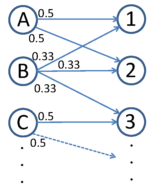
Figure 7: Small example extract of a probabilistic ranking as produced by our framework.

V-B U-$k$Ranks

The U-$k$Ranks [22] approach reports the most likely object instance at each rank $i$, i.e. the instance that is most likely to be ranked $i$th over all possible worlds. This is essentially the same definition as proposed in $PRank$ in [17] in the context of distributions over spatial data. The approach proposed in [22] has exponential runtime. The runtime has been reduced to $O(n^{2}k)$ time in [26]. Using our framework, the problem of U-$k$Ranks can be solved in $O(n\cdot log(n)+nk)$ time using the same space complexity as follows:
Use the framework to create the probabilistic ranking in $O(n\cdot log(n)+nk)$ as explained in the previous section. Then, for each rank $i$, find the object instance $argmax_{j}(p\_rank_{q}(o_{j},i))$ that has the highest probability of appearing at rank $i$ in $O(nk)$. This is performed by (cf. Figure 7) finding for each rank $i$ the object instance which has the highest probability to be assigned to rank $i$. Obviously, a problem of this problem definition is that a single object instance $o_{j}$ may appear at more than one ranking position, or at no ranking position at all. For example in 7, object instance $A$ is ranked on both ranks $1$ and $2$, while object instance $B$ is ranked nowhere. The total runtime for U-$k$Ranks has thus been reduced from $O(n^{2})$ to $O(nlog(n)+kn)$, that is $O(n*log(n))$ if $k$ is assumed to be constant.

V-C PT-$k$

The probabilistic threshold top-k query (PT-$k$) [13] problem fixes the problem of the previous definition by aggregating the probabilities of an object instance $o_{j}$ appearing at rank $k$ or better. Given a user-specified probability threshold $p$, PT-$k$ returns all instances, that have a probability of at least $p$ of being at rank $k$ or better. Note that in this definition, the number of results is not limited to $k$ and depends on the threshold parameter $p$. The model of PT-$k$ consists of a set of instances and a set of generation rules that define mutually exclusiveness of instances. Each object instance occurs in one and only one generation rule. This model conceptionally corresponds to the x-relation model (with disjoint x-tupels). PT-$k$ computes all result instances in $O(nk)$ time while also assuming that the instances are already pre-sorted, thus having a total runtime of $O(nlog(n)+kn)$.
The framework can be used to solve the PT-$k$ problem in the following way:
We create the probabilistic ranking in $O(nk)$ as explained in the previous section. For each object instance $o_{j}$, we compute the probability that $o_{j}$ appears at position $k$ or better (in $O(nk)$). Formally, we return all instances $o_{j}\in\mathcal{D}$ for which:

$$\{o_{j}\in\mathcal{D}|\sum_{i=1}^{k}p\_rank_{q}(o_{j},i)>p\}$$

As seen in Figure 7, this probability can simply be computed by aggregating all probabilities of an object instance to be ranked at $k$ or better. For example, for $k=2$ and $p=0.5$, we get $A$ and $B$ as results. Note that for $p=0.1$, further object instances may be in the result, because there must be further object instances (from object instances that are left out here for simplicity) with a probability greater than zero to rank $1$ and rank $2$, since the probability of their respective edges does not sum up to $1.0$ yet.

Note that our framework is only able to match, not to beat the runtime of PT-$k$. However, using our approach, we can additionally return the ranking order, instead of just the top-$k$ set.

V-D Global top-$k$

Global top-k [28] is very similar to PT-$k$ and ranks the object instances by their top-$k$ probability, and then takes the top-$k$ of these. This approach has a runtime of $O(n^{2}k)$. The advantage here is that, unlike in PT-$k$, the number of results is fixed, and there is no user-specified threshold parameter. Here we can exploit the ranking order information that we acquired in the PT-$k$ using our framework to solve Global top-k in $O(n\cdot log(n)+kn)$ time:
We use the framework to create the probabilistic ranking in $O(n\cdot log(n)+kn)$ as explained in the previous section. For each object instance $o_{j}$, we compute the probability that $o_{j}$ appears at position $k$ or better (in $O(nk)$) like in PT-$k$. Then, we find the $k$ object instances with the highest probability in $O(k\cdot log(k))$.

VI Experimental Evaluation

We have performed extensive experiments to evaluate the performance of our proposed probabilistic ranking approach proposed in Section III w.r.t. the database size ($|\mathcal{D}|$) measured in the number of uncertain vector objects, ranking depth ($k$) and degree of uncertainty (UD) as defined below. In the following, the ranking framework is briefly denoted by PSR.

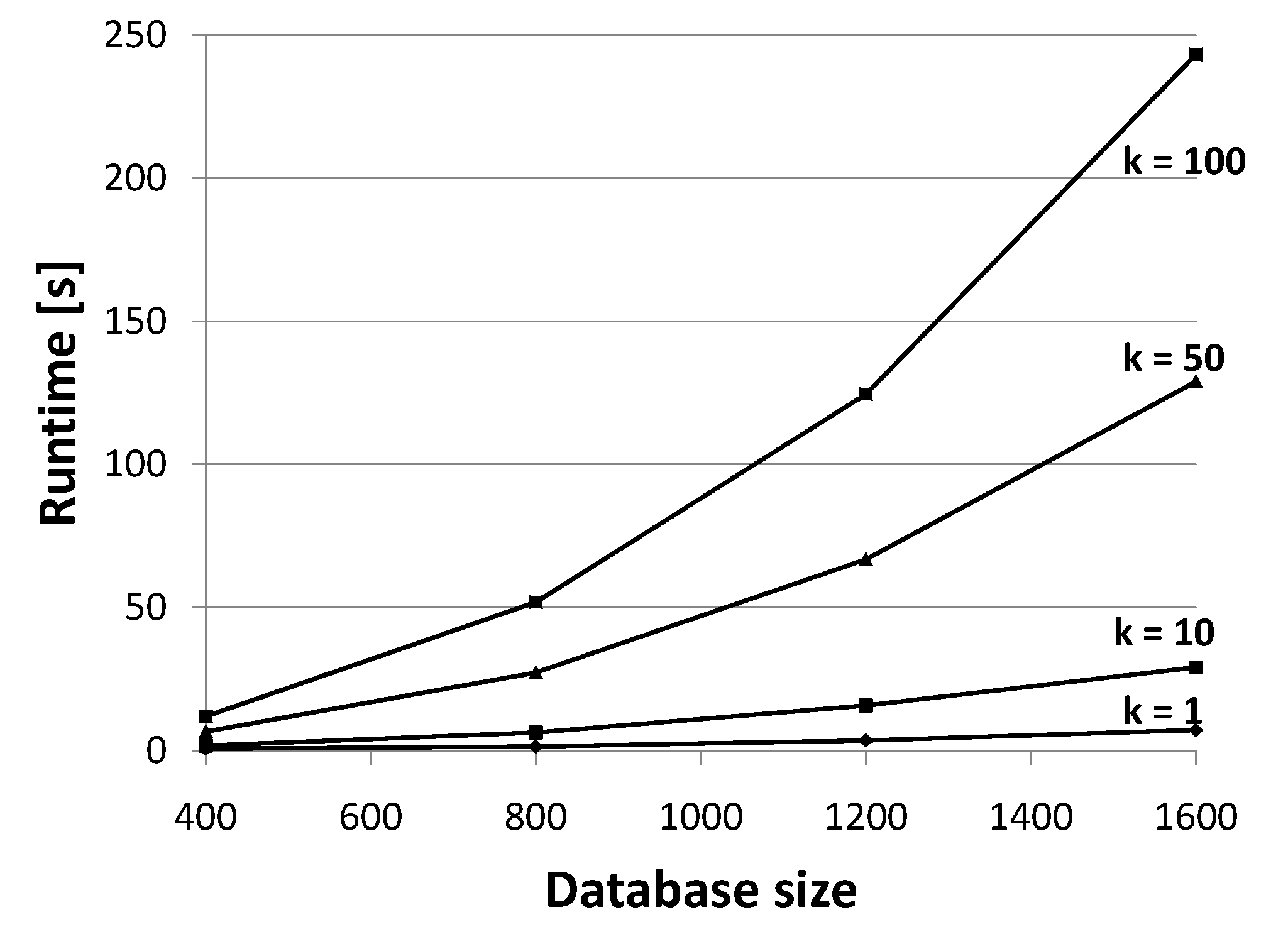
(a) YLKS

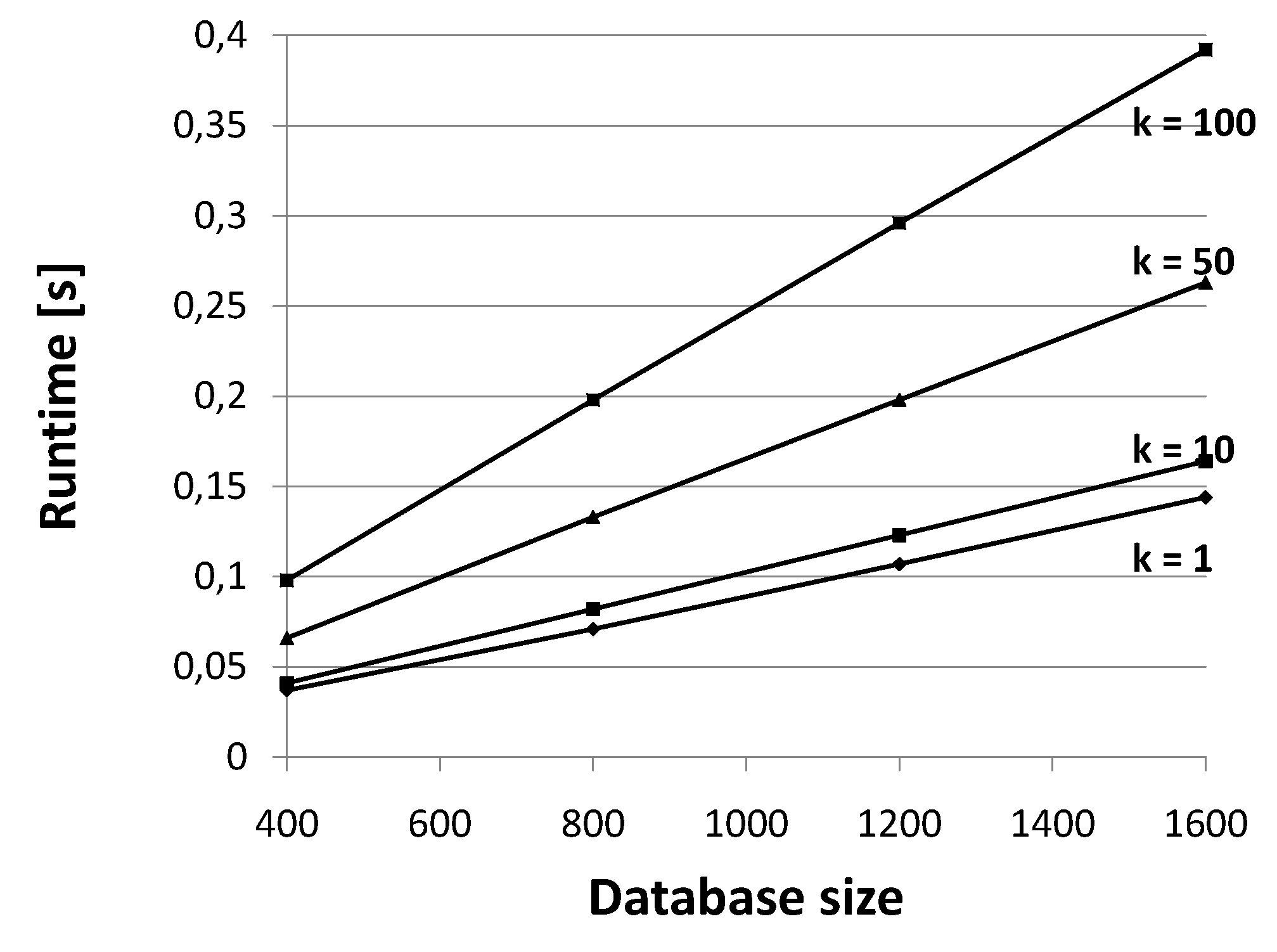
(b) PSR

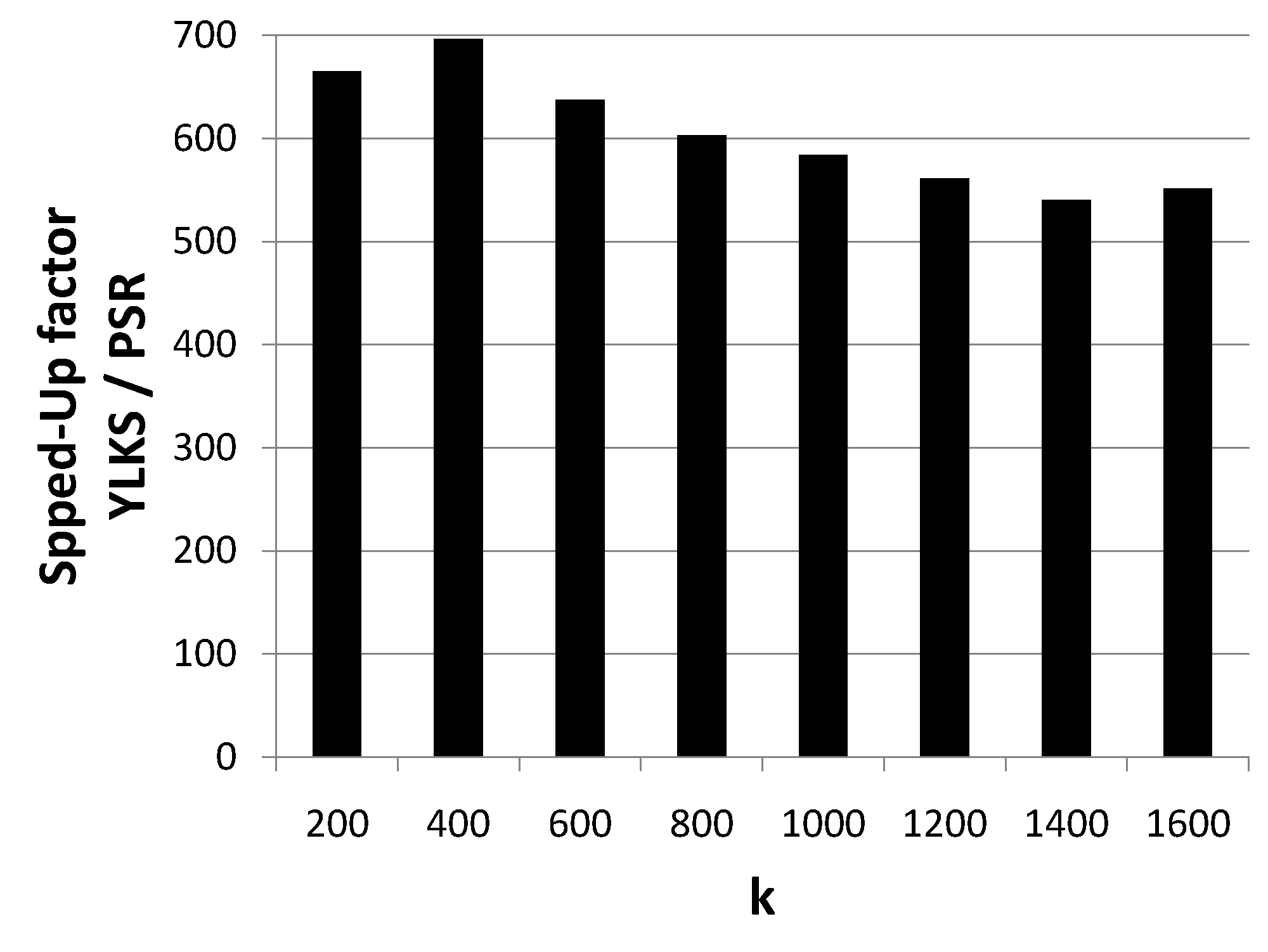
(c) Speed-up gain w.r.t. $k$ on SCI.

Figure 8: Scalability evaluated on SCI having different values for $k$.

VI-A Datasets and Experimental Setup

The probabilistic ranking was applied to a scientific real-world dataset SCI and several artificial datasets ART_X of varying size and degree of uncertainty. All datasets are based on the discrete uncertainty model, i.e. each object is represented by a collection of vector samples.

The SCI dataset is a set of 1600 objects where each object consists of 48 10-dimensional instances. Each instance corresponds to a set of environmental sensor measurements of one single day (one per 30 minutes) that consist of ten dimensions (attributes): Temperature, humidity, speed and direction of wind w.r.t. degree and sector, as well as concentrations of $CO$, $SO_{2}$, $NO$, $NO_{2}$ and $O_{3}$. These attributes are normalized within the interval [0,1] to give each attribute the same weight.

The ART_1 dataset consists of up to 1,000,000 objects for the scalability experiments. For the evaluation of the performance w.r.t. the ranking depth and the degree of uncertainty we applied a collection ART_2 of datasets each composing 10,000 objects. Each object is represented by a set of 20 3-dimensional instances. The ART_2 datasets differs in the degree of uncertainty ($UD$) the corresponding objects have. The degree of uncertainty ($UD$) reflects the following distribution of object instances: each uncertain vector object is assumed to be located within an 3-dimensional hyper-rectangle. The object instances are uniformly distributed within the corresponding rectangle. In the following, we will refer to the side length of the rectangles as degree of uncertainty ($UD$). The rectangles are uniformly distributed within a $10\times 10\times 10$ vector space.

The degree of uncertainty is interesting in our performance evaluation since it is expected to have a significant influence on the runtime. The reason is that a higher degree of uncertainty obviously leads to an higher overlap between the objects which influences the size of the active object list (AOL) (cf. Section IV) during the distance browsing. The higher the object overlap the more objects are expected to be in the AOL at a time. Since the size of the AOL influences the runtime of the rank probability computation, a higher degree of uncertainty is expected to lead to a higher runtime. This is experimentally evaluated in Section VI-D.

VI-B Scalability

In this section, we give an overview of our experiments regarding the scalability of PSR. We compare our results to the dynamic programming based rank probability computation used for the U-kRanks method as proposed by Yi et al. in [25]. This method, in the following denoted by YLKS, is the best approach currently known for solving the (instance-based) rank probability problem (cf. Table II). For a fair comparison, we used the PSR framework to compute the same (instance-based) rank probability problem as described in Section III. Let us note that the cost required to solve the object-based rank probability problem is similar to that required to solve the instance-based rank probability problem. This is because the former problem additionally only requires to build the sum over all instance-based rank probabilities which can be done on-the-fly without additional cost. Furthermore, we can neglect the cost required to build a final definite ranking (e.g. the rankings proposed in Section V) from the rank probabilities, because they can be also computed on-the-fly by simple aggregations of the corresponding (instance-based) rank probabilities.

For the sorting of the distances of the instances to the query point, we used a tuned quicksort adapted from [4]. This algorithm offers $O(n\cdot log(n))$ performance on many data sets that cause other quicksorts to degrade to quadratic performance.

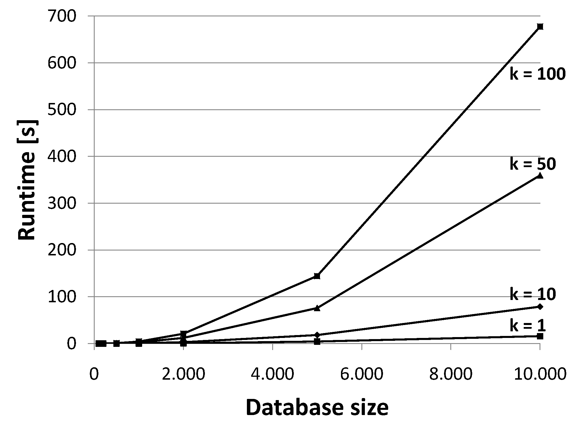
(a) YLKS

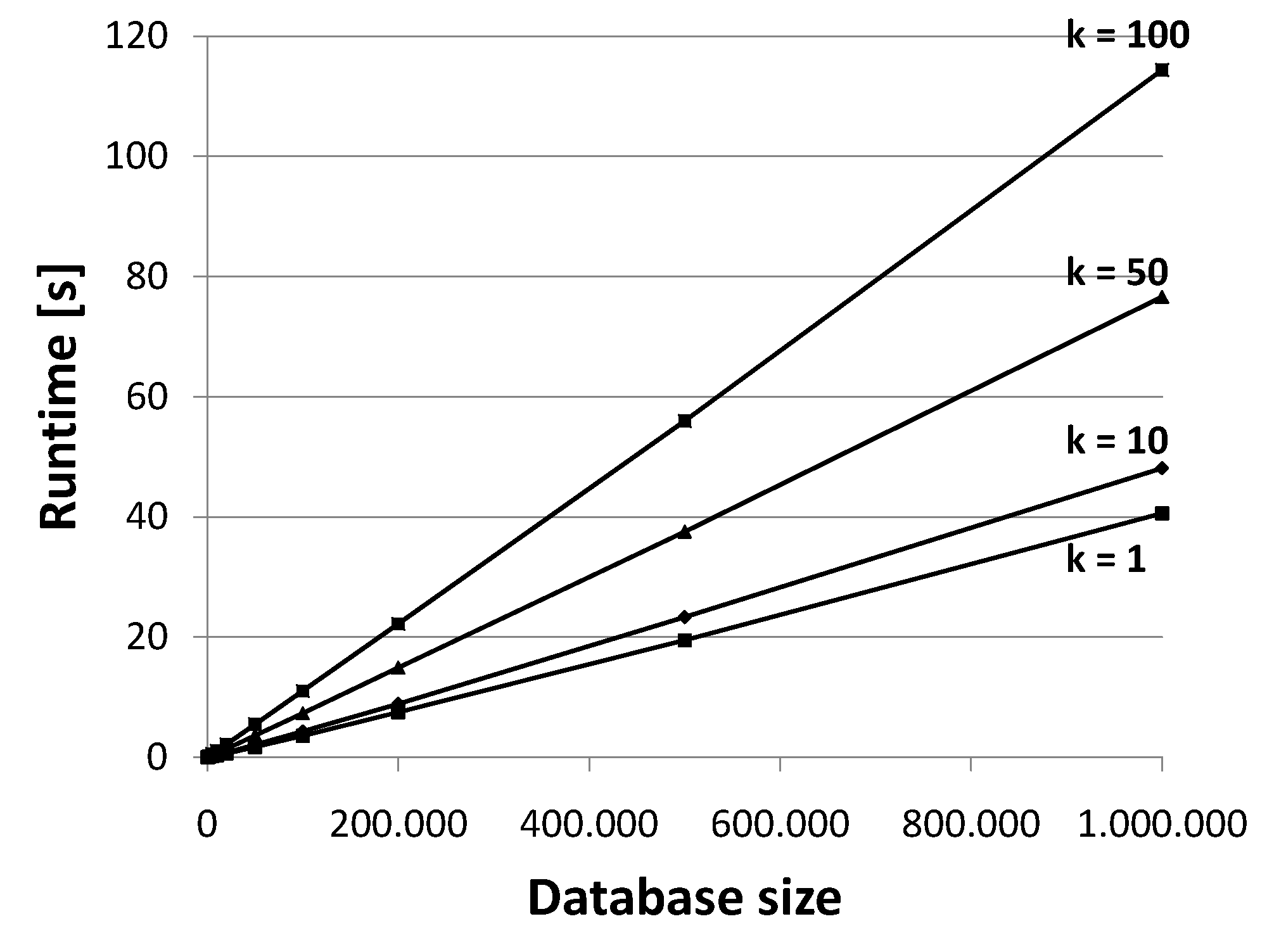
(b) PSR

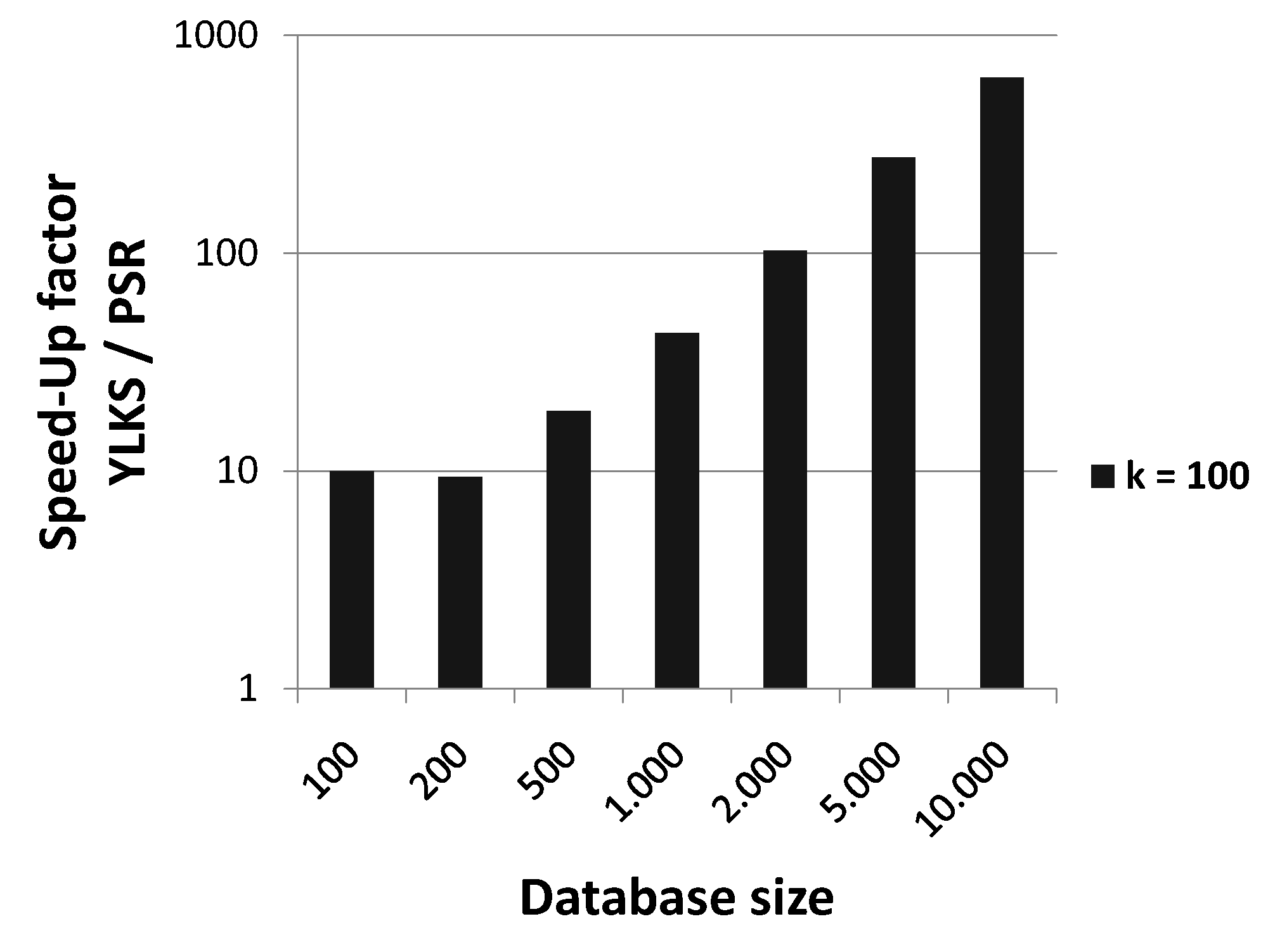
(c) Speed-up gain for an increasing $k$ grouped by an ascending number of objects in the database (ART_1 dataset).

Figure 9: Scalability evaluated on ART_1 w.r.t. $k$.

The results of our first scalability tests on the real-data set SCI are depicted in Figure 8. It can be observed in Figure 8(b) that the runtime of the probabilistic ranking using the PSR framework increases linearly in the database size, whereas YLKS has a runtime quadratic in the database size in the same parameter settings (cf. Figure 8(a)). We can also see that this effect persists for different settings of $k$. Note that the effect of the $O(n\cdot log(n))$ sorting of the distances of the instances is insignificant on this relatively small dataset. The direct speed-up of the rank probability computation using PSR in comparison to YLKS is depicted in Figure 8(c). It shows for different values of $k$, the speed-up factor, that is defined as the ratio $\frac{runtime(\textbf{YLKS})}{runtime(\textbf{PSR})}$ describing the performance gain of PSR vs. YLKS. It can be observed that, for a constant number of objects in the database ($|DB|=1600$), the ranking depth $k$ has no impact on the speed-up factor. This can be explained by the observation that both approaches scale linear in $k$.

Next, we evaluate the scalability of the database size based on the ART_1 dataset. The results of this experiment are depicted in Figure 9. Figure 9(b) shows that we are able to perform ranking queries in a reasonable time of less than 120 seconds, even for very large database containing 1,000,000 and more objects, each having 20 instances (thus having a total of 20,000,000 instances (tupels)). Note that the time required to sort the instances (less than 10 seconds for all 1,000,000 objects) is still insignificant compared to the total query cost. In Figure 9(a), it can be observed, that due to the quadratic scaling of the YLKS algorithm, it is inapplicable for relatively small databases of size $5000$ or more. The direct speed-up of the rank probability computation using PSR in comparison to YLKS for varying database size is depicted in Figure 9(c). Here, we can see that the speed-up of our approach in comparison to YLKS increases linear with the size of the database which is consistent with our runtime analysis in Section III.

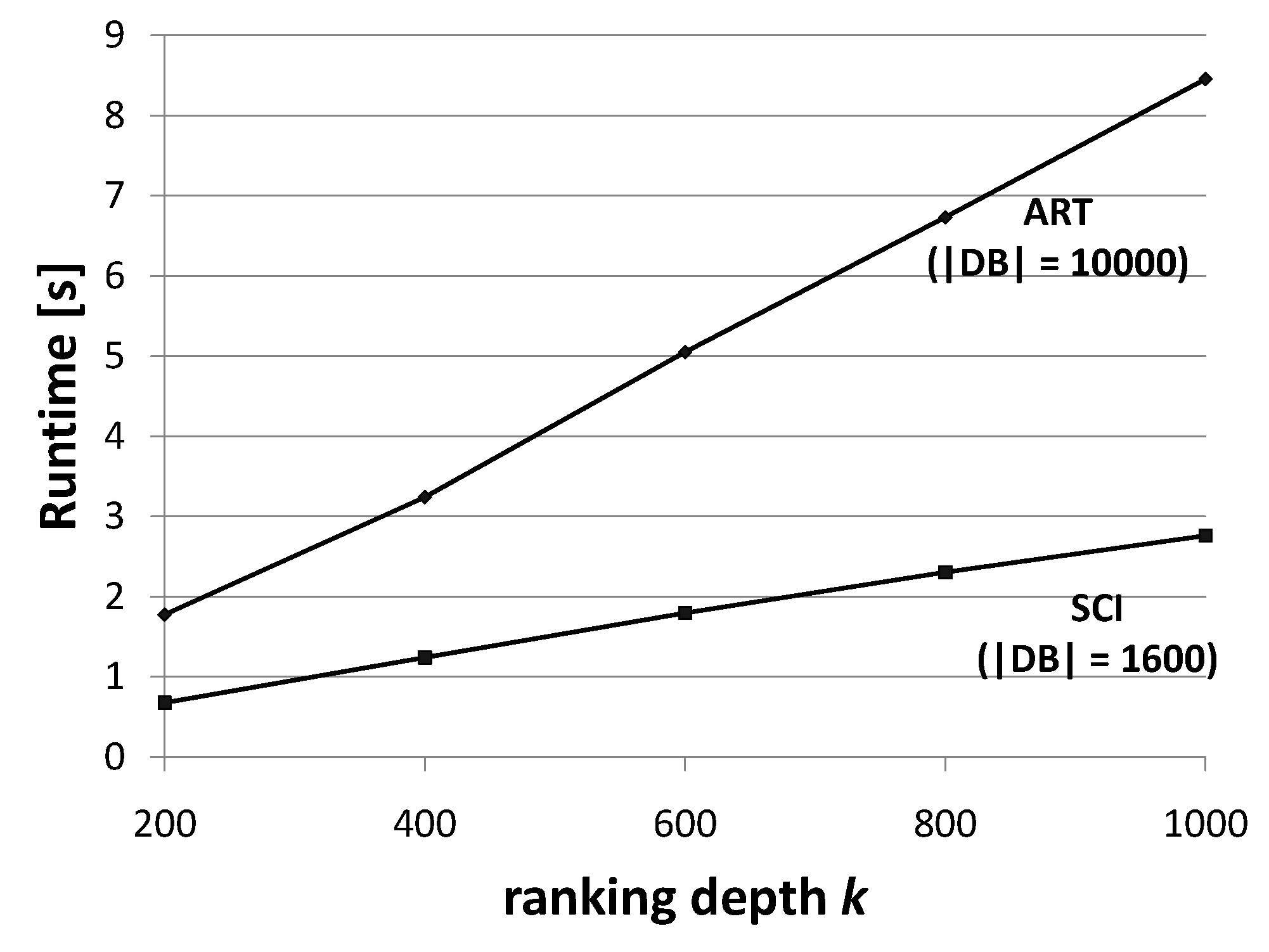
Figure 10: Runtime test using PSR on the datasets SCI and ART.

VI-C Ranking Depth $k$

The influence of the ranking depth $k$ on the runtime performance of our probabilistic ranking method PSR is studied in the next experiment. As depicted in Figure 10, where the experiments were performed using both the SCI and the ART dataset, the influence of an increasing $k$ yields a linear effect on the runtime of PSR, but does not depend on the type of the dataset. This effect can be explained by taking into consideration that each iteration of Case 2 or Case 3 requires a probability computation for each ranking position $0\leq i\leq k$.

VI-D Influence of the Degree of Uncertainty

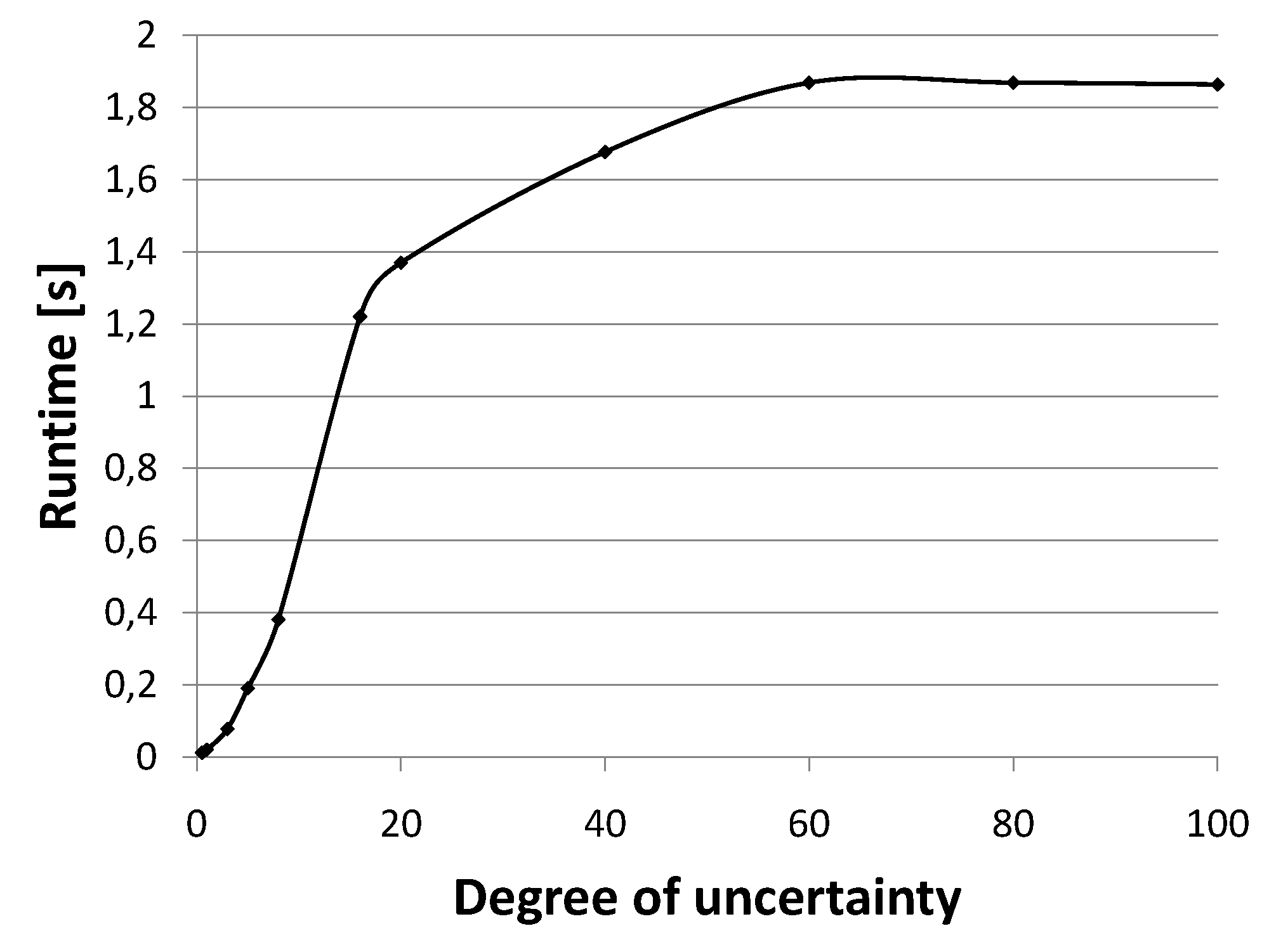
(a) Evaluation of PSR by an increasing uncertainty degree.

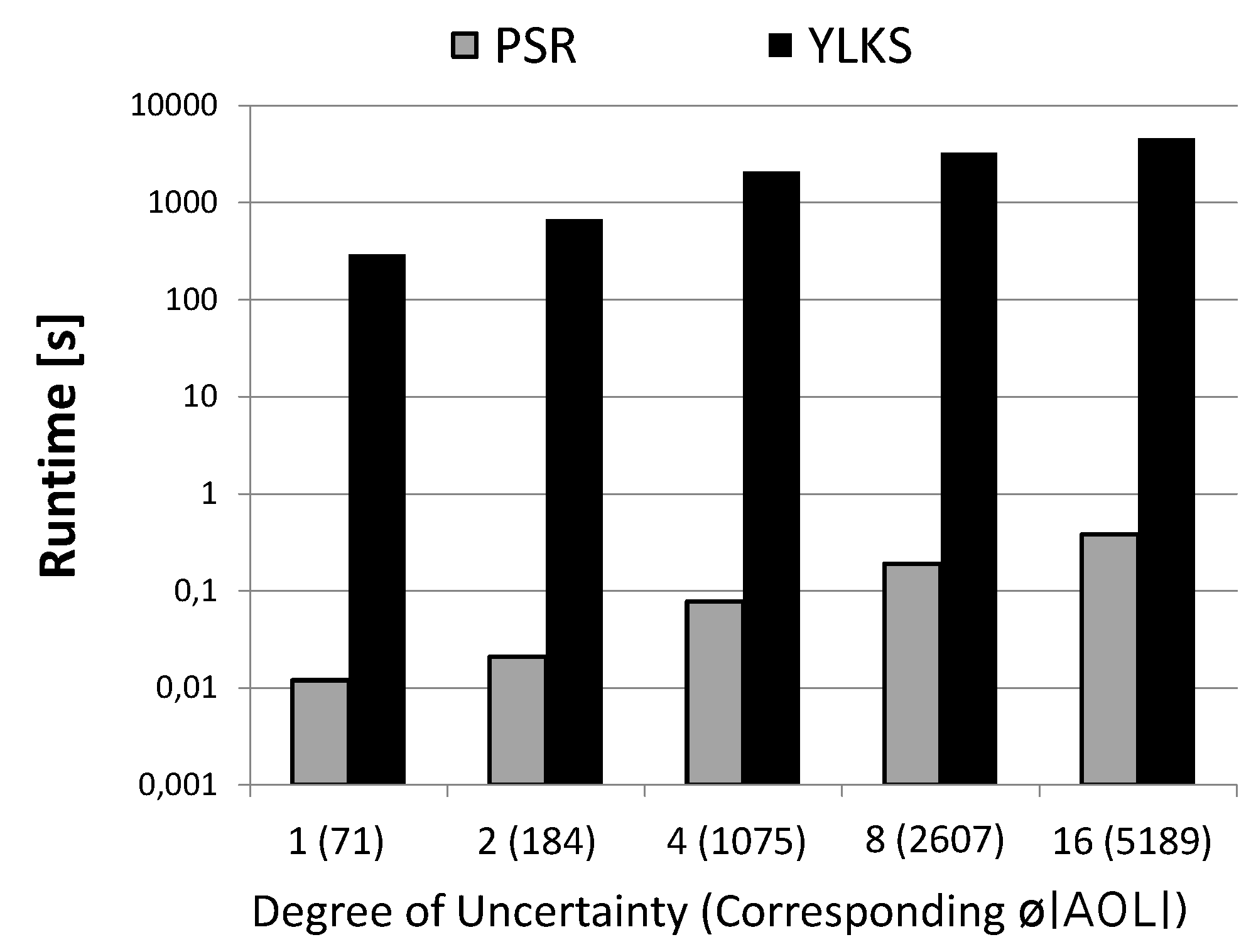
(b) YLKS vs. PSR in a logarithmic scale w.r.t. different $\varnothing(|AOL|)$ values.

Figure 11: Runtime test w.r.t. the degree of uncertainty.

In the next experiment, we varied the uncertainty degree of objects using the ART_2 dataset. In the following experiments, the ranking depth is set to a fixed value of $k=100$. As previously discussed, a varying degree of uncertainty leads to an increase of the overlap between the instances of the objects and thus, objects will remain in the $AOL$ for a longer time. The influence of the degree of uncertainty depends on the probabilistic ranking algorithm. This statement is underlined by the experiments shown in Figure 11. It can be seen in Figure 11(a) that PSR scales superlinear in the degree of uncertainty until a maximal value is reached. This maximal value is reached, when the degree of uncertainty approximates a uniform distribution on the whole vector space for all objects. With an increasing object uncertainty, the average number of active objects contained in the AOL grows, because the increased overlap of the object instances causes objects to stay in the AOL for a longer duration. A comparison of the runtime of YLKS and PSR w.r.t. the average AOL size is depicted in Figure 11(b).

VI-E Summary

The experiments presented in this section show that the theoretical analysis of our approach given in Section V can be confirmed empirically on both artificial and real-world data. The performance studies showed that our framework computing the rank probabilities indeed reduces the quadratic runtime complexity of state-of-the-art approaches to linear. Note that the cost required to pre-sort the object instances are neglected in our settings. It could be shown that our approach scales very well even for large databases. The speed-up gain of our approach w.r.t. the rank depth $k$ has shown to be constant, which proofs that both approaches scale linear in $k$. Furthermore, we could observe that our approach is applicable for databases with a high degree of uncertainty (i.e. the degree of variance of the instance distribution).

VII Conclusions

In this paper, we proposed a framework for efficient computation of probabilistic similarity ranking queries in uncertain vector databases. We introduced a novel concept that achieves a log-linear runtime complexity in contrast to the best-known existing approach that solve the same problem with quadratic runtime complexity. Our concepts are theoretically and empirically proved to be superior to all existing approaches. In an experimental evaluation, we showed that our approach scales very well and, thus, is applicable even for large databases. As future work, we plan to extend the concepts proposed in this paper to further uncertainty models.

References

- [1] P. Agrawal, O. Benjelloun, A. Das Sarma, C. Hayworth, S. Nabar, T. Sugihara, and J. Widom. ”Trio: A system for data, uncertainty, and lineage”. In Proc. Int. Conf. on Very Large Databases (VLDB’06), 2006.
- [2] L. Antova, T. Jansen, C. Koch, and D. Olteanu. ”Fast and Simple Relational Processing of Uncertain Data”. In Proc. 24th Int. Conf. on Data Engineering (ICDE’08), Canc n, M xico, 2008.
- [3] O. Benjelloun, A. D. Sarma, A. Halevy, and J. Widom. ”ULDBs: Databases with Uncertainty and Lineage”. In Proc. Int. Conf. on Very Large Databases (VLDB’06), pages 1249–1264, 2006.
- [4] J. L. Bentley and M. Douglas McIlroy. ”Engineering a Sort Function”.
- [5] T. Bernecker, H.-P. Kriegel, and M. Renz. Proud: Probabilistic ranking in uncertain databases. In In Proc. 20th Int. Conf. on Scientific and Statistical Database Management, Hong Kong, China, July 9-11, 2008.
- [6] C. B hm, A. Pryakhin, and M. Schubert. Probabilistic ranking queries on gaussians. pages 169–178, 2006.
- [7] R. Cheng, D. Kalashnikov, and S. Prabhakar. ”Evaluating Probabilistic Queries over Imprecise Data”. In Proc. ACM SIGMOD Int. Conf. on Management of Data (SIGMOD’03), San Diego, CA), pages 551–562, 2003.
- [8] R. Cheng, S. Singh, and S. Prabhakar. ”U-DBMS: a database system for managing constantly-evolving data”. In Proc. 31th Int. Conf. on Very Large Data Bases (VLDB’05), Trondheim, Norway, 2005.
- [9] R. Cheng, Y. Xia, S. Prabhakar, R. Shah, and J. Vitter. ”Efficient Indexing Methods for Probabilistic Threshold Queries over Uncertain Data”. In Proc. 30th Int. Conf. on Very Large Databases (VLDB’04), Toronto, Canada, pages 876–887, 2004.
- [10] G. Cormode, F. Li, and K. Yi. Semantics of ranking queries for probabilistic data and expected results. In Proceedings of the 25th International Conference on Data Engineering, ICDE 2009, March 29-April 2, 2009, Shanghai, China, pages 305–316, 2009.
- [11] N. Dalvi and D. Suciu. ”Efficient query evaluation on probabilistic databases”. The VLDB Journal, 16(4):523–544, 2007.
- [12] G. R. Hjaltason and H. Samet. Ranking in spatial databases. In In M. J. Egenhofer and J. R. Herring, editors, Advances in Spatial Databases - Fourth International Symposium, Portland, ME. (Also Springer-Verlag Lecture Notes in Computer Science 951.), pages 83–95, 1995.
- [13] M. Hua, J. Pei, W. Zhang, and X. Lin. Ranking queries on uncertain data: a probabilistic threshold approach. In Proceedings of the ACM SIGMOD International Conference on Management of Data, SIGMOD 2008, Vancouver, BC, Canada, June 10-12, 2008, pages 673–686, 2008.
- [14] H.-P. Kriegel, P. Kunath, M. Pfeifle, and M. Renz. ”Probabilistic Similarity Join on Uncertain Data”. In Proc. 11th Int. Conf. on Database Systems for Advanced Applications, Singapore, pp. 295-309, 2006.
- [15] H.-P. Kriegel, P. Kunath, and M. Renz. ”Probabilistic Nearest-Neighbor Query on Uncertain Objects”. In Proc. 12th Int. Conf. on Database Systems for Advanced Applications, Bangkok, Thailand, 2007.
- [16] H.-P. Kriegel, B. Seeger, R. Schneider, and N. Beckmann. The r*-tree: An efficient access method for geographic information system. In Proc. Int. Conf. on Geographic Information Systems, Ottawa, Canada, 1990.
- [17] X. Lian and L. Chen. Probabilistic ranked queries in uncertain databases. In EDBT 2008, 11th International Conference on Extending Database Technology, Nantes, France, March 25-29, 2008, Proceedings, pages 511–522, 2008.
- [18] V. Ljosa and A. Singh. Top-k spatial joins of probabilistic objects. In Proceedings of the 24th International Conference on Data Engineering, ICDE 2008, April 7-12, 2008, Cancún, México, pages 566–575, 2008.
- [19] C. Re, N. Dalvi, and D. Suciu. ”Efficient top-k query evaluation on probalistic databases”. In Proc. 23rd Int. Conf. on Data Engineering (ICDE’07), Istanbul, Turkey, 2007.
- [20] P. Sen and A. Deshpande. ”Representing and querying correlated tuples in probabilistic databases”. In Proc. 23rd Int. Conf. on Data Engineering (ICDE’07), Istanbul, Turkey, 2007.
- [21] M. Soliman and I. Ilyas. Ranking with uncertain scores. In Proceedings of the 25th International Conference on Data Engineering, ICDE 2009, March 29-April 2, 2009, Shanghai, China, pages 317–328, 2009.
- [22] M. Soliman, I. Ilyas, and K. Chen-Chuan Chang. Top-k query processing in uncertain databases. In Proceedings of the 23rd International Conference on Data Engineering, ICDE 2007, April 15-20, 2007, The Marmara Hotel, Istanbul, Turkey, pages 896–905, 2007.
- [23] Y. Tao, R. Cheng, X. Xiao, W. Ngai, B. Kao, and S. Prabhakar. ”Indexing Multi-Dimensional Uncertain Data with Arbitrary Probability Density Functions”. In Proc. 31th Int. Conf. on Very Large Data Bases (VLDB’05), Trondheim, Norway, pages 922–933, 2005.
- [24] O. Wolfson, P. Sistla, S. Chamberlain, and Y. Yesha. Updating and querying databases that track mobile units. Distributed and Parallel Databases, 7(3), 1999.
- [25] K. Yi, F. Li, G. Kollios, and D. Srivastava. Efficient processing of top-k queries in uncertain databases. In Proceedings of the 24th International Conference on Data Engineering, ICDE 2008, April 7-12, 2008, Cancún, México, pages 1406–1408, 2008.
- [26] K. Yi, F. Li, G. Kollios, and D. Srivastava. Efficient processing of top-k queries in uncertain databases with x-relations. IEEE Trans. Knowl. Data Eng., 20(12):1669–1682, 2008.
- [27] M. L. Yiu, N. Mamoulis, X. Dai, Y. Tao, and M. Vaitis. Efficient evaluation of probabilistic advanced spatial queries on existentially uncertain data. IEEE Trans. Knowl. Data Eng., 21(1):108–122, 2009.
- [28] X. Zhang and J. Chomicki. On the semantics and evaluation of top-k queries in probabilistic databases. In Proceedings of the 24th International Conference on Data Engineering Workshops, ICDE 2008, April 7-12, 2008, Cancún, México, pages 556–563, 2008.