The role of static stress diffusion in the spatio-temporal organization of aftershocks

Abstract

We investigate the spatial distribution of aftershocks and we find that aftershock linear density exhibits a maximum, that depends on the mainshock magnitude, followed by a power law decay. The exponent controlling the asymptotic decay and the fractal dimensionality of epicenters clearly indicate triggering by static stress. The non monotonic behavior of the linear density and its dependence on the mainshock magnitude can be interpreted in terms of diffusion of static stress. This is supported by the power law growth with exponent $H\simeq 0.5$ of the average main-aftershock distance. Implementing static stress diffusion within a stochastic model for aftershock occurrence we are able to reproduce aftershock linear density spatial decay, its dependence on the mainshock magnitude and its evolution in time.

Large earthquakes give rise to a sudden increase of the seismic rate in the surrounding area. Aftershocks are often observed where mainshocks have increased the static Coulomb stress rea ; kin ; har ; wys and their rate decays in time in agreement with state-rate friction laws die ; ste . Aftershocks also occur in regions of reduced static stress par as well as at distances up to thousand kms from the mainshock hil ; sta ; bro ; gom ; ebe ; gom2 . Dynamic stress related to the passage of shock waves, is the most plausible explanation for this remote triggering. Many studies, also supported by experiments on laboratory fault gouge systems joh , have recently proposed dynamic stress as the main mechanism responsible for aftershock triggering joh ; kil ; kil2 ; fel . The distribution $\rho(\Delta r)$, where $\Delta r$ is the epicentral distance between each aftershock and its related mainshock, represents a useful tool to discriminate between triggering by static or dynamic stress fel . In both cases, $\rho(\Delta r)$ is expected to decay asymptotically as $\Delta r^{-\mu}$, where $\mu$ is related to the fractal dimensionality $D$ of epicenters via the relationship $\mu+D-1=\alpha$ with $\alpha=1$ or $\alpha=2$ for dynamic or static stress triggering, respectively. Felzer & Brodsky (FB) fel studied $\rho(\Delta r)$ for small and intermediate mainshock magnitudes, obtaining a pure power law decay with an exponent $\mu\simeq 1.4$. This result, together with the estimate $D\simeq 1$, was interpreted in favor of dynamic stress triggering aftershocks. In this paper we will show that the distribution $\rho(\Delta r)$ exhibits a non-monotonic behavior, with a power law tail and a maximum depending on the mainshock magnitude that can be attributed to a stress diffusion mechanism.

In our analysis we use the Shearer et al. relocated Southern California Catalogue in the years 1981-2005 she with an average uncertainty on the epicentral localization of $0.03$ km. We consider all events with magnitude $m\geq 2$. Mainshocks are identified with the same criterion used by FB, i.e mainshocks are events separated in time and space from larger earthquakes fel . Aftershocks are all subsequent events occurring within a circular region of radius $100$ km centered at the mainshock epicenter. In Fig.1 we plot $\rho(\Delta r)$ for all aftershocks related to a mainshock with magnitude $m\in[M,M+1[$ for $M=2,3,4$ and for a typical time window of 30 min post-mainshock, as considered by FB. We find that $\rho(\Delta r)$ exhibits a maximum at a value of $\Delta r$ increasing with $M$, followed by a pure power law decay $\Delta r^{-1.9}$ only when $M=4$. For $M=2,3$, conversely, a plateau is observed at large distances, $\Delta r>10km$ ($M=2$) and $\Delta r>30km$ ($M=3$), which is related to uncorrelated background events. Indeed, $\rho(\Delta r)$ can be written as the sum $\rho(\Delta r)=\rho_{AS}(\Delta r)+\rho_{B}(\Delta r)$, where $\rho_{AS}(\Delta r)$ is the aftershock density distribution and $\rho_{B}(\Delta r)\propto\Delta r^{D-1}$ is the contribution of background events. Since the aftershock number decreases in time whereas background seismicity has a constant rate, $\rho(\Delta r)\simeq\rho_{B}(\Delta r)$ in temporal windows sufficiently distant from the mainshock. More precisely, we obtain $\rho_{B}(\Delta r)$ in temporal widows distant more than $t_{d}=70$ days from the mainshock. Results, plotted as open symbols in Fig.1, do not depend on $t_{d}$ for larger $t_{d}$. For each $M$, a flat behaviour is obtained for $\Delta r>1$ km, implying $D\simeq 1$, in agreement with FB. A more precise measurement gives $D=1.03\pm 0.05$. The value of $\rho_{B}(\Delta r)$ depends on $M$, since it is proportional to the number of mainshocks in each class $M$. This implies that $\rho_{B}(\Delta r)$ becomes less relevant for larger $M$ and, in particular, does not affect the exponent $\mu=1.88\pm 0.05$ obtained for $M=4$ from Fig.1. For $M=2,3$, conversely, the tail of the distribution must be appropriately fitted with $\rho(\Delta r)=\rho_{B}(\Delta r)+A\Delta r^{-\mu}$. For $\Delta r>1$ km, the correlation coefficient provides results consistent with $\mu=2$ and excludes $\mu=1.4$. Hence, the exponent value $\mu\simeq 1.4$ obtained as best fit in the range $[0.2:50]$ km (orange line in Fig. 1b) does not represent the asymptotic decay of $\rho(\Delta r)$. Similar behavior is obtained for hypocentral distances, with small differences only at lengths comparable with location errors.

In order to extend the analysis to larger temporal windows post-mainshock we use the criterion proposed in ref. bai to separate aftershocks from background events. Given two events with magnitude $m_{1}$ and $m_{2}$ with occurrence times $t_{1}<t_{2}$ and locations $\vec{r}_{1},\vec{r}_{2}$, the expected number of events inside a circle of radius $\Delta r=|\vec{r}_{1}-\vec{r}_{2}|$ centered in $\vec{r}_{1}$, over a time window $T=t_{2}-t_{1}$ is proportional to $n_{exp}(1,2)=C10^{-b(m_{1}-2)}T\Delta r^{D}$. Here $D=1.03$, $b$ is the slope of the Gutenberg-Richter magnitude-frequency distribution and $C=2.06\ \ 10^{-11}sec^{-1}km^{-D}$ is the average rate of $m\geq 2$ earthquakes in the catalog. For a given mainshock $(\vec{r}_{1},t_{1})$ each subsequent earthquake ($\vec{r}_{2},t_{2}$) with $n_{exp}(1,2)<n_{th}\ll 1$, where $n_{th}$ is a given threshold, is highly unexpected and therefore it is considered an aftershock. Aftershock number should decay in time according to the Omori law, which fixes the value of the threshold $n_{th}$, in particular we find $n_{th}=10^{-3}$. Different values of $D\in[1.1,1.6]$ provide similar results. This criterion allows to discriminate between aftershocks directly triggered by the mainshock (first generation) from higher order generations, excluding eventual effects due to aftershock cascading hel ; huc ; mck ; mar . An event $2$ is a first generation aftershock of the event $1$, if in the time interval $]t_{1},t_{2}[$ no event $j$ with $n(j,2)\leq n(1,2)$ is present. All the following results are obtained considering only first generation aftershocks. No important difference is observed if higher order generation aftershocks are included in the analysis. The study of $\rho_{AS}(\Delta r)$ with this aftershock selection criterion (Fig.2) provides results in agreement with the previous analysis, i.e. a power law decay with an exponent $\mu\simeq 2$ for all values of $M$. Furthermore, curves for different $M$ collapse on the same master curve (inset a of Fig.2) following the scaling

$$\rho(\Delta r)=10^{-\beta M}F\left(\frac{\Delta r}{10^{\beta M}}\right)$$ (1)

with $\beta=0.42\pm 0.02$. This result was obtained in ref. bai using a different mainshock selection criterion. The function $F(x)$ is non monotonic and exhibits power law behaviour $F(x)\sim x^{-\mu}$ with $\mu=1.94\pm 0.04$ at large $x$. The collapse of curves with small $M$ on curves with larger $M$, weakly affected by the background seismicity, validates the aftershock selection criterion. Fig.2 confirms $\mu\simeq 2$ supporting the static stress triggering scenario.

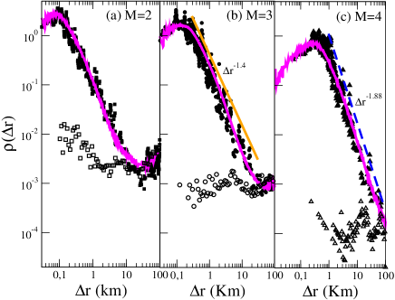
Figure 1: (Color online) The distribution of distances from the mainshock (filled symbols) versus $\Delta r$ for mainshock magnitude $m\in[M,M+1[$. Aftershocks are events occurring within $T=30min$ from the mainshock ($678,864,494$ aftershocks for $M=2,3,4$ respectively). Open symbols represent $\rho_{B}(\Delta r)$. For $M=4$, the power law fit in the range $[1:100]$ km gives $\mu=1.88\pm 0.05$ (dashed blue line in panel c). Magenta curves are obtained by adding the experimental $\rho_{B}(\Delta r)$ to the numerical $\rho(\Delta r)$. The orange line in panel (b) is the power law $x^{-1.4}$ obtained by FB in the intermediate range $[0.2:16]$km.

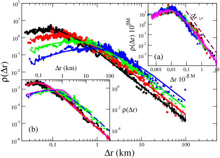
Figure 2: (Color online) The distribution of distances from the mainshock for $M=2$ (circles), $M=3$ (squares), $M=4$ (diamonds) and $M=5$ (triangles). Aftershocks are events occurring within $T=5h$ from the mainshock. The aftershock (mainshock) number is $1065$ ($12746$) for $M=2$, $1800$ ($3410$) for $M=3$, $1425$ ($349$) for $M=4$ and $1454$ ($52$) for $M=5$. Continuous lines are the result of numerical simulations. In the inset (a), collapse of the curve is obtained rescaling $\Delta r$ by $10^{\beta M}$ according to Eq.(1), with $\beta=0.42$. The continuous magenta line is the theoretical master curve $F(x)$ and the brown dashed line shows the asymptotic decay $F(x)\sim x^{-2}$. In the inset (b), comparison of experimental $\rho(\Delta r)$ for $M=2,4$ (symbols) with the theoretical predictions $\rho_{th}(\Delta r)$ (continuous magenta lines). Dashed lines (red $M=2$, blue $M=4$) are the results of the stochastic model simulations.

The non-monotonic behaviour of $\rho(\Delta r)$ is commonly attributed to the violation of the point-source hypothesis fel . This implies that seismic sources have a finite extension whose linear size scales with the earthquake magnitude $L_{S}(m)=0.01\ \ 10^{0.5m}$ km Kagan . One then computes $\rho_{th}(\Delta r)$ assuming that aftershocks are distributed according to a power law from a point randomly chosen on the mainshock fault and defining $\Delta r$ as the distance from the center of the mainshock fault. $\rho_{th}(\Delta r)$ follows the experimental $\rho(\Delta r)$ in the whole spatial range for $M=2$ (inset (b) in Fig.2). For larger $M$, conversely, theoretical curves significantly deviates from the experimental ones. Indeed, curves for different $M$ collapse on the same pure power law decay at distances $\Delta r>L_{S}(m)$, where the point source hypothesis holds. This implies that, even if theoretical curves exhibit a non-monotonic behavior, they do not verify the scaling collapse Eq(1).

The scaling behavior of $\rho(\Delta r)$ can be attributed to a diffusion process. To this extent, we implement static stress diffusion in a stochastic model for seismic occurrence based on a dynamical scaling assumption lip ; lip2 ; lip3 . Within this framework, for a given mainshock of magnitude $m_{0}$ and an aftershock of magnitude $m$, the magnitude difference $\Delta m=m_{0}-m$, $\Delta r$ and $\Delta t$ are not independent variables. More precisely, if time is rescaled by a a generic scaling factor $\lambda$, $\Delta t\to\lambda\Delta t$, the statistical properties are invariant provided that $\Delta r\to\lambda^{H}\Delta r$ and $\Delta m\to\Delta m+(1/b)\log\lambda$, where $H$ is a scaling exponent. The scaling relation among $\Delta t$, $\Delta r$ and $\Delta m$ implies that, for a given mainshock of magnitude $m_{0}$, the conditional probability to have a magnitude $m$ aftershock at distance $\Delta r$ after a time $\Delta t$, takes the scaling form $P(\Delta t,\Delta r,m,m_{0})=\Delta t^{-H}G_{t}\left(\frac{10^{b(m_{0}-m)}}{\Delta t}\right)G_{r}\left(\frac{\Delta r}{\Delta t^{H}}\right)$. Under the only assumption that $G_{t}(y)$ and $G_{r}(x)$ are normalizable functions, one recovers several features of seismic occurrence as the GR law, the generalized Omori law, the scaling behavior of the intertime distribution lip . The distribution $\rho(\Delta r)$ can be obtained by integrating $P(\Delta t,\Delta r,m,m_{0})P(m_{0})$ over $\Delta t$ and $m$. The scaling relation for $P(\Delta t,\Delta r,m,m_{0})$ and the GR law $P(m_{0})\sim 10^{-bm_{0}}$ then give Eq.(1), with $F(x)\propto\int_{0}^{\infty}du\int_{0}^{\infty}dvu^{-1}v^{-H}G_{t}(u/v)G_{r}(xv^{-H})$ and $\beta=bH$. Assuming the power law decay $G_{r}(x)\propto x^{-\mu}$, for $x$ larger than a cut-off $x_{0}$, $F(x)$ is a non-monotonic function with an asymptotic decay $F(x)\sim x^{-\mu}$ for $x\gg 1$. We therefore implement in the numerical simulations the parameters fitted from experimental data, $\mu=2$ and $H=0.47$, obtained from $\beta=0.42$ and the typical value $b=0.9$. In particular, following the procedure described in lip2 , we set $G_{t}(y)\propto\left(e^{1/(k_{t}y)}-1+\gamma_{1}\right)^{-1}$ with the parameters $k_{t}=12.7h$, $\gamma_{1}=0.1$, $b=0.9$, and $G_{r}(x)\propto(k_{r}x)^{-\mu}$ for $x>x_{0}$ with $\mu=2$, $H=0.48$, $k_{r}=5.1\ \ 10^{-6}km^{z}/sec$ and $x_{0}=3\ \ 10^{-3}km/sec^{z}$. We find that, for all values of $M$, numerical curves follow the experimental ones (Fig.2). The scaling (1) is fulfilled with the numerical $F(x)$ reproducing the experimental master curve (inset (a) of Fig.2). As a further check, we add $\rho_{B}(\Delta r)$, obtained in Fig.1, to the numerical distribution $\rho(\Delta r)$. Numerical results (Fig.1) very well agree with experimental data over the entire spatial range.

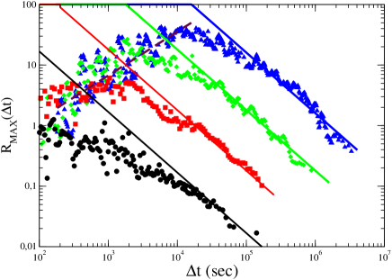
Figure 3: (Color online) The maximum distance $R_{MAX}(\Delta t)$ for $M=2,3,4,5$ (circles, squares, diamonds, triangles) from bottom to top. $R_{MAX}(\Delta t)$ grows until $\Delta t_{M}$ ($\Delta t_{M}=16000sec,2900sec,690sec,190sec$ for $M=5,4,3,2$). The dashed line is the power law fit $R_{MAX}(\Delta t)\sim\Delta t^{H}$ with $H=0.54\pm 0.05$ obtained for $M=5$ and $\Delta t<\Delta t_{M}$. Continuous lines are the theoretical prediction for $L_{MAX}(\Delta t)$.

The agreement between experimental and numerical results supports the validity of the scaling relation $\Delta r\sim\Delta t^{H}$ with $H\simeq 0.5$, which implies that the evolution in time of stress is consistent with a diffusion equation. More direct evidence of static stress diffusion can be obtained by the temporal evolution of the main-aftershock spatial distance. In particular we compute $R_{MAX}(\Delta t)$ ($R(\Delta t)$), i.e. the maximum (average) distance from a mainshock with $m\in[M,M+1[$, of aftershocks occurring in the time window $[\Delta t,\Delta t(1+\epsilon)]$. For all $M$, $R_{MAX}(\Delta t)$ exhibits (Fig.3) a non monotonic behaviour with a maximum at a $M$-dependent typical $\Delta t_{M}$. $\Delta t_{M}$ can be identified as the time when the percentage of events identified as aftershocks becomes smaller than the $90\%$ of the total number of recorded earthquakes. Therefore, for $\Delta t<\Delta t_{M}$, no significant bias related to the aftershock selection procedure is present. In this temporal regime, similar results are obtained including in the analysis all subsequent earthquakes occurring within a radius of $100$ kms from the mainshock. Fig.3 shows that, for all values of $M$, $R_{MAX}$ increases for times $\Delta t<\Delta t_{M}$. For $M=5$ where $\Delta t_{M}=16000sec$, a power law regime $R_{MAX}(\Delta t)\sim\Delta t^{H}$ clearly detected with $H=0.54\pm 0.05$. On the other hand, the decay for $\Delta t>\Delta t_{M}$ originates from a bias introduced by the method for aftershock selection. The condition $n_{exp}(1,2)<n_{th}$, indeed, implies that aftershocks are only events occurring within a given temporal-magnitude region and, in particular, all events occurring at distances larger than $L_{MAX}(\Delta t)\propto 10^{Mb/D}(\Delta t)^{-1/D}$ are not considered as aftershocks. The tails of $R_{MAX}(\Delta t)$ are consistent with a pure power law decay $\Delta t^{-1/D}$ in agreement with the analytical expression for $L_{MAX}(\Delta t)$ (Fig.3).

Further indication of diffusion can be obtained in the regime $\Delta t>\Delta t_{M}$ by considering the average distance $R(\Delta t)$ inside a region of radius $L_{sup}$. This can be evaluated as $R(\Delta t)=\int_{0}^{L_{sup}}d\Delta r\Delta r\rho(\Delta r)/\int_{0}^{L_{sup}}d\Delta r\rho(\Delta r)$, using the decay $\rho(\Delta r)\propto(\Delta r+K)^{-2}$ obtained from Fig.2

$$R(\Delta t)=K\left[\left(1+\frac{K}{L_{sup}}\right)\log\left(1+\frac{L_{sup}}{K}\right)-1\right].$$ (2)

According to the previous analysis $L_{sup}=100$ km when $\Delta t<\Delta t_{M}$ and $L_{sup}=L_{MAX}(\Delta t)$ when $\Delta t>\Delta t_{M}$. We introduce in the above equation $K=B\Delta t^{H}$ with $B=0.018km/sec^{H}$ and $H=0.47$, obtained from the numerical simulations. Fig.4 shows that for all $M$, without any further parameter tuning, the theoretical prediction (2) reproduces experimental results in the whole time range. In Fig.4 we also plot Eq.2 assuming a constant $K$, obtained as the best fit from Fig.2. In this case, the theoretical $R(\Delta t)$ (dashed lines in Fig.4) overestimates the experimental $R(\Delta t)$ at small $\Delta t$, whereas it somehow underestimates it at larger times. Previous analyses hel ; huc ; mck ; mar have obtained a smaller value of the diffusion exponent, $H\simeq 0.1$. The basic differences with our study is that in previous analyses aftershocks have not been classified according to the mainshock magnitude and distances significantly smaller than the mainshock fault length have been included in the analysis. Interestingly, McKernon and Main mck recover $H\simeq 0.5$ at very large distances, where the point source hypothesis is recovered.

Figure 4: (Color online) The average spatial distance $R(\Delta t)$ from the mainshock (black circles) of aftershocks occurring in the time window $[\Delta t,\Delta t(1+\epsilon)]$ with $\epsilon=0.02$ versus $\Delta t$. The initial growth $R(\Delta t)\sim\Delta t^{0.47}$ (magenta line) is consistent with the diffusion behaviour. The decay at larger times is related to the upper cut-off $L_{sup}$. Continuous red and dashed green curves are the theoretical prediction Eq.(2): Green curves correspond to $K=1.8\ \ 10^{0.42(M-5)}$ km fitted from Fig.2. Red curves correspond to $K=0.018\ \ \Delta t^{0.47}$ km, where $\Delta t$ is measured in seconds, obtained from the numerical model.

In conclusion, we have shown that static stress is the main mechanism responsible for aftershock occurrence. Indeed, by properly taking into account background seismicity, $\rho(\Delta r)$ exhibits the scaling behavior (1) with the power law decay expected within the static stress triggering scenario. Moreover, the very good agreement of the theoretical prediction (2) with the numerical results and experimental data indicates that the aftershock spatial organization evolves in time according to a diffusion equation. Migration of aftershocks mog is often observed and interpreted within different contexts, including state/rate friction die ; ste , viscoelastic relaxation process ryd ; fre ; jon and aftershock cascading hel ; huc ; mck ; mar . In the present study, the latter mechanism can be discarded, since only aftershocks directly triggered by the mainshock have been considered. The estimated value $B=0.018km/sec^{H}$ predicts, on average, a post seismic stress change over a region of about $10^{2}$ km in $7$ years. This is consistent with simulations of $3d$ viscoelastic post seismic relaxation after the 1992 Landers earthquake fre .

References

- (1) Reasenberg, P.A., Simpson, R.W., Science 255, 1687 (1992).
- (2) King, G.C.P., Stein, R.S., Lin, J., Bull. Seism. Soc. Am. 84, 935 (1994).
- (3) Hardebeck, J.L., Nazareth, J.J., Hauksson, E., J. Geophys. Res. -Solid Earth 103, 24427 (1998).
- (4) Wyss, M., Wiemer, S., Science 290, 1334 (2000).
- (5) Dieterich, JH. J. Geophys. Res 99, 2601 (1994).
- (6) Stein R.S., Nature 402, pp. 605-609 (1999).
- (7) Parsons, T., J. Geophys. Res. 107 2199,1, (2002).
- (8) Hill D.P. et al., Science 260, 1617, (1993).
- (9) Stark,M.A., Davis, S.D., Geophys. Res. Lett. 23, 945, (1996).
- (10) Brodsky, E.E., Karakostas, V., Kanamori, H., Geophys. Res. Lett. 27, 2741, (2000).
- (11) Gomberg,J., Reasenberg, P.A., Bodin, P., Harris, R.A., Nature 411, 462, (2001).
- (12) Eberhart-Phillips, D., et al., Science 300, 1113, (2003).
- (13) Gomberg, J., Bodin, P., Larson, K., Dragert, H., Nature 427, 621, (2004).
- (14) Johnson, P, Jia, X., Nature 437, 871, (2005).
- (15) Kilb, D., Gomberg, J., Bodin, P., Nature 408, 570, (2000).
- (16) Kilb, D., Gomberg, J., Bodin, P., J. Geophys. Res. 107 doi:10.1029/2001JB0002002, (2002).
- (17) Felzer, K.R., Brodsky, E.E., Nature 441, 735, (2006).
- (18) Shearer, P., Hauksson, E., Lin, G., Bull. Seismol. Soc. Am. 95, 904, (2005).
- (19) Baiesi, M., Paczuski, M., Phys. Rev. E 69, 0661061 (2004).
- (20) Helmstetter, A., Sornette, D., Phys. Rev. E , 66 , 061104, (2002).
- (21) Huc, M., Main, I.G., J.Geophys.Res., 108, 2324, (2003).
- (22) McKernon, C., Main, I.G., J. Geophys. Res., 110, B05S05, (2005).
- (23) Marsan, D. & Lengliné, O., Science, 319, 1076, (2008).
- (24) Kagan Y.Y., BSSA 92, 641 (2002).
- (25) Lippiello, E., Godano, C., de Arcangelis, L., Phys. Rev. Lett. 98, 098501 (2007).
- (26) Lippiello, E., de Arcangelis,L., Godano, C., Phys. Rev. Lett. 100, 038501 (2008).
- (27) Lippiello, E., Bottiglieri, M., Godano,C., de Arcangelis, L., Geophys. Res. Lett. 34, L23301 (2007).
- (28) Mogi, K., 1968,Bull.Earth. Res.Inst.Univ.Tokyo 46, 57, (1968).
- (29) Rydelek, P.A., Sacks, I.S., Nature, 336, 234, (1988).
- (30) Freed, A.M., Lin, J., Nature 441, 180, (2001).
- (31) Jónsson, S., Nature Geoscience 1, 136 (2008).