General Spectrum Sensing in Cognitive Radio Networks

Abstract

It is well known that the successful operation of cognitive radio (CR) between CR transmitter and CR receiver (CR link) relies on reliable spectrum sensing. To network CRs requires more information from spectrum sensing beyond traditional techniques, executing at CR transmitter and further information regarding the spectrum availability at CR receiver. Redefining the spectrum sensing along with statistical inference suitable for cognitive radio networks (CRN), we mathematically derive conditions to allow CR transmitter forwarding packets to CR receiver under guaranteed outage probability, and prove that the correlation of localized spectrum availability between a cooperative node and CR receiver determines effectiveness of the cooperative scheme. Applying our novel mathematical model to potential hidden terminals in CRN, we illustrate that the allowable transmission region of a CR, defined as neighborhood, is no longer circular shape even in a pure path loss channel model. This results in asymmetric CR links to make bidirectional links generally inappropriate in CRN, though this challenge can be alleviated with the aid of cooperative sensing. Therefore, spectrum sensing capability determines CRN topology. For multiple cooperative nodes, to fully utilize spectrum availability, the selection methodology of cooperative nodes is developed due to limited overhead of information exchange. Defining reliability as information of spectrum availability at CR receiver provided by a cooperative node and by applying neighborhood area, we can compare sensing capability of cooperative nodes from both link and network perspectives. In addition, due to dynamic network topology lack of centralized coordination in CRN, CRs can only acquire local and partial information in limited sensing duration, robust spectrum sensing is therefore proposed to ensure successful CRN operation. Limits of cooperative schemes and their impacts on network operation are also derived.

I Introduction

Cognitive radios (CR) [1][3], having capable of sensing spectrum availability, is considered as a promising technique to alleviate spectrum scarcity due to current static spectrum allotment policy [2]. Traditional CR link availability is solely determined by the spectrum sensing conducted at the transmitter (i.e. CR-Tx). If the CR-Tx with packets to relay senses the selected channel to be available, it precedes this opportunistic transmission. To facilitate the spectrum sensing, at time instant $t_{n}$, we usually use a hypothesis testing as follows.

$$H_{1}:Y =I+N$$ (1)

$$H_{0}:Y =S+I+N$$

where $Y$ means the observation at CR-Tx; $S$ represents signal from primary system (PS); $I$ is the interference from co-existing multi-radio wireless networks; $N$ is additive white Gaussian noise (AWGN). They are all random variables at time $t_{n}$. We can conduct this hypothesis testing in several ways based on different criterions and different assumptions [5]-[7]:

1. Energy Detection [9]-[13]: Energy detection is widely considered due to its simple complexity and no need of a priori knowledge of PS. However, due to noise and interference power uncertainty, the performance of energy detection severely degrades [8][20], and the detector fails to differentiate PS from the interference.

2. Cyclostationary Detection [16]-[18]: Stationary PS signal can be exploited to achieve a better and more robust detector. Stationary observation coupled with the periodicity of carriers, pulse trains, repeating spreading code, etc., results in a cyclostationary model for the signal, which can be exploited in frequency domain by the spectral correlation function [14][15], with high computational complexity and long observation duration.

3. Locking Detection [7][19]: In practical communication systems, pilots and preambles are usually periodically transmitted to facilitate synchronization and channel estimation, etc. These known signals can be used for locking detection to distinguish PS from noise and the interference. However, locking detection requires more a priori information about PS, including frame structure, modulation types, and coding schemes, etc.

4. Covariance-based Detection [20]-[24]: Because of the dispersive channels, the utility of multiple antennas, or even over-sampling, the signals from PS are correlated and can be utilized to differentiate PS from white noise. The existence of PS can be determined by evaluating the structure of covariance matrix of the received signals. The detector can be implemented blindly [24] by singular value decomposition, that is, it requires no a priori knowledge of PS and noise, but needs good computational complexity.

5. Wavelet-based Detection [25]: The detection is implemented by modeling the entire wideband signals as consecutive frequency subbands where the power spectral characteristic is smooth within each subband but exhibits an abrupt change between neighboring subbands, at the price of high sampling rate due to wideband signals.

However, above spectrum sensing mechanisms, focusing on physical layer detection or estimation at CR-Tx, ignore the spectrum availability at CR receiver. We could illustrate the insufficiency of traditional spectrum sensing model, especially to network CRs. Due to existence of fading channels and noise uncertainty along with limited sensing duration [4], even when there is no detectable transmission of PS during this venerable period, the receiver of this opportunistic transmission (i.e. CR-Rx) may still suffer from collisions from simultaneous transmission(s), as Fig. 1 shows. The CR-Rx locates in the middle of CR-Tx and PS-Tx and PS activities are hidden to CR-Tx, which induces a challenge to spectrum sensing. We can either develop more powerful sensing techniques such as cooperative sensing [26]-[32] to alleviate hidden terminal problem, or a more realistic mathematical model for spectrum sensing what we are going to do hereafter.

The organization of this paper is as follows. We elaborate a realistic definition of link availability and system model in Section II and present general spectrum sensing with/without cooperation in Section III an IV respectively. In Section V, realistic operation of CRN is suggested to investigate impacts of spectrum sensing and cooperative scheme on network operation. Numerical results and examples are illustrated in Section VI. Finally, conclusions are made in Section VII.

II System Model

From a viewpoint of information theory, spectrum sensing can be modeled as a binary channel that transmit CR link availability (one bit information in link layer) to CR-Tx with transition probabilities representing spectrum sensing capability, probability of missing detection and probability of false alarm. Therefore, traditional spectrum sensing mechanisms could be explained by a mathematical structure of defining link availability.

Definition 1.

CR link availability, between CR-Tx and CR-Rx, is specified by an indicator function

$$\mathbf{1}^{link}=\begin{cases}1,&\text{CR link is available for opportunistic transmission}\\ 0,&\text{otherwise}\end{cases}$$

Definition 2.

CR-Tx senses the spectrum and determines link availability based on its observation as

$$\mathbf{1}^{Tx}=\begin{cases}1,&\text{CR link is available for transmission at CR-Tx}\\ 0,&\text{otherwise}\end{cases}$$

Lemma 1.

Traditional spectrum sensing for CR link suggests $\mathbf{1}^{link}=\mathbf{1}^{Tx}$.

The definition of link availability is pretty much similar to the clear channel assessment (CCA) of medium access control (MAC) in the IEEE 802.11 wireless local area networks (WLAN), or the medium availability indicator in [47]. We may have a correspondence between link availability in dynamic channel access of cognitive radio networks (CRN), and the CCA in MAC of WLAN.

As we explain in Figure 1 and/or take interference into testing scenario, we may note that Lemma 1 is not generally true. To generally model spectrum sensing, including hidden terminal scenarios, we have to reach two simultaneous conditions: (1) CR-Tx senses the link available to transmit (2) CR-Rx can successfully receive packets, which means no PS signal at CR-Rx side, nor significant interference to prohibit successful CR packet reception (i.e. beyond a target SINR). In other words, at CR-Rx,

$$\text{SINR}_{CR-Rx}=\frac{P_{CR-Tx}}{P_{PS}+P_{I}+P_{N}}\geq\eta_{outage}$$ (2)

where $\eta_{outage}$ is the SINR threshold at CR-Rx for outage in reception over fading channels, $P_{CR-Tx}$ is the received power from opportunistic transmission from CR-Tx, $P_{PS}$ is the power contributed from PS simultaneous operation for general network topology such as ad hoc, $P_{I}$ is the total interference power from other co-existing radio systems [38], and $P_{N}$ is band-limited noise power, with assuming independence among PS, CR, interference systems, and noise.

Based on this observation, CR link availability should be composed of localized spectrum availability at CR-Tx and CR-Rx, which may not be identical in general. The inconsistency of spectrum availability at CR-Tx and CR-Rx is rarely noted in current literatures. However, this factor not only suggests spatial behavior for CR-Tx and CR-Rx but also is critical to some networking performance such as throughput of CRN, etc. [33] developed a brilliant two-switch model to capture distributed and dynamic spectrum availability. However, [33] focused on capacity from information theory and it is hard to directly extend the model in studying network operation of CRN. Actually, two switching functions can be generalized as indicator functions to indicate the activities of PS based on the sensing by CR-Tx and CR-Rx respectively [47]. Generalizing the concept of [33][34] to facilitate our study in spectrum sensing and further impacts on network operation, we represent the spectrum availability at CR-Rx by an another indicator function.

Definition 3.

The true availability for CR-Rx can be indicated by

$$\mathbf{1}^{Rx}=\begin{cases}1,&\text{CR link is available for reception at CR-Rx}\\ 0,&\text{otherwise}\end{cases}$$

Please note that the activity of PS estimated at CR-Rx in [33] may not be identical to $1^{Rx}$. That is, even when CR-Rx senses that PS is active, CR-Rx may still successfully receive packets from CR-Tx if the received power from CR-Tx is strong enough to satisfy (2). We call this rate-distance nature [36] that is extended from an overlay concept [34]. Therefore, we consider a more realistic mathematical model for CR link availability that can be represented as multiplication (i.e. AND operation) of the indicator functions of spectrum availability at CR-Tx and CR-Rx to satisfy two simultaneous conditions for CR link availability.

Proposition 1.

$\mathbf{1}^{link}=\mathbf{1}^{Tx}\mathbf{1}^{Rx}$

To obtain the spectrum availability at CR-Rx (i.e. $\mathbf{1}^{Rx}$) and to eliminate hidden terminal problem, a handshake mechanism has been proposed by sending Request To Send (RTS) and Clear To Send (CTS) frames. However, the effectiveness of RTS/CTS degrades in general ad hoc networks [35]. Furthermore, since CRs have lower priority in the co-existing primary/secondary communication model, CRs should cherish the venerable duration for transmission and reduce the overhead caused by information exchange and increases spectrum utilization accordingly. Therefore, the next challenge would be that $\mathbf{1}^{Rx}$ cannot be known a priori at CR-Tx, due to no centralized coordination nor information exchange in advance among CRs when CR-Tx wants to transmit. As a result, general spectrum sensing turns out to be a composite hypothesis testing. In this paper, we introduce statistical inference that is seldom applied in traditional spectrum sensing to predict/estimate spectrum availability at CR-Rx and to regard it as performance lower bound in general spectrum sensing.

Further examining Proposition 1, we see that prediction of $\mathbf{1}^{Rx}$ is necessary when $\mathbf{1}^{Tx}=1$, which is equivalent to prediction of $\mathbf{1}^{link}$. In this paper, we model $\mathbf{1}^{Rx}$ when $\mathbf{1}^{Tx}=1$ as a Bernoulli process with the probability of spectrum availability at CR-Rx $\Pr(\mathbf{1}^{Rx}=1|\mathbf{1}^{Tx}=1)=\alpha$. The value of $\alpha$ exhibits spatial behavior of CR-Tx and CR-Rx and thus impacts of hidden terminal problem. If $\alpha$ is large, CR-Rx is expected to be close to CR-Tx and hidden terminal problem rarely occurs (and vise versa).

III General Spectrum Sensing

The prediction of $\mathbf{1}^{Rx}$ at CR-Tx can be modeled as a hypothesis testing, that is, detecting $\mathbf{1}^{Rx}$ with a priori probability $\alpha$ but no observation. To design optimum detection, we consider minimum Bayesian risk criterion, where Bayesian risk is defined by

$$R=w\Pr(\mathbf{1}^{link}=0|\mathbf{1}^{Tx}=1)P_{F}+\Pr(\mathbf{1}^{link}=1|\mathbf{1}^{Tx}=1)P_{M}$$ (3)

In (3), $P_{F}=\Pr(\hat{\mathbf{1}}^{link}=1|\mathbf{1}^{link}=0,\mathbf{1}^{Tx}=1)$, $P_{M}=\Pr(\hat{\mathbf{1}}^{link}=0|\mathbf{1}^{link}=1,\mathbf{1}^{Tx}=1)$, and $w\geq 0$ denotes the normalized weighting factor to evaluate costs of $P_{F}$ and $P_{M}$, where $\hat{\mathbf{1}}^{link}$ represents prediction of $\mathbf{1}^{link}$. We will show that the value of $w$ relates to the outage probability of CR link in Section V.

Since $\mathbf{1}^{Rx}$ is unavailable at CR-Tx, we have to develop techniques to ”obtain” some information of spectrum availability at CR-Rx. Inspired by the CRN tomography [39][40], we may want to derive the statistical inference of $\mathbf{1}^{Rx}$ based on earlier observation. It is reasonable to assume that CR-Tx can learn the status of $\mathbf{1}^{Rx}$ at previous times when $\mathbf{1}^{Tx}=1$, which is indexed by $n$. That is, at time $n$, CR-Tx can learn the value of $\mathbf{1}^{Rx}[n-1],\mathbf{1}^{Rx}[n-2],\ldots$. In other words, we can statistically infer $\mathbf{1}^{Rx}[n]$ from $\mathbf{1}^{Rx}[n-1]$, $\mathbf{1}^{Rx}[n-2]$, $\ldots$, $\mathbf{1}^{Rx}[n-L]$, where $L$ is the observation depth. This leads to a classical problem from Bayesian inference.

Lemma 2.

Through the Laplace formula [43], the estimated probability of spectrum availability at CR-Rx is

$$\hat{\alpha}=\frac{N+1}{L+2}$$ (4)

where $N=\sum_{l=1}^{L}{\mathbf{1}^{Rx}[n-l]}$.

Proposition 2.

Inference-based spectrum sensing at CR-Tx thus becomes

$$\hat{\mathbf{1}}^{link}=\begin{cases}\mathbf{1}^{Tx},&\text{if $\hat{\alpha}\geq\frac{w}{w+1}$}\\ 0,&\text{otherwise}\end{cases}$$ (5)

where $\hat{\alpha}$ is in (4).

Proof.

Since the optimum detector under Bayesian criterion is the likelihood ratio test [42], we have

$$\frac{\Pr(\mathbf{1}^{Rx}=1|\mathbf{1}^{Tx}=1)}{\Pr(\mathbf{1}^{Rx}=0|\mathbf{1}^{Tx}=1)}=\frac{\alpha}{1-\alpha}{\begin{subarray}{c}\overset{\hat{\mathbf{1}}^{link}=1}{\geq}\\ \underset{\hat{\mathbf{1}}^{link}=0}{<}\end{subarray}}\frac{C_{01}-C_{00}}{C_{10}-C_{11}}=w$$ (6)

where $C_{ij}$ denotes the cost incurred by determining $\hat{\mathbf{1}}^{link}=j$ when $\mathbf{1}^{link}=i$. According to Bayesian risk in (3), we have $C_{11}=C_{00}=0$ and $C_{01}/C_{10}=w$. Rearranging the inequality, we obtain the proposition. ∎

Remark.

CR-Tx believes CR link is available and forwards packets to CR-Rx if the probability of spectrum available at CR-Rx $\alpha$ is high enough. Otherwise, CR-Tx is prohibited from using the link even when CR-Tx feels free for transmission because it can generate unaffordable cost, that is, intolerable interference to PS or collisions at CR-Rx.

IV General Cooperative Spectrum Sensing

IV-A Single Cooperative Node

Spectrum sensing at cooperative node, which can be represented $\mathbf{1}^{Co}$, is to explore more information about $\mathbf{1}^{Rx}$ and therefore alleviates hidden terminal problem. We can use Fig. 2 to depict the scenario. In case the existence of obstacles, $\mathbf{1}^{Rx}$ is totally orthogonal to $\mathbf{1}^{Tx}$. $\mathbf{1}^{Co}$ is useful simply because of more correlation between $\mathbf{1}^{Co}$ and $\mathbf{1}^{Rx}$. From above observation, we only care about correlation of $\mathbf{1}^{Rx}$ and $\mathbf{1}^{Co}$ when $\mathbf{1}^{Tx}=1$ and assume

$$\Pr(\mathbf{1}^{Co}=1|\mathbf{1}^{Rx}=1,\mathbf{1}^{Tx}=1) =\beta$$

$$\Pr(\mathbf{1}^{Co}=0|\mathbf{1}^{Rx}=0,\mathbf{1}^{Tx}=1) =\gamma$$

Thus the correlation between $\mathbf{1}^{Co}$ and $\mathbf{1}^{Rx}$, $\rho$, and corresponding properties become

$$\rho=\frac{\sqrt{\alpha(1-\alpha)}(\beta+\gamma-1)}{\sqrt{(\alpha\beta+(1-\alpha)(1-\gamma))(\alpha(1-\beta)+(1-\alpha)\gamma)}}$$ (7)

Lemma 3.

$\rho$ is a strictly concave function with respect to $\alpha\in(0,1)$ if $1<\beta+\gamma<2$ but a strictly convex function if $0<\beta+\gamma<1$. In addition, $\mathbf{1}^{Co}$ and $\mathbf{1}^{Rx}$ are independent if and only if $\rho=0$, i.e, $\beta+\gamma=1$.

Proof.

Let

$$f(\alpha)=\sqrt{\frac{\alpha(1-\alpha)}{(\alpha\beta+(1-\alpha)(1-\gamma))(\alpha(1-\beta)+(1-\alpha)\gamma)}}$$

Then taking first order and second order differentiation with respect to $\alpha$, we have

$$f^{\prime}(\alpha) =\frac{-\alpha^{2}\beta(1-\beta)+(1-\alpha)^{2}\gamma(1-\gamma)}{2(\alpha(1-\alpha))^{1/2}(\alpha\beta+(1-\alpha)(1-\gamma))^{3/2}(\alpha(1-\beta)+(1-\alpha)\gamma)^{3/2}}$$

$$f{{}^{\prime\prime}}(\alpha) =K(\alpha)[-10\alpha^{2}(1-\alpha)^{2}\beta\gamma(1-\beta)(1-\gamma)-4\alpha^{4}(1-\alpha)\beta(1-\beta)(\beta\gamma+(1-\beta)(1-\gamma))$$

$$+(3-4\alpha)\alpha^{4}\beta^{2}(1-\beta)^{2}-4\alpha(1-\alpha)^{4}\gamma(1-\gamma)(\beta\gamma+(1-\beta)(1-\gamma))$$

$$+(-1+4\alpha)(1-\alpha)^{4}\gamma^{2}(1-\gamma)^{2}]$$

where $K(\alpha)>0$ for $\alpha,\beta,\gamma\in(0,1)$ and $\beta+\gamma\neq 1$. In addition, $\beta\gamma+(1-\beta)(1-\gamma)-\beta(1-\beta)=\beta(\beta+\gamma-1)+(1-\beta)(1-\gamma)=\beta\gamma+(1-\beta)(1-\beta-\gamma)>0$ for $\beta,\gamma\in(0,1)$. Similarly, we have $\beta\gamma+(1-\beta)(1-\gamma)>\gamma(1-\gamma)$ for $\beta,\gamma\in(0,1)$. Therefore, combining the second and the third terms, and the fourth and the last terms in the bracket of $f{{}^{\prime\prime}}(\alpha)$, we have

$$f{{}^{\prime\prime}}(\alpha) <K(\alpha)[-10\alpha^{2}(1-\alpha)^{2}\beta\gamma(1-\beta)(1-\gamma)-\alpha^{4}\beta^{2}(1-\beta)^{2}-(1-\alpha)^{4}\gamma^{2}(1-\gamma)^{2}]<0$$

if $\alpha\in(0,1)$. Since $\rho=(\beta+\gamma-1)f(\alpha)$, we prove the first statement of the lemma. For the second statement, obviously, $\rho=0$ if $\mathbf{1}^{Co}$ and $\mathbf{1}^{Rx}$ are independent. Reversely, if $\rho=0$, i.e., $\beta+\gamma=1$, we have

$$\Pr(\mathbf{1}^{Co}=1|\mathbf{1}^{Tx}=1) =\sum_{s=0}^{1}{\Pr(\mathbf{1}^{Rx}=s|\mathbf{1}^{Tx}=1)\Pr(\mathbf{1}^{Co}=1|\mathbf{1}^{Rx}=s,\mathbf{1}^{Tx}=1)}$$

$$=(1-\alpha)(1-\gamma)+\alpha\beta=(1-\alpha)\beta+\alpha\beta=\beta$$

$$=\Pr(\mathbf{1}^{Co}=1|\mathbf{1}^{Rx}=1,\mathbf{1}^{Tx}=1)$$

$$=1-\gamma=\Pr(\mathbf{1}^{Co}=1|\mathbf{1}^{Rx}=0,\mathbf{1}^{Tx}=1)$$

Similarly, we can show $\Pr(\mathbf{1}^{Co}=0|\mathbf{1}^{Tx}=1)=\Pr(\mathbf{1}^{Co}=0|\mathbf{1}^{Rx}=1,\mathbf{1}^{Tx}=1)=\Pr(\mathbf{1}^{Co}=0|\mathbf{1}^{Rx}=0,\mathbf{1}^{Tx}=1)$ and complete the proof. ∎

By statistical inference, CR-Tx can learn statistical characteristic of $\mathbf{1}^{Rx}$ and $\mathbf{1}^{Co}$, i.e., $\{\alpha,\beta,\gamma\}$, by previous observations. From a viewpoint of hypothesis testing, we would like to detect $\mathbf{1}^{Rx}$ with a priori probability $\alpha$ and one observation $\mathbf{1}^{Co}$, which is the detection result at the cooperative node. In addition, probability of detection and probability of false alarm at the cooperative node are $\beta$ and $1-\gamma$ respectively.

Proposition 3.

Spectrum sensing with one cooperative node becomes

$$\hat{\mathbf{1}}^{link}=\begin{cases}\mathbf{1}^{Tx},&\text{if $\alpha\geq\max\{\alpha_{1},\alpha_{2}\}$}\\ \mathbf{1}^{Tx}\mathbf{1}^{Co},&\text{if $\alpha_{2}<\alpha<\alpha_{1},\rho>0$}\\ \mathbf{1}^{Tx}\bar{\mathbf{1}}^{Co},&\text{if $\alpha_{1}<\alpha<\alpha_{2},\rho<0$}\\ 0,&\text{if $\alpha\leq\min\{\alpha_{1},\alpha_{2}\}$}\end{cases}$$ (8)

where $\bar{\mathbf{1}}^{Co}$ is the complement of $\mathbf{1}^{Co}$, $\alpha_{1}=w\gamma/(1-\beta+w\gamma)$ and $\alpha_{2}=w(1-\gamma)/(\beta+w(1-\gamma))$.

Proof.

The likelihood ratio test based on observed signal $\mathbf{1}^{Co}$ can be written as follows. For $\mathbf{1}^{Co}=1$,

$$\frac{\Pr(\mathbf{1}^{Co}=1|\mathbf{1}^{Rx}=1,\mathbf{1}^{Tx}=1)}{\Pr(\mathbf{1}^{Co}=1|\mathbf{1}^{Rx}=0,\mathbf{1}^{Tx}=1)}=\frac{\beta}{1-\gamma}{\begin{subarray}{c}\overset{\hat{\mathbf{1}}^{link}=1}{\geq}\\ \underset{\hat{\mathbf{1}}^{link}=0}{<}\end{subarray}}\frac{w(1-\alpha)}{\alpha}$$

For $\mathbf{1}^{Co}=0$,

$$\frac{\Pr(\mathbf{1}^{Co}=0|\mathbf{1}^{Rx}=1,\mathbf{1}^{Tx}=1)}{\Pr(\mathbf{1}^{Co}=0|\mathbf{1}^{Rx}=0,\mathbf{1}^{Tx}=1)}=\frac{1-\beta}{\gamma}{\begin{subarray}{c}\overset{\hat{\mathbf{1}}^{link}=1}{\geq}\\ \underset{\hat{\mathbf{1}}^{link}=0}{<}\end{subarray}}\frac{w(1-\alpha)}{\alpha}$$

Rearranging the above inequalities, we obtain the proposition. ∎

It is interesting to note that cooperative spectrum sensing is not always helpful, that is, it does not always further decrease Bayesian risk. We see that if $\alpha$ is large (greater than $\max\{\alpha_{1},\alpha_{2}\}$), that is, hidden terminal problem rarely occurs because either CR-Rx is close to CR-Tx or CR-Tx adopt cooperative sensing to determine $\mathbf{1}^{Tx}$, prediction of $\mathbf{1}^{Rx}$ is unnecessary at CR-Tx. On the other hand, if $\alpha$ is small (less than $\min\{\alpha_{1},\alpha_{2}\}$), CR-Tx is prohibited from forwarding packets to CR-Rx even with the aid of cooperative sensing.

In the following, we adopt minimum error probability criterion (i.e., $w=1$) and give an insight into the condition that cooperative sensing is helpful. Although we set $w=1$, we do not lose generality because we can scale a priori probability $\alpha$ to $\alpha/(\alpha+w(1-\alpha))$ as $w\neq 1$. Applying Lemma 3 and the fact that $\rho|_{\alpha=\alpha^{1}_{C}}=\rho|_{\alpha=\alpha^{2}_{C}}$ when $w=1$, we can reach the following corollary.

Corollary 1.

If we adopt minimum error probability criterion, spectrum sensing with one cooperative node becomes

$$\hat{\mathbf{1}}^{link}=\begin{cases}\mathbf{1}_{[\alpha\geq 1/2]}\mathbf{1}^{Tx},&\text{if $|\rho|\leq\Psi$}\\ (\mathbf{1}_{[\rho>0]}\mathbf{1}^{Co}+\mathbf{1}_{[\rho<0]}\bar{\mathbf{1}}^{Co})\mathbf{1}^{Tx},&\text{if $|\rho|>\Psi$}\end{cases}$$ (9)

where $\mathbf{1}_{[s]}$ is an indicator function, which is equal to 1 if the statement $s$ is true else equal to 0, and

$$\Psi=\left|\frac{\beta+\gamma-1}{\sqrt{2(\beta\gamma+(1-\beta)(1-\gamma))}}\right|$$

Remark.

The effectiveness of a cooperative node only depends on the correlation of spectrum availability at CR-Rx and the cooperative node. If the correlation is low, information provided by the cooperative node is irrelevant to the spectrum sensing which degenerates to (5).

By establishing a simple indicator model in link layer, we mathematically demonstrate the limit of a cooperative node in general spectrum sensing. It is natural to ask what will happen for multiple cooperative nodes and how to compare sensing capability among cooperative nodes. In the following, we provide metrics to measure sensing capability of cooperative nodes from link and network perspectives.

IV-B Preliminaries

Before exploring multiple cooperative nodes, we introduce notations and properties to systematically construct relation between joint probability mass function (pmf) and marginal pmf of spectrum availability at cooperative nodes. We first define notations in the following.

Definition 4.

For an $m\times n$ matrix $\mathbf{A}$ and two $n\times 1$ vectors $\mathbf{u}$ and $\mathbf{v}$,

$$\begin{matrix}\mathbf{A}[i,\star]:&\text{the }i\text{th row of }\mathbf{A}&\mathbf{A}[\star,j]:&\text{the }j\text{th column of }\mathbf{A}\\ \mathbf{A}^{T}:&\mathbf{A}^{T}[i,j]=\mathbf{A}[j,i]&\mathbf{A}^{RC}:&\mathbf{A}^{RC}[\star,j]=\mathbf{A}[\star,n-j+1]\\ \mathbf{A}^{RR}:&\mathbf{A}^{RR}[i,\star]=\mathbf{A}[m-i+1,\star]&\mathbf{1}_{m\times n}:&\mathbf{A}[i,j]=1\\ \mathbf{0}_{m\times n}:&\mathbf{A}[i,j]=0&\mathbf{I}_{n}:&n\times n\text{ identity matrix}\\ \mathbf{u}\odot\mathbf{v}:&\mathbf{u}\odot\mathbf{v}[i]=\mathbf{u}[i]\mathbf{v}[i]&\mathbf{u}\preceq\mathbf{v}:&\mathbf{u}[i]\leq\mathbf{v}[i]\\ \|\mathbf{u}\|_{p}:&(\sum_{i}{|\mathbf{u}[i]|^{p}})^{1/p}&\mathbf{1}_{[\mathbf{u}\geq 0]}:&\mathbf{1}_{[\mathbf{u}\geq 0]}[i]=\mathbf{1}_{[\mathbf{u}[i]\geq 0]}\end{matrix}$$

Let

$$\mathbf{A}^{n}_{k} =\begin{bmatrix}\mathbf{A}^{n}_{0,k}&\mathbf{A}^{n}_{1,k}&\cdots&\mathbf{A}^{n}_{k,k}\end{bmatrix}\quad 0\leq n\leq k$$ (10)

$$\mathbf{G}^{(1)}_{m,k} =\begin{bmatrix}(\mathbf{A}^{0}_{k})^{T}&(\mathbf{A}^{1}_{k})^{T}&(\mathbf{A}^{2}_{k})^{T}&\cdots&(\mathbf{A}^{m}_{k})^{T}\end{bmatrix}^{T}$$ (11)

$$\mathbf{G}^{(0)}_{m,k} =(\mathbf{G}^{(1)}_{m,k})^{RC}$$ (12)

where $\mathbf{A}^{n}_{m,k}$ is a $\binom{k}{n}\times\binom{k}{m}$ matrix, $\mathbf{A}^{0}_{m,k}=\mathbf{1}_{1\times\binom{k}{m}},0\leq m\leq k$, $\mathbf{A}^{k}_{m,k}=\mathbf{0}_{1\times\binom{k}{m}},0\leq m\leq k-1$, $\mathbf{A}^{k}_{k,k}=1$, and for $1\leq n\leq k-1$

$$\mathbf{A}^{n}_{0,k} =\mathbf{0}_{\binom{k}{n}\times 1}\qquad\mathbf{A}^{n}_{k,k}=\mathbf{1}_{\binom{k}{n}\times 1}$$

$$\mathbf{A}^{n}_{m,k} =\begin{bmatrix}\mathbf{A}^{n}_{m,k-1}&\mathbf{A}^{n}_{m-1,k-1}\\ \mathbf{0}_{\binom{k-1}{n-1}\times\binom{k-1}{m}}&\mathbf{A}^{n-1}_{m-1,k-1}\end{bmatrix},\quad 1\leq m\leq k-1$$

The role of $\mathbf{A}^{1}_{k}$ (or $\mathbf{A}^{1}_{m,k},0\leq m\leq k$) is to specify arrangements of joint pmf and marginal pmf such that their relation can be easily established by $\mathbf{G}^{(s)}_{m,k},s=0,1$. In the following, we show properties of $\mathbf{A}^{n}_{m,k}$ and $\mathbf{G}^{(s)}_{m,k}$.

Lemma 4.

Let $\mathcal{I}_{m,k}(j)=\{i|\mathbf{A}^{1}_{m,k}[i,j]=1,1\leq i\leq k\}$, $1\leq j\leq\binom{k}{m}$ and we have

$$|\mathcal{I}_{m,k}(j)| =m$$ (13)

$$\mathcal{I}_{m,k}(j) =\mathcal{I}_{m,k}(l)\quad\text{if and only if $j=l$}$$ (14)

$$\mathbf{A}^{n}_{m,k}[i,j] =\mathbf{1}_{[\mathcal{I}_{m,k}(j)\supseteq\mathcal{I}_{n,k}(i)]}$$ (15)

where $|\mathcal{I}|$ denotes number of elements in the set $\mathcal{I}$.

Remark.

Since $\mathbf{A}^{1}_{m,k}$ is a $k\times\binom{k}{m}$ matrix, from (13), (14), we conclude that $\mathbf{A}^{1}_{m,k}[\star,j],1\leq j\leq\binom{k}{m}$ contains all possible permutations of $m$ ones and $k-m$ zeros.

Lemma 5.

Let $S_{m}=\sum_{i=0}^{m}{\binom{k}{i}}$. Let $\overline{\mathbf{G}}^{(1)}_{m,k}$ and $\underline{\mathbf{G}}^{(0)}_{m,k}$ be $S_{m}\times S_{m}$ matrices, $\underline{\mathbf{G}}^{(1)}_{m,k}$ and $\overline{\mathbf{G}}^{(0)}_{m,k}$ be $(2^{k}-S_{m})\times S_{m}$ matrices, and $\mathbf{G}^{(s)}_{m,k}=\begin{bmatrix}\overline{\mathbf{G}}^{(s)}_{m,k}&\underline{\mathbf{G}}^{(s)}_{m,k}\end{bmatrix},s=0,1$.

$$\overline{\mathbf{G}}^{(1)}_{m,k}=\begin{bmatrix}1&\mathbf{1}_{1\times k}&\cdots&\mathbf{1}_{1\times\binom{k}{n}}&\cdots&\mathbf{1}_{1\times\binom{k}{m}}\\ \mathbf{0}_{k\times 1}&\mathbf{I}_{k}&\cdots&\mathbf{A}^{1}_{n,k}&\cdots&\mathbf{A}^{1}_{m,k}\\ \vdots&\ddots&\ddots&\vdots&\ddots&\vdots\\ \mathbf{0}_{\binom{k}{n}\times 1}&\cdots&\mathbf{0}&\mathbf{I}_{\binom{k}{n}}&\cdots&\mathbf{A}^{n}_{m,k}\\ \vdots&\vdots&\vdots&\ddots&\ddots&\vdots\\ \mathbf{0}_{\binom{k}{m}\times 1}&\mathbf{0}_{\binom{k}{m}\times k}&\cdots&\cdots&\mathbf{0}&\mathbf{I}_{\binom{k}{m}}\\ \end{bmatrix}$$

$$\underline{\mathbf{G}}^{(0)}_{m,k}=(\overline{\mathbf{G}}^{(1)}_{m,k})^{RC}$$

are nonsingular and their inverse matrices become

$$(\overline{\mathbf{G}}^{(1)}_{m,k})^{-1}=\begin{bmatrix}1&-\mathbf{1}_{1\times k}&\cdots&(-1)^{n}\mathbf{1}_{1\times\binom{k}{n}}&\cdots&(-1)^{m}\mathbf{1}_{1\times\binom{k}{m}}\\ \mathbf{0}_{k\times 1}&\mathbf{I}_{k}&\cdots&(-1)^{1+n}\mathbf{A}^{1}_{n,k}&\cdots&(-1)^{1+m}\mathbf{A}^{1}_{m,k}\\ \vdots&\ddots&\ddots&\vdots&\ddots&\vdots\\ \mathbf{0}_{\binom{k}{n}\times 1}&\cdots&\mathbf{0}&\mathbf{I}_{\binom{k}{n}}&\cdots&(-1)^{n+m}\mathbf{A}^{n}_{m,k}\\ \vdots&\vdots&\vdots&\ddots&\ddots&\vdots\\ \mathbf{0}_{\binom{k}{m}\times 1}&\mathbf{0}_{\binom{k}{m}\times k}&\cdots&\cdots&\mathbf{0}&\mathbf{I}_{\binom{k}{m}}\end{bmatrix}$$ (16)

$$(\underline{\mathbf{G}}^{(0)}_{m,k})^{-1}=(\overline{\mathbf{G}}^{(1)}_{m,k})^{-RR}$$ (17)

Let $\mathbf{p}^{(s)}_{m,k}[i]=\Pr(\mathbf{1}^{Co}_{1}=\mathbf{A}^{1}_{m,k}[1,i],\ldots,\mathbf{1}^{Co}_{k}=\mathbf{A}^{1}_{m,k}[k,i]|\mathbf{1}^{Rx}=s,\mathbf{1}^{Tx}=1)$, where $s=0,1$, $0\leq m\leq k$ and $1\leq i\leq\binom{k}{m}$, $\mathbf{1}^{Co}_{i}$ denotes spectrum availability at the $i$th cooperative node, and let

$$\mathbf{P}^{(s)}_{k}=\begin{bmatrix}(\mathbf{p}^{(s)}_{0,k})^{T}&(\mathbf{p}^{(s)}_{1,k})^{T}&\cdots&(\mathbf{p}^{(s)}_{k,k})^{T}\end{bmatrix}^{T}$$ (18)

Therefore, $\mathbf{P}^{(s)}_{k}$ characterizes joint pmf of spectrum availability at $k$ cooperative nodes, $\mathbf{1}^{Co}_{1},\ldots,\mathbf{1}^{Co}_{k}$. Similarly, we divide $\mathbf{P}^{(s)}_{k}$ into two parts. Let $\overline{\mathbf{P}}^{(1)}_{m,k}$ and $\underline{\mathbf{P}}^{(0)}_{m,k}$ be $S_{m}\times 1$ vectors, $\underline{\mathbf{P}}^{(1)}_{m,k}$ and $\overline{\mathbf{P}}^{(0)}_{m,k}$ be $(2^{k}-S_{m})\times 1$ vectors, and $\mathbf{P}^{(s)}_{k}=\begin{bmatrix}(\overline{\mathbf{P}}^{(s)}_{m,k})^{T}&(\underline{\mathbf{P}}^{(s)}_{m,k})^{T}\end{bmatrix}^{T},s=0,1$. In addition, let

$$\mathbf{q}^{(s)}_{m,k}[j]=\Pr(\mathbf{1}^{Co}_{k_{1}}=s,\ldots,\mathbf{1}^{Co}_{k_{m}}=s|\mathbf{1}^{Rx}=s,\mathbf{1}^{Tx}=1,\{k_{1},\ldots,k_{m}\}=\mathcal{I}_{m,k}(j))$$

$s=0,1$, $1\leq m\leq k$ and $1\leq j\leq\binom{k}{m}$, which specifies the $m$th order marginal pmf of $\mathbf{1}^{Co}_{1},\ldots,\mathbf{1}^{Co}_{k}$. Arrange them into a vector form, we define

$$\mathbf{Q}^{(s)}_{m,k}=\begin{bmatrix}1&(\mathbf{q}^{(s)}_{1,k})^{T}&(\mathbf{q}^{(s)}_{2,k})^{T}&\cdots&(\mathbf{q}^{(s)}_{m,k})^{T}\end{bmatrix}^{T},s=0,1$$ (19)

Please note that $\mathbf{q}^{(1)}_{k,k}=\mathbf{Q}^{(1)}_{k,k}[2^{k}]=\mathbf{P}^{(1)}_{k}[2^{k}]$ and $\mathbf{q}^{(0)}_{k,k}=\mathbf{Q}^{(0)}_{k,k}[2^{k}]=\mathbf{P}^{(0)}_{k}[1]$.

Lemma 6.

Marginal and joint pmf of spectrum availability at k cooperative nodes satisfy $\mathbf{G}^{(s)}_{m,k}\mathbf{P}^{(s)}_{k}=\mathbf{Q}^{(s)}_{m,k}$ or

$$\overline{\mathbf{P}}^{(1)}_{k,K} =(\overline{\mathbf{G}}^{(1)}_{k,K})^{-1}(\mathbf{Q}^{(1)}_{k,K}-\underline{\mathbf{G}}^{(1)}_{k,K}\underline{\mathbf{P}}^{(1)}_{k,K})$$ (20)

$$\underline{\mathbf{P}}^{(0)}_{k,K} =(\underline{\mathbf{G}}^{(0)}_{k,K})^{-1}(\mathbf{Q}^{(0)}_{k,K}-\overline{\mathbf{G}}^{(0)}_{k,K}\overline{\mathbf{P}}^{(0)}_{k,K})$$ (21)

Lemma 7.

$\mathbf{P}^{(s)}_{k}$ provides equivalent information to $\mathbf{Q}^{(s)}_{k,k},s=0,1$, or specifically,

$$\mathbf{P}^{(s)}_{k}=\mathbf{c}^{(s)}_{k}+\mathbf{Q}^{(s)}_{k,k}[2^{k}]\mathbf{b}^{(s)}_{k},s=0,1$$ (22)

where

$$\mathbf{c}^{(1)}_{k} =\begin{bmatrix}(\overline{\mathbf{G}}^{(1)}_{k-1,k})^{-1}\mathbf{Q}^{(1)}_{k-1,k}\\ 0\end{bmatrix}\qquad\mathbf{c}^{(0)}_{k}=\begin{bmatrix}0\\ (\underline{\mathbf{G}}^{(0)}_{k-1,k})^{-1}\mathbf{Q}^{(0)}_{k-1,k}\end{bmatrix}$$

$$\mathbf{b}^{(1)}_{k} =\begin{bmatrix}(-1)^{k}\mathbf{1}_{\binom{k}{0}\times 1}^{T}&\cdots&(-1)^{(k-j)}\mathbf{1}_{\binom{k}{j}\times 1}^{T}&\cdots&(-1)^{0}\mathbf{1}_{\binom{k}{k}\times 1}^{T}\end{bmatrix}^{T}$$

$$\mathbf{b}^{(0)}_{k} =(-1)^{k}\mathbf{b}^{(1)}_{k}$$

IV-C Multiple Cooperative Nodes

Assume there are $K$ cooperative nodes with corresponding spectrum availability $\mathbf{1}^{Co}_{1},\mathbf{1}^{Co}_{2},\ldots,\mathbf{1}^{Co}_{K}$ and their joint pmf conditionally on $\mathbf{1}^{Rx}=s$ and $\mathbf{1}^{Tx}=1$, $\mathbf{P}^{(s)}_{K},s=0,1$.

Proposition 4.

Spectrum sensing with multiple cooperative nodes becomes

$$\hat{\mathbf{1}}^{link}=\mathbf{1}^{Tx}\bigoplus_{j=1}^{2^{K}}{\mathbf{\Gamma}[j]\prod_{i=1}^{K}{[\mathbf{A}^{1}_{K}[i,j]\mathbf{1}^{Co}_{k}\oplus(1-\mathbf{A}^{1}_{K}[i,j])\bar{\mathbf{1}}^{Co}_{k}]}}$$ (23)

and

$$R\left(\mathbf{P}^{(1)}_{K},\mathbf{P}^{(0)}_{K}\right)=\sum_{i=1}^{2^{K}}{\min\{w(1-\alpha)\mathbf{P}^{(0)}_{K}[i],\alpha\mathbf{P}^{(1)}_{K}[i]\}}$$ (24)

where $\mathbf{\Gamma}=\mathbf{1}_{[\alpha\mathbf{P}^{(1)}_{K}-w(1-\alpha)\mathbf{P}^{(0)}_{K}\geq 0]}$ and $\oplus$ denotes OR operation.

Proof.

By the likelihood ratio test, we have

$$\frac{\mathbf{P}^{(1)}_{K}[i]}{\mathbf{P}^{(0)}_{K}[i]}{\begin{subarray}{c}\overset{\hat{\mathbf{1}}^{link}=1}{\geq}\\ \underset{\hat{\mathbf{1}}^{link}=0}{<}\end{subarray}}\frac{w(1-\alpha)}{\alpha}$$

Therefore, the optimum detector becomes

$$\mathbf{\Gamma}[i]=\hat{\mathbf{1}}^{link}|_{\mathbf{1}^{Co}_{1}=\mathbf{A}^{1}_{K}[1,i],\cdots,\mathbf{1}^{Co}_{K}=\mathbf{A}^{1}_{K}[K,i]}=\mathbf{1}_{[\alpha\mathbf{P}^{(1)}_{K}[i]-w(1-\alpha)\mathbf{P}^{(0)}_{K}[i]\geq 0]}$$

With the result and combining binary arithmetic we obtain (23). In terms of Bayesian risk,

$$R_{opt} =\sum_{i=1}^{2^{K}}{[w(1-\alpha)\mathbf{P}^{(0)}_{K}[i]\Pr(\hat{\mathbf{1}}^{link}=1|\mathbf{1}^{Co}_{1}=\mathbf{A}^{1}_{K}[1,i],\cdots,\mathbf{1}^{Co}_{K}=\mathbf{A}^{1}_{K}[K,i],\mathbf{1}^{Rx}=0,\mathbf{1}^{Tx}=1)+}$$

$$\quad\alpha\mathbf{P}^{(1)}_{K}[i]\Pr(\hat{\mathbf{1}}^{link}=0|\mathbf{1}^{Co}_{1}=\mathbf{A}^{1}_{K}[1,i],\cdots,\mathbf{1}^{Co}_{K}=\mathbf{A}^{1}_{K}[K,i],\mathbf{1}^{Rx}=1,\mathbf{1}^{Tx}=1)]$$

$$=\sum_{i=1}^{2^{K}}{[w(1-\alpha)\mathbf{P}^{(0)}_{K}[i]\mathbf{\Gamma}[i]+\alpha\mathbf{P}^{(1)}_{K}[i](1-\mathbf{\Gamma}[i])]}$$

$$=\sum_{i=1}^{2^{K}}{\min\{w(1-\alpha)\mathbf{P}^{(0)}_{K}[i],\alpha\mathbf{P}^{(1)}_{K}[i]\}}$$

∎

We consider two cooperative nodes insightfully to understand how multiple cooperative nodes improve performance of spectrum sensing. For spectrum availability at two cooperative nodes $\mathbf{1}^{Co}_{1},\mathbf{1}^{Co}_{2}$, let $\mathbf{q}^{(1)}_{1,2}=\begin{bmatrix}\beta_{1}&\beta_{2}\end{bmatrix}^{T}$ and $\mathbf{q}^{(0)}_{1,2}=\begin{bmatrix}\gamma_{1}&\gamma_{2}\end{bmatrix}^{T}$. In addition, their joint probability is specified as follows. When $\mathbf{1}^{Rx}=1$, PS is likely inactive and then $\mathbf{1}^{Co}_{1}$ and $\mathbf{1}^{Co}_{2}$ are independent. On the other hand, when $\mathbf{1}^{Rx}=0$, $\mathbf{1}^{Co}_{1}$ and $\mathbf{1}^{Co}_{2}$ are correlated with correlation $\rho_{12}$. With the constraints on $\mathbf{q}^{(0)}_{1,2}$, we have

$$\mathbf{P}^{(0)}_{2}=\begin{bmatrix}\gamma_{1}\gamma_{2}+\Delta&(1-\gamma_{1})\gamma_{2}-\Delta&\gamma_{1}(1-\gamma_{2})-\Delta&(1-\gamma_{1})(1-\gamma_{2})+\Delta\end{bmatrix}^{T}$$ (25)

where $\Delta=\sqrt{\gamma_{1}\gamma_{2}(1-\gamma_{1})(1-\gamma_{2})}\rho_{12}$.

IV-C1 Independent ($\rho_{12}=0$)

In case $\mathbf{1}^{Co}_{1}$ and $\mathbf{1}^{Co}_{2}$ are conditionally independent, it leads to conventional assumption in cooperative spectrum sensing.

Proposition 5.

For two cooperative nodes with independent spectrum availability, spectrum sensing becomes

$$\hat{\mathbf{1}}^{link}=\begin{cases}\mathbf{1}^{Tx},&\text{if $\alpha\geq\alpha_{(4)}$}\\ \mathbf{1}^{Tx}\bigoplus_{i=1}^{2}{(\mathbf{1}_{[\rho_{i}>0]}\mathbf{1}^{Co}_{i}+\mathbf{1}_{[\rho_{i}<0]}\bar{\mathbf{1}}^{Co}_{i})},&\text{if $\alpha_{(3)}\leq\alpha<\alpha_{(4)}$}\\ \mathbf{1}^{Tx}(\mathbf{1}_{[\rho_{k}>0]}\mathbf{1}^{Co}_{k}+\mathbf{1}_{[\rho_{k}<0]}\bar{\mathbf{1}}^{Co}_{k}),&\text{if $\alpha_{(2)}<\alpha<\alpha_{(3)},k=\arg\max_{i}M_{R}(i)$}\\ \mathbf{1}^{Tx}\prod_{i=1}^{2}{(\mathbf{1}_{[\rho_{i}>0]}\mathbf{1}^{Co}_{i}+\mathbf{1}_{[\rho_{i}<0]}\bar{\mathbf{1}}^{Co}_{i})},&\text{if $\alpha_{(1)}<\alpha\leq\alpha_{(2)}$}\\ 0,&\text{if $\alpha\leq\alpha_{(1)}$}\end{cases}$$ (26)

where

$$(\alpha_{(1)},\alpha_{(2)},\alpha_{(3)},\alpha_{(4)})=\begin{cases}(\alpha^{C}_{4},\alpha^{C}_{2},\alpha^{C}_{3},\alpha^{C}_{1})&\text{if $\rho_{1}>0,\rho_{2}>0,\delta^{+}_{1}>\delta^{+}_{2}$}\\ (\alpha^{C}_{4},\alpha^{C}_{3},\alpha^{C}_{2},\alpha^{C}_{1})&\text{if $\rho_{1}>0,\rho_{2}>0,\delta^{+}_{1}<\delta^{+}_{2}$}\\ (\alpha^{C}_{2},\alpha^{C}_{4},\alpha^{C}_{1},\alpha^{C}_{3})&\text{if $\rho_{1}>0,\rho_{2}<0,\delta^{+}_{1}>\delta^{-}_{2}$}\\ (\alpha^{C}_{2},\alpha^{C}_{1},\alpha^{C}_{4},\alpha^{C}_{3})&\text{if $\rho_{1}>0,\rho_{2}<0,\delta^{+}_{1}<\delta^{-}_{2}$}\\ (\alpha^{C}_{3},\alpha^{C}_{1},\alpha^{C}_{4},\alpha^{C}_{2})&\text{if $\rho_{1}<0,\rho_{2}>0,\delta^{-}_{1}>\delta^{+}_{2}$}\\ (\alpha^{C}_{3},\alpha^{C}_{4},\alpha^{C}_{1},\alpha^{C}_{2})&\text{if $\rho_{1}<0,\rho_{2}>0,\delta^{-}_{1}<\delta^{+}_{2}$}\\ (\alpha^{C}_{1},\alpha^{C}_{3},\alpha^{C}_{2},\alpha^{C}_{4})&\text{if $\rho_{1}<0,\rho_{2}<0,\delta^{-}_{1}>\delta^{-}_{2}$}\\ (\alpha^{C}_{1},\alpha^{C}_{2},\alpha^{C}_{3},\alpha^{C}_{4})&\text{if $\rho_{1}<0,\rho_{2}<0,\delta^{-}_{1}<\delta^{-}_{2}$}\\ \end{cases}$$ (27)

$\alpha^{C}_{i}=w\mathbf{P}^{(0)}_{2}[i]/(\mathbf{P}^{(1)}_{2}[i]+w\mathbf{P}^{(0)}_{2}[i])$, $M_{R}(i)=\mathbf{1}_{[\rho_{i}\geq 0]}\delta^{+}_{i}+\mathbf{1}_{[\rho_{i}<0]}\delta^{-}_{i}$, $\delta^{+}_{i}=\gamma_{i}\beta_{i}/((1-\gamma_{i})(1-\beta_{i}))$, $\delta^{-}_{i}=(1-\gamma_{i})(1-\beta_{i})/(\gamma_{i}\beta_{i})$, and $\rho_{i}$ denotes the correlation between $\mathbf{1}^{Co}_{i}$ and $\mathbf{1}^{Rx}$.

We list all valid orders of $(\alpha^{C}_{1},\alpha^{C}_{2},\alpha^{C}_{3},\alpha^{C}_{4})$ in (27) and the the spectrum sensing is determined according to the value of $\alpha$ by arguing (23). We observe that $\alpha$ is high ($\alpha_{(3)}\leq\alpha<\alpha_{(4)}$), any one of cooperative nodes helps the spectrum sensing, which leads the spectrum sensing to OR operation. However, when $\alpha$ is low ($\alpha_{(1)}<\alpha\leq\alpha_{(2)}$), CR-Tx requires more evidence to claim available link and the spectrum sensing becomes AND operation. In addition, it is interesting to note that there exists a region of $\alpha$ ($\alpha_{(2)}<\alpha<\alpha_{(3)}$) such that CR-Tx only depends on one of two cooperative nodes, which motivates us to define a metric or a measure to evaluate cooperative nodes.

Definition 5.

Reliability of a cooperative node is measured by $M_{R}$. $\mathbf{1}^{Co}_{i}$ is said to be more or equally reliable than (to) $\mathbf{1}^{Co}_{j}$ if $M_{R}(i)\geq M_{R}(j)$, which is denoted by $\mathbf{1}^{Co}_{i}\unrhd\mathbf{1}^{Co}_{j}$.

Proposition 6.

For $K$ cooperative nodes with independent spectrum availability, without loss of generality, we assume $\rho_{i}\geq 0$ for $i=1,\ldots,n$ and $\rho_{i}<0$ for $i=n+1,\ldots,K$. Spectrum sensing becomes $\hat{\mathbf{1}}^{link}=\mathbf{1}^{Tx}\mathbf{1}_{[s]}$, where

$$s=\left\{\sum_{i\in\mathcal{C}^{+}\cup\mathcal{C}^{-}}{\log M_{R}(i)}\geq\log\left(\frac{w(1-\alpha)}{\alpha}\right)+\sum_{i=1}^{n}{\log\left(\frac{\gamma_{i}}{1-\beta_{i}}\right)}+\sum_{i=n+1}^{K}{\log\left(\frac{1-\gamma_{i}}{\beta_{i}}\right)}\right\}$$ (28)

and $\mathcal{C}^{+}=\{i|\mathbf{1}^{Co}_{i}=1,i=1,\ldots,n\}$, $\mathcal{C}^{-}=\{i|\mathbf{1}^{Co}_{i}=0,i=n+1,\ldots,K\}$.

Proof.

Since $\mathbf{1}^{Co}_{1},\mathbf{1}^{Co}_{2},\ldots,\mathbf{1}^{Co}_{K}$ are independent, the likelihood ratio test becomes

$$\frac{\mathbf{P}^{(1)}_{K}[i]}{\mathbf{P}^{(0)}_{K}[i]} =\prod_{i\in\mathcal{C}^{+}}\frac{\beta_{i}}{1-\gamma_{i}}\prod_{i\in\{1,\ldots,n\}\setminus\mathcal{C}^{+}}\frac{1-\beta_{i}}{\gamma_{i}}\prod_{i\in\mathcal{C}^{-}}\frac{1-\beta_{i}}{\gamma_{i}}\prod_{i\in\{n+1,\ldots,K\}\setminus\mathcal{C}^{-}}\frac{\beta_{i}}{1-\gamma_{i}}$$

$$=\prod_{i\in\mathcal{C}^{+}}\frac{\beta_{i}\gamma_{i}}{(1-\beta_{i})(1-\gamma_{i})}\prod_{i\in\{1,\ldots,n\}}\frac{1-\beta_{i}}{\gamma_{i}}\prod_{i\in\mathcal{C}^{-}}\frac{(1-\beta_{i})(1-\gamma_{i})}{\beta_{i}\gamma_{i}}\prod_{i\in\{n+1,\ldots,K\}}\frac{\beta_{i}}{1-\gamma_{i}}$$

$$=\prod_{i\in\mathcal{C}^{+}\cup\mathcal{C}^{-}}M_{R}(i)\prod_{i\in\{1,\ldots,n\}}\frac{1-\beta_{i}}{\gamma_{i}}\prod_{i\in\{n+1,\ldots,K\}}\frac{\beta_{i}}{1-\gamma_{i}}{\begin{subarray}{c}\overset{\hat{\mathbf{1}}^{link}=1}{\geq}\\ \underset{\hat{\mathbf{1}}^{link}=0}{<}\end{subarray}}\frac{w(1-\alpha)}{\alpha}$$

Taking logarithm at both sides and rearranging the formula, we complete the proof. ∎

We observe that reliability $M_{R}(i)$ is used to quantify the information of $\mathbf{1}^{Rx}$ provided by the $i$th cooperative node. Please note that if $\mathbf{1}^{Co}_{i}$ is independent of $\mathbf{1}^{Rx}$, $M_{R}(i)=1$ and $\mathbf{1}^{Co}_{i}$ is irrelevant to the spectrum sensing. Therefore, reliability can imply sensing capability, that is, one cooperative node with higher reliability has better sensing capability. Reliability can thus serve a criterion to select cooperative nodes when number of cooperative nodes is limited due to appropriate overhead caused by information exchange. Specially, if there are $K$ equally reliable cooperative nodes, each cooperative node provides equal amount of information about $\mathbf{1}^{Rx}$ and the spectrum sensing rule turns out to be Counting rule. This is a generalization from identically and independently distributed (i.i.d.) observations [37] in conventional distributed detection to equally reliable observations.

IV-C2 Correlated ($\rho_{12}\neq 0$)

When there exists correlation between spectrum availability at cooperative nodes, the joint probabilities $\mathbf{P}^{(0)}_{2}$ are shifted by $\Delta$, as in (25). For example, if the correlation is positive $\alpha^{C}_{1}$ and $\alpha^{C}_{4}$ increase while $\alpha^{C}_{2}$ and $\alpha^{C}_{3}$ decrease. If the correlation increases, eventually, the order of $(\alpha^{C}_{1},\alpha^{C}_{2},\alpha^{C}_{3},\alpha^{C}_{4})$ will switch and the spectrum sensing in (26) will change accordingly. However, the correlated case becomes tedious and we consider a simple but meaningful example, where cooperative nodes have symmetric error rates (i.e. $\beta_{i}=\gamma_{i}$) and reliability becomes $\mathbf{1}_{[\rho_{i}\geq 0]}\beta_{i}+\mathbf{1}_{[\rho_{i}<0]}(1-\beta_{i})$. Similarly, with the aid of (23) and (25), the spectrum sensing can be easily derived.

Proposition 7.

For two cooperative nodes with correlated spectrum availability and symmetric error rate satisfying $\rho_{1}>0,\rho_{2}>0$, and $\mathbf{1}^{Co}_{1}\rhd\mathbf{1}^{Co}_{2}$, the spectrum sensing would be (26) with modifications according to $\Delta$.

$$\hat{\mathbf{1}}^{link}=\begin{cases}\mathbf{1}^{Tx}(\mathbf{1}^{Co}_{1}\mathbf{1}^{Co}_{2}\oplus\bar{\mathbf{1}}^{Co}_{1}\bar{\mathbf{1}}^{Co}_{2})&\text{if $\alpha_{(2)}<\alpha<\alpha_{(3)},\Delta<(1-2\beta_{1})\beta_{2}$}\\ \mathbf{1}^{Tx}(\mathbf{1}^{Co}_{1}\oplus\bar{\mathbf{1}}^{Co}_{2})&\text{if $\alpha_{(3)}<\alpha<\alpha_{(4)},\Delta<(1-2\beta_{2})\beta_{1}$}\\ \mathbf{1}^{Tx}\mathbf{1}^{Co}_{1}\bar{\mathbf{1}}^{Co}_{2}&\text{if $\alpha_{(1)}<\alpha<\alpha_{(2)},\Delta\geq(2\beta_{2}-1)(1-\beta_{1})$}\\ \mathbf{1}^{Tx}(\mathbf{1}^{Co}_{1}\otimes\mathbf{1}^{Co}_{2})&\text{if $\alpha_{(2)}<\alpha<\alpha_{(3)},\Delta\geq(2\beta_{1}-1)(1-\beta_{2})$}\end{cases}$$ (29)

where

$$(\alpha_{(1)},\alpha_{(2)},\alpha_{(3)},\alpha_{(4)})=\begin{cases}(\alpha^{C}_{4},\alpha^{C}_{1},\alpha^{C}_{2},\alpha^{C}_{3})&\text{if $\Delta_{min}\leq\Delta<(1-2\beta_{1})\beta_{2},\beta_{1}(1+\beta_{2})<1$}\\ (\alpha^{C}_{4},\alpha^{C}_{2},\alpha^{C}_{1},\alpha^{C}_{3})&\text{if $(1-2\beta_{1})\beta_{2}\leq\Delta<(1-2\beta_{2})\beta_{1}$}\\ (\alpha^{C}_{4},\alpha^{C}_{2},\alpha^{C}_{3},\alpha^{C}_{1})&\text{if $(1-2\beta_{2})\beta_{1}\leq\Delta<(2\beta_{2}-1)(1-\beta_{1})$}\\ (\alpha^{C}_{2},\alpha^{C}_{4},\alpha^{C}_{3},\alpha^{C}_{1})&\text{if $(2\beta_{2}-1)(1-\beta_{1})\leq\Delta<(2\beta_{1}-1)(1-\beta_{2})$}\\ (\alpha^{C}_{2},\alpha^{C}_{3},\alpha^{C}_{4},\alpha^{C}_{1})&\text{if $(2\beta_{1}-1)(1-\beta_{2})\leq\Delta\leq\Delta_{max},\beta_{1}(2-\beta_{2})<1$}\\ \end{cases}$$ (30)

$\Delta_{min}=-(1-\beta_{1})(1-\beta_{2})$, $\Delta_{max}=(1-\beta_{1})\beta_{2}$, and $\otimes$ denotes XOR operation.

All possible switching orders of $(\alpha^{C}_{1},\alpha^{C}_{2},\alpha^{C}_{3},\alpha^{C}_{4})$ according to $\Delta$ are listed in (30) and the first and the last orders are impossible unless an additional condition is satisfied to make the regions of $\Delta$ valid, i.e. $\beta_{1}(1+\beta_{2})<1$ and $\beta_{1}(2-\beta_{2})<1$ respectively. Since $\mathbf{1}^{Co}_{1}$ and $\mathbf{1}^{Co}_{2}$ are correlated when $\mathbf{1}^{Rx}=0$ (i.e. $\rho_{12}\neq 0$ or $\Delta\neq 0$), not only $\mathbf{1}^{Co}_{1}$ and $\mathbf{1}^{Co}_{2}$ alone but also the identity of $\mathbf{1}^{Co}_{1}$ and $\mathbf{1}^{Co}_{2}$ (i.e. $\mathbf{1}^{Co}_{1}\otimes\mathbf{1}^{Co}_{2}$ or $\mathbf{1}^{Co}_{1}\mathbf{1}^{Co}_{2}\oplus\bar{\mathbf{1}}^{Co}_{1}\bar{\mathbf{1}}^{Co}_{2}$) can provide information about $\mathbf{1}^{Rx}$ and thus can be used to determine CR link availability. This is actually similar to covariance-based detection. For example, if $\Delta\geq(2\beta_{2}-1)(1-\beta_{1})\geq 0$, $\mathbf{1}^{Co}_{1}$ and $\mathbf{1}^{Co}_{2}$ are probably identical when spectrum is unavailable at CR-Rx, i.e. $\mathbf{1}^{RX}=0$, and $\mathbf{1}^{Co}_{2}$ in (26) is then replaced by $\mathbf{1}^{Co}_{1}\otimes\mathbf{1}^{Co}_{2}$. Furthermore, when $\Delta$ increases and is greater than $(2\beta_{1}-1)(1-\beta_{2})$, the roles of $\mathbf{1}^{Co}_{1}$ and $\mathbf{1}^{Co}_{1}\otimes\mathbf{1}^{Co}_{2}$ switch because the identity of $\mathbf{1}^{Co}_{1}$ and $\mathbf{1}^{Co}_{2}$ can provide more information about $\mathbf{1}^{RX}$ than $\mathbf{1}^{Co}_{1}$ alone. Alternatively, when $\Delta<0$, the results can be similarly explained. In addition, it is interesting to note that even if $\mathbf{1}^{Co}_{2}$ is independent to $\mathbf{1}^{Rx}$ (i.e. $\beta_{2}=1/2$), $\mathbf{1}^{Co}_{2}$ may become helpful due to the correlation between $\mathbf{1}^{Co}_{1}$ and $\mathbf{1}^{Co}_{2}$. In the next section, we will further investigate impacts of correlation between $\mathbf{1}^{Co}_{1}$ and $\mathbf{1}^{Co}_{2}$ on network operation.

IV-D Multiple Cooperative Nodes with Limited Statistical Information

In CRN or self-organizing networks, due to lacking of centralized coordination, each node in CRN can only sense and exchange local information. In addition, dynamic wireless channels and mobility of nodes make the situation severer and one node can only acquire information within limited sensing duration. We can either design systems under simplified assumptions, which may result in severe performance degradation, or apply advanced signal processing techniques based on minimax criterion [42], robust to outliers in networks, as we are going to do hereafter.

To derive the optimum Bayesian detection in Proposition 4, we have to acquire joint pmf of spectrum availability at $K$ cooperative nodes, which may require long observation interval to achieve acceptable estimation error. If we only have up to the $k$th order marginal pmf (related to capability of observation), i.e $\mathbf{Q}^{(s)}_{k,K},s=0,1$ according to Lemma 7, our design criterion becomes minimax criterion, that is, we find the least-favorable joint pmf $\mathbf{P}^{(s)}_{K},s=0,1$ such that maximizes Bayesian risk and then conduct the optimum Bayesian detection under that joint probability. Therefore, the problem can be formulated as follows.

Proposition 8 (Robust Cooperative Sensing).

Cooperative spectrum sensing with limited statistical information $\mathbf{Q}^{(s)}_{k,K},s=0,1$ becomes (23) with $(\mathbf{P}^{(1)}_{K},\mathbf{P}^{(0)}_{K})$ replaced by $(\mathbf{P}^{(1)}_{opt},\mathbf{P}^{(0)}_{opt})$, where

$$(\mathbf{P}^{(1)}_{opt},\mathbf{P}^{(0)}_{opt}) =\arg\max_{\mathbf{P}^{(1)}_{K},\mathbf{P}^{(0)}_{K}}R\left(\mathbf{P}^{(1)}_{K},\mathbf{P}^{(0)}_{K}\right)=\arg\min_{\mathbf{P}^{(1)}_{K},\mathbf{P}^{(0)}_{K}}\|w(1-\alpha)\mathbf{P}^{(0)}_{K}-\alpha\mathbf{P}^{(1)}_{K}\|_{1}$$ (31)

$$\text{s.t.}\quad\overline{\mathbf{P}}^{(1)}_{k,K} =(\overline{\mathbf{G}}^{(1)}_{k,K})^{-1}(\mathbf{Q}^{(1)}_{k,K}-\underline{\mathbf{G}}^{(1)}_{k,K}\underline{\mathbf{P}}^{(1)}_{k,K})$$

$$\underline{\mathbf{P}}^{(0)}_{k,K} =(\underline{\mathbf{G}}^{(0)}_{k,K})^{-1}(\mathbf{Q}^{(0)}_{k,K}-\overline{\mathbf{G}}^{(0)}_{k,K}\overline{\mathbf{P}}^{(0)}_{k,K})$$

$$\mathbf{0}_{2^{K}\times 1} \preceq\mathbf{P}^{(s)}_{K}\preceq\mathbf{1}_{2^{K}\times 1},s=0,1$$

The last equality in the objective function is based on the fact that $\min(x,y)=(x+y-|x-y|)/2$ and that the sum of probability distribution is equal to one. The result is reasonable because in order to minimize the objective function, the likelihood ratio $\mathbf{P}^{(1)}_{K}[i]/\mathbf{P}^{(0)}_{K}[i]$ approaches to the optimum threshold $w(1-\alpha)/\alpha$, which induces poor performance of the detector and therefore increases Bayesian risk. Furthermore, we could apply Lemma 6 to set the constraints on joint pmf. Since vector norm is a convex function, the problem can be solved by well-developed algorithms in convex optimization [41].

In last part, we proposed a simple methodology to select cooperative nodes based on reliability under assumption of independent observations. However, in practice, there exists correlation among spectrum availability at cooperative nodes and spectrum sensing may change as we showed in Proposition 7. In addition, since the statistical information is limited within reasonable observation interval, CR-Tx can select cooperative nodes to minimize maximum Bayesian risk by minimax criterion.

V Application to Realistic Operation of CRN

In preceding sections, we only considered single CR link in CRN. However, CRN is not just a link level technology if we want to successfully route packets from source to destination through CRs and PS. In the following, we suggest a simple physical layer model for CRN and investigate the impacts of spectrum sensing on network operation and the role of a cooperative node playing in CRN, which is impossible to be revealed from traditional treatment of spectrum sensing. Since spectrum sensing may not be ideal and there exists hidden terminal problem, we further define the true state for PS.

Definition 6.

The true state for PS can be represented by the indicator

$$\mathbf{1}^{PS}=\begin{cases}1,&\text{PS either does not exist or is inactive}\\ 0,&\text{PS exists and is active}\end{cases}$$

Therefore, with the definition of $\alpha$, we have

$$\alpha=\frac{\sum_{s=0}^{1}{\Pr(\mathbf{1}^{Tx}=1,\mathbf{1}^{Rx}=1|\mathbf{1}^{PS}=s)\Pr(\mathbf{1}^{PS}=s)}}{\sum_{s=0}^{1}{\Pr(\mathbf{1}^{Tx}=1|\mathbf{1}^{PS}=s)\Pr(\mathbf{1}^{PS}=s)}}$$ (32)

To connect relations between indicator functions of link availability and realistic operation of CRN, we propose a simple received power model.

V-A Received Power Model

We model the received power from PS and background noise as log-normal distribution, or $10log_{10}(P_{S})\sim N(\mu_{S},\sigma^{2}_{S})$ and $10log_{10}(P_{N})\sim N(\mu_{0},\sigma^{2}_{0})$, where $\sigma^{2}_{S}$ and $\sigma^{2}_{0}$ are used to quantify the measurement uncertainty of the received power from PS and noise respectively. In addition, $\mu_{0}$ is a constant whereas $\mu_{S}$ should be varied according to path loss and shadowing. More specifically, let $\mu_{S}=K_{0}-10alog_{10}(d_{CR})-b_{CR}$, where $K_{0}$ is a constant, $d_{CR}$ denotes distance from CR (either CR-Tx or CR-Rx) to PS as in Fig 2, $a$ means path loss exponent, and $b_{CR}$ represents shadowing effect. When $\mathbf{1}^{PS}=1$, the received signal only comes from noise. However, when $\mathbf{1}^{PS}=0$, the received signal is the superposition of signal from PS and noise, which results in addition of two log-normal random variables. We could simply model the received power as another log-normal random variable with parameters $\mu_{CR}$ and $\sigma_{CR}$, and under assumption of $\sigma_{S}>\sigma_{0}$, we have

$$\mu_{CR} =\begin{cases}\mu_{0},&\text{if $\mu_{S}\leq\mu_{0}-\sigma_{S}$}\\ \mu_{S},&\text{if $\mu_{S}\geq\mu_{0}+\sigma_{S}$}\\ (\mu_{S}+\mu_{0}+\sigma_{S})/2,&\text{otherwise}\end{cases}$$ (33)

$$\sigma_{CR}^{2} =\begin{cases}\sigma^{2}_{0},&\text{if $\mu_{S}\leq\mu_{0}-\sigma_{S}$}\\ \sigma^{2}_{S},&\text{if $\mu_{S}\geq\mu_{0}+2\sigma_{S}$}\\ \frac{\sigma^{2}_{S}-\sigma^{2}_{0}}{3\sigma_{S}}(\mu_{S}-\mu_{0})+\frac{\sigma^{2}_{S}+2\sigma^{2}_{0}}{3},&\text{otherwise}\end{cases}$$ (34)

By simulation, the distribution of the simplified model, although not exactly identical to, is close to the simulated distribution, especially in terms of mean and variance. It justifies our simplified model.

V-B Spectrum Sensing at CR-Tx and Reception at CR-Rx

Recall the conditions that CRs can successfully communicate over a link. Assume CR-Tx adopts an energy detector in the hypothesis testing (1) and there is no interference from co-existing systems. The detector can be represented as

$$P_{Tx}{\begin{subarray}{c}\overset{\mathbf{1}^{Tx}=1}{\leq}\\ \underset{\mathbf{1}^{Tx}=0}{>}\end{subarray}}\tau_{Tx}\quad\text{(in dB)}$$

where $P_{Tx}$ denotes the received power at CR-Tx and $\tau_{Tx}$ is a fixed threshold since the detector is designed under a given SINR. On the other hand, to successfully receive packets, the SINR at CR-Rx should be greater than minimum value $\eta_{outage}$ as shown in (2). Similarly, spectrum availability at CR-Rx can be represented as

$$P_{Rx}{\begin{subarray}{c}\overset{\mathbf{1}^{Rx}=1}{\leq}\\ \underset{\mathbf{1}^{Rx}=0}{>}\end{subarray}}\tau_{Rx}\quad\text{(in dB)}$$

where $P_{Rx}$ denotes the received power from PS and noise at CR-Rx. Different from CR-Tx, $\tau_{Rx}$ is varied according to the received power from CR-Tx. For simplicity, we only consider propagation loss in modeling the received power from CR-TX and have $\tau_{Rx}=L_{0}-10alog_{10}(r_{Rx})$, where $L_{0}$ is a constant and $r_{Rx}$ denotes distance between CR-Tx and CR-Rx.

We suppose that the measurement uncertainties and hence the received power from PS and noise at CR-Tx and CR-Rx are independent. However, to model spatial behavior for CR-Tx and CR-Rx, we consider the relation of shadowing between CR-Tx and CR-Rx. Intuitively, the relation should depend on locations of CR-Tx, CR-Rx, PS, along with the obstacle size and we proceed based on a linear model

$$b_{Rx}=\begin{cases}\max\left\{b_{Tx}(1-\frac{r_{Rx}}{2\kappa}),0\right\},&\text{if $r_{Rx}\cos(\theta_{Rx})\leq d_{Tx}$}\\ 0,&\text{if $r_{Rx}\cos(\theta_{Rx})>d_{Tx}$}\end{cases}$$ (35)

where $\kappa$ denotes parameter of obstacle size and $\theta_{Rx}$ is the angle between line segments with starting point at CR-Tx and end points at CR-Rx and PS, as shown in Fig. 2 for illustration. In this model, shadowing at CR-Rx $b_{Rx}$ linearly decreases with respect to the distance between CR-Tx and CR-Rx $r_{Rx}$ with rate inverse proportional to the obstacle size $\kappa$ and is equal to zero when CR-Rx is far apart from CR-Tx or PS is located in the middle of CR-Tx and CR-Rx. Additionally, since shadowing parameter achieves maximum at CR-Tx, this results in the worst case scenario in spectrum sensing. Finally, from log-normal fading distribution,

$$\alpha=\frac{\Pr(\mathbf{1}^{PS}=1)Q\left(\frac{\mu_{0}-\tau_{Tx}}{\sigma_{0}}\right)Q\left(\frac{\mu_{0}-\tau_{Rx}}{\sigma_{0}}\right)+\Pr(\mathbf{1}^{PS}=0)Q\left(\frac{\mu_{Tx}-\tau_{Tx}}{\sigma_{Tx}}\right)Q\left(\frac{\mu_{Rx}-\tau_{Rx}}{\sigma_{Rx}}\right)}{\Pr(\mathbf{1}^{PS}=1)Q\left(\frac{\mu_{0}-\tau_{Tx}}{\sigma_{0}}\right)+\Pr(\mathbf{1}^{PS}=0)Q\left(\frac{\mu_{Tx}-\tau_{Tx}}{\sigma_{Tx}}\right)}$$

where $Q(x)$ denotes the right-tail probability of a Gaussian random variable with zero mean and unit variance.

V-C Cooperative Spectrum Sensing

Under above proposed signal model, the analysis can be easily extended to cooperative spectrum sensing. Considering a cooperative node conducting an energy detector, we have

$$P_{Co}{\begin{subarray}{c}\overset{\mathbf{1}^{Co}=1}{\leq}\\ \underset{\mathbf{1}^{Co}=0}{>}\end{subarray}}\tau_{Co}\quad\text{(in dB)}$$

Furthermore, the correlation due to geography is established similar to (35). We could therefore calculate $\beta$ and $\gamma$ similar to $\alpha$, as

$$\beta =\frac{\sum_{s=0}^{1}{\Pr(\mathbf{1}^{Tx}=1,\mathbf{1}^{Rx}=1,\mathbf{1}^{Co}=1|\mathbf{1}^{PS}=s)\Pr(\mathbf{1}^{PS}=s)}}{\sum_{s=0}^{1}{\Pr(\mathbf{1}^{Tx}=1,\mathbf{1}^{Rx}=1|\mathbf{1}^{PS}=s)\Pr(\mathbf{1}^{PS}=s)}}$$

$$\gamma =\frac{\sum_{s=0}^{1}{\Pr(\mathbf{1}^{Tx}=1,\mathbf{1}^{Rx}=0,\mathbf{1}^{Co}=0|\mathbf{1}^{PS}=s)\Pr(\mathbf{1}^{PS}=s)}}{\sum_{s=0}^{1}{\Pr(\mathbf{1}^{Tx}=1,\mathbf{1}^{Rx}=0|\mathbf{1}^{PS}=s)\Pr(\mathbf{1}^{PS}=s)}}$$

With the relation between statistical information $\{\alpha,\beta,\gamma\}$ and received power model, we can mathematically determine allowable transmission region of CR-Tx.

V-D Neighborhood of CR-Tx

In Section III and IV, we have developed spectrum sensing under different assumptions and note that spectrum sensing depends on the value of $\alpha$, i.e., spatial behavior of CR-Tx and CR-Rx. Especially, there is even a region of $\alpha$ that CR-Tx is prohibited from forwarding packets to CR-Rx and the link from CR-Tx to CR-Rx is disconnected (i.e. $\hat{\mathbf{1}}^{link}=0$). This undesirable phenomenon alters CRN topology and heavily affects network performance, such as throughput of CRN, etc. Therefore, we would like to theoretically study link properties in CRN and first define the regions of $\alpha$ as follows.

Definition 7.

The set $\{\alpha|\Pr(\hat{\mathbf{1}}^{link}=0)=1\}$ is called prohibitive region while $\{\alpha|\Pr(\hat{\mathbf{1}}^{link}=1)\neq 0\}$ is called admissive region. The boundary between these two sets is called critical boundary of $\alpha$ and is denoted by $\alpha_{C}$. Therefore, $\{\alpha|\hat{\mathbf{1}}^{link}=0\}=\{\alpha|0\leq\alpha<\alpha_{C}\}$ and $\{\alpha|\hat{\mathbf{1}}^{link}=1\}=\{\alpha|\alpha_{C}\leq\alpha\leq 1\}$.

If $\alpha$ lies in the prohibitive region, the link from CR-Tx to CR-Rx is disconnected. The property and the engineering meaning of $\alpha_{C}$ are addressed as follows.

Lemma 8.

$\alpha_{C}$ is a decreasing function with respect to number of cooperative nodes.

Proof.

It is easy to show that for fixed $w$, $\alpha$ decreases as the threshold of the likelihood ratio test $w(1-\alpha)/\alpha$ increases. Therefore, $\alpha_{C}$ can be determine by the largest likelihood ratio. Assume the largest likelihood ratio with $k-1$ cooperative nodes occurs at $i_{max}$, i.e., $i_{max}=\arg\max_{i}\{\mathbf{P}^{(1)}_{k-1}[i]/\mathbf{P}^{(0)}_{k-1}[i]\}$. When the $k$th cooperative node enters, let

$$\tilde{\beta}_{k} =\Pr(\mathbf{1}^{Co}_{k}=1|\mathbf{1}^{Co}_{1}=\mathbf{A}^{1}_{m,k-1}[1,i_{max}],\ldots,\mathbf{1}^{Co}_{k-1}=\mathbf{A}^{1}_{m,k-1}[k-1,i_{max}],\mathbf{1}^{Rx}=1,\mathbf{1}^{Tx}=1)$$

$$\tilde{\gamma}_{k} =\Pr(\mathbf{1}^{Co}_{k}=0|\mathbf{1}^{Co}_{1}=\mathbf{A}^{1}_{m,k-1}[1,i_{max}],\ldots,\mathbf{1}^{Co}_{k-1}=\mathbf{A}^{1}_{m,k-1}[k-1,i_{max}],\mathbf{1}^{Rx}=0,\mathbf{1}^{Tx}=1)$$

Then, there are two likelihood ratio with $k$ cooperative nodes, say $i$th and $j$th, becoming

$$\frac{\mathbf{P}^{(1)}_{k}[i]}{\mathbf{P}^{(0)}_{k}[i]} =\frac{\mathbf{P}^{(1)}_{k-1}[i_{max}]\tilde{\beta}_{k}}{\mathbf{P}^{(0)}_{k-1}[i_{max}](1-\tilde{\gamma}_{k})}$$

$$\frac{\mathbf{P}^{(1)}_{k}[j]}{\mathbf{P}^{(0)}_{k}[j]} =\frac{\mathbf{P}^{(1)}_{k-1}[i_{max}](1-\tilde{\beta}_{k})}{\mathbf{P}^{(0)}_{k-1}[i_{max}]\tilde{\gamma}_{k}}$$

Since either $\tilde{\beta}_{k}+\tilde{\gamma}_{k}\geq 1$ or $\tilde{\beta}_{k}+\tilde{\gamma}_{k}<1$, one of the $i$th and the $j$th likelihood ratio is not less than $\mathbf{P}^{(1)}_{k-1}[i]/\mathbf{P}^{(0)}_{k-1}[i]$, which results in lower $\alpha_{C}$. ∎

Lemma 9.

The following two statements are equivalent:

1. $\alpha\geq\alpha_{C}$

2. $\Pr(\mathbf{1}^{link}=1|\hat{\mathbf{1}}^{link}=1)\geq w/(w+1)$

Proof.

Since $\alpha\geq\alpha_{C}$ if and only if $\Pr(\hat{\mathbf{1}}^{link}=1)\neq 0$, we have

$$\Pr(\mathbf{1}^{link}=1|\hat{\mathbf{1}}^{link}=1)$$

$$=\Pr(\mathbf{1}^{Tx}=1,\mathbf{1}^{Rx}=1|\mathbf{1}^{Tx}=1,\hat{\mathbf{1}}^{Rx}=1)$$

$$=\frac{\Pr(\mathbf{1}^{Rx}=1,\hat{\mathbf{1}}^{Rx}=1|\mathbf{1}^{Tx}=1)}{\Pr(\hat{\mathbf{1}}^{Rx}=1|\mathbf{1}^{Tx}=1)}$$

$$=\frac{\Pr(\mathbf{1}^{Rx}=1|\mathbf{1}^{Tx}=1)\Pr(\hat{\mathbf{1}}^{Rx}=1|\mathbf{1}^{Rx}=1,\mathbf{1}^{Tx}=1)}{\sum_{s=0}^{1}{\Pr(\mathbf{1}^{Rx}=s|\mathbf{1}^{Tx}=1)\Pr(\hat{\mathbf{1}}^{Rx}=1|\mathbf{1}^{Rx}=s,\mathbf{1}^{Tx}=1)}}$$

$$=\frac{\frac{\alpha}{1-\alpha}\frac{\Pr(\hat{\mathbf{1}}^{Rx}=1|\mathbf{1}^{Rx}=1,\mathbf{1}^{Tx}=1)}{\Pr(\hat{\mathbf{1}}^{Rx}=1|\mathbf{1}^{Rx}=0,\mathbf{1}^{Tx}=1)}}{1+\frac{\alpha}{1-\alpha}\frac{\Pr(\hat{\mathbf{1}}^{Rx}=1|\mathbf{1}^{Rx}=1,\mathbf{1}^{Tx}=1)}{\Pr(\hat{\mathbf{1}}^{Rx}=1|\mathbf{1}^{Rx}=0,\mathbf{1}^{Tx}=1)}}$$

$$\geq\frac{\frac{\alpha}{1-\alpha}\frac{w(1-\alpha)}{\alpha}}{1+\frac{\alpha}{1-\alpha}\frac{w(1-\alpha)}{\alpha}}=\frac{w}{w+1}$$

The inequality holds because the likelihood ratio is greater than $w(1-\alpha)/\alpha$ if $\hat{\mathbf{1}}^{Rx}=1$ and $x/(c+x)$ is a increasing function with respect to $x$. Reversely, the conditional probability $\Pr(\mathbf{1}^{link}=1|\hat{\mathbf{1}}^{link}=1)$ is well-defined if and only if $\Pr(\hat{\mathbf{1}}^{link}=1)\neq 0$, which implies $\alpha\geq\alpha_{C}$. ∎

In Lemma 9, $\Pr(\mathbf{1}^{link}=1|\hat{\mathbf{1}}^{link}=1)$ could be interpreted as the probability of successful transmission in CRN and the weighting factor in Bayesian risk (3) can be determined by the constraint on the outage probability $P_{out}=\Pr(\mathbf{1}^{link}=0|\hat{\mathbf{1}}^{link}=1)$. That is, if a CRN maintains $P_{out}<\zeta$, $w=(1-\zeta)/\zeta$. Therefore, the condition that allows CR-TX forwarding packets to CR-Rx (i.e. $\alpha$ belongs to admissive region) guarantees the outage probability of CR link. Further considering the proposed physical layer models, we can establish and define a geographic region, where CR-Tx is allowed forwarding packets to CR-Rx as long as CR-Rx lies in the region.

Definition 8.

Neighborhood of CR-Tx $\mathcal{N}$ is $\{(r_{Rx},\theta_{Rx})|\alpha\geq\alpha_{C}\}$ or equivalently becomes $\{(r_{Rx},\theta_{Rx})|\Pr(\mathbf{1}^{link}=1|\hat{\mathbf{1}}^{link}=1)\geq w/(w+1)\}$. Coverage of CR-Tx is neighborhood of CR-Tx without PS.

Please not that the coverage of CR-Tx is defined without the existence of PS and the neighborhood is the effective area in real operation coexisting with PS. When we consider a path loss model between CR-TX and CR-Rx, coverage becomes a circularly shaped region. However, due to hidden terminal problem as in Fig. 1 and 2, where PS is either apart from CR-Tx or is blocked by obstacles, the probability of collision at CR-Rx could increase and CR-Tx may be prohibited from forwarding packets to CR-Rx. Therefore, neighborhood of CR-Tx shrinks from its coverage and is no longer circular shape. In addition, hidden terminal problem is location dependent, that is, PS is hidden to CR-Tx but not to CR-Rx in Fig. 1 and 2. Thus, CR-Rx is possibly allowed forwarding packets to CR-Tx. From such observations, CR links are directional and can be mathematically characterized as follows.

Definition 9.

$CR_{i}$ is said to be connective to $CR_{j}$ if $CR_{j}$ is located in the neighborhood of $CR_{i}$, which is denoted by $\mathbf{1}^{link}_{ij}=1$. Otherwise, $\mathbf{1}^{link}_{ij}=0$ if $CR_{i}$ is not connective to $CR_{j}$.

According to above arguments, it is possible that CR-Rx is connective to CR-Tx but the reserve is not true. Mathematical conclusion is developed in the following, and is numerically verified in Fig. 6and 7 in Section VI.

Proposition 9.

Connective relation is asymmetric, that is, for two cognitive radios, $CR_{i}$ is connective to $CR_{j}$ does not imply $CR_{j}$ is connective to $CR_{i}$, or mathematically, $\mathbf{1}^{link}_{ij}=1\nRightarrow\mathbf{1}^{link}_{ji}=1$.

Proof.

We analytically illustrate using Fig. 1, where $CR_{i}$ lies in the middle of $CR_{j}$ and PS-Tx and PS-Tx is hidden to $CR_{j}$ but not to $CR_{i}$. Let $w=9$ to guarantee the outage probability of CR link less than $0.1$ and let $\Pr(\mathbf{1}^{PS}=1)=0.7$, i.e., the spectrum utility of PS is only $30\%$. If $CR_{i}$ wants to forward packets to $CR_{j}$ (i.e. $CR_{i}$ is CR-Tx and $CR_{j}$ is CR-Rx), $CR_{i}$ can successfully detect the activity of PS and $\Pr(\mathbf{1}^{Tx}=1|\mathbf{1}^{PS}=1)\approx 1$ and $\Pr(\mathbf{1}^{Tx}=1|\mathbf{1}^{PS}=0)\approx 0$. Therefore, $CR_{i}$ forwards packets to $CR_{j}$ only when $\mathbf{1}^{PS}=1$. In addition, since $CR_{i}$ is located in the transmission range of $CR_{j}$, $CR_{j}$ is located in the transmission range of $CR_{i}$ in a pure path loss model and $\Pr(\mathbf{1}^{Rx}=1|\mathbf{1}^{Tx}=1,\mathbf{1}^{PS}=1)\approx 1$. Applying (32) and (5), we have $\alpha\approx 1$ and $\mathbf{1}^{link}_{ij}=1$. On the other hand, when $CR_{j}$ wants to forward packets to $CR_{i}$, $CR_{j}$ becomes CR-Tx and $CR_{i}$ becomes CR-Rx. Since PS-Tx is hidden to $CR_{j}$, at $CR_{j}$, the received signal power from PS is below noise power, and $\mu_{CR}=\mu_{0}$ and $\sigma_{CR}^{2}=\sigma_{0}^{2}$ in (33) and (34). Therefore, $\Pr(\mathbf{1}^{Tx}=1|\mathbf{1}^{PS}=1)\approx 1$ and $\Pr(\mathbf{1}^{Tx}=1|\mathbf{1}^{PS}=0)\approx 1$. That is, $CR_{j}$ always feels the spectrum available and intends to forward packets to $CR_{i}$. However, when $\mathbf{1}^{PS}=0$, collisions occurs at $CR_{i}$ and $\Pr(\mathbf{1}^{Rx}=1|\mathbf{1}^{Tx}=1,\mathbf{1}^{PS}=0)\approx 0$. Similarly, by (32) and (5), we have $\alpha\approx\Pr(\mathbf{1}^{PS}=1)=0.7<w/(w+1)=0.9$ and $\mathbf{1}^{link}_{ji}=0$. ∎

Proposition 9 mathematically suggests that links in CRN are generally asymmetric and even unidirectional as the argument in [46]. Therefore, traditional feedback mechanism such as acknowledgement and automatic repeat request (ARQ) in data link layer may not be supported in general. This challenge can be alleviated via cooperative schemes. Roles of a cooperative node in CR network operation thus include

1. Extend neighborhood of CR-Tx to its coverage

2. Ensure bidirectional links in CRN (i.e. enhance probability to maintain bidirectional)

3. Enable feedback mechanism for the purpose of upper layers

Since neighborhood increases as $\alpha_{C}$ decreases, by Lemma 8, the capability of cooperative schemes to extend neighborhood increases when number of cooperative nodes increases. Therefore, spectrum sensing capability mathematically determine CRN topology. It also suggests the functionality of cooperative nodes in topology control [44][45] and network routing [46], which is critical in CRN due to asymmetric links and heterogeneous network architecture [46].

Here, we illustrate impacts of correlation between spectrum availability at cooperative nodes on neighborhood. Recall Proposition 7, where we considered two cooperative nodes with $\beta_{i}=\gamma_{i}$, $\rho_{i}>0,i=0,1$, and $\mathbf{1}^{Co}_{1}\rhd\mathbf{1}^{Co}_{2}$. From (30), we have

$$\alpha_{C}=\begin{cases}\alpha_{4}^{C}&\text{if $\Delta<(2\beta_{2}-1)(1-\beta_{1})$}\\ \alpha_{2}^{C}&\text{otherwise}\end{cases}$$ (36)

Therefore, as $\Delta$ increases from $\Delta_{min}$, $\alpha_{C}=\alpha_{4}^{C}$ increases from 0 and achieves maximum at $\Delta=(2\beta_{2}-1)(1-\beta_{1})$. At this point, $\alpha_{C}=\alpha_{4}^{C}=\alpha_{2}^{C}=w(1-\gamma_{1})/(\beta_{1}+w(1-\gamma_{1}))$, which is the critical boundary with node one alone. If $\Delta$ further increases to $\Delta_{max}$, $\alpha_{C}=\alpha_{2}^{C}$ decreases to 0. We conclude that positive correlation between $\mathbf{1}^{Co}_{1}$ and $\mathbf{1}^{Co}_{2}$ shrinks the neighborhood, compared to the independent case ($\rho_{12}=0$), unless the correlation is high enough, i.e., $\Delta>(2\beta_{2}-1)(1-\beta_{1})/\beta_{2}$ by solving $\alpha_{2}^{C}|_{\Delta}<\alpha_{4}^{C}|_{\Delta=0}$ according to (36).

If one CR has larger neighborhood area, it is expected to be connective to more CRs and to have higher probability to forward packets successfully and higher throughput of CRN accordingly. The result offers a novel dimension to evaluate cooperative nodes. That is, different from criterions in link level, such as minimum Bayesian risk or maximum reliability as we mentioned in last section, maximum neighborhood area is a novel criterion to select the best cooperative node from the viewpoint of network operation.

Proposition 10.

(Optimum Selection of Cooperative Node) For a CRN with a constraint on the outage probability $P_{out}<\zeta$, there are one CR and $K$ cooperative nodes, indexed by $k$. The best cooperative node for the CR under maximum neighborhood area criterion is

$$k_{opt}=\arg\underset{k}{\max}\mathcal{N}_{A}(k)\quad\text{with $w=(1-\zeta)/\zeta$}$$ (37)

where $\mathcal{N}_{A}(k)$ represents neighborhood area of the CR with the aid of the $k$th cooperative node.

In CRN, CRs could act as relay nodes to relay packets to the destination. Assume the destination is in the direction $\theta$ of a CR with respect to PS. It is intuitive for the CR to forward packets to the direction around $\theta$, say $\theta\pm\epsilon$. Let $\mathcal{N}_{\theta\pm\epsilon}=\{\mathcal{N}|\theta_{Rx}\in(\theta-\epsilon,\theta+\epsilon)\}$ and then the best cooperative node may become (37) with $\mathcal{N}$ replaced by $\mathcal{N}_{\theta\pm\epsilon}$.

VI Experiments

VI-A General Spectrum Sensing

VI-A1 Spectrum Sensing Performance

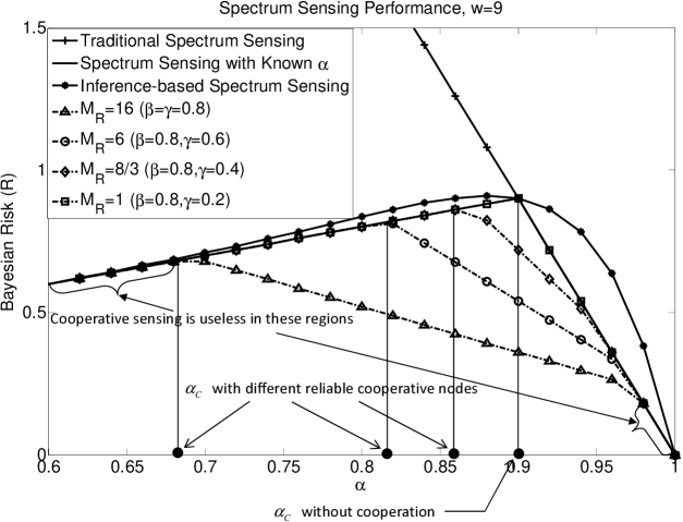
Figure 3: Performance (Bayesian risk) of spectrum sensing schemes with respect to the probability of spectrum availability at CR-Rx $\alpha$. The critical boundary of $\alpha$, $\alpha_{C}$, is represented by $\bullet$ under different sensing schemes .

The performance of spectrum sensing, measured by Bayesian risk (3), is plotted by Bayesian risk versus the probability of spectrum availability at CR-Rx $\alpha$ in Fig. 3. We set the weighting factor $w=9$ ($w$ is defined in (6)) to guarantee the outage probability of CR link less than $0.1$. Larger Bayerian risk represents worse performance because spectrum sensing induces more possibility of collisions at CR-Rx or of losing opportunity to utilize spectrum. We see that traditional spectrum sensing without considering spectrum availability at CR-Rx (i.e. $\mathbf{1}^{Rx}$) has large Bayesian risk when $\alpha$ becomes small because collisions usually occur when CR-Tx determines link availability only by localized spectrum availability at CR-Tx (i.e. $\mathbf{1}^{Tx}$). On the other hand, by considering $\mathbf{1}^{Rx}$ in our general spectrum sensing (5) with known $\alpha$, Bayesian risk decreases when $\alpha$ is less than $0.9$, which is the critical boundary of $\alpha$, $\alpha_{C}$, and CR-Tx is prohibited from forwarding packets to CR-Rx. Therefore, risk occurs due to loss of opportunity to utilize spectrum.

However, in practice, $\alpha$ is unknown and needs to be estimated by Lemma 2. We set observation depth (i.e. duration) $L=15$ and show expected Bayesian risk of inference-based spectrum sensing (5) with respect to observed sequence $\mathbf{1}^{Rx}[n-1],\ldots,\mathbf{1}^{Rx}[n-L]$. The performance degrades around $\alpha_{C}$ and even worse than that of traditional spectrum sensing when $\alpha\geq\alpha_{C}$ because the estimation error may cause the estimated $\alpha$ (4) to across $\alpha_{C}$ and results in different sensing rules; however, it is close to the performance with known $\alpha$. This verifies the effectiveness of inference-based spectrum sensing.

Fig. 3 also shows Bayesian risk of cooperative sensing (8) under different sensing capability of a cooperative node, i.e. reliability $M_{R}$. We assume statistical information $\{\alpha,\beta,\gamma\}$ can be perfectly estimated. The performance curve is composed of three line segments as in (8) and shows performance improvement in the middle segment due to the aid of the cooperative node. However, in the right and the left segments, the cooperative node becomes useless and the performance is equal to that of non-cooperative sensing. In comparison of sensing capability of a cooperative node, the one with larger reliability is expected to have higher correlation between spectrum availability at CR-Rx and the cooperative node (i.e. $\mathbf{1}^{Co}$) and to provide more information about $\mathbf{1}^{Rx}$; therefore, it achieves lower Bayesian risk and lower $\alpha_{C}$ (i.e. larger admissive region). In addition, when $\beta+\gamma=1$ ($\beta=0.8,\gamma=0.2$), $\mathbf{1}^{Rx}$ and $\mathbf{1}^{Co}$ are independent and the performance is identical to that of spectrum sensing with known $\alpha$ in Fig. 3.

VI-A2 Impacts of Correlation between Spectrum Availability at Cooperative Nodes

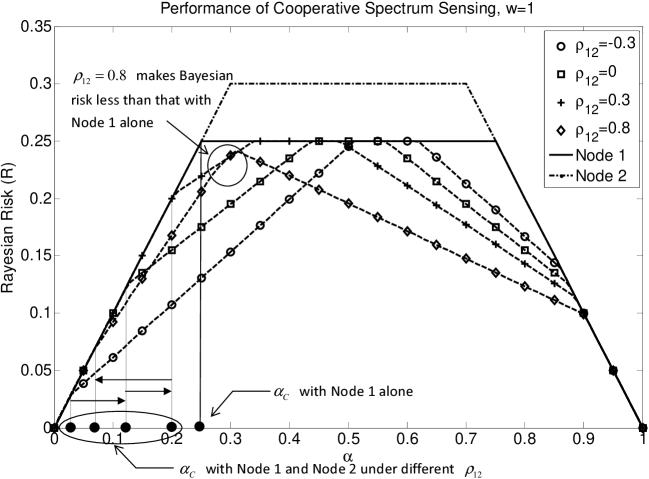
Figure 4: Performance of spectrum sensing with one/two cooperative node(s) with respect to the probability of spectrum availability at CR-Rx $\alpha$. The transition and the value of the critical boundary of $\alpha$, $\alpha_{C}$, under different correlation of Node 1 and Node 2 $\rho_{12}$ is also shown.

We next investigate performance of spectrum sensing with two cooperative nodes with respect to the correlation between spectrum availability at these two nodes (i.e. $\mathbf{1}^{Co}_{1}$ and $\mathbf{1}^{Co}_{2}$) $\rho_{12}$. We set $\beta_{1}=\gamma_{1}=0.75$, $\beta_{2}=\gamma_{2}=0.7$ as the scenario in Proposition 7 and depict Bayesian risk in Fig. 4. Generally speaking, Bayesian risk decreases (increases) as $\rho_{12}$ increases in high (low) $\alpha$. We also observe that $\alpha_{C}$ decreases when number of cooperative nodes increases and $\alpha_{C}$ increases when $\rho_{12}$ increases unless the correlation is high enough. For example, if two cooperative nodes are close in location and $\rho_{12}=0.8$, $\alpha_{C}$ is less than that when $\rho_{12}=0$. It is also interesting to note that there exists a region of $\alpha$ such that the identity of $\mathbf{1}^{Co}_{1}$ and $\mathbf{1}^{Co}_{2}$ instead of $\mathbf{1}^{Co}_{1}$ determines CR link availability as in (29) and Bayesian risk is less than that with $\mathbf{1}^{Co}_{1}$ alone.

The results further suggest trade-off between performance in link layer and network layer when we select cooperative nodes. That is, for one CR link with $\alpha>0.5$ (e.g. CR-Rx is close to CR-Tx or spectrum utilization of PS is low), large $\rho_{12}$ is preferred to achieve low risk. However, from network perspective, to achieve high number of CR links that are admissive to CR-Tx (i.e. to achieve large neighborhood and low $\alpha_{C}$) and thus high throughput of CRN, small $\rho_{12}$ is preferred.

VI-A3 Robust Spectrum Sensing

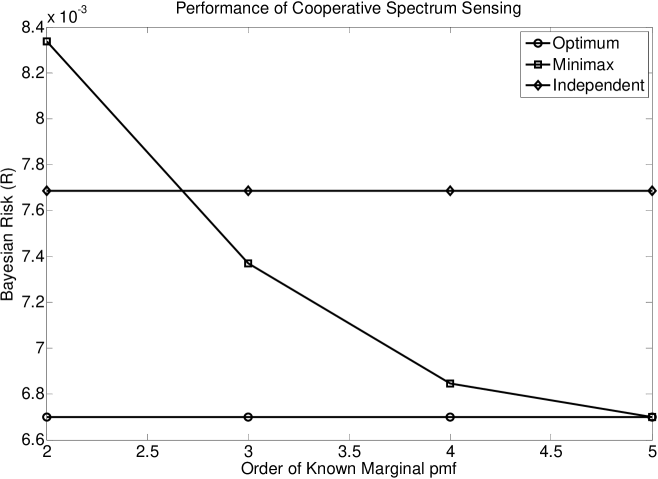
Figure 5: Performance of robust spectrum sensing under different order of known marginal pmf $k$, that is, pmf of $k$ out of six cooperative nodes is available at CR-Tx. The performance is compared to the spectrum sensing with full statistical information and with traditional independence assumption.

For multiple cooperative nodes, with six nodes in our simulation, we show the performance of cooperative spectrum sensing with limited statistical information $\mathbf{Q}^{(s)}_{k,K},s=0,1$ due to limited sensing duration. We first find least-favorable joint pmf $\mathbf{P}^{(s)}_{opt},s=0,1$ by (31) and then compute corresponding Bayesian risk, which is shown in Fig. 5 under different order of known marginal pmf $k$ (i.e. capability of observation). That is, CR-Tx only acquires pmf of $k$ out of six cooperative nodes. The risk is compared to that with the optimum sensing rule (23) and that with assumption of independent spectrum availability (28). Obviously, Bayesian risk decreases and approaches to that in the optimum case as the order of known marginal pmf $k$ increases because more information is acquired to generate $\mathbf{P}^{(s)}_{opt},s=0,1$ closer to the true one $\mathbf{P}^{(s)}_{K},s=0,1$. We observe that when the order $k$ is greater than 3, robust spectrum sensing outperforms the case of traditional independence assumption. Therefore, if CR-Tx would like to select six cooperative nodes, CR-Tx only requires statistical information about spectrum availability among three out of six cooperative nodes, i.e. $\mathbf{Q}^{(s)}_{3,6},s=0,1$, to achieve better performance than the case according to reliability criterion.

VI-B Neighborhood of CR-Tx

VI-B1 Without Obstacles

In Fig. 6, we illustrate neighborhood of CR-Tx (”$+$” in the figure) without blocking. The neighborhood boundary with/without a cooperative node (”$\circ$” in the figure) is depicted by a thick and a thin line respectively. The parameters are set as follows: $\mu_{0}=0$, $\sigma_{0}^{2}=1$, $\sigma_{S}^{2}=8$, $K_{0}=10$, $a=3$, $L_{0}=3$, $\tau_{Tx}=\tau_{Co}=3$, and $\Pr(\mathbf{1}^{PS}=1)=0.6$.

In Fig. 6(a), PS (”$\ast$” in the figure) is placed near to CR-Tx ($(0.7,0)$). We observe that CR-Tx almost perfectly detects the state of PS, i.e., $\Pr(\mathbf{1}^{Tx}=1|\mathbf{1}^{PS}=1)\approx 1$ and $\Pr(\mathbf{1}^{Tx}=1|\mathbf{1}^{PS}=0)\approx 0$, and $\alpha\approx\Pr(\mathbf{1}^{Rx}=1|\mathbf{1}^{Tx}=1,\mathbf{1}^{PS}=1)$ by (32). Therefore, neighborhood of CR-Tx approaches to its coverage and the cooperative node is not necessary in this case from a viewpoint of network operation. However, when PS is apart from CR-Tx ($(1.7,0)$) as we shown in Fig. 1, the neighborhood at PS side shrinks and is no longer circularly shaped because PS is hidden to CR-Tx and hence probability of collision at CR-Rx increases when $\mathbf{1}^{PS}=0$. Fig. 6(b)$\sim$(d) illustrate the neighborhood under different locations of the cooperative node. We observe that neighborhood area decreases when the cooperative node moves away from PS and there even exists a region where cooperative sensing can not help. Therefore, the cooperative node in Fig. 6(b) is the best among these three nodes according to maximum neighborhood area criterion in Proposition 10.

We present an example of existence of unidirectional link in CRN. In Fig. 6(b), assume one CR is located at $(1,0)$. Obviously, the CR-Tx is not connective to the CR and therefore is prohibited from forwarding packets to the CR. However, by Fig. 6(a), the CR is connective to CR-Tx, which makes the link unidirectional (only from the CR to CR-Tx). As Proposition 9, this also shows asymmetric connective relation even under rather ideal radio propagation. With the aid of a cooperative node located at $(0.4,0.3)$, the link returns to a bidirectional link.

VI-B2 With Obstacles

Alternatively, we consider effects of shadowing due to blocking, as we illustrated in Fig. 2. We set shadowing parameters $b_{Tx}=25$ and parameter of obstacle size $\kappa=0.3$ and $0.7$ in Fig. 7(a)(b) and Fig. 7(c)(d) respectively. We observe that small obstacles size (i.e. small $\kappa$) can result in more substantial shrink of the neighborhood, compared to large obstacles size (i.e. large $\kappa$). The reason is: if $\kappa$ is small, only a small region around CR-Tx falls in deep shadowing and the state of PS can be successfully detected outside that region. Therefore, this leads to high probability of collision at CR-Rx as $\mathbf{1}^{PS}=0$. On the other hand, if $\kappa$ is large, CRs are likely separated from PS by obstacles, which results in large ”distance” between CR and PS. Here, ”distance” is measured by received signal power [16][36]. In comparison of the capability of a cooperative node, the one in small $\kappa$ has good capability to recover the neighborhood to its coverage even when the node is at opposite side of PS. However, for large $\kappa$, the cooperative node may also be in deep shadowing and becomes useless to recover neighborhood of CR-Tx.

VII Conclusion

In this paper, we showed that CR link availability should be determined by spectrum availability at both CR-Tx and CR-Rx, which may not be identical due to hidden terminal problem (Fig. 1 and 2). In order to fundamentally explore the spectrum sensing at link level and its impacts on network operation, we established an indicator model of CR link availability and applied statistical inference to predict/estimate unknown spectrum availability at CR-Tx due to no centralized coordinator nor information exchange between CR-Tx and CR-Rx in advance. We therefore expressed conditions for CR-Tx to forward packets to CR-Rx under guaranteed outage probability. These conditions, along with physical channel models, define neighborhood of CR-Tx, which is no longer circularly shaped as coverage. This results in asymmetric or even unidirectional links in CRN, as we illustrated in Section VI. The impairment of CR links can be alleviated via cooperative scheme. Therefore, spectrum sensing capability determines network topology and thus throughput of CRN. Several factors with impacts on spectrum sensing are analyzed, including:

1. Correlation of spectrum availability at cooperative nodes

2. Capability of observation at CR-Tx (i.e. available statistical information at CR-Rx)

3. Locations of cooperative nodes and environment (i.e. obstacles)

Furthermore, limits of cooperative scheme were also addressed in link level and network level. In addition, to measure sensing capability and then to select cooperative nodes is an important issue because we would like to minimize information exchange to increase spectrum utilization. Criterions from link level (maximum reliability or minimum Bayesian risk) and network level (maximum neighborhood area) perspectives were accordingly proposed. We numerically demonstrated existence of trade-off in designing systems in different layers. In addition, robust spectrum sensing was proposed to deal with local and partial information due to no centralized coordination and limited sensing duration in CRN. More useful results in CRN extended from this research can be expected in future works.

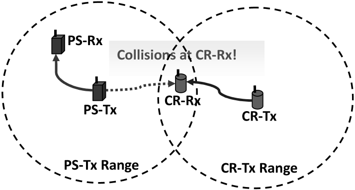
Figure 1: Hidden terminal problem. CR-Rx lies in the middle of CR-Tx and PS-Tx and PS-Tx is hidden to CR-Tx.

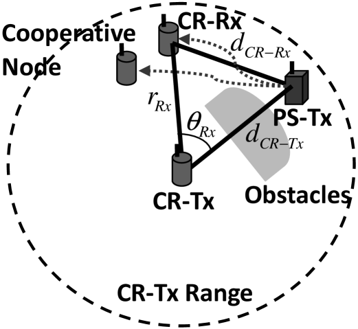
Figure 2: Activities of PS-Tx is blocked by obstacles to CR-Tx but not to CR-Rx.

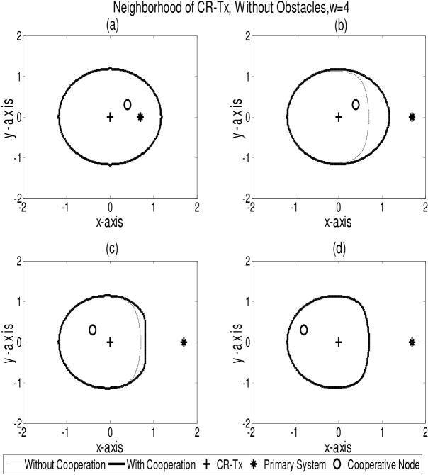
Figure 6: Neighborhood of CR-Tx without obstacles. CR-Tx can only be allowed forwarding to CR-Rx located within the bounded region.

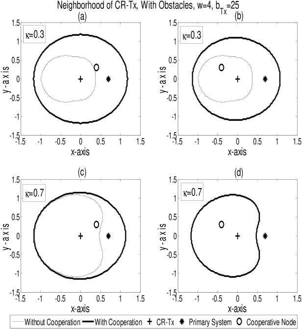
Figure 7: Neighborhood of CR-Tx with obstacles. Effects of small ($\kappa=0.3$ in (a)(b)) and large ($\kappa=0.7$ in (c)(d)) obstacles are compared.

References

• [1] J. Mitola III, ”Cognitive radio: an integrated agent architecture for software defined radio,” Ph.D. dissertation, Royal institute of Technology (KTH), Stockholm, Sweden, 2000.
• [2] FCC Spectrum Policy Task Force, ”FCC report of the spectrum efficiency working group,” Nov. 2002, http://www.fcc.gov/sptf/files/SEWGFinalReport_1.pdf.
• [3] S. Haykin, ”Cognitive radio: brain-empowered wireless communications,” IEEE Journal on Selected Areas in Communications, vol. 23, pp. 201-220, Feb. 2005.
• [4] A. Ghasemi and E. S. Sousa, ”Spectrum sensing in cognitive radio networks: requirements, challenges and design trade-offs,” IEEE Communications Magazine, vol. 46, no. 4, pp. 32-39, Apr. 2008.
• [5] J. Ma, G. Y. Li, and B. H. Juang, ”Signal processing in cognitive radio,” Proceeding of the IEEE, vol. 97, no. 5, May 2009.
• [6] T. Yucek and H. Arslan, ”A survey of spectrum sensing algorithms for cognitive radio applications,” IEEE Communications Surveys $\&$ Tutorials, vol. 11, no. 1, First Quater 2009.
• [7] D. Cabric, S. M. Mishra, and R. W. Broderson, ”Implementation issues in spectrum sensing for cognitive radios,” IEEE Proc. Signals, Systems, and Computers, pp. 772-776, Nov. 2004.
• [8] A. Sahai, N. Hoven, and R. Tandra, ”Some fundamental limits on cognitive radio,” in Proc. Allerton Conf. on Commun., Control, and Computing, Oct. 2004.
• [9] F. F. Digham, M. S. Alouini, and M. K. Simon, ”On the energy detection of unknown signals over fading channels,” IEEE Proc. ICC, pp. 3575-3579, May 2003.
• [10] Y. M. Kim, G. Zheng, S. H. Sohn, and J. M. Kim, ”An alternative energy detection using sliding window for cognitive radio system,” IEEE Proc. ICACT, pp. 481-485, Feb. 2008.
• [11] J. Zhu, Z. Xu, F. Wang, B. Huang, and B. Zhang, ”Double threshold energy detection of cooperative spectrum sensing in cognitive radio,” IEEE Proc. CrownCom, pp. 1-5, May 2008.
• [12] B. Farhang-Boroujeny, ”Filter bank spectrum sensing for cognitive radios,” IEEE Transactions on Signal Processing, vol. 56, no. 5, pp. 1801-1811, May 2008.
• [13] F. Penna, C. Pastrone, M. A. Spirito, and R. Garello, ”Energy detection spectrum sensing with discontinuous primary user signal,” IEEE Proc. ICC, Jun. 2009.
• [14] W. A. Gardner, ”Signal interception: A unifying theoretical framework for feature detection,” IEEE Transactions on Communications, vol. 38, pp. 897-906, Aug. 1988.
• [15] W. A. Gardner, ”Exploitation of spectral redundency in cyclostationary signals,” IEEE Signal Processing Magazine, vol.8, pp. 14-36, Apr. 1991.
• [16] S. Y. Tu, K. C. Chen, and R. Prasad, ”Spectrum sensing of OFDMA systems for cognitive radio networks,” to appear in the IEEE Transactions on Vehicular Technology.
• [17] K. Kim, I. A. Akbar, K. K. Bae, J-S Um, C. M. Spooner, and J. H. Reed, ”Cyclostationary approaches to signal detection and classification in cognitive radio,” IEEE Proc. DySPAN, pp. 212-215, Apr. 2007.
• [18] H. Guo, H. Hu, and Y. Yang, ”Cyclostaionary signatures in OFDM-based cognitive radios with cyclic delay diversity,” Proc. IEEE ICC, Jun. 2009.
• [19] D. Cabric, A. Tkachenko, and R. W. Brodersen, ”Spectrum sensing measurements of pilot, energy, and collaborative detection,” IEEE Proc. MILCOM, pp. 1-7, Oct, 2006.
• [20] Y. Zeng and Y. C. Liang, ”Covariance based signal detections for cognitive radio,” IEEE Proc. DySPAN, pp. 202-207, Apr. 2007.
• [21] Y. Zeng and Y. C. Liang, ”Maximum-minimum eigenvalue detection for cognitive radio,” IEEE Proc. PIMRC, pp. 1-5, Sep. 2007.
• [22] Y. Zeng and Y. C. Liang, ”Spectrum-sensing algorithms for cognitive radio based on statistical covariances,” IEEE Transactions on Vehicular Technology, vol. 58, no. 4, May 2009.
• [23] Q. T. Zhang, ”Advanced detection techniques for cognitive radio,” IEEE Proc. ICC, Jun. 2009.
• [24] B. Zayen, A. Hayar, and K. Kansanen, ”Blind spectrum sensing for cognitive radio based on signal space dimension estimation,” IEEE Proc. ICC, Jun. 2009.
• [25] Z. Tian and G. B. Gianakis, ”A wavelet approach to wideband spectrum sensing for cognitive radios,” IEEE Proc. CROWNCOM, pp. 1-5, Jun. 2006.
• [26] J. Unnikrishnan, and V. V. Veeravalli, ”Cooperative sensing for primary detection in cognitive radio,” IEEE Journal on Selected Topics in Signal Processing, vol. 2, no. 1, pp. 18-27, Feb. 2008.
• [27] Z. Quan, S. Cui, and A. H. Sayed, ”Optimal linear cooperation for spectrum sensing in cognitive radio networks,” IEEE Journal on Selected Topics in Signal Processing, vol. 2, no. 1, pp. 28-40, Feb. 2008.
• [28] G. Ganesan, and J. Li, ”Cooperative spectrum sensing in cognitive radio, Part I: Two-user networks,” IEEE Transactions on Wireless Communications, vol. 6, no. 6, pp. 2204-2213, June 2007.
• [29] G. Ganesan, and J. Li, ”Cooperative spectrum sensing in cognitive radio, Part II: Multiuser networks,” IEEE Transactions on Wireless Communications, vol. 6, no. 6, pp. 2214-2222, June 2007.
• [30] A. Ghasemi and E. S. Sousa, ”Collaborative spectrum sensing for oppotunistic access in fading environments,” IEEE Proc. DYSPAN, pp. 131-136, Jun. 2005.
• [31] Z. Quan, S. Cui, A. H. Sayed, and H. V. Poor, ”Optimal multiband joint detection for spectrum sensing in cognitive radio networks,” IEEE Transactions on Signal Processing, vol. 57, no. 3, pp. 1128-1140, Mar. 2009.
• [32] S. M. Mishra, A. Sahai, and R. W. Broderson, ”Cooperative sensing among cognitive radios,” IEEE Proc. ICC, pp. 1658-1663, Jun. 2006.
• [33] S. A. Jafar and S. Srinivasa, ”Capacity limits of cognitive radio with distributed and dynamics spectral activity,” IEEE Journal on Selected Areas in Communications, vol. 25, no. 3, pp. 529-537, Apr. 2007.
• [34] S. Srinivasa and S. A. Jafar, ”The throughput potential of cognitive radio: A theoretical perspective,” IEEE Communications Magazine, vol. 45, no. 5, pp. 73-79, May 2007.
• [35] K. Xu, M. Gerla, and S. Bae, ”How effective is the IEEE 802.11 RTS/CTS handshake in ad hoc networks?” IEEE Proc. GLOBECOM, pp. 72-76, Nov. 2002.
• [36] K. C. Chen, L. H. Kung, D. Shiung, R. Prasad, and S. Chen, ”Self-organizing terminal architecture for cognitive radio networks,” The 10th International Symposium on Wireless Personal Multimedia Communications, pp. 926-931, Dec. 2007.
• [37] R. Viswanathan and V. Aalo, ”On counting rules in distributed detection,” IEEE Transactions on Acoustics, Speech and Signal Processing, vol. 37, no. 5, pp. 772-775, May 1989.
• [38] A. Ghasemi and E. S. Sousa, ”Interference aggregation in spectrum sensing cognitive wireless networks,” IEEE Journal on Selected Topics in Signal Processing, vol. 2, no. 1, pp. 41-56, Feb. 2008.
• [39] C. K. Yu and K. C. Chen, ”Radio resource tomography of cognitive radio networks,” IEEE Proc. VTC, Apr. 2009.
• [40] C. K. Yu, K. C. Chen, and S. M. Cheng, ”Cognitive radio network tomography,” submitted to the IEEE Transactions on Vehicular Technology.
• [41] S. Boyd and L. Vandenberghe, Convex optimization, Cambridge University Press, 2004.
• [42] H. V. Poor, An introduction to signal detection and estimation, Springer-Verlag, 1994.
• [43] G. Cacella and R. L. Berger, Statistical inference, Duxbury, 2002.
• [44] R. W. Thomas, R. S. Komali, A. B. MacKenzie, and L. A. DaSilva, ”Joint power and channel minimization in topology control: A congnitive network approach,” IEEE Proc. ICC, pp. 6538-6543, Jun. 2007.
• [45] T. Chen, H. Zhang, G. M. Maggio, and I. Chlamtac, ”Topolog management in CogMesh: A cluster-based cognitive radio mesh network,” IEEE Proc. ICC, pp. 6516-6521, Jun. 2007.
• [46] K. C. Chen, Y. C. Peng, B. K. Centin, N. Prasad, J. Wang, and S. Y. Lee, ”Routing of opportunistic links in cognitive radio networks,” to appear in the Wiley Wireless Communicatioins and Mobile Computing.
• [47] K. C. Chen and R. Prasad, Cognitive Radio Networks, Wiley, 2009.
Refer to caption