Spectroscopically- and spatially-resolved optical line emission in the Superantennae (IRAS 19254-7245)

Abstract

We present VIMOS integral field spectroscopic observations of the ultraluminous infrared galaxy (ULIRG) pair IRAS 19254-7245 (the Superantennae). We resolve H$\alpha$, [N II], [O I], and [S II] emission both spatially and spectroscopically and separate the emission into multiple velocity components. We identify spectral line emission characteristic of star formation associated with both galaxies, broad spectral line emission from the nucleus of the southern progenitor, and potential outflows with shock-excited spectral features near both nuclei. We estimate that $~{}\hbox to0.0pt{$<$\hss}{\lower 4.30554pt\hbox{$\sim$}}10$% of the 24 $\mu$m flux density originates from star formation, implying that most of the 24 $\mu$m emission originates from the AGN in the southern nucleus. We also measure a gas consumption time of $\sim 1$ Gyr, which is consistent with other measurements of ULIRGs.

1 Introduction

We are undertaking an integral field spectroscopic survey of a volume-limited sample of 18 ultraluminous infrared galaxies (ULIRGs; galaxies where $L_{IR}>10^{12}L_{\odot}$) with the Visible Multi-Object Spectrograph (VIMOS; LeFevre et al., 2003) at the Very Large Telescope. We have two main scientific goals. First, we want to study gas inflow and outflow in ULIRGs, with particular emphasis on the detection of starburst-driven superwinds or AGN-driven jets, and determine whether these outflows may be part of a feedback mechanism that inhibits star formation. Second, we want to examine gas excitation mechanisms within these galaxies and determine whether AGN or star formation dominate the energetics of ULIRGs. The results from this survey can be applied to understanding the dynamics and rest-frame optical spectra of both nearby and more distant ULIRGs, especially in light of recently published integral field spectroscopic observation of infrared- and submillimetre-luminous $z>1$ objects (e.g. Swinbank et al., 2005, 2006).

We present here the first results from this survey: VIMOS integral field spectroscopic observations of IRAS 19254-7245 (the Superantennae). The object, which has two distinct nuclei and two tidal tails that extend over hundreds of kpc (Mirabel et al., 1991), has been the subject of many detailed studies. The southern nucleus contains an AGN, as shown by studies at multiple wavelengths (Vanzi et al., 2002; Charmandaris et al., 2002; Braito et al., 2003; Berta et al., 2003; Reunanen et al., 2007), but the northern nucleus appears to be completely dominated by star formation (Braito et al., 2003; Berta et al., 2003). Some evidence has been given for the presence of several distinct dynamical components within the inner arcmin of the galaxy, including a broad line component (full-width half-maximum (FWHM) $\sim 2000$-2500 km s^-1) associated with the southern nucleus, narrower components (FWHM $<500$ km s^-1) associated with the progenitor discs, and some high-velocity clouds (Vanzi et al., 2002; Reunanen et al., 2007). However, the previous optical studies have been mainly single slit spectra that have lacked spatial information, and previous near-infrared integral field spectroscopic observations covered only an $8\times 8$ arcsec region that does not include all the emission from the southern disc. The VIMOS data that we present here, which covers the central $35\times 35$ arcsec, allows us to resolve optical line emission both spatially and spectroscopically, so we can clearly discern the AGN, star-forming regions, and other structures within both galaxies. We used this galaxy to test many of the analysis methods that will be applied to the sample as a whole. The spectral line emission in this galaxy pair was detected at significantly larger radii and the line-emitting structures are more complex than most other sample galaxies, which is why we have focused on it for this first paper.

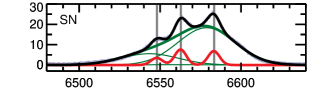
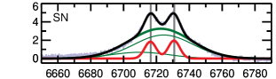
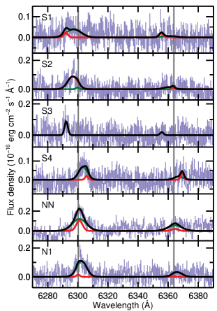
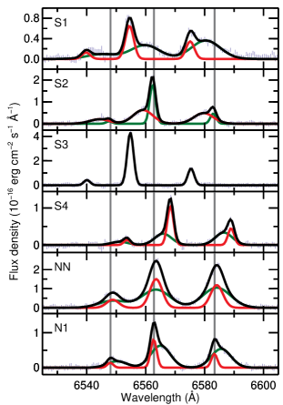
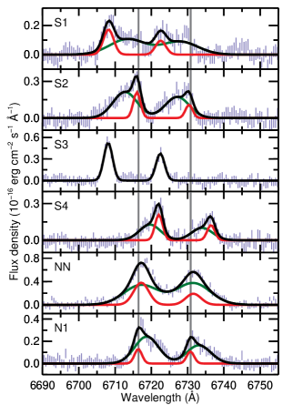
Figure 1: Subsections of the spectra extracted from different regions drawn as blue error bars, with the best fitting models overplotted as solid black lines. When two velocity components are fit to the data, component 1 is shown in red and component 2 is shown in green. For region SN, the individual spectral lines for the broader velocity component are shown as thin green lines. Line centers for the [O I] 6300 and 6364 Å lines, the [N II] 6548 and 6583 Å lines, the 6563 Å H$\alpha$ line, and the 6716 and 6731 Å lines are overplotted as grey lines. Parameters from these fits are given in Table 1. The spectra for region SN are shown over a broader wavelength range because the lines are broader than in other regions.

Table 1: Parameters for line fits for regions in Figure 3

	H$\alpha$	H$\alpha$	Flux (erg cm-2 s-1)
Region	velocitya	line widthb	[O I]	H$\alpha$	[N II]	[S II]	[S II]
	(km s-1)	(km s-1)	6300 Å	6563 Å	6583 Å	6716 Å	6731 Å
	$-7.9\pm 0.3$	$379.8\pm 0.9$	$5.4\pm 0.3$	$67.8\pm 0.3$	$60.0\pm 0.3$	$16.27\pm 0.16$	$17.32\pm 0.17$
SN	$-162.9\pm 1.7$	$1851.3\pm 1.5$	$107.3\pm 0.25$	$59\pm 3$	$761.9\pm 1.5$	$53.9\pm 0.6$	$97.9\pm 0.6$
	$-379\pm 4$	$153\pm 7$	$0.08\pm 0.07$	$2.3\pm 0.2$	$1.23\pm 0.14$	$0.61\pm 0.09$	$0.34\pm 0.08$
S1	$-137\pm 14$	$529\pm 17$	$0.48\pm 0.16$	$3.3\pm 0.2$	$4.5\pm 0.3$	$1.31\pm 0.17$	$1.10\pm 0.16$
	$-21\pm 5$	$108\pm 5$	$0.03\pm 0.05$	$4.5\pm 0.4$	$1.15\pm 0.15$	$0.53\pm 0.10$	$0.27\pm 0.08$
S2	$-170\pm 11$	$358\pm 9$	$0.74\pm 0.15$	$5.2\pm 0.4$	$4.0\pm 0.2$	$1.78\pm 0.16$	$1.44\pm 0.15$
S3	$-366.3\pm 0.7$	$117.3\pm 0.7$	$0.24\pm 0.08$	$11.85\pm 0.14$	$3.75\pm 0.07$	$1.6\pm 0.3$	$1.13\pm 0.19$
	$256\pm 6$	$114\pm 6$	$0.05\pm 0.06$	$2.8\pm 0.4$	$1.2\pm 0.2$	$0.55\pm 0.13$	$0.33\pm 0.09$
S4	$140\pm 20$	$311\pm 16$	$0.50\pm 0.15$	$2.2\pm 0.5$	$2.4\pm 0.3$	$0.9\pm 0.2$	$0.73\pm 0.15$
	$34\pm 3$	$226\pm 13$	$0.5\pm 0.2$	$7.9\pm 1.4$	$6.3\pm 1.3$	$2.0\pm 0.5$	$1.0\pm 0.3$
NN	$33\pm 4$	$510\pm 20$	$1.4\pm 0.4$	$11\pm 3$	$12\pm 3$	$4.0\pm 0.9$	$4.4\pm 0.7$
	$-4\pm 6$	$110\pm 8$	$0.04\pm 0.13$	$2.1\pm 0.4$	$1.0\pm 0.2$	$0.33\pm 0.10$	$0.28\pm 0.09$
N1	$102\pm 10$	$356\pm 8$	$0.90\pm 0.15$	$5.2\pm 0.5$	$4.5\pm 0.3$	$2.01\pm 0.18$	$1.36\pm 0.15$

^a These are calculated relative to a central velocity of 17950 km s^-1. Negative velocities correspond to blueshifted lines.
^b These are based on the FWHM of the lines.

2 Observations, data reduction

Observations were performed with the VIMOS integral field unit at the Very Large Telescope on 2007 October 9. The data were taken using the HR red grism (6300-8700 Å), which has a spectral resolution of 3100, and a plate scale of 0.67 arcsec for each fibre that gave a field of view of $27\times 27$ arcsec for each pointing. The seeing during the observations was $\sim 0.7$ arcsec. Spectra were measured in five pointings offset from each other by 5 arcsec, which provided redundancy within the central region and ensures the availability of blank sky for background measurements. This strategy is used for all galaxies in the ULIRG survey.

The VIMOS data reduction pipeline produces calibrated spectra that show the spectra measured for each fibre. The data from each pointing are stored in four files that contain the spectra from the four quadrants of the integral field unit. We used these pipeline-processed data for our analysis, but additional processing was needed to transform the spectra into a data cube. First, for each pointing and for each quadrant, we identified fibres that measured background emission by integrating the spectra and using an iterative process to remove fibres with high continuum signals, which would indicate the presence of emission from the target. Median background spectra for each quadrant and each pointing were determined using these background fibres, and these background spectra were subtracted from the data. Following this, the spectra from each pointing were mapped into individual spectral cubes, and then the cubes were median combined to produce the final spectral cube.

3 Spectral line fitting and analysis

Before measuring spectral line emission, we corrected the data for redshift using a velocity of $\sim 17950$ km s^-1, which was estimated empirically to be the approximate velocity of narrow-line emission from the southern nucleus, and we subtracted a continuum determined by fitting a line through the data between 6100-6200 Å and between 6800-7000 Å in the rest frame. We then fit Gaussian functions to the H$\alpha$, [O I], [N II], and [S II] lines within each spectrum in the data cube. We forced the fits to treat the offset between adjacent spectral features (i.e. adjacent [O I] lines, adjacent [S II], or lines near H$\alpha$) as constants. We generally determined whether to fit one or two velocity components by visually inspecting the lines for features such as skewed line profiles or double-peaked structures that would indicate that two velocity components are present, but we also decided to fit two velocity components to the data when the two component fit produced a lower reduced $\chi^{2}$. When we fit one velocity component, we used the same line widths for adjacent lines. When we fit two velocity components to the data, we fit both simultaneously. To reduce the uncertainties in the line fits where two velocity components were present, we performed fits to all spectral features between 6200-6800 Å where the offsets among all spectral lines were treated as constants and where the corresponding line widths for each velocity component were treated as equal. We also forced all line fluxes to be positive in all fits.

Examples of spectral line fits are shown in Figure 1, with parameters for the best fit lines given in Table 1. Each spectrum was extracted from multiple spatial pixels for the analysis later in this section, but similar fits were applied to the spectra for single spatial pixels. We also used three of these regions to show in Figure 2 examples of the robustness of the fits to the H$\alpha$ line. Region S3 is an example or where we observed spectral line emission from a single velocity component; we demonstrate with this profile that the spectral line is fit better by a Gaussian function than by a Lorentz function. Region N1 is an example of where the spectral lines are significantly skewed and must be fit by two Gaussian functions. Region NN is a special case found in only one location in the object where the lines exhibit extra kurtosis. When we fit one Gaussian function, we saw that the lines had both high central peaks and broad wings when compared to the fit, as shown by the high positive residuals for the H$\alpha$ line fit in Figure 2. The line is better fit by either a single Lorentz function or by two Gaussian functions with similar central wavelengths. However, the emission from region N1 immediately to the west of NN consists of skewed lines with two velocity components that have line widths and line ratios similar to those in the two Gaussian component fit to NN. This suggest that the line profiles for NN should be modeled as two Gaussian components and not one Lorentz component.

The results from the fits to each spatial pixel were then used to produce maps of the parameters, as shown in Figure 3. Additionally, Figure 4 shows how the velocities and line widths vary across vertical and horizontal lines that were placed so as to cover locations of interest with two velocity components. Component 1 contains almost all of the emission from locations with only a single line component and most of the narrower line emission in locations with two line components. Component 2 generally contains broader spectral line emission. In the southeastern HII region, however, we found that the broader spectral line component had velocities that were closer to the velocities traced by the narrow line component in adjacent pixels and that the velocities of the narrow component were sharply different from component 1 in adjacent pixels, as seen in Figure 4. We therefore shifted the narrower line emission for these locations into component 2 and the broader line emission into component 1. We also found six pixels along the southern or western edge of the detected region where either a single line component or a narrower line component had velocities closer to that for the broader line component in adjacent pixels, and so the narrower or single line component was shifted to component 2 in these cases as well.

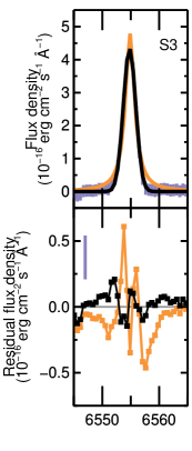
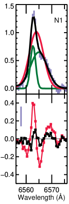
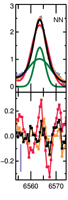
Figure 2: The top panels show spectra for the regions around the H$\alpha$ line extracted from the regions in Figure 3. The data are shown as blue error bars. The best fitting model (one Gaussian function for S3 and two Gaussian functions for N1 and NN) are shown in black. Individual components of the two Gaussian function models are shown in green. Alternate single Lorentz functions for regions S3 and NN are shown in orange (although the orange lines are mostly overlapped by the black lines); alternative single Gaussian functions for regions N1 and NN are shown in red. The bottom panels show the residuals from the best fitting models in black and the residuals from the alternate models in red or orange, with the individual data points shown as squares and the typical size of the error bars shown as a blue line on the left side of the panels.

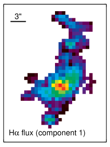
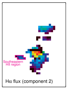
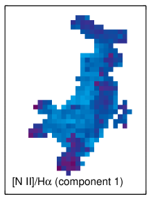
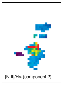
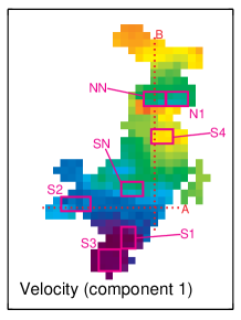
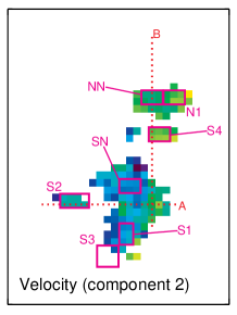
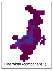
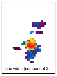
Figure 3: Images of the H$\alpha$ flux, the [N II]/H$\alpha$ flux ratio, the H$\alpha$ velocity, and the H$\alpha$ line widths for the inner $20\times 26$ arcsec of the Superantennae. The kinematic structures have been divided into two components, with the broader spectral lines generally placed in the second component; see the text for details. The objects in each frame may not necessarily be physically associated. North is up and east is left in each image, and the angular scale is shown in the H$\alpha$ flux image for the first component. The magenta regions in the velocity images are the locations for which spectra are displayed in Figure 1. The red dotted lines show the locations with velocities and line widths plotted in Figure 4.

We can see two rotating progenitors and a couple of H$\alpha$-bright knots in component 1 in Figure 3. In component 2, we can see broad (FWHM $\sim 1850$ km s^-1) spectral line emission from the nucleus, a broad arc to the southeast of the nucleus, and a few other regions in both progenitors. The velocity maps and Figure 4 clearly show that the two progenitors are rotating in the same direction.

The individual spectra shown in Figure 1 are useful for understanding the nature of the different regions of the galaxy. In the following discussion, we use the spectral line diagnostics presented by Kewley et al. (2006) to determine whether the spectral line emission is consistent with star formation or AGN-like emission, although the usefulness of these diagnostics is limited without additional measurements of H$\beta$ and [O III] (5007 Å) fluxes. We treat locations where log([OI] (6300 Å)/H$\alpha$) $<$ -1.0, log([NII] (6583 Å)/H$\alpha$) $<$ 0 and log([SII] (6716,31 Å)/H$\alpha$) $<$ -0.2 as being dominated by photoionisation from star formation, whereas regions with higher line ratios are treated as having AGN-like emission. The southern nucleus (SN) contains both broader and narrower emission line components. The narrow component probably originates from the progenitor disc remnant, and the spectral line ratios are consistent with star formation. The broader component is consistent with AGN activity. In particular, the H$\alpha$ emission is very weak compared to other spectral features, most notably seen in the map of the [N II]/H$\alpha$ ratio, indicating that the gas is ionised by a hard radiation field. This is consistent with results for Pa$\alpha$ found by Reunanen et al. (2007). S1 contains both a narrower component associated with the disc remnant and a broader component that is part of the arc extending from the southern nucleus. The line ratios of the broader component are consistent with AGN-like emission, which implies that this extension is a shock similar to those seen in other ULIRGs by Monreal-Ibero et al. (2006). The apparent physical connection to the southern nucleus, the smooth changes in velocity from the southern nucleus to the arc, and the uniform [N II]/H$\alpha$ ratio across the arc imply that it is gas ejected from the southern nucleus. However, the orientation and motion of the arc relative to the rotation of the southern disc remnant imply that it could be a tidal feature. The broader component in S2 is associated with the southern disc remnant, while the narrower component is associated with a cloud moving at a higher velocity. Both components in region S2 have line ratios that are consistent with photoionisation. The spectrum of the region in S3 is consistent with star formation. The spectrum of S4 contains two components, and the broader component is consistent with AGN emission. In NN and N1, the line ratios of the narrower components are like HII emission, but the broader components are AGN-like. While the broader components of NN and N1 may be associated with ejecta from the southern nucleus or with material stripped or ejected from the southern disc remnant, its location and velocity imply that the emission originates from gas ejected from the northern disc remnant.

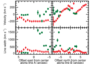
Figure 4: Velocities and line widths for component 1 (as red diamonds) and component 2 (as green squares) for the locations shown by the dotted lines in Figure 3.

Based on the application of the diagnostics from Kewley et al. (2006), component 1 and the southeastern HII region in component 2 (outlined in magenta in Figure 3) appear to trace all of the star formation. The total H$\alpha$ flux from star formation as traced by these components is $(3.52\pm 0.02)\times 10^{-14}$ erg s^-1 cm^-2, or $\sim 70$% of the total H$\alpha$ flux from the galaxy. To understand the relative contribution of star formation to the 24 $\mu$m flux density, we can use extinction measurements from the literature and the H$\alpha$ flux in

$$f_{H\alpha}e^{0.812A_{V}}=f_{H\alpha}+0.022\frac{c}{24\mu m}f_{24\mu m}$$ (1)

(adapted from Zhu et al. (2008)) to estimate the 24 $\mu$m flux density from star formation. In this equation, $f_{H\alpha}$ is the measured H$\alpha$ flux, $f_{H\alpha}e^{0.812A_{V}}$ represents the extinction-corrected H$\alpha$ flux, and $f_{24\mu m}$ is the 24 $\mu$m flux density. Although similar equations have been published for individual HII regions within galaxies, the Zhu et al. (2008) version is the only one currently published that has been calibrated for use on global flux measurements, and given that extreme starbursts and AGN with $L_{IR}$ up to $10^{12}$ L_⊙ were included in their analysis, their relation should be applicable to this galaxy. The extinction function of Savage & Mathis (1979) with $R=3.1$ was used to derive the extinction correction term on the left side of the equation. The $A_{V}$ measured in the southern nucleus by Vanzi et al. (2002) and Berta et al. (2003) using single-slit spectra is $\sim 3.1$. Assuming that this extinction applies to all star-forming regions and that the extinction is intrinsic to the source itself, we estimate the 24 $\mu$m flux density from star-forming regions to be $\sim 0.15$ Jy. In contrast, the total 25 $\mu$m flux density measured by IRAS is $1.24\pm 0.06$ Jy (Moshir et al., 1989). We tentatively conclude that $~{}\hbox to0.0pt{$>$\hss}{\lower 4.30554pt\hbox{$\sim$}}90$% of the 24 $\mu$m flux originates from something other than star formation; the AGN in the southern nucleus is the most likely source of this emission.

Our results are consistent with the spectral energy distribution (SED) modelling by Berta et al. (2003), which predicts that the AGN is the dominant source of 25 $\mu$m emission in the Superantennae. While Farrah et al. (2003) found using SED template fitting that AGN may be the primary source of 25 $\mu$m emission in ULIRGs in general, we disagree with their conclusions that the Superantennae SED can be explained entirely by star formation. The starburst template that they used does not accurately describe the Superantennae data between 10-100 $\mu$m, so it may be an inaccurate description of the 24 $\mu$m flux density. While the 24 $\mu$m flux density may be dominated by an AGN, star formation may represent approximately half of 1-1000 $\mu$m flux, and that starburst emission may dominate the far-infrared emission from the Superantennae, as predicted by Berta et al. (2003). Our results rely on the assumption that the kinematic components that we have identified are the only locations with star formation and that the extinction across the star-forming regions in this galaxy is not variable and accurately represented by $A_{V}\simeq 3.1$. Berta et al. (2003) found that extinction was lower in the outer regions of the galaxy, which could reduce the estimated 24 $\mu$m flux density from star formation.

Using the extinction-corrected H$\alpha$ flux for star-forming regions, a distance of 245 Mpc (calculated using a velocity of 17950 km s^-1 and $H_{0}$ of 73 km s^-1 Mpc^-1), and the conversion of H$\alpha$ flux to star formation rate given by Kennicutt (1998), we estimate the star formation rate to be 25 M_⊙ yr^-1. The total molecular gas mass has been measured to be $1.9-3.0\times 10^{10}$ M_⊙ (Mirabel et al., 1990; Vanzi et al., 2002), which would imply a gas consumption time of $\sim 1$ Gyr. While this gas consumption time does not account for gas recycling, it is still indicative of the efficiency of star formation. This is slightly high but still consistent with the “few times $10^{8}$ yr” gas consumption times estimated for ULIRGs using star formation rates derived from far-infrared data (Tacconi et al., 2006), but, as expected, it is lower than the $\sim 3$ Gyr gas consumption times measured for normal spiral galaxies (Kennicutt et al., 1994).

References

- Braito et al. (2003) Braito, V., et al., 2003, A&A, 398, 107
- Berta et al. (2003) Berta, S. Fritz, J., Franceschini, A., Bressan, A., & Pernechele, C., 2003, A&A, 403, 119
- Charmandaris et al. (2002) Charmandaris, V., et al., 2002, A&A, 391, 429
- Colina et al. (2004) Colina, L., Arribas, S., & Clements, D., 2004, ApJ, 602, 181
- Farrah et al. (2003) Farrah, D., Afonso, J., Efstathiou, A., Rowan-Robinson, M., Fox, M., & Clements, D., 2003, MNRAS, 343, 585
- Kennicutt (1998) Kennicutt, R. C., Jr., ARA&A, 36, 189
- Kennicutt et al. (1994) Kennicutt, R. C., Jr., Tamblyn, P., & Congdon, C. W., 1994, ApJ, 435, 22
- Kewley et al. (2006) Kewley, L. J., Groves, B., Kauffmann, G., & Heckman, T., 2006, MNRAS, 372, 961
- LeFevre et al. (2003) LeFevre, O., et al., 2003, SPIE, 4841, 1670
- Martin (2006) Martin, C., 2006, ApJ, 647, 222
- Mirabel et al. (1990) Mirabel, I. F., Booth, R. S., Garay, G., Johansson, L. E. B., & Sanders, D. B., 1990, A&A, 236, 327
- Mirabel et al. (1991) Mirabel, I. F., Lutz, D., & Maza, J., 1991, A&A, 243, 367
- Monreal-Ibero et al. (2006) Monreal-Ibero, A., Arribas, S., & Colina, L., 2006, ApJ, 637, 138
- Moshir et al. (1989) Moshir, M., et al., 1989, IRAS Faint Source Catalog, Degrees, Version 2.0. Infrared Processing and Analysis Center, Pasadena, CA, USA
- Reunanen et al. (2007) Reunanen, J., Tacconi-Garman, L., E., & Ivanov, V., D., 2007, MNRAS, 382, 951
- Savage & Mathis (1979) Savage, B. D., & Mathis, J. S., 1979, ARA&A, 17, 73
- Swinbank et al. (2005) Swinbank, A. M., et al., 2005, MNRAS, 359, 401
- Swinbank et al. (2006) Swinbank, A. M., Chapman, S. C., Smail, I., Lindner, C., Borys, C., Blain, A. W., Ivison, R. J., Lewis, G. F., 2006, MNRAS, 371, 465
- Tacconi et al. (2006) Tacconi, L. J., et al., 2006, ApJ, 640, 228
- Vanzi et al. (2002) Vanzi, L., Bagnulo, S., Le Floc’h, E., Maiolino, R., Pompei, E., & Walsh, W., 2002, A&A, 386, 464
- Zhu et al. (2008) Zhu, Y.-N., Wu, H., Cao, C., & Li, H.-N., 2008, ApJ, 686, 155