Departure of some parameter-dependent spectral statistics of irregular quantum graphs from Random Matrix Theory predictions

Abstract

Parameter-dependent statistical properties of spectra of totally connected irregular quantum graphs with Neumann boundary conditions are studied. The autocorrelation functions of level velocities $c(\mathsf{x})$ and $\tilde{c}(\omega,\mathsf{x})$ as well as the distributions of level curvatures and avoided crossing gaps are calculated. The numerical results are compared with the predictions of Random Matrix Theory (RMT) for Gaussian Orthogonal Ensemble (GOE) and for coupled GOE matrices. The application of coupled GOE matrices was justified by studying localization phenomena in graphs’ wave functions $\Psi(x)$ using the Inverse Participation Ratio (IPR) and the amplitude distribution $P(\Psi(x))$.

Hamiltonians $H(X)$ of many chaotic systems depend on external parameters $X$. Depending on the system there is a big variety of parameters $X$. It may be the potential energy SavytskyyPRERS , the magnetic field SimonsPRLhyd ; SimonsPRLuni ; SzaferParam ; SimonsPRBuni ; FaasPRBuni ; BerryJPAparam ; BruusParam , the shape of billiard’s boundary SavytskyyPRERS ; Hluszczuk_RS ; BruusCorrel or the lengths of the bonds of quantum graphs KottosAP . For parameter dependent systems the energy levels are determined through the eigenvalue problem $H(X)\phi_{i}(X)=E_{i}(X)\phi_{i}(X)$. It is conjectured that for quantum chaotic systems, when the variation of the parameter $X$ does not change the symmetry of the system, statistical properties of the level dynamics should be universal  SimonsPRLhyd ; SimonsPRLuni ; SimonsPRBuni ; FaasPRBuni ; GaspardCurv ; SmolyarenkoParam . In order to investigate universalities in the level dynamics several parametric statistics can be used, for example, autocorrelation functions of the level velocities SimonsPRBuni , the level curvature distribution and the avoided crossing distribution ZakrzewskiKusAcross . Parametric dynamics of random matrices was also investigated ZakrzewskiCurv ; ZakrzewskiAcross ; KunstmanNonun ; GuarnieriCorrel ; DelandeJPSJapan ; ZakrzewskiZPB .

Quantum graphs have attracted much attention in recent years KottosAP ; BerkolaikoCMP ; FullingJPA ; GnutzmannAP ; PakonskiTanner ; Exner07 ; BarraGaspard . A lot of properties of quantum graphs have already been studied. For example, spectral properties of graphs were studied in the series of papers by Kottos and Smilansky KottosSmilanskyPRL , where the authors showed that quantum graphs are excellent paradigms of quantum chaos. The autocorrelation functions of level velocities for graphs with five vertices with and without time reversal symmetry were studied in the paper CorrelGraphs5 . However, many other properties of graphs require much thorough consideration. In this paper we study the autocorrelation functions of level velocities as well as the distributions of level curvatures and avoided crossing gaps for quantum graphs.

Graphs can be considered as idealizations of physical networks in the limit where the widths of the wires are much smaller than their lengths. Among the systems modelled by graphs one can find, e.g., electromagnetic optical waveguides Flecia87 ; Mitra71 , quantum wires Ivchenko98 ; Gil98 , mesoscopic systems Imry96 ; Kowal90 , or microwave networks Hul2004 ; Lawniczak2008 .

A quantum graph (network) consists of $n$ vertices connected by bonds. On each bond of the graph one-dimensional Schrödinger equation is defined $(\textrm{we assume that}\;\hbar=2m=1)$:

$${-\frac{d^{2}}{dx^{2}}}\Psi_{i,j}(x)=k^{2}\Psi_{i,j}(x)\textrm{,}$$ (1)

where $k$ is the wave vector and the subscripts $i,j$ denote the bond which connects two vertices with the numbers $i$ and $j$. More detailed description of quantum graphs can be found in the paper KottosAP .

In order to investigate the autocorrelation functions of level velocities one should unfold both the energies $E_{i}=k_{i}^{2}$ and the parameter $X$. Energy levels of quantum graphs are unfolded by using the mapping

$$\xi_{i}=N_{av}(E_{i})\mbox{,}$$ (2)

where $N_{av}(E)$ is the average number of states, which assures that the mean level spacing is equal to unity. The average number of states $N_{av}(E)$ is given by the formula KottosSmilanskyPRL

$$N_{av}(E)=\frac{\sqrt{E}L}{\pi}+\frac{1}{2}\mbox{,}$$ (3)

where $L$ is the total length of the graph.

The parameter $X$ was unfolded using the generalized conductance $C_{0}(X)$ SimonsPRLhyd ; SimonsPRLuni :

$$C_{0}(X)=\Biggl{<}\biggl{(}\frac{\partial\xi_{i}(X)}{\partial X}\biggr{)}^{2}\Biggr{>}\mbox{,}$$ (4)

where $\langle\ldots\rangle$ means the average over the energy levels. The unfolded parameter is given by the following formula Lebouf :

$$\mathsf{x}=\int\limits_{X_{in}}^{X}\sqrt{C_{0}(X)}dX\mbox{,}$$ (5)

where $[X_{in},X]$ is the interval of integration. After unfolding of the parameter $X$ statistical properties of energy levels $\xi_{i}(\mathsf{x})$ of chaotic systems should be universal SimonsPRLuni ; Lebouf . Particulary, for quantum chaotic systems the parametric level velocities distribution $\mathsf{v}_{i}=\partial\xi_{i}/\partial\mathsf{x}$ should be described by a Gaussian distribution FaasPRBuni ; Lebouf .

The autocorrelation function of level velocities $c(\mathsf{x})$ is defined as follows:

$$c(\mathsf{x})=\biggl{<}\frac{\partial\xi_{i}}{\partial\bar{\mathsf{x}}}(\bar{\mathsf{x}})\frac{\partial\xi_{i}}{\partial\bar{\mathsf{x}}}(\bar{\mathsf{x}}+\mathsf{x})\biggr{>}\mbox{,}$$ (6)

where the average is performed over the parameter $\bar{\mathsf{x}}$ and over all the levels. This function is the measure of correlation of level velocities which belong to the same energy level.

Another autocorrelation function investigated in this paper is $\tilde{c}(\omega,\mathsf{x})$ SimonsPRBuni

$$\tilde{c}(\omega,\mathsf{x})=\frac{\sum_{i,j}\bigl{<}\delta\bigl{(}\xi_{i}(\bar{\mathsf{x}})-\xi_{j}(\bar{\mathsf{x}}+\mathsf{x})-\omega\bigr{)}\frac{\partial\xi_{i}}{\partial\bar{\mathsf{x}}}(\bar{\mathsf{x}})\frac{\partial\xi_{j}}{\partial\bar{\mathsf{x}}}(\bar{\mathsf{x}}+\mathsf{x})\bigr{>}}{\sum_{i,j}\bigl{<}\delta\bigl{(}\xi_{i}(\bar{\mathsf{x}})-\xi_{j}(\bar{\mathsf{x}}+\mathsf{x})-\omega\bigr{)}\bigr{>}}\mbox{,}$$ (7)

where the average is performed over the parameter $\bar{\mathsf{x}}$ only. This function measures the correlation of level velocities for energy levels separated by a distance $\mathsf{x}$ in space and by a distance $\omega$ in the unfolded energy.

We study the autocorrelation functions of the level velocities $c(\mathsf{x})$ and $\tilde{c}(\omega,\mathsf{x})$ for quantum graphs. We consider only totally connected quantum graphs (every vertex is connected with the others) with no loops and no multiple bonds (every two vertices are connected by one bond only). The number of vertices $n$ defines a graph size. For graphs considered in this work it was varied between $n=4$ and $n=30$. We impose the Neumann boundary conditions on each graph’s vertex which imply continuity of the wave function and the probability current conservation on the vertices. $n$ vertices of a totally connected quantum graph are connected by $B=n(n-1)/2$ bonds which gives $B=6$ bonds for the graph with $n=4$ vertices and $B=435$ bonds for the graph with $n=30$ vertices.

The change of the bonds lengths of a graph was chosen to be an external parameter $X$. For the graphs with the even number of bonds the lengths of all the bonds were changed, while for the graphs with the odd number of bonds we changed the lengths of all the bonds except the arbitrary chosen one. The lengths of one half of the arbitrary chosen bonds of a graph were increased $L_{i,j}(X)=L_{i,j}+X$ while the lengths of the other half of the bonds were decreased $L_{i^{\prime},j^{\prime}}(X)=L_{i^{\prime},j^{\prime}}-X$. In this way the total length of the graph $L=\sum_{i<j}L_{i,j}$ and the mean density of states were independent on the parameter $X$. The lengths of the graph’s bonds were changed in $100$ equally spaced steps $dX$: $X=mdX$ ($m=1,...,100$).

The lengths of the bonds $L_{i,j}$ of each graph were chosen according to the formula

$$L_{i,j}=\frac{L^{\prime}_{i,j}}{\sum\limits_{i<j}L^{\prime}_{i,j}}\mbox{,}$$ (8)

where $L^{\prime}_{i,j}$ were uniformly distributed on $(0,1]$. The total length of the graph was equal to one $L=1$. For every size of a graph we realized $99$ graph’s configurations with different bonds lengths. To ensure the bonds lengths to be much larger than the wavelength $\lambda=2\pi/k$, we imposed the condition $L^{\prime}_{i,j}(X)>10\lambda$ to be satisfied for all graphs configurations.

For each configuration of the graph about $80$ eigenvalues with the level numbers between $822902$ and $822985$ were calculated.

Figure 1: Parametric energy level dynamics for totally connected quantum graph with $n=30$ vertices.

Figure 1 shows a typical behavior of unfolded energy levels $822930\leq\xi_{i}\leq 822960$ as a function of the external parameter $x$ for graph with $n=30$ vertices. The parameter $x$ was unfolded using the formula (5). In Figure 1 one can see very complicated level dynamics with many avoided crossings.

Parametric level velocities of quantum graphs were calculated using the finite difference method

$$\mathsf{v}_{i}=\frac{\partial\xi_{i}}{\partial\mathsf{x}}\simeq\frac{\xi_{i}(\mathsf{x}+d\mathsf{x})-\xi_{i}(\mathsf{x})}{d\mathsf{x}}\mbox{.}$$ (9)

The level velocities were rescaled using the variance $\sigma_{\mathsf{v}}=\langle(\partial\xi_{i}/\partial\mathsf{x})^{2}\rangle$

$$v_{i}=\frac{\partial\xi_{i}/\partial\mathsf{x}}{\sqrt{\sigma_{\mathsf{v}}}}\mbox{.}$$ (10)

Figure 2: The parametric velocity distributions $P(v)$ for quantum graphs with $n=6$ (open circles), $n=10$ (open triangles) and $n=30$ (full circles) vertices, respectively. The numerical results are compared to the Gaussian distribution (solid line).

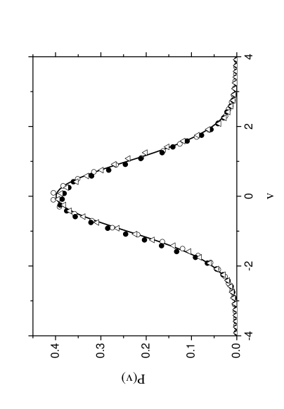
Figure 2 shows the velocity distribution $P(v)$ for graphs with $n=6,10$ and $30$ vertices. The results are averaged over $99$ graphs configurations (approximately $8000$ data points for each configuration). In all the cases presented in Figure 2 the velocity distribution $P(v)$ calculated for quantum graphs is in good agreement with the Gaussian distribution (solid line), as it is expected for quantum chaotic systems. For the other graphs which are not presented in Figure 2 with the number of vertices between $n=6$ and $n=30$ good agreement with the Gaussian distribution is also observed. However, for the graphs with $n=4$ and $n=5$ vertices situation is different (results are not shown). While for the graphs with $n=5$ the agreement with the Gaussian distribution is still quite satisfactory, for the graphs with $n=4$ the velocity distribution is lower than the Gaussian curve for small values of level velocities. This result is not surprising, the graph with $n=4$ is the simplest possible non-trivial fully connected graph one can construct and for some spectral statistics it could be too simple to exhibit behavior that is typical for quantum graphs. But when the number of vertices of a graph increases the agreement with the Gaussian curve improves. For this reason in our further investigation we will concentrate mainly on graphs with $n\geq 6$ vertices.

Figure 3: The level velocity autocorrelation function $c(x)$ for quantum graphs with $n=4$ (crosses), $n=5$ (full diamonds), $n=6$ (open circles), $n=7$ (full squares), $n=10$ (open triangles), $n=20$ (open diamonds) and $n=30$ (full circles) compared to the predictions of RMT for GOE (solid line).

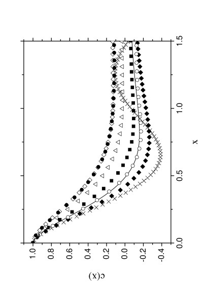
Figure 3 shows the autocorrelation function $c(\mathsf{x})$ calculated for quantum graphs with $n=4,5,6,7,10,20$ and $30$ vertices. In all cases the autocorrelation function $c(\mathsf{x})$ was obtained by averaging over 99 graphs configurations. Numerical results are compared with the results of RMT for GOE (solid line). The numerical simulations of the parameter-dependent autocorrelation function $c(\mathsf{x})$ within RMT for GOE were made using the following Hamiltonian model BruusCorrel

$$H(X)=H_{1}\sin{(X)}+H_{2}\cos{(X)}\mbox{,}$$ (11)

where $H_{1}$, $H_{2}$ are two $500\times 500$ matrices that are members of GOE. In our calculations the parameter $X$ was chosen in 1001 equally spaced points in the interval $[0,\pi/8]$. For each value of the parameter $X$ we ran 99 realizations of $H_{1}$ and $H_{2}$. The eigenvalues obtained from the diagonalization of the Hamiltonian $H(X)$ were unfolded by using the integrated average eigenvalue density for GOE matrices Bohigas et al . The parameter $X$ was unfolded using the formulas (4) and (5).

As it is shown in Figure 3 the autocorrelation function of level velocities $c(\mathsf{x})$ calculated for the graphs with $n=5$ deviates in the downward direction from the RMT predictions for GOE (solid line) for most of the values of the parameter $\mathsf{x}$, while for the graphs with $n\geq 7$ the autocorrelation $c(\mathsf{x})$ deviates in the upward direction from the RMT. The larger graph is, the bigger is deviation from RMT. Only for the graphs with $n=6$ the agreement with RMT is quite good. For the graphs with $n=4$ a strong deviation from RMT is observed for $0.75<\mathsf{x}<1.5$, what is the evidence of a non-universal behavior of the system. It is worth mentioning that the difference between the results obtained for big graphs with $n=20$ and $n=30$ is very small what might suggest that for graphs with $n>30$ the autocorrelation function $c(\mathsf{x})$ converges to the limiting curve which is not given by the RMT predictions for GOE.

The reason of the disagreement of $c(\mathsf{x})$ from the RMT predictions is not exactly known. However, one can assume SchanzScars ; Kaplan01 that it is connected with non-ergodic structures of graphs’ wave functions. In order to check this assumption we calculated the Inverse Participation Ratio (IPR) that is a measure of wave functions localization.

Figure 4: The inverse participation ratio (IPR) calculated for quantum graphs (full circles) compared to the results of random wave hypothesis (solid line). The dotted line shows the minimum values ($I_{min}=1/2B$) of IPR. In the inset we show the distributions $P(\Psi(x))$ of the wave functions $\Psi(x)$ for quantum graphs with $n=4$ (crosses), $n=5$ (full diamonds), $n=6$ (open circles), $n=7$ (full squares), $n=10$ (open triangles), $n=20$ (open diamonds) and $n=30$ (full circles) compared to the Gaussian distribution (solid line). Distributions are presented in double logarithmic scale.

In each bond of a graph a wave function can be written as Kaplan01 :

$$\Psi^{(N)}_{i,j}(x)=a^{(N)}_{i,j}e^{ik_{N}x}+a^{(N)*}_{i,j}e^{-ik_{N}x}.$$ (12)

Then the inverse participation ratio for the N-th energy level can be defined in the following way:

$$I_{N}=\frac{\sum_{2B}|a^{(N)}_{i,j}|^{4}}{\Bigl{[}\sum_{2B}|a^{(N)}_{i,j}|^{2}\Bigr{]}^{2}}.$$ (13)

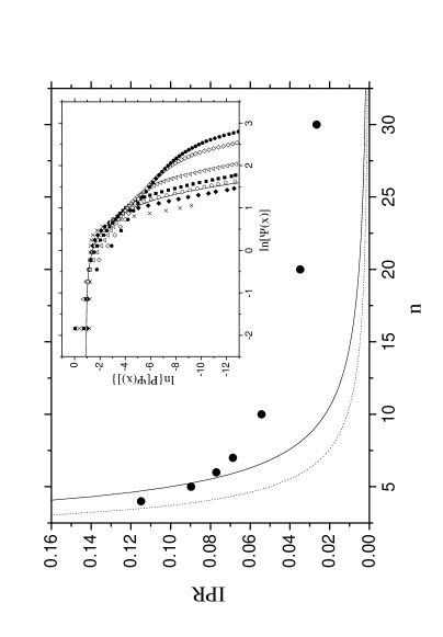
It takes the values between $I_{min}=1/2B$ for states which occupy each directed bond with the same probability and $I_{max}=1$ for a state which is restricted to a single bond only, i.e., the greatest possible degree of localization SchanzScars . Random Wave Hypothesis (RWH) Kaplan01 assumes Gaussian random fluctuations of the complex coefficients $a_{i,j}$. Thus $\langle|a_{i,j}|^{4}\rangle=2$ and $\langle|a_{i,j}|^{2}\rangle=1$. In this case $I_{RWH}\approx 1/B$. In Figure 4 we compare the inverse participation ratio $I_{n}=\langle I_{N}\rangle$ calculated for quantum graphs of different size (circles) with the RWH one (solid line). The averaging in the last formula was performed over the energy levels and over graphs configurations. The dotted line in Figure 4 shows the minimum value ($I_{min}=1/2B$) of IPR. Figure 4 shows that for graphs with $n>5$ the obtained results are bigger then RWH predictions $I_{RWH}$. It means that wave functions of quantum graphs are less ergodic than the ones predicted by Random Wave Model. Furthermore, it is important to noting that the result obtained for the graphs with $n=5$ and $n=6$ vertices are the closest ones to the $I_{RWH}$ predictions.

We also calculated the distributions $P(\Psi(x))$ of the values of the graph wave function $\Psi(x)$ Hlushchuk2001 . The distributions $P(\Psi(x))$ for graphs with $n=4,5,6,10,20$ and $30$, in the double logarithmic scale, are presented in the inset in the Figure 4. The distribution $P(\Psi(x))$ is symmetric, therefore, we considered only positive values of the wave function $\Psi(x)\geq 0$. The inset shows that the distribution $P(\Psi(x))$ obtained for the graphs with $n=6$ (open circles) is the closest one to the Gaussian distribution (solid line) which is the prediction of RMT. Thus, the behavior of $I_{n}$ and $P(\Psi(x))$ for graphs with $n\geq 6$ suggest that the counterintuitive results obtained for the autocorrelation function $c(\mathsf{x})$, where the best agreement with RMT was obtained for the graphs with six vertices, are connected with the localization effects.

The above results suggest that in order to describe numerically the behavior of the autocorrelation function $c(\mathsf{x})$ one can use the concept of coupled M-GOE matrices Alt1998 . A coupled M-GOE matrix with $M\times M$ blocks can be constructed using a random GOE matrix. The values of diagonal blocks elements of the random block matrix are equal to the values of random GOE matrix elements, while the elements of off-diagonal blocks are equal to random GOE matrix elements multiplied by a coupling parameter $0\leq\lambda\leq 1$. By varying $\lambda$ between $1$ and $0$ one can change the coupling between the diagonal blocks of the matrix. In this way a transition between GOE case ($\lambda=1$) and $M$-GOE case ($\lambda=0$) can be achieved. In our numerical study of the parametric level dynamics of coupled M-GOE matrices we applied the Hamiltonian model (11), but instead of $H_{1}$ and $H_{2}$ to be GOE matrices we used two $400\times 400$ coupled M-GOE matrices.

Figure 5: The level velocity autocorrelation function $c(\mathsf{x})$ for quantum graphs with: $n=6$ (open circles), $n=7$ (full squares), $n=10$ (open triangles) and $n=30$ vertices (full circles) compared to the results of RMT (solid line) and coupled M-GOE matrices: $M=3$, $\lambda=0.08$ (dotted line); $M=12$, $\lambda=0.05$ (dash-doted line) and $M=50$, $\lambda=0.03$ (dashed line).

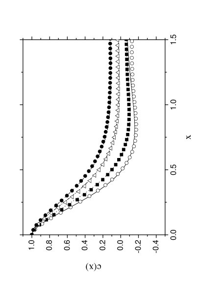
Let us consider the autocorrelation function $c(\mathsf{x})$ for graphs with $n\geq 6$ vertices. Figure 3 shows that the parametric dynamics of graphs with $n=6$ is closely described by RMT for GOE, while large discrepancies observed for graphs with $n>6$ suggests that their properties can be rather described by coupled M-GOE matrices. In order to check this assumption we fitted the values of $\lambda$ and $M$ parameters to describe properly the behavior of the autocorrelation function $c(\mathsf{x})$ for graphs with $n\geq 7$. In Figure 5 the results obtained for quantum graphs with $n=7,10$ and $30$ are compared with corresponding curves for coupled M-GOE matrices with $M=3$, $\lambda=0.08$; $M=12$, $\lambda=0.05$ and $M=50$, $\lambda=0.03$, respectively. In all cases good qualitative agreement between the results for quantum graphs (symbols in Figure 5) and the corresponding ones for coupled M-GOE matrices (lines in Figure 5) is observed.

Figure 6: The integrated nearest neighbor spacing distribution (INNS) for quantum graphs with $n=6$ (open circles), $n=30$ (full circles) and coupled M-GOE matrices with $M=50$ and $\lambda=0.03$ (crosses) compared to the results of RMT for GOE (solid line).

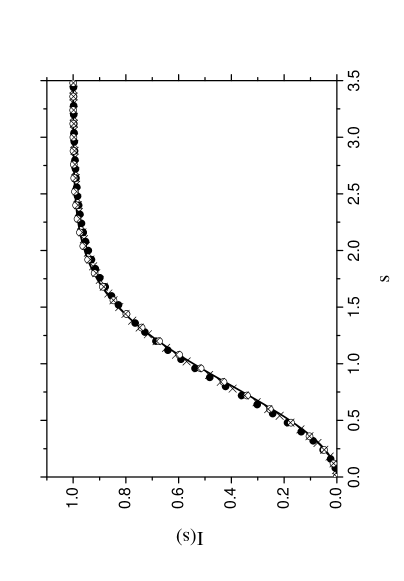
We also calculated the integrated nearest neighbor spacing distribution (INNS) for quantum graphs and coupled M-GOE matrices (see Fig. 6). We found that INNS calculated for graphs with the size between $n=4$ and $n=30$ (in Fig. 6 we show only results for n=6 and n=30) and for coupled M-GOE matrices (in Fig. 6 we show results for matrices with $M=50$ and $\lambda=0.03$) is in good agreement with the prediction of RMT for GOE. This result is very interesting, while INNS and the velocity distribution calculated for quantum graphs are in agreement with RMT for GOE, the autocorrelation function $c(\mathsf{x})$ departures from RMT predictions for GOE and depends on the graph size $n$. It seems that $c(\mathsf{x})$ is much more sensitive to non-universal features of the spectrum and wave functions of the graphs such as eg., scars  SchanzScars ; Kaplan01 than the other considered statistics.

Another important quantity connected with parametric correlations is the velocity autocorrelation function $\tilde{c}(\omega,\mathsf{x})$. From the practical point of view the definition given by the formula (7) is not suitable because it contains delta-function $\delta(x)$. The presence of delta-function means that one should calculate the correlations of level velocities of energy levels separated in energies by exactly the value of $\omega$ from one another. In practice the number of such levels is close to zero. That is why we substituted infinitely narrow delta-function by the weight function $f(x,\delta)$ with the finite width $\delta$, which allows to define an autocorrelation function $\tilde{c}_{\delta}(\omega,\mathsf{x})$ that is more suitable from the practical point of view  SimonsPRBuni

$$\tilde{c}_{\delta}(\omega,\mathsf{x})=\frac{\sum\limits_{ij}\Bigl{<}f\bigl{(}\xi_{i}(\bar{\mathsf{x}}+\mathsf{x})-\xi_{j}(\bar{\mathsf{x}})-\omega,\sqrt{2}\delta\bigr{)}\frac{\partial\xi_{i}(\bar{\mathsf{x}}+\mathsf{x})}{\partial\bar{\mathsf{x}}}\frac{\partial\xi_{j}(\bar{\mathsf{x}})}{\partial\bar{\mathsf{x}}}\Bigr{>}}{\sum\limits_{kl}\bigl{<}f\bigl{(}\xi_{k}(\bar{\mathsf{x}}+\mathsf{x})-\xi_{l}(\bar{\mathsf{x}})-\omega,\sqrt{2}\delta\bigr{)}\bigr{>}}\mbox{.}$$ (14)

In our calculations we used a Gaussian weight function $f(x,\delta)$ SimonsPRBuni

$$f(x,\delta)=\frac{1}{\sqrt{2\pi}\delta}\exp\biggl{(}-\frac{x^{2}}{2\delta^{2}}\biggr{)}\mbox{.}$$ (15)

The autocorrelation function $\tilde{c}_{\delta}(\omega,\mathsf{x})$ defined by the formula (14) allows to calculate correlations of level velocities of energy levels separated mutually by $\omega\pm\delta$.

Figure 7: The velocity autocorrelation function $\tilde{c}(\omega,\mathsf{x})$ for quantum graphs with (a) $n=6$, (b) $n=10$ and (c) $n=30$ compared to the results of RMT for GOE (solid lines) and coupled M-GOE matrices (broken lines). The autocorrelation function $\tilde{c}(\omega,\mathsf{x})$ is calculated for four values of the parameter $\omega$: $\omega=0$ (circles), $\omega=0.1$ (triangles), $\omega=0.25$ (diamonds), and $\omega=1$ (squares).

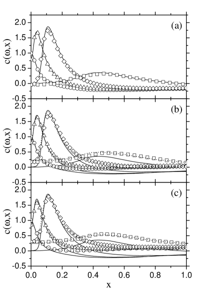
Figures 7a, 7b and 7c show the autocorrelation function of level velocities $\tilde{c}_{\delta}(\omega,\mathsf{x})$ for quantum graphs with $n=6$, $n=10$ and $n=30$ vertices, respectively. Calculations were performed for four values of the parameter $\omega=0,0.1,0.25$ and $1.0$. Similarly to the paper SimonsPRBuni the parameter $\delta$ was chosen to be equal to $0.03$. The numerical curves obtained for quantum graphs are compared with the theoretical ones for GOE in the case of graphs with $n=6$ (Fig. 7a) and for coupled M-GOE matrices for graphs with $n=10$ and $n=30$ (Fig. 7b and Fig. 7c, respectively). In each case the statistical averaging was performed over $99$ graphs configurations.

We found the autocorrelation function $\tilde{c}_{\delta}(\omega,\mathsf{x})$ calculated for graphs with $n=6$ vertices (Fig. 7a) to be in good agreement with the theoretical prediction for GOE (solid lines) for all the values of the $\omega$ parameter. For quantum graphs with $n=10$ and $n=30$ vertices (Fig. 7b and Fig. 7c) the numerical results are in agreement with the ones obtained for coupled M-GOE matrices (broken lines in Fig. 7b and Fig. 7c) for most values of the parameter $\mathsf{x}$. This fact confirms that coupled M-GOE matrices can be successfully used for the description of the parametric dynamics of quantum graphs. However, for some values of $\mathsf{x}$ small deviations from coupled M-GOE matrices results are observed. In Fig. 7a and Fig. 7b the biggest deviation is observed for $\omega=0.25$ in the vicinity of the maximum of the autocorrelation function $\tilde{c}_{\delta}(0.25,\mathsf{x})$.

Let us consider now the level curvatures $\tilde{\kappa}$, the second derivative of the unfolded energies:

$$\tilde{\kappa}_{i}=\frac{\partial^{2}\xi_{i}}{\partial\mathsf{x}^{2}}\mbox{.}$$ (16)

Figure 8: The parametric curvature distribution $P(\kappa)$ for quantum graphs with (a) $n=6$ (open circles), (b) $n=10$ (open triangles) and (c) graphs with $n=30$ vertices (full circles). The numerical results are compared to the results of RMT for GOE (solid line) and for coupled M-GOE matrices (broken line). Results are presented in double logarithmic scale.

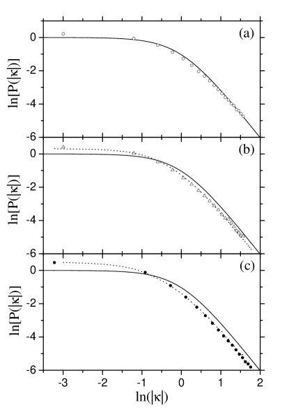
We rescaled the curvatures for quantum graphs using the variance $\sigma_{\mathsf{v}}$:

$$\kappa_{i}=\frac{\tilde{\kappa}_{i}}{\sigma_{\mathsf{v}}}\mbox{.}$$ (17)

The distributions of level curvatures are presented in Fig. 8a, Fig. 8b and Fig. 8c for graphs with $n=6$, $n=10$ and $n=30$, respectively. It is visible that for all of the cases there is no agreement of the obtained results with the GOE prediction (solid line). Only for the graphs with $n=6$ vertices the tail of the distribution can be described correctly by the GOE prediction. For the other graphs the level curvature distributions departure from the GOE one. Therefore, in the case of graphs with $n=10$ and $n=30$ we compare the level curvature distribution with the results obtained for coupled M-GOE matrices (broken line). For the graphs with $n=10$ vertices (Fig. 8b) small deviations from the results for coupled M-GOE matrices are observed only for small values of level curvatures. In the case of graphs with $n=30$ (Fig. 8c) the curvature distribution calculated for coupled M-GOE matrices (broken line) follows the results obtained for the graphs for all of the range of the parameter $\kappa$.

One of the characteristic features of level dynamics of quantum chaotic systems are avoided crossings which are often observed between the neighboring levels when an external parameter $X$ is changed (see Fig. 1 and Fig. 2). We define the avoided crossing distance $C$ as a local minimum of the distance between two neighboring eigenvalues. The distribution of avoided crossings $P(c)$ can be used to distinguish between chaotic systems which belong to different universality classes. The analytical formulas for the distributions of avoided crossings $P(c)$ for GOE and GUE were derived by Zakrzewski and Kuś ZakrzewskiKusAcross . For GOE-systems the distribution of avoided crossings $P(c)$ is the following:

$$P(c)=\frac{2}{\pi}\exp\biggl{(}-\frac{c^{2}}{\pi}\biggr{)}\mbox{.}$$ (18)

To calculate the local minimum $C$ of the avoided crossing distance we used the hyperbolic formula ZakrzewskiAcross :

$$C=\sqrt{d_{2}^{2}-\frac{(d_{3}^{2}-d_{1}^{2})^{2}}{8(d_{3}^{2}+d_{1}^{2}-2d_{2}^{2})}}\mbox{,}$$ (19)

where $d_{i}$, $i=1,2,3$ are three consecutively calculated distances between the adjacent levels. Then avoided crossing distances $C$ obtained in this way are rescaled using the formula:

$$c=\frac{C}{\langle C\rangle}\mbox{,}$$ (20)

where $\langle C\rangle$ is the mean value of avoided crossing distance.

Figure 9: The distribution of avoided crossings $P(c)$ for quantum graphs with $n=6$ (open circles), $n=30$ (full circles) and coupled M-GOE matrices with $M=50$ and $\lambda=0.03$ (crosses) compared to the results of RMT for GOE (solid line).

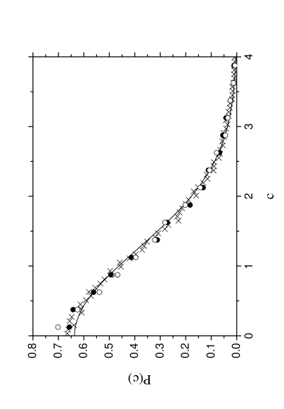
Figure 9 shows the distribution of avoided crossings $P(c)$ for quantum graphs with $n=6$ (open circles), $n=30$ (full circles) and coupled M-GOE matrices with $M=50$ blocks (crosses) compared to the results of RMT for GOE (solid line). The numerical results for graphs were obtained as a result of an averaging over $99$ graph configurations. The distributions of avoided crossings $P(c)$ obtained for graphs show an excess of small values compared to the theoretical prediction for GOE (solid line). However, it is worth noting that in the range of $0.8<c<1.5$ the results obtained for the graphs with $n=6$ vertices are slightly smaller than the RMT prediction for GOE. The results obtained for coupled M-GOE matrices show also an excess of small values comparable to the GOE prediction. However, for $c>0.5$ M-GOE results are close to the ones obtained for the RMT prediction for GOE as well as for the graphs with $n=30$ vertices.

In summary, we investigated numerically eigenvalue dynamics of fully connected irregular quantum graphs with Neumann boundary conditions of different size $n=4-30$. We showed that there are some spectral statistics such as the integrated nearest neighbor spacing distribution, the parametric velocity distribution $P(v)$ and the distribution of avoided crossings $P(c)$ that show no or weak sensitivity to the system size. These statistics show GOE-like behavior. There are also some other statistics, e.g., the second order level velocity autocorrelation functions $c(\mathsf{x})$ and $\tilde{c}(\omega,\mathsf{x})$ and the parametric curvature distribution $P(\kappa)$ that for larger graphs ($n>6$) show deviations from the predictions of RMT for GOE. In all these cases the obtained results are much better described by the model of coupled M-GOE matrices. The agreement of the obtained results with the coupled M-GOE matrices predictions supported by the results of the inverse participation ratio and the distributions $P(\Psi(x))$ suggest the existence of non-ergodic structures of graphs’ wave functions connected with localization which cause the quantum dynamical disintegration of large graphs into the union of weakly interacting smaller graphs.

It is worth pointing out that the agreement of parametric spectral statistics of quantum graphs with the predictions of RMT could be restored by making quantum graphs ”more ergodic”. It could be done by randomizing the boundary conditions at the vertices. For example, one can replace vertex-scattering matrices by random matrices taken from Circular Orthogonal Ensemble (COE) KottosCOE . Our preliminary results, which are not presented here, suggest that in this case parametric spectral statistics show good agreement with RMT predictions for GOE both for smaller and larger graphs. Moreover, this agreement becomes better for larger graphs.

Acknowledgments. We would like to thank Szymon Bauch for valuable comments. This work was supported by the Ministry of Science and Higher Education grant No. N202 099 31/0746. One of the authors, PS, was also supported by the Ministry of Education, Youth and Sports of the Czech Republic within the project LC06002.

References

- (1) N. Savytskyy, A. Kohler, Sz. Bauch, R. Blümel, and L. Sirko, Phys. Rev. E 64, 036211 (2001).
- (2) B.D. Simons and B.L. Altshuler, Phys. Rev. Lett. 70, 4063 (1993).
- (3) B.D. Simons, A. Hashimoto, M. Courtney, D. Kleppner, and B.L. Altshuler, Phys. Rev. Lett. 71, 2899 (1993).
- (4) A. Szaferand B.L. Altshuler, Phys. Rev. Lett 70, 587 (1993).
- (5) B.D. Simons and B.L. Altshuler, Phys. Rev. B 48, 5422 (1993).
- (6) M. Faas, B.D. Simons, X. Zotos, and B.L. Altshuler, Phys. Rev. B 48, 5439 (1993).
- (7) M.V. Berry and J.P. Keating, J. Phys. A 27, 6167 (1994).
- (8) H. Bruus, C.H. Lewenkopf, and E.R. Mucciolo, Phys. Rev. B 53, 9968 (1996).
- (9) Y. Hluszczuk, A. Kohler, Sz. Bauch, L. Sirko, R. Blümel, M. Barth, and H.-J. Stökmann, Phys. Rev. E 61, 366 (2000).
- (10) H. Bruus, C.H. Lewenkopf, and E.R. Mucciolo, Phys. Scr. T69, 13 (1997).
- (11) T. Kottos and U. Smilansky, Ann. Phys. 274, 76 (1999).
- (12) P. Gaspard, S.A. Rice, H.J. Mikeska, and K. Nakasmura, Phys. Rev. A 42, 4015 (1990).
- (13) I.E. Smolyarenko and B.D. Simons, Phys. Rev. E 67, 025202 (2003).
- (14) J. Zakrzewski and M. Kuś, Phys. Rev. Lett. 67, 2749 (1991).
- (15) J. Zakrzewski and D. Delande, Phys. Rev. E 47, 1650 (1993).
- (16) J. Zakrzewski, D. Delande, and M. Kuś, Phys. Rev. E 47, 1665 (1993).
- (17) P. Kunstman, K. Życzkowski, and J. Zakrzewski, Phys. Rev. E 55, 2446 (1997).
- (18) I. Guarneri, K. Życzkowski, J. Zakrzewski, L. Molinari, and G. Casati, Phys. Rev. E 52, 2220 (1995).
- (19) D. Delande and J. Zakrzewski, J. Phys. Soc. Jpn. 63 Suppl. A, 101 (1994).
- (20) J. Zakrzewski, Z. Phys. B 98, 273 (1995).
- (21) G. Berkolaiko, J. P. Keating, and U. Smilansky, Commun. Math. Phys. 273, 137 (2007).
- (22) S. A. Fulling, P. Kuchment, and J. H. Wilson, J. Phys. A 40, 14165 (2007).
- (23) S. Gnutzmann and U. Smilansky, Adv. Phys. 55, 527 (2006).
- (24) P. Pakoński, G. Tanner, and K. Życzkowski, J. Stat. Phys. 111, 1331 (2003).
- (25) P. Exner, M. Helm, and P. Stollmann, Rev. Math. Phys. 19, 923 (2007).
- (26) F. Barra, and P. Gaspard, J. Stat. Phys. 101, 283 (2000).
- (27) T. Kottos and U. Smilansky, Phys. Rev. Lett. 79, 24 (1997).
- (28) O. Hul, P. Šeba and L. Sirko, to be published in Phys. Scr.
- (29) C. Flecia, R. Johnston, and H. Kunz, Europhys. Lett. 3, 497 (1987).
- (30) R. Mitra and S.W. Lee, Analytical Techniques in the Theory of Guided Waves (Macmillan, New York, 1971).
- (31) E.L. Ivchenko and A.A. Kiselev, JETP Lett. 67, 43 (1998).
- (32) J.A. Sanchez-Gil, V. Freilikher, I. Yurkevich, and A.A. Maradudin, Phys. Rev. Lett. 80, 948 (1998).
- (33) Y. Imry, Introduction to Mesoscopic Systems (Oxford University Press, New York, 1996).
- (34) D. Kowal, U. Sivan, O. Entin-Wohlman, and Y. Imry, Phys. Rev. B 42, 9009 (1990).
- (35) O. Hul, Sz. Bauch, P. Pakoński, N. Savytskyy, K. Życzkowski, and L. Sirko, Phys. Rev. E 69, 056205 (2004).
- (36) M. Ławniczak, O. Hul, S. Bauch, P. Šeba, and L. Sirko, Phys. Rev. E 77, 056210 (2008).
- (37) P. Lebœuf, M. Sieber, Phys. Rev. E 60, 3969 (1999).
- (38) O. Bohigas and M.-J. Giannoni, Chaotic motion and Random Matrix Theories, edited by J. S. Dehesa, J. M. G. Gomez, and A. Polls, Lecture Notes in Physics, Vol. 209 (Springer-Verlag, Berlin, 1984), p. 1.
- (39) H. Schanz and T. Kottos, Phys. Rev. Lett. 90, 234101 (2003).
- (40) L. Kaplan, Phys. Rev. E 64, 036225 (2001).
- (41) Y. Hlushchuk, L. Sirko, U. Kuhl, M. Barth, and H.-J. Stöckmann, Phys. Rev. E 63, 046208 (2001).
- (42) H. Alt, C.I. Barbosa, H.-D. Gräf, T. Guhr, H. L. Harney, R. Hofferbert, H. Rehfeld, and A. Richter, Phys. Rev. Lett. 81, 4847 (1998).
- (43) T. Kottos, H. Schanz, Physica E 9, 523 (2001).