The fluctuation-dissipation relation: how does one compare correlation functions and responses?
Abstract
We discuss the well known Einstein and the Kubo Fluctuation Dissipation Relations (FDRs) in the wider framework of a generalized FDR for systems with a stationary probability distribution. A multi-variate linear Langevin model, which includes dynamics with memory, is used as a treatable example to show how the usual relations are recovered only in particular cases. This study brings to the fore the ambiguities of a check of the FDR done without knowing the significant degrees of freedom and their coupling. An analogous scenario emerges in the dynamics of diluted shaken granular media. There, the correlation between position and velocity of particles, due to spatial inhomogeneities, induces violation of usual FDRs. The search for the appropriate correlation function which could restore the FDR, can be more insightful than a definition of “non-equilibrium” or “effective temperatures”.
1 Introduction
The idea of a link between dissipation and fluctuations dates back to Einstein with his work on the Brownian motion [1] and his relation between mobility (which is a non-equilibrium quantity) and diffusion coefficient (which is an equilibrium quantity). Later Onsager [2, 3] with the regression hypothesis and Kubo [4, 5], with linear response theory, investigated in a deep way the issue of the fluctuation-dissipation relation (FDR). In the last decades there has been a renewed interest in this topic, see the contributions of Morris, Evans, Cohen, Gallavotti and Jarzynski [6, 7, 8] to cite just some of the most well known attempts (for a recent review, see [9]).
The FDR theory was originally introduced in the Hamiltonian systems near thermodynamic equilibrium. However it is now clear that a generalized FDR exists, under very general assumptions, for a large class of systems with a “good statistical behaviour”, i.e. with a relaxation to an invariant (smooth) probability distribution. We stress that such a condition is quite common, e.g. in any system with a finite number of degrees of freedom whose evolution rules include some randomness (for instance non-linear Langevin equations). Unfortunately the explicit form of generalized FDR depends on the shape of the invariant probability distribution (which is typically unknown), however this is only a technical difficulty without conceptual consequences [9].
We are not concerned with systems without a stationary probability distribution, e.g. systems showing aging [10, 11] and glassy behaviour [12]. On the contrary, we consider here systems with an invariant probability distribution satisfying the hypothesis for the validity of the generalized FDR mentioned before. For such systems, in our opinion, there is some confusion about what form of FDR has to be expected. When couplings between the chosen observable and other degrees of freedom are ignored, the wrong FDR is expected, i.e. the response function is compared to the wrong correlation: this leads to what is often called a “violation” of FDR.
The structure of the paper is the following: at first, in Section 2, we discuss the different kinds of FDR obtained in the statistical mechanics framework. In Section 3 we analyze a one-dimensional Langevin equation with memory, which can be mapped to a multivariate Langevin equation without memory: this example can be worked out analytically and well illustrates all the main points of our discussion. In section 4 some numerical results on a driven granular gas model are discussed to support our general discussion with physical examples. Section 5 is devoted to concluding remarks.
2 Linear response in statistical mechanics
Let us briefly recall three different kinds of Fluctuation Dissipation Relations (FDR), commonly used in statistical mechanics when a small impulsive perturbation is applied to a stationary system. These three formulae share the feature of relating the system’s linear response to an appropriate two-time correlation computed in the unperturbed system. Anyway these relations have different fields of application and must be adapted with care. For a more pedagogical introduction, we first set the notation, and then we discuss the three FDR versions.
2.1 Linear response functions
We adopt the following notation: denotes the Dirac delta function, and the Kronecker delta, we use the overline for non-stationary averages over many realizations and for averages using the unperturbed stationary probability in phase-space (assuming ergodicity, this is equivalent to a time-average over a long trajectory). Accordingly, we use the shorthand notation
| (1) |
to denote the two-time correlation function between observables and , with the state of the system at time . Let us introduce the matrix of linear response functions, whose element reads
| (2) |
i.e. the mean response of the variable at time to an impulsive perturbation applied to a variable at time . If the dynamics of the system is given, for instance in the form , the mean linear response of the -th degree of freedom to a small perturbation of the -th component of the vector field can be expressed as
| (3) |
The case of an impulsive perturbation at time , , gives back the definition (2).
Let us also consider the historically important case of a Hamiltonian
system at thermal equilibrium: in this case the perturbation is
typically defined on the Hamiltonian, i.e. , with . A linear response function of an observable to an impulsive field at time , determines
the behaviour of for a generic small perturbation :
| (4) |
There are not conceptual differences between the two procedures to perturbe the state (i.e. with a or the introduction of an extra term in the Hamiltonian): we can simply consider and as two variables of the system. For instance, consider the case where is the position of a colloidal particle evolving according to
| (5) |
with independent normalized white noises, i.e. Gaussian processes with and . Here, the effect of a perturbation is equivalent to a and therefore, from a comparison of Eqs. (3) and (4), one has .
2.2 Three different Fluctuation Dissipation Relations
We can now discuss the three forms of FDR we are interested in:
-
1.
the generalized FDR, denoted GFR in the following
(6) where , see below, depends on the invariant distribution density in phase space. This relation is valid (under quite general assumptions, see [13, 14, 15, 16, 17, 9]) in a dynamical system, whose state is completely determined by the phase space coordinate , and whose dynamics induces an invariant measure of phase-space 111more precisely one assumes that is a smooth non-vanishing function. This condition surely holds if some noise is included in the dynamics., and
(7) so that, the correlation reads:
(8) -
2.
the so-called Einstein relation, in the following referred as EFR 222for simplicity we adopt the name “Einstein relation” which, in the literature, has been typically used to denote the time-integral of relation (9), e.g. the formula relating the mobility to the self-diffusion coefficient . ,
(9) The most known example of the above relation is given by a Brownian colloidal particle diffusing in an equilibrium fluid at temperature . Such a system is described by a linear Langevin equation
(10) where is a normalized white noise, i.e. a Gaussian process with and . It is easy to show that after a small impulsive force at time , the velocity perturbation, which at is , decays as . On the other hand, since , where , the EFR (9) holds, with (see [18]). The Green-Kubo relations, relating transport coefficients to the time-integral of unperturbed current-current correlations are the extension of relation (9) to generic transport processes;
-
3.
the classical Kubo relation, hereafter denoted as KFR,
(11) This relation holds - for instance - when a Hamiltonian system, whose statistics is described by the canonical ensemble with temperature , is perturbed by a Hamiltonian variation , which defines the perturbing force and the corresponding conjugate field (see [5, 9]). Relation (11) also holds for Langevin equations with a gradient structure, e.g. Eq. (5). Introducing the quantity 333For this last quantity we use a notation where the second subscript directly refers to the observable conjugate to the perturbed field : even if it is not self-evident, this has the advantage of being coherent with the notation widely used in the literature., from (11) one has
(12) In some literature [19, 20, 21] a deviation from (12) is indicated as a failure of FDR, a mark of being far from equilibrium, and is used to define new “non-equilibrium” temperatures.
As the name suggests, the GFR (iii) includes both EFR (i) and KFR (ii) for some choices of the dynamics or of the stationary distribution [9]. This can be shown for the case and and is easily generalized to any other case, as discussed above:
-
•
GFR EFR: this happens when the invariant distribution in phase space is of the form (being a normalizing constant), then one has and it is immediate to obtain EFR starting from relation GFR;
-
•
GFR KFR: this happens for Hamiltonian systems in the canonical ensemble, or Langevin equations with gradient structure when a small force is applied: in both cases one has , so that the GFR involves the quantity . If the dynamics is given, for instance, by an overdamped Langevin equation of the kind (5), one has that , i.e. and, considering the discussion after Eq. (5), the KFR is immediately derived.
3 Langevin equation with memory
Let us now consider a system that does not necessarily fall neither under the hypothesis of EFR, neither under those of KFR. Our choice here goes to a linear stochastic equation with memory:
| (13) |
where is the mass of the tracer, is the constant of an elastic force, is the friction kernel, is a stochastic force acting as a thermostat.
When there is no memory, i.e. and , the usual Langevin equation is recovered, leading to EFR in the case , Eq. (10), or KFR in the overdamped case, Eq. (5).
For a generic memory kernel, Kubo [5] has also shown that EFR or KFR are recovered, provided that
| (14) |
Here we consider a memory kernel of the kind:
| (15) |
and a noise where and are two independent Gaussian processes with zero means and
| (16) |
so that condition (14) is recovered when (“s” and “f” subscripts stay for “slow” and “fast” respectively). In general, however, . Note also that and have the dimension of a temperature: indeed the model in its overdamped limit has been proposed as an example of system coupled to two different baths acting on different time-scales [19, 20].
3.1 A Markovian equivalent model
The first observation about the system in study is that, because of the memory term, its dynamics after time cannot be deduced by the knowledge of and at time : in fact, the evolution depends on its history, i.e. the dynamics is non-Markovian, and the GFR cannot be directly applied.
However, it is possible to recover Markovianity, at the price of adding additional degrees of freedom. In other words, it is possible (and it will be done in the next section) to recast equation (13) in a linear, multi-dimensional, Langevin equation:
| (17) |
where e are N-dimensional vectors and is a real matrix, in general not symmetric. In addition, now is a Gaussian process, with covariance matrix:
| (18) |
and the real parts of ’s eigenvalues are positive. The stationary probability density is [22]:
| (19) |
where is a symmetric matrix determined by the following relation:
| (20) |
We can now explicitly study the fluctuation and response properties of the system since the dynamics, being now Markovian, satisfies the hypothesis of applicability of GFR. First, we recall the definition of correlation matrix , in the stationary state, which is time-translational invariant. Then, using the equation of motion, it is immediate to verify that , with initial condition given by the covariance matrix between degrees of freedom at equal time: . The corresponding solution is:
| (21) |
Note that, in general and do not commute. It is also straightforward to recover the response function , since the GFR imposes the following equation to hold:
| (22) |
In general this function can be written as:
| (23) |
where are constant matrices, and are the eigenvalues of . The element of the matrix is the response function for the corresponding degrees of freedom. However, at odds with EFR and KFR, this quantity cannot be expressed in terms of the correlation only, since in general all the degrees of freedom are coupled:
| (24) |
which appears as a violation of EFR or KFR, even if GFR is still valid.
In the following, we will explicitly walk through this analysis in two different limit conditions:
-
1.
the free case, when the harmonic force can be neglected;
-
2.
the overdamped case, when inertia can be neglected.
3.2 Dynamics of the free particle
In the limit , and setting without loss of generality, equation (13) becomes
| (25) |
where we have introduced velocity .
Eq. (25) can be mapped to (17) by:
| (26) |
where and are independent normalized white noises, and is an auxiliary variable:
| (27) |
Denoting , , and , a straightforward calculation of covariance matrix gives:
| (28) |
The more general formula for the response as a function of correlations is given by the GFR, Eq. (6):
| (29) |
We can observe two different scenarios: in the case , i.e. , is diagonal with and , condition (14) is restored and, independently by the values of other parameters, a direct proportionality between and is obtained (EFR). This is not the only case for this to happen: e.g. for fixed , one has two possible limits:
| (30) |
respectively for , i.e. , or , i.e. . More in general, when , the coupling term differs from zero and a “violation” of EFR emerges between the coupling of different degrees of freedom.
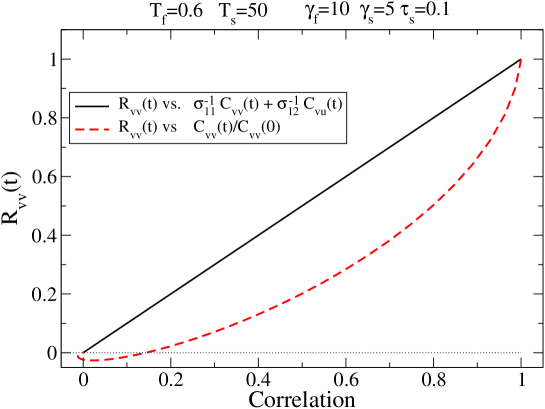
The situation is clarified by Fig. 1, where EFR is violated and the GFR holds: response , when plotted against , shows a non-linear and non-monotonic graph. Anyway a simple linear plot is restored when the response is plotted against the linear combination of correlations indicated by formula (29). In this case it is evident that the “violation” cannot be interpreted by means of any effective temperature: on the contrary it is a consequence of having “missed” the coupling between variables and , which gives an additive contribution to the response of .
It is interesting to note that, even when (i.e. ), is a linear combination of two different exponentials, see Eq. (23), then its derivative is in general not proportional to , i.e. the KFR does not hold. An example of this situation will be discussed in Section 4 and Figure 8.
The above consideration can be easily generalized to the case where several slow thermostats are present: let us suppose that there are thermostats at temperature (the fast one and slow ones) and one at temperature . In this case it is possible to show that the off-diagonal terms in are proportional to .
It is useful to stress the role of Markovianity, which is relevant for a correct prediction of the response. In fact the marginal probability distribution of velocity can be computed straightforward from (25) and has always a Gaussian shape. By that, one could be tempted to conclude, inserting inside GFR, that proportionality between response and correlation holds also if , in contradiction with (28). This conclusion is wrong, as stated at the beginning of this section, because the process is Markovian only if both the variable and the ”hidden” variable are considered.
3.3 Overdamped limit with harmonic potential
When , in the overdamped limit we can neglect the left-hand side term in (13), and the equation, after an integration by parts, reads:
| (31) |
This model has been discussed in the context of driven glassy systems [19, 20].
In order to restore Markovianity, we can map this equation in:
| (32) |
where, as before, and are independent white noises, while the auxiliary variable now reads:
| (33) |
Equation (32) describes the overdamped dynamics of the model depicted in Fig. 2: a first particle at position is coupled to a thermostat with viscosity and temperature , and to the origin by a spring of elastic constant ; a second particle at position is coupled to a thermostat with viscosity and temperature ; the coupling between the two particles is a spring of elastic constant . The first particle, when uncoupled from the second particle, has a characteristic time .

Using non-dimensional parameters and , the covariance matrix reads
| (34) |
where and . As we can see, a diagonal form for the matrix is not recovered, even for , i.e. for this model the EFR never holds.
Let us consider now the KFR, with a force field coupled to the variable . First, we note that, from (22),
| (35) |
(where commutativity between and has been used). Therefore, in general, since , one has
| (36) |
Then, it is easy to see that the condition to have KFR is . Here the matrix reads:
| (37) |
and the condition is equivalent to .
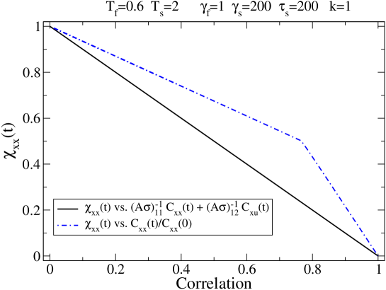
As observed in Fig. 3, in analogy with the previous Fig. 1, the GFR always holds (solid lines), while the KFR is not verified because it ignores the coupling between relevant degrees of freedom. In general the local slope of the parametric curve vs. is given by
| (38) |
which, for the model in Eq. (32), has two different limits:
| (39) | |||||
| (40) |
where
| (41) |
Actually, as observed in [19, 20], when the parametric plot vs. takes the form of a broken line with two slopes: the point where the slope abruptly changes, corresponds to the intermediate plateau of (i.e. when ) and is located at a position on the -axis with : it becomes visible in the plot if (i.e. it is not close to or ). In this case, since , the two slopes are and . This observation has driven a series of real and numerical experiments where the parametric plot vs. (or their Fourier transforms for the frequency-dependent susceptibilities) were measured for some degree of freedom in slowly driven [23] or aging [24, 25] glassy systems, including models for densely packed granular materials [26]. In the next section we discuss this limit and other interesting cases from the point of view of the GFR: this can be useful to understand when the KFR-inspired parametric plot is meaningful and why.
3.4 Phenomenology of the vs. parametric plot
In this section we probe the hypothesis that the relative relevance of the contributions and to the response depends on the time-scale of observation. In particular we consider the time-integrals of these two contributions, such that , see Eq. (36):
| (42) | |||||
| (43) |
The two eigenvalues of the matrix , determining the time-scales of the system and , read:
| (44) |
As suggested by the interpretation given in Fig. 2, the parameters and should act as time-scales when they are separated enough. Indeed, an inspection of formula (44) shows that the inverse of and are proportional to and when they are well separated, i.e. or . However this is a limit case, and more general conditions can be considered.
| case | k | |||||||||
| a | 5 | 0.2 | 20 | 40 | 30 | 20 | 2 | 2/3 | 47.3 | 12.7 |
| b | 2 | 0.6 | 200 | 1 | 200 | 1 | 1 | 1 | 400 | 0.5 |
| c | 2 | 0.6 | 100 | 100 | 2 | 1000 | 0.1 | 50 | 2000 | 1 |
| d | 10 | 2 | 1 | 50 | 10 | 50 | 1 | 0.1 | 51.2 | 9.76 |
Our choices of parameters, always with , are resumed in Table 1: a case (a) where the time-scales are mixed, and three cases (b), (c) and (d) where scales are well separated. In particular, in cases (c) and (d), the position of the intermediate plateau is shifted at one of the extremes of the parametric plot, i.e. only one range of time-scales is visible. Of course we do not intend to exhaust all the possibilities of this rich model, but to offer a few examples which are interesting for the following question: what is the meaning of the usual “incomplete” parametric plot versus , which neglects the contribution of ?
The parametric plots, for the cases of Table 1, are shown in Figure 4. In Figure 5, we present the corresponding contributions and as functions of time. We briefly discuss the four cases:
-
(a)
If the timescales are not separated, the general form of the parametric plot, see Fig. 4a, is a curve. In fact, as shown in Fig. 5a, the cross term is relevant at all the time-scales. The slopes at the extremes of the parametric plot, which can be hard to measure in an experiment, are and . Apart from that, the main information of the parametric plot is to point out the relevance of the coupling of with the “hidden” variable .
-
(b)
In the “glassy” limit , with the constraint , the well known broken line is found, see Fig. 4b, as discussed at the end of the previous section. Figure 5b shows that is negligible during the first transient, up to the first plateau of , while it becomes relevant during the second rise of toward the final plateau.
-
(c)
If , the parametric plot, Fig. 4c, suggests an equilibrium-like behavior (similar to what one expects for ) with an effective temperature which is different from both and . Indeed, this case is quite interesting: the term is of the same order of during all relevant time-scales, but appears to be almost constant. This leads to observe a KFR-like plot with a non-trivial slope. The close similarity between and is due to the high value of the coupling constant .
- (d)
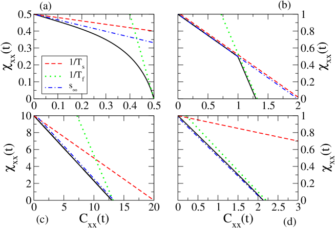
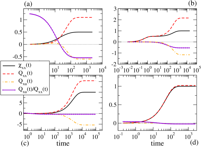
The lesson learnt from this brief study is that the shape of the parametric plot depends upon the timescales and the relative coupling . This is consistent with the fact that the correct formula for the response is always the GFR: . However, the definition of an effective temperature through the relation in general (see case a), does not seem really useful. In particular limits, the behavior of the additional term is such that in a range of time-scales, and therefore the measure of becomes meaningful.
4 Granular gases
In the previous Section we have shown in the analytically tractable
case of linear Langevin equations how the presence of coupling among
different degrees of freedom plays a role in the specific form of
the GFR, which is in general different from the EFR and KFR. Such a
feature is certainly not specific of the considered model: the
non-equilibrium dynamics of a many particles system may present the
same kind of nontrivial correlations among degrees of freedom,
usually due to strong inhomogeneities generated by the lack of
conservation laws valid at equilibrium. In these models the
stationary distribution is not known and the use of the GFR for
response analysis is rather subtle.
In the following we shall
analyze granular gases in the steady state, which offer an
interesting benchmark of this ideas.
4.1 The model
Let us consider a -dimensional model for driven granular gases [27, 28, 29, 30]: identical disks (in ) or rods (in ) of diameter in a volume (in ) or total length (in ) with inelastic hard core interactions characterized by an instantaneous velocity change
| (45) |
where and are the label of the colliding particles, and are the velocity before and after the collision respectively, is the unit vector joining the centers of particles and is the restitution coefficient which is equal to in the elastic case. Each particle is coupled to a “thermal bath”, such that its dynamics (between two successive collisions) obeys
| (46) |
where and are parameters of the “bath” and
are independent normalized white noises. We restrict
ourselves to the dilute or liquid-like regime, excluding more dense
systems where the slowness of relaxation prevents clear measures and
poses doubts about the stationarity of the regime and its ergodicity: in
practice we consider packing fractions (fraction of occupied volume)
in the range . Two important observables of the
system are the mean free time between collisions, , and the
so-called granular temperature .
In this model is possible to recover
two different regimes. When the thermostat is dominant,
i.e. when , grains thermalize, on average, with
the bath before experiencing a collision and the inelastic effects are negligible.
This is an “equilibrium-like” regime, similar to the elastic case , where
the granular gas is spatially homogeneous, the distribution of velocity is Maxwellian and . On the
contrary, when , non-equilibrium effects can emerge such
as deviation from Maxwell-Boltzmann statistics, spatial inhomogeneities and [27, 28, 29, 30].
This “granular regime”, easily reached when packing fraction is increased or inelasticity is reduced,
is characterized by correlations among different particles. This peculiarity is the key
ingredient for a correct response analysis of these systems, as we shall see in the following.
4.2 Failure of the EFR for strong dissipation
An analysis of the FDR for the previous model has been performed in [31, 32] (in ) and [33] (in ), and discussed also in [9]. Similar results are also obtained for other models, such as the inelastic Maxwell model on a lattice driven by a Gaussian thermostat and mean field granular gases [34, 35]. The protocol used in numerical experiments cited above is the following:
-
1.
the gas is prepared in a “thermal” state, with random velocity components extracted from a Gaussian with zero average and given variance, and positions of the particles chosen uniformly random in the box, avoiding overlapping configurations.
-
2.
The system is let evolve until a statistically stationary state is reached, which is set as time : we verify that the total kinetic energy fluctuates around an average value which does not depend on initial conditions.
-
3.
A copy of the system is obtained, identical to the original but for one particle, whose (for instance) velocity component is incremented of a fixed amount .
-
4.
Both systems are let evolve with the unperturbed dynamics. For the random thermostats, the same noise realization is used. The perturbed tracer has velocity , while the unperturbed one has velocity , so that .
-
5.
After a time large enough to have lost memory of the configuration at time , a new copy is done with perturbing a new random particle and the new response is measured. This procedure is repeated until a sufficient collection of data is obtained
-
6.
Finally the autocorrelation function in the original system and the response are measured.
The main result of those studies
can be so summarized: in the dilute limit (where the packing fraction ) or in the elastic limit (), or in the limit of efficient thermostat
(which is usually implied by the dilute limit), the Einstein relation,
Eq. (9), is recovered for the velocity of a tracer particle, i.e. . On the contrary,
when these conditions fails one can observe strong deviations from EFR.
In addiction, there are same remarkable points:
-
•
Non-Gaussian velocity distributions can appear also in the dilute regime, but they seems to have a minor role in the violations of EFR [32].
-
•
The same scenario holds in dimension , where the tracer is sub-diffusive, i.e. where which also implies a non-monotonic with a power-law tail for large [33].
-
•
When a mixture of two different kinds of grains (e.g. with different masses or different restitution coefficients) is considered [36], the two components bear different granular temperatures and this lead to separated FDR in the dilute limit, i.e. a tracer satisfies the EFR with its own temperature, making very difficult to obtain a neutral thermometer based on FDR.
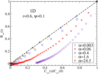
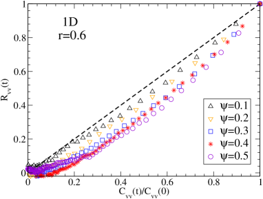
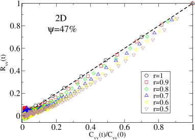
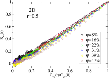
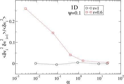
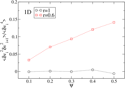
The violation of the EFR is more and more pronounced as the inelasticity increases (lower values of ), the importance of the bath is reduced (lower values of ) or the packing fraction is increased, as shown in Figure 6. In correspondence of such variations of parameters, the correlation between velocities of adjacent particles is also enhanced, a phenomena which is ruled out in equilibrium fluids. This effect can be directly measured in many ways, a possibility is shown in Figure 7. In conclusion, the general lesson is that there is a quite clear correspondence between violations of the EFR and the appearance of correlations among different degrees of freedom.
4.3 A correct prediction of the response
Let us begin with an example explaining how a blind comparison between autocorrelation and response
can be misleading. Clearly the EFR is satisfied in the elastic (“equilibrium”) case,
i.e. , thanks to the fact that,
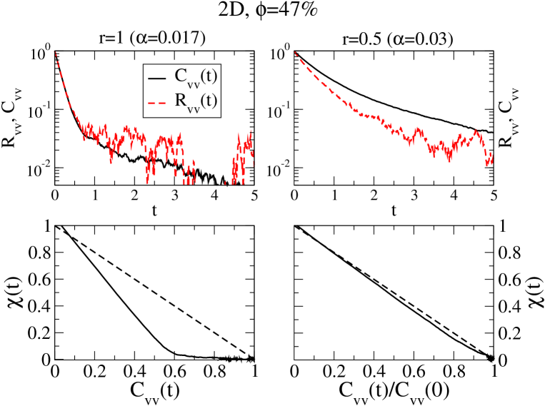
in the invariant measure, there is a very weak coupling between the tracer velocity and other degrees of freedom. However, it is also interesting to note that the shape of is far from being an exponential, also in the elastic (“equilibrium”) case,
because of the presence of two characteristic times and
. This non-exponential shape of leads to a failure of the KFR, Eq. (12), as put in evidence in
the lower left plot of Fig. 8.
It is also instructive to plot the same quantities for a strongly
inelastic case, see right plots of Fig. 8, where an
almost linear relation seems at work.
A first rough explanation is the lower granular temperature which is responsible
for a higher mean free time , implying that and
are slightly closer to each other with respect to the elastic case, making the
similar to a single exponential.
This example show how the only way to have a correct prediction of the response can reside
in the use of the GFR, which is always valid. For a quantitative comparison between correlation functions and response, one needs some hypothesis on the
stationary probability distribution, in particular about the kind of
coupling between different phase-space variables. We report the result
of a simple assumption, partly inspired to an idea of Speck and
Seifert [37], where correlation among variables is mediated by
a fluctuating “hydrodynamic” velocity field , in such a
way that the relevant part of the stationary probability distribution
for the tracer reads, approximately:
| (47) |
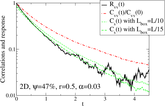
with a local velocity average, defined on a small cell of diameter centered in the particle. This is motivated by the observation that, at high density or inelasticities, spatially structured velocity fluctuations appear in the system for some time, even in the presence of external noise [30, 38]. The generalized FDR following from assumption (47) reads
| (48) |
and is nicely verified in Fig. 9. In other words,
one has a correction to the “naive” expectation , i.e. the extra term originated by the presence of a “hydrodynamic” velocity
field. A recent experiment [39] shows the presence, in a
rather clear way, of a similar extra term (with respect to the KFR)
for a colloidal particle in a toroidal optical trap, in a
non-equilibrium steady state.
We conclude this section underlining
the connections between the results obtained for granular gases and Langevin equations. In general, the
behaviour of the Langevin model and of the granular model show some
differences, for example the case expressed in Figure 4
(case b) has not a counterpart in these models and the “effective
temperature” approach is meaningless, even when times scales are well
separated. However the use of GFR shows how, in both examples, the
response is given by a sum of different contributes, and in some
special limits, the cross correlation term can be neglected and a
comparison between the response and the autocorrelation does make
sense. This happens in the “equilibrium-like” cases of the Langevin
model (cfr. Figure 4, cases c,d) and in the dilute regime
of the granular gas, in which there is no coupling between the velocity
of the tracer and the “hidden variable” embodied by the local
velocity average. On the contrary, when this approximation is not
correct, a response-autocorrelation plot shows strong deviations from
linearity, but can be predicted by taking into account all the
contributes in the computation of the response.
5 Conclusions
In this paper we have reviewed different forms of the fluctuation-dissipation relation for steady states. The most general one is the GFR, Eq. (6), which requires the knowledge of the relevant degrees of freedom and their reciprocal couplings in the system. When this knowledge is not accessible, the study of the response to a perturbation of a certain variable, compared to the correlation of that variable in the unperturbed state, has not a simple meaning, in general.
As an example, we study in detail two limits of a generalized Langevin equation with memory, for a particle which moves in a harmonic potential and is in contact with two thermostats at different temperatures. In the overdamped case, the response-correlation parametric plot may reveal a broken line shape, where the two slopes are given by the inverse temperatures of the baths: a necessary, but not sufficient, condition for this to happen is that time-scales are well separated. In the general case, however, the plot can be more difficult to read, showing intermediate ”effective temperatures”, as well as a more general non-linear shape.
Nevertheless, the problem can be recast as a Markovian dynamics, by means of the introduction of additional degrees of freedoms. The Markovian dynamics has a stationary distribution and satisfies a general relation (GFR) between the response and a specific correlation function, which is related to the stationary measure and takes into account the coupling between degrees of freedom. We show how this coupling is responsible for the ”violation” of the usual FDR.
An interesting case where correlations play a role in the ”violation” of FDR, is the dynamics of a tracer particle in a driven granular gas. Here the response is not proportional, in general, to the unperturbed autocorrelation and an effective temperature does not seem to be informative, even when the time-scales are well separated. Nevertheless a GFR should always be valid, provided an appropriate description of the dynamics is given. Indeed, as already stressed by Onsager and Machlup in their seminal work on fluctuations and irreversible processes [40], a basic ingredient for a “good statistical” description, is Markovianity. We remind their important caveat: how do you know you have taken enough variables, for it to be Markovian? We have seen that, following this suggestion, it is possible to have deeper insight on the so-called “violations of FDR” and in some cases (e.g. in Fig. 9), one can try to guess the correct correlation involved in the dynamics.
Acknowledgments.– We wish to warmly thank L. Leuzzi, U. Marini Bettolo Marconi, F. Ricci-Tersenghi, L. Rondoni and P. Visco for discussions and a critical reading of the manuscript. The work of AP is supported by the “Granular-Chaos” project, funded by the Italian MIUR under the FIRB-IDEAS grant number RBID08Z9JE.
6 References
References
- [1] A Einstein. Investigation on the Theory of the Brownian Motion. Dover, 1956.
- [2] L Onsager. Reciprocal relations in irreversible processes. I. Phys. Rev., 37:405, 1931.
- [3] L Onsager. Reciprocal relations in irreversible processes. II. Phys. Rev., 38:2265, 1931.
- [4] R Kubo. Statistical-mechanical theory of irreversible processes. I. General theory and simple applications to magnetic and conduction problems. J. Phys. Soc. Japan, 12:570, 1957.
- [5] R Kubo. The fluctuation-dissipation theorem. Rep. Prog. Phys., 29:255, 1966.
- [6] D. J. Evans, E. G. D. Cohen, and G. P. Morriss. Probability of second law violations in shearing steady flows. Phys. Rev. Lett., 71:2401, 1993.
- [7] G Gallavotti and E G D Cohen. Dynamical ensembles in stationary states. J. Stat. Phys., 80:931, 1995.
- [8] C Jarzynski. Nonequilibrium equality for free energy differences. Phys. Rev. Lett., 78:2690, 1997.
- [9] U Marini Bettolo Marconi, A Puglisi, L Rondoni, and A Vulpiani. Fluctuation-dissipation: Response theory in statistical physics. Phys. Rep., 461:111, 2008.
- [10] J P Bouchaud, L F Cugliandolo, J Kurchan, and M Mezard. Spin Glasses and Random Fields. World Scientific, 1998.
- [11] E Marinari, G Parisi, F Ricci-Tersenghi, and JJ Ruiz-Lorenzo. Violation of the fluctuation-dissipation theorem in finite-dimensional spin glasses. J. Phys. A., 31:2611, 1998.
- [12] L Leuzzi and Th. M Nieuwenhuizen. Thermodynamics of the Glassy State. Taylor Francis, 2007.
- [13] G S Agarwal. Fluctuation-disipation theorems for systems in non-thermal equilibrium and applications. Z. Physik, 252:25, 1972.
- [14] U Deker and F Haake. Fluctuation-dissipation theorems for classical processes. Phys. Rev. A, 11:2043, 1975.
- [15] P. Hänggi and H. Thomas. Time evolution, correlations and linear response of non-Markov processes. Z. Physik B, 26:85, 1977.
- [16] P. Hänggi and H. Thomas. Stochastic processes: Time-evolution, symmetries and linear response. Phys. Rep., 88:207, 1982.
- [17] M Falcioni, S Isola, and A Vulpiani. Correlation functions and relaxation properties in chaotic dynamics and statistical mechanics. Physics Letters A, 144:341, 1990.
- [18] R Kubo, M Toda, and N Hashitsume. Statistical physics II: Nonequilibrium stastical mechanics. Springer, 1991.
- [19] L F Cugliandolo and J Kurchan. A scenario for the dynamics in the small entropy production limit. J Phys Soc Jpn, 69:247, 2000.
- [20] F Zamponi, F Bonetto, L F Cugliandolo, and J Kurchan. A fluctuation theorem for non-equilibrium relazational systems driven by external forces. J. Stat. Mech., page P09013, 2005.
- [21] A Crisanti and F Ritort. Violation of the fluctuation-dissipation theorem in glassy systems: basic notions and the numerical evidence. J. Phys. A, 36:R181, 2003.
- [22] H Risken. The Fokker-Planck equation: Methods of solution and applications. Springer- Verlag, Berlin, 1989.
- [23] L Berthier and J L Barrat. Shearing a glassy material: Numerical tests of nonequilibrium mode-coupling approaches and experimental proposals. Phys. Rev. Lett., 89:095702, 2002.
- [24] D Hérisson and M Ocio. Fluctuation-dissipation ratio of a spin glass in the aging regime. Phys. Rev. Lett., 88:257202, 2002.
- [25] C Maggi, R di Leonardo, J C Dyre, and G Ruocco. Direct demonstration of fluctuation-dissipation theorem violation in an off-equilibrium colloidal solution. arXiv:0812.0740, 2008.
- [26] M Sellitto. Effective temperature and compactivity of a lattice gas under gravity. Phys. Rev. E, 66:042101, 2002.
- [27] A Puglisi, V Loreto, U M B Marconi, A Petri, and A Vulpiani. Clustering and non-gaussian behavior in granular matter. Phys. Rev. Lett., 81:3848, 1998.
- [28] A Puglisi, V Loreto, U M B Marconi, and A Vulpiani. A kinetic approach to granular gases. Phys. Rev. E, 59:5582, 1999.
- [29] D R M Williams and F C MacKintosh. Driven granular media in one dimension: Correlations and equation of state. Phys. Rev. E, 54:R9, 1996.
- [30] T P C van Noije, M H Ernst, E Trizac, and I Pagonabarraga. Randomly driven granular fluids: Large-scale structure. Phys. Rev. E, 59:4326, 1999.
- [31] A Puglisi, A Baldassarri, and V Loreto. Fluctuation-dissipation relations in driven granular gases. Physical Review E, 66:061305, 2002.
- [32] A Puglisi, A Baldassarri, and A Vulpiani. Violations of the Einstein relation in granular fluids: the role of correlations. J. Stat. Mech., page P08016, 2007.
- [33] D Villamaina, A Puglisi, and A Vulpiani. The fluctuation-dissipation relation in sub-diffusive systems: the case of granular single-file diffusion. J. Stat. Mech., page L10001, 2008.
- [34] A Baldassarri, A Puglisi, and A Vulpiani. Fluctuations and response in granular gases: validity and failure of Einstein relation. In A Co, G L Leal, R H Colby, and A J Giacomin, editors, The XV International Congress on Rheology: The Society of Rheology 80th Annual Meeting, volume 1027 of AIP Conference Proceedings, page 911. AIP, 2008.
- [35] G. Bunin, Y. Shokef, and D. Levine. Frequency-dependent fluctuation–dissipation relations in granular gases. Phys. Rev. E, 77:051301, 2008.
- [36] A Barrat, V Loreto, and A Puglisi. Temperature probes in binary granular gases. Physica A, 334:513, 2004.
- [37] T Speck and U Seifert. Restoring a fluctuation-dissipation theorem in a nonequilibrium steady state. Europhys. Lett., 74:391, 2006.
- [38] E Trizac, I Pagonabarraga, T P C van Noije, and M H Ernst. Randomly driven granular fluids: Collisional statistics and short scale structure. Phys. Rev. E, 65:011303, 2001.
- [39] J R Gomez-Solano, A Petrosyan, S Ciliberto, R Chetrite, and K Gawedzki. Experimental verification of a modified fluctuation-dissipation relation for a micron-sized particle in a non-equilibrium steady state. arXiv:0903.1075, 2009.
- [40] L Onsager and S Machlup. Fluctuations and irreversible processes. Phys. Rev., 91:1505, 1953.