Infrared behavior and spectral function of a Bose superfluid at zero temperature

Abstract

In a Bose superfluid, the coupling between transverse (phase) and longitudinal fluctuations leads to a divergence of the longitudinal correlation function, which is responsible for the occurrence of infrared divergences in the perturbation theory and the breakdown of the Bogoliubov approximation. We report a non-perturbative renormalization-group (NPRG) calculation of the one-particle Green function of an interacting boson system at zero temperature. We find two regimes separated by a characteristic momentum scale $k_{G}$ (“Ginzburg” scale). While the Bogoliubov approximation is valid at large momenta and energies, $|{\bf p}|,|\omega|/c\gg k_{G}$ (with $c$ the velocity of the Bogoliubov sound mode), in the infrared (hydrodynamic) regime $|{\bf p}|,|\omega|/c\ll k_{G}$ the normal and anomalous self-energies exhibit singularities reflecting the divergence of the longitudinal correlation function. In particular, we find that the anomalous self-energy agrees with the Bogoliubov result $\Sigma_{\rm an}({\bf p},\omega)\simeq{\rm const}$ at high-energies and behaves as $\Sigma_{\rm an}({\bf p},\omega)\sim(c^{2}{\bf p}^{2}-\omega^{2})^{(d-3)/2}$ in the infrared regime (with $d$ the space dimension), in agreement with the Nepomnyashchii identity $\Sigma_{\rm an}(0,0)=0$ and the predictions of Popov’s hydrodynamic theory. We argue that the hydrodynamic limit of the one-particle Green function is fully determined by the knowledge of the exponent $3-d$ characterizing the divergence of the longitudinal susceptibility and the Ward identities associated to gauge and Galilean invariances. The infrared singularity of $\Sigma_{\rm an}({\bf p},\omega)$ leads to a continuum of excitations (coexisting with the sound mode) which shows up in the one-particle spectral function.

I Introduction

Following the success of the Bogoliubov theory Bogoliubov (1947) in providing a microscopic explanation of superfluidity, much theoretical work has been devoted to the understanding of the infrared behavior and the calculation of the one-particle Green function of a Bose superfluid not (a). Early attempts to improve the Bogoliubov approximation encountered difficulties due to a singular perturbation theory plagued by infrared divergences Beliaev (1958a, b); Hugenholtz and Pines (1959); Gavoret and Nozières (1964). Although these divergences cancel out in local gauge invariant physical quantities (condensate density, Goldstone mode velocity, etc.), they do have a definite physical origin: they reflect the divergence of the longitudinal susceptibility which is induced by the coupling between transverse (phase) and longitudinal fluctuations. This is a general phenomenon Patasinskij and Pokrovskij (1973) in systems with a continuous broken symmetry as discussed at the end of this section.

Using field-theoretical diagrammatic methods to handle the infrared divergences of the perturbation theory, Nepomnyashchii and Nepomnyashchii (NN) showed that one of the fundamental quantities of a Bose superfluid, the anomalous self-energy $\Sigma_{\rm an}(p)$, vanishes in the limit $p=({\bf p},\omega)\to 0$ in dimension $d\leq 3$, even though the low-energy mode remains phonon-like with a linear spectrum Nepomnyashchii and Nepomnyashchii (1975, 1978); Nepomnyashchii (1983). This exact result shows that the Bogoliubov approximation, where the linear spectrum and the superfluidity rely on a finite value of the anomalous self-energy, breaks down at low energy.

An alternative approach to superfluidity, based on a phase-amplitude representation of the boson field, has been proposed by Popov Popov (1983). This approach is free of infrared singularity, but restricted to the (low-momentum) hydrodynamic regime and therefore does not allow to study the high-momentum or high-frequency regime where the Bogoliubov approximation is expected to be valid. Nevertheless, Popov’s theory Popov and Seredniakov (1979) agrees with the asymptotic low-energy behavior of $\Sigma_{\rm an}(p)$ obtained by NN Nepomnyashchii and Nepomnyashchii (1975, 1978); Nepomnyashchii (1983). Furthermore, the expression of the anomalous self-energy obtained by NN and Popov in the low-energy limit yields a continuum of (one-particle) excitations coexisting with the Bogoliubov sound mode Giorgini et al. (1992), in marked contrast with the Bogoliubov theory where the sound mode is the sole excitation at low energy.

The instability of the Bogoliubov fixed point in dimension $d\leq 3$ towards a different fixed point characterized by the divergence of the longitudinal susceptibility has been confirmed by Castellani et al. Castellani et al. (1997); Pistolesi et al. (2004). Using the Ward identities associated to the local gauge symmetry and a renormalization group approach, these authors obtained the exact infrared behavior of a Bose superfluid at zero temperature. Related results, both at zero Wetterich (2008); Dupuis and Sengupta (2007); Sinner et al. (2009); Dupuis (2009) and finite Andersen99 ; Floerchinger and Wetterich (2008); Floerchinger and Wetterich (2009a, b); Eichler et al. temperature have been obtained by several authors within the framework of the non-perturbative renormalization group.

In this paper, we study a weakly interacting Bose superfluid at zero temperature using the so-called BMW NPRG scheme introduced by Blaizot, Méndez-Galain and Wschebor Blaizot et al. (2006); Benitez09 . Compared to more traditional RG approaches, the NPRG approach presents a number of advantages: i) symmetries are naturally implemented (by a proper Ansatz for the effective action or the two-point vertex (Sec. II)) and Ward identities are naturally satisfied; ii) the NPRG approach is not restricted to the low-energy asymptotic behavior but can deal with all energy scales. In particular, it relates physical quantities at a macroscopic scale to the parameters of the microscopic model; iii) the BMW scheme enables to obtain the full momentum and frequency dependence of the correlation functions Dupuis (2009).

In the NPRG approach, the main quantities of interest are the average effective action $\Gamma_{k}$ (the generating functional of one-particle irreducible vertices) and its second-order functional derivative, the two-point vertex $\Gamma_{k}^{(2)}(p)$, whose inverse gives the one-particle propagator (Sec. II). Fluctuations beyond the Bogoliubov approximation are gradually taken into account as the (running) momentum scale $k$ is lowered from the microscopic scale $\Lambda$ down to zero. In Sec. III, we show that the infrared behavior of the one-particle propagator is entirely determined by the Ward identities associated to the Galilean and local gauge invariances of the microscopic action, and the exponent $3-d$ characterizing the divergence of the longitudinal susceptibility (see the discussion at the end of the Introduction). In Sec. IV we derive the BMW flow equations satisfied by the two-point vertex $\Gamma^{(2)}(p)$ and obtain the analytical solution in the infrared regime. Numerical results are discussed in Sec. V. We find that the Bogoliubov approximation breaks down at a characteristic momentum length $k_{G}$ (“Ginzburg” scale) which, for weak boson-boson interactions, is much smaller than the inverse healing length $k_{h}$ ($k_{h}$ is defined in Appendix A). Although local gauge invariant quantities are not sensitive to $k_{G}$, the effective action $\Gamma_{k}$ is attracted to a fixed point characterized by the divergence of the longitudinal susceptibility when $k\ll k_{G}$. We discuss in detail the frequency and momentum dependence of the two-point vertex $\Gamma^{(2)}_{k}(p)$. While for $|{\bf p}|\gg k_{G}$ or $|\omega|/c\gg k_{G}$ (with $c$ the velocity of the Bogoliubov sound mode), $\Gamma^{(2)}_{k}(p)$ is well described by the Bogoliubov approximation, we reproduce the low-energy asymptotic behavior obtained by NN when $|{\bf p}|,|\omega|/c\ll k_{G}$. In this regime, the longitudinal correlation function becomes singular and its spectral function exhibits a continuum of one-particle excitations in agreement with the predictions of Popov’s hydrodynamic theory. Thus our approach provides a unified picture of superfluidity in interacting boson systems and connects Bogoliubov’s theory to Popov’s hydrodynamic theory. In the conclusion, we comment about a possible extension of our results to strongly interacting or one-dimensional superfluids.

Infrared behavior of interacting bosons

Since the divergence of the longitudinal susceptibility plays a key role in the infrared behavior of interacting boson systems, we first discuss this phenomenon both in classical and quantum systems (for a pedagogical discussion, see also Ref. Weichman (1988)). Let us first consider a $\boldsymbol{\varphi}^{4}$ theory defined by the action

$$S=\frac{1}{2}\int d^{d}r\left\{(\nabla\boldsymbol{\varphi})^{2}+v\boldsymbol{\varphi}^{2}+\frac{\lambda}{4}\bigr{(}\boldsymbol{\varphi}^{2}\bigr{)}^{2}\right\},$$ (1)

where $\boldsymbol{\varphi}({\bf r})$ is a real $N$-component field and $d$ the space dimension. When $v<0$, the mean-field (saddle-point) analysis predicts a non-zero order parameter $\boldsymbol{\varphi}_{0}=\langle\boldsymbol{\varphi}\rangle$. Including Gaussian fluctuations about the saddle-point $\boldsymbol{\varphi}_{0}$, we find a gapped mode and $N-1$ Goldstone modes corresponding to longitudinal ($\delta\boldsymbol{\varphi}\parallel\boldsymbol{\varphi}_{0}$) and transverse ($\delta\boldsymbol{\varphi}\perp\boldsymbol{\varphi}_{0}$) fluctuations, respectively. The correlation functions read

$$\begin{split}G_{\parallel}({\bf p})&=\frac{1}{{\bf p}^{2}+\lambda\boldsymbol{\varphi}_{0}^{2}},\\ G_{\perp}({\bf p})&=\frac{1}{{\bf p}^{2}}.\end{split}$$ (2)

This result, which neglects interactions between longitudinal and transverse fluctuations, is incorrect. In the ordered phase, the amplitude fluctuations of $\boldsymbol{\varphi}$ are gapped and the low-energy effective description is a non-linear $\sigma$ model Zinn_book

$$S[{\bf n}]=\frac{\rho}{2}\int d^{d}r(\boldsymbol{\nabla}{\bf n})^{2},$$ (3)

where ${\bf n}$ is a unit vector (${\bf n}^{2}=1$). To a first approximation, equation (3) can be obtained by setting $\boldsymbol{\varphi}=|\boldsymbol{\varphi}_{0}|{\bf n}$ in (1) (which gives $\rho=\boldsymbol{\varphi}^{2}_{0}$). The non-linear $\sigma$ model is solved by writing ${\bf n}=(\sigma,\boldsymbol{\pi})$ in terms of its longitudinal and transverse components (${\bf n}\cdot\boldsymbol{\varphi}_{0}=\sigma|\boldsymbol{\varphi}_{0}|$ and $\boldsymbol{\pi}\perp\boldsymbol{\varphi}_{0}$). In the low-energy limit, the action (3) describes $N-1$ non-interacting Goldstone modes with propagator $G_{\perp}({\bf p})\sim 1/{\bf p}^{2}$. The longitudinal propagator can be obtained from the constraint ${\bf n}^{2}=\sigma^{2}+\boldsymbol{\pi}^{2}=1$, i.e. $\sigma\simeq 1-\frac{\boldsymbol{\pi}^{2}}{2}$,

$$G_{\parallel}({\bf r})=\langle\sigma({\bf r})\sigma(0)\rangle_{c}\approx\frac{N-1}{2}G^{2}_{\perp}({\bf r})\sim\frac{1}{|{\bf r}|^{2d-4}},$$ (4)

where $\langle\cdots\rangle_{c}$ stands for the connected part of the propagator and $G_{\perp}({\bf r})\sim 1/|{\bf r}|^{d-2}$ denotes the transverse propagator in real space. Equation (4) is obtained by using Wick’s theorem. In Fourier space, we thus obtain

$$G_{\parallel}({\bf p})\sim\frac{1}{|{\bf p}|^{4-d}}\quad({\bf p}\to 0)$$ (5)

for $d<4$ and a logarithmic divergence for $d=4$. Contrary to the predictions of Gaussian theory [Eq. (2)], the longitudinal susceptibility is not finite but diverges for ${\bf p}\to 0$ when $d\leq 4$ Patasinskij and Pokrovskij (1973); Fisher et al. (1973); Anishetty et al. (1999). This divergence is weaker than that of the transverse propagator for all dimensions larger than the lower critical dimension $d_{L}=2$. The appearance of a singularity in the longitudinal channel, driven by transverse fluctuations, is a general phenomenon in systems with a continuous broken symmetry Patasinskij and Pokrovskij (1973). The momentum scale $k_{G}$ below which the Gaussian approximation (2) breaks down is exponentially small for $d=4$ (and $\lambda\to 0$) and of order $\lambda^{1/(4-d)}$ for $d<4$ (see Appendix A.3 for the estimation of $k_{G}$ in a Bose superfluid).

The same conclusion can be drawn from the NPRG analysis of the ordered phase of the linear model (1). The NPRG predicts the coupling constant to scale as $\lambda\sim k^{4-d}$ where $k$ is a running momentum scale Berges et al. (2002). This scaling follows from the flowing of the dimensionless coupling constant $\tilde{\lambda}=\lambda k^{d-4}$ to a finite value $\tilde{\lambda}^{*}$ for $k\to 0$ ($\tilde{\lambda}\sim 1/\ln k$ for $d=4$). The longitudinal propagator then diverges as $G_{\parallel}({\bf p}=0)\sim 1/\lambda\boldsymbol{\varphi}_{0}^{2}\sim 1/k^{4-d}$ and, identifying $k$ with $|{\bf p}|$ to extract the ${\bf p}$ dependence of the propagator, we reproduce (5). Thus, the divergence (5) of the longitudinal susceptibility is a consequence of the fixed point structure of the RG flow in the ordered phase of the linear model (1).

These considerations easily generalize to a quantum model with the Euclidean action

$$S=\frac{1}{2}\int_{0}^{\beta}d\tau\int d^{d}r\biggl{\{}(\nabla\boldsymbol{\varphi})^{2}+c^{-2}({\partial_{\tau}}\boldsymbol{\varphi})^{2}+v\boldsymbol{\varphi}^{2}+\frac{\lambda}{4}\bigr{(}\boldsymbol{\varphi}^{2}\bigr{)}^{2}\biggr{\}},$$ (6)

where $\tau$ is an imaginary time varying between 0 and the inverse temperature $\beta=1/T$, and $c$ the velocity of the Goldstone mode. At zero temperature, we expect the (Euclidean) propagator to behave as

$$\begin{split}G_{\perp}({\bf p},i\omega)&\sim\frac{1}{\omega^{2}+c^{2}{\bf p}^{2}},\\ G_{\parallel}({\bf p},i\omega)&\sim\frac{1}{(\omega^{2}+c^{2}{\bf p}^{2})^{(3-d)/2}},\end{split}\quad({\bf p},\omega\to 0)$$ (7)

where $\omega$ is a Matsubara frequency. (The divergence of $G_{\parallel}$ is logarithmic in three dimensions.) The expression of $G_{\parallel}$ follows from (5) with $|{\bf p}|$ replaced by $(\omega^{2}+c^{2}{\bf p}^{2})^{1/2}$ and $d$ by the effective dimensionality $d+1$ to account for the imaginary time dependence of the field. As in the classical model (1), it can be justified either from an effective low-energy description based on the (quantum) non-linear $\sigma$ model or directly from the linear model (6). After analytical continuation $i\omega\to\omega$, the transverse propagator $G_{\perp}$ exhibits a pole at $\omega=\pm c|{\bf p}|$. On the contrary, $G_{\parallel}$ has no pole-like structure but a branch cut which yields a critical continuum of excitations lying above the Goldstone mode energy $\omega=c|{\bf p}|$. This continuum results from the decay of a normally massive amplitude mode with momentum ${\bf p}$ into a pair of transverse excitations with momenta ${\bf q}$ and ${\bf p}-{\bf q}$ Zwerger (2004).

Interacting bosons are described by a complex field $\psi$ or, equivalently, a two-component real field $(\psi_{1},\psi_{2})$. In the ordered phase, the global U(1) symmetry note2 is broken, giving rise to a gapless (Goldstone) phase mode (the Bogoliubov sound mode). Although the action of non-relativistic bosons differs from the relativistic-type action (6) (see Eq. (13) below), the preceding conclusions regarding the longitudinal propagator still hold in the superfluid phase. The reason is that the argument leading to (7) relies on the existence of a Goldstone mode with linear dispersion $\omega=c|{\bf p}|$ rather than the precise form of the microscopic action. The one-particle propagator in the superfluid phase is usually expressed in terms of a “normal” self-energy, $\Sigma_{\rm n}({\bf p},i\omega)$, and an “anomalous” one, $\Sigma_{\rm an}({\bf p},i\omega)$ Abrikosov et al. (1975); Fetter and Walecka (2003). In Appendix A, we show on general grounds that

$$G_{\parallel}({\bf p},i\omega)\simeq-\frac{1}{2\Sigma_{\rm an}({\bf p},i\omega)}\quad({\bf p},\omega\to 0).$$ (8)

Comparing with (7), we conclude that the anomalous self-energy

$$\Sigma_{\rm an}({\bf p},i\omega)\sim(\omega^{2}+c^{2}{\bf p}^{2})^{(3-d)/2}\quad({\bf p},\omega\to 0)$$ (9)

is singular at low-energy for $d\leq 3$ (the singularity is logarithmic when $d=3$). This singularity, which also shows up in the normal self-energy, is related to the infrared divergences that were encountered early on in the perturbation theory of interacting boson systems Beliaev (1958a, b); Hugenholtz and Pines (1959); Gavoret and Nozières (1964). The exact result $\Sigma_{\rm an}(0,0)=0$ and the asymptotic expression (9) were first obtained by NN from a field-theoretical (diagrammatic) approach Nepomnyashchii and Nepomnyashchii (1975, 1978); Nepomnyashchii (1983). NN’s analysis shows that the infrared behavior markedly differs from the predictions of the Bogoliubov theory ($\Sigma_{\rm an}({\bf p},i\omega)={\rm const}$). One can estimate the momentum “Ginzburg” scale $k_{G}$ below which the Bogoliubov approximation breaks down from perturbation theory Pistolesi et al. (2004); not (b) (see Appendix A),

$$k_{G}\sim\left\{\begin{array}[]{lc}(gmk_{h})^{1/(3-d)}&(d<3),\\ k_{h}\exp\left(-\frac{4\sqrt{2}\pi^{2}}{gmk_{h}}\right)&(d=3).\end{array}\right.$$ (10)

In three dimensions, $k_{G}$ vanishes exponentially when the dimensionless interaction constant $gmk_{h}\to 0$. In two dimensions, the vanishing of $k_{G}$ with $gm$ is only linear.

It was realized by Popov that a phase-density representation of the boson field $\psi=\sqrt{n}e^{i\theta}$ leads to a theory free of infrared divergences Popov (1983); Nepomnyashchii (1983). Popov’s theory is based on an hydrodynamic action $S[n,\theta]$ and is valid below a characteristic momentum $k_{0}$. Since the long-distance physics is governed by the Goldstone (phase) mode, a minimal hydrodynamic description would start from the phase-only action

$$S=\frac{n_{s}}{2m}\int_{0}^{\beta}d\tau\int d^{d}r\left[(\boldsymbol{\nabla}\theta)^{2}+c^{-2}({\partial_{\tau}}\theta)^{2}\right],$$ (11)

where $n_{s}$ is the superfluid density. This action can be obtained from the hydrodynamic action $S[n,\theta]$ by integrating out the density field. It is equivalent to that of the non-linear $\sigma$ model in the $O(N)$ model [Eq. (3)]. Writing $\psi\simeq\sqrt{n}e^{i\theta}$ and expanding with respect to phase fluctuations (with the boson density $n={\rm const}$), one finds

$$\begin{split}G_{\perp}({\bf r}\tau)&=nG_{\theta\theta}({\bf r}\tau),\\ G_{\parallel}({\bf r}\tau)&=\frac{n}{2}G_{\theta\theta}({\bf r}\tau)^{2}\end{split}$$ (12)

for the propagator of the transverse ($\delta\psi=i\sqrt{n}\theta$) and longitudinal ($\delta\psi=-\sqrt{n}\theta^{2}/2$) fluctuations, respectively. $G_{\theta\theta}$ is the phase propagator whose Fourier transform $(m/n_{s})({\bf p}^{2}+\omega^{2}/c^{2})^{-1}$ is read off from (11). In Fourier space, equations (12) coincide with (7). Thus Popov’s approach reproduces the infrared behavior (9) obtained by NN Popov and Seredniakov (1979). The determination of the characteristic momentum $k_{0}$ below which the hydrodynamic approach is valid is non-trivial in the Popov approach as it requires to integrate out all modes with momenta $|{\bf p}|>k_{0}$ to obtain the low-energy hydrodynamic description Popov (1983); Popov and Seredniakov (1979). Interestingly, $k_{0}$ coincides with the Ginzburg scale $k_{G}$ Pistolesi et al. (2004).

II The average effective action

We consider interacting bosons at zero temperature, with the action

$$S=\int dx\left[\psi^{*}(x)\left({\partial_{\tau}}-\mu-\frac{\boldsymbol{\nabla}^{2}}{2m}\right)\psi(x)+\frac{g}{2}|\psi(x)|^{4}\right]$$ (13)

($\hbar=k_{B}=1$ throughout the paper), where $\psi(x)$ is a bosonic (complex) field, $x=({\bf r},\tau)$, and $\int dx=\int_{0}^{\beta}d\tau\int d^{d}r$. $\tau\in[0,\beta]$ is an imaginary time, $\beta\to\infty$ the inverse temperature, and $\mu$ denotes the chemical potential. The interaction is assumed to be local in space and the model is regularized by a momentum cutoff $\Lambda$. We assume the coupling constant $g$ to be weak (dimensionless coupling constant $gm\bar{n}^{1-2/d}\ll 1$, with $\bar{n}$ the mean density) and consider a space dimension $d$ larger than 1. It will often be convenient to write the boson field

$$\psi(x)=\frac{1}{\sqrt{2}}[\psi_{1}(x)+i\psi_{2}(x)]$$ (14)

in terms of two real fields $\psi_{1}$ and $\psi_{2}$.

To define the average effective action Berges et al. (2002), we add to the action (13) a source term $-\int dx(J^{*}\psi+{\rm c.c.})$ and an infrared regulator

$$\Delta S_{k}=\int dxdx^{\prime}\psi^{*}(x)R_{k}(x-x^{\prime})\psi(x^{\prime})$$ (15)

which suppresses fluctuations with momenta and energies below a characteristic scale $k$ but leaves the high-momenta/frequencies modes unaffected. The average effective action

$$\Gamma_{k}[\phi^{*},\phi]={} -\ln Z_{k}[J^{*},J]+\int dx[J^{*}(x)\phi(x)+{\rm c.c.}]$$

$$-\Delta S_{k}[\phi^{*},\phi].$$ (16)

is defined as the Legendre transform of $-\ln Z_{k}[J^{*},J]$, ($Z_{k}[J^{*},J]$ is the partition function) minus the regulator term $\Delta S_{k}[\phi^{*},\phi]$. Here $\phi^{(*)}(x)=\langle\psi^{(*)}(x)\rangle_{J^{*},J}$ is the superfluid order parameter.

The effective action (16) is the generating functional of the one-particle irreducible vertices. The infrared regulator $R_{k}$ is chosen such that for $k=\Lambda$ all fluctuations are frozen. The mean-field theory, where the effective action $\Gamma_{\Lambda}[\phi^{*},\phi]$ reduces to the microscopic action $S[\phi^{*},\phi]$, becomes exact thus reproducing the result of the Bogoliubov approximation [See Eqs. (26) below]. On the other hand for $k=0$, provided that $R_{k=0}$ vanishes, $\Gamma_{k}$ gives the effective action of the original model (13) and allows us to obtain all physical quantities of interest. In practice we take the regulator

$$R_{k}(p)=\frac{Z_{A,k}}{2m}\left({\bf p}^{2}+\frac{\omega^{2}}{c_{0}^{2}}\right)r\left(\frac{{\bf p}^{2}}{k^{2}}+\frac{\omega^{2}}{k^{2}c_{0}^{2}}\right),$$ (17)

where $r(Y)=(e^{Y}-1)^{-1}$ and $p=({\bf p},i\omega)$. The $k$-dependent variable $Z_{A,k}$ is defined below. A natural choice for the velocity $c_{0}$ would be the actual ($k$-dependent) velocity of the Goldstone mode. In the weak coupling limit, however, the Goldstone mode velocity renormalizes only weakly and is well approximated by the $k$-independent value $c_{0}=\sqrt{g\bar{n}/m}$ ($\bar{n}$ is the mean boson density). The regulator (17) differs from previous works where $R_{k}(p)$ was taken frequency independent Wetterich (2008); Dupuis and Sengupta (2007); Sinner et al. (2009); Dupuis (2009). The motivation for the choice (17) will appear clearly when we will discuss the BMW NPRG scheme.

We are primarily interested in the effective potential

$$U(\phi)=\frac{1}{\beta V}\Gamma[\phi]\Bigl{|}_{\phi\,\rm const}$$ (18)

($V$ is the volume of the system) and the two-point vertex

$$\Gamma^{(2)}_{ij}(x,x^{\prime};\phi)=\frac{\delta^{(2)}\Gamma[\phi]}{\delta\phi_{i}(x)\delta\phi_{j}(x^{\prime})}\biggl{|}_{\phi\,\rm const}$$ (19)

computed in a constant, i.e. uniform and time-independent, field. To alleviate the notations, we now drop the $k$ index. We consider $\phi=(\phi_{1},\phi_{2})$ as a two-component real field [see Eq. (14)]. $U$ and $\Gamma^{(2)}_{ij}$ are strongly constrained by the global U(1) invariance of the microscopic action (13) note2 . The effective potential $U(n)$ must be invariant in this transformation and is therefore a function of the condensate density $n=\frac{1}{2}(\phi_{1}^{2}+\phi_{2}^{2})$. The actual ($k$-dependent) condensate density $n_{0}$ is obtained by minimizing the effective potential

$$U^{\prime}(n_{0})=0.$$ (20)

Equation (20) defines the equilibrium state of the system. On the other hand, $\Gamma^{(2)}_{ij}$ must transform as a tensor when the two-dimensional vector $(\phi_{1},\phi_{2})$ is rotated by an arbitrary angle $\alpha$. Since one can form three tensors, $\delta_{i,j}$, $\epsilon_{i,j}$ and $\phi_{i}\phi_{j}$, from the two-dimensional vector $(\phi_{1},\phi_{2})$, the most general form of the two-point vertex is not (c)

$$\Gamma^{(2)}_{ij}(p;\phi)=\delta_{i,j}\Gamma_{A}(p;n)+\phi_{i}\phi_{j}\Gamma_{B}(p;n)+\epsilon_{ij}\Gamma_{C}(p;n)$$ (21)

in Fourier space. $\epsilon_{ij}$ denotes the antisymmetric tensor. In addition, parity and time reversal invariance implies

$$\begin{split}\Gamma^{(2)}_{ij}({\bf p},i\omega;\phi)&=\Gamma^{(2)}_{ij}(-{\bf p},i\omega;\phi),\\ \Gamma^{(2)}_{ij}({\bf p},i\omega;\phi)&=(2\delta_{i,j}-1)\Gamma^{(2)}_{ij}({\bf p},-i\omega;\phi^{*}),\end{split}$$ (22)

where $\phi=(\phi_{1},\phi_{2})$ and $\phi^{*}=(\phi_{1},-\phi_{2})$. From (21) and (22) we deduce

$$\begin{split}\Gamma_{A}(p;n)&=\Gamma_{A}(-p;n)=\Gamma_{A}({\bf p},-i\omega;n),\\ \Gamma_{B}(p;n)&=\Gamma_{B}(-p;n)=\Gamma_{B}({\bf p},-i\omega;n),\\ \Gamma_{C}(p;n)&=-\Gamma_{C}(-p;n)=-\Gamma_{C}({\bf p},-i\omega;n).\end{split}$$ (23)

For $p=0$, we can relate the two-point vertex to the derivatives of the effective potential,

$$\Gamma^{(2)}_{ij}(p=0;\phi)=\frac{\partial^{2}U(n)}{\partial\phi_{i}\partial\phi_{j}}=\delta_{i,j}U^{\prime}(n)+\phi_{i}\phi_{j}U^{\prime\prime}(n),$$ (24)

so that

$$\begin{split}\Gamma_{A}(p=0;n)&=U^{\prime}(n),\\ \Gamma_{B}(p=0;n)&=U^{\prime\prime}(n),\\ \Gamma_{C}(p=0;n)&=0.\end{split}$$ (25)

For $k=\Lambda$, one has $\Gamma_{k}[\phi]=S[\phi]$ and therefore

$$\begin{split}U_{k=\Lambda}(n)&=-\mu n+\frac{g}{2}n^{2}=-\frac{1}{2}gn_{0}^{2}+\frac{g}{2}(n-n_{0})^{2},\\ \Gamma_{A,k=\Lambda}(p;n)&=\epsilon_{\bf p}+g(n-n_{0}),\\ \Gamma_{B,k=\Lambda}(p;n)&=g,\\ \Gamma_{C,k=\Lambda}(p;n)&=\omega,\end{split}$$ (26)

where $n_{0}\equiv n_{0,k=\Lambda}=\mu/g$.

We can also relate the two-point vertex to the normal and anomalous self-energies that are usually introduced in the theory of superfluidity Abrikosov et al. (1975); Fetter and Walecka (2003),

$$\begin{split}\Sigma_{\rm n}(p)={}&i\omega+\mu-\epsilon_{\bf p}+\bar{\Gamma}_{A}(p)+n_{0}\bar{\Gamma}_{B}(p)-i\bar{\Gamma}_{C}(p),\\ \Sigma_{\rm an}(p)={}&n_{0}\bar{\Gamma}_{B}(p)\end{split}$$ (27)

(see Appendix A), where $\bar{\Gamma}_{\alpha}(p)=\Gamma_{\alpha}(p;n_{0})$ ($\alpha=A,B,C$) denotes the two-point vertex in the equilibrium state ($n=n_{0}$).

In the equilibrium state ($n=n_{0}$), the transverse part not (c) $\bar{\Gamma}_{A}(p=0)=U^{\prime}(n_{0})$ of the two-point vertex vanishes. This result is a consequence of the invariance of the effective action $\Gamma[\phi]$ in a global U(1) transformation and reflects the existence of a (gapless) Goldstone mode. When expressed in terms of the normal and anomalous self-energies (27) (with the condition $\bar{\Gamma}_{C}(p=0)=0$), it reproduces the Hugenholtz-Pines theorem Hugenholtz and Pines (1959) (87).

III Derivative expansion and infrared behavior

On the basis of the arguments given in the Introduction, we expect the anomalous self-energy

$$\bar{\Gamma}_{k=0,B}(p)\sim(\omega^{2}+c^{2}{\bf p}^{2})^{(3-d)/2}\quad({\bf p},\omega\to 0)$$ (28)

to be singular in the low-energy limit (see Eqs. (9) and (27)). From (28), we infer

$$\bar{\Gamma}_{B}(p=0)=U^{\prime\prime}(n_{0})\sim k^{3-d}\quad(k\to 0).$$ (29)

Equation (29) will be obtained in Sec. IV from the NPRG equations. In this section, we show that it is sufficient, when combined with Ward identities associated to Galilean and gauge invariances Gavoret and Nozières (1964); Huang and Klein (1964); Pistolesi et al. (2004), to obtain the infrared behavior of the propagators.

The infrared regulator (17) ensures that the vertices are regular functions of $p$ for $|{\bf p}|\ll k$ and $|\omega|/c\ll k$, even when they become singular functions of $({\bf p},i\omega)$ at $k=0$ ($c\simeq c_{0}$ is the velocity of the Goldstone mode defined below) not (d). In the low-energy limit $|{\bf p}|,|\omega|/c\ll k$, we can then use the derivative expansion

$$\begin{split}\bar{\Gamma}_{A}(p)&\simeq Z_{A}\epsilon_{\bf p}+V_{A}\omega^{2},\\ \bar{\Gamma}_{B}(p)&\simeq U^{\prime\prime}(n_{0})=\lambda,\\ \bar{\Gamma}_{C}(p)&\simeq Z_{C}\omega,\end{split}$$ (30)

consistent with $\bar{\Gamma}_{A}(p=0)=0$ and the symmetry properties (23). To obtain (30) we have expanded $\bar{\Gamma}_{B}(p)$ only to leading order, dropping the next-order term $Z_{B}\epsilon_{\bf p}+V_{B}\omega^{2}$. Because of the singularity (28), the coefficients $Z_{B}$ and $V_{B}$ would diverge for $k\to 0$ contrary to $Z_{A}$, $Z_{C}$ and $V_{A}$ that reach finite values. The justification for neglecting the $p$ dependence of the vertex $\bar{\Gamma}_{B}$ comes from the fact that for $d>1$, $\lambda={\cal O}(k^{3-d})$ is a very large energy scale with respect to $\bar{\Gamma}_{A},\bar{\Gamma}^{2}_{C}$ for typical momentum and frequency $|{\bf p}|,|\omega|/c\sim k$. The $p$ dependence of $\bar{\Gamma}_{B}(p)$ does not change the leading behavior of $\bar{\Gamma}_{B}(p)\sim{\cal O}(k^{3-d})$ which essentially acts as a large mass term in the propagators.

III.1 Goldstone mode velocity and superfluid density

The excitation spectrum can be obtained from the zeros of the determinant of the $2\times 2$ matrix $\bar{\Gamma}^{(2)}_{ij}(p)$ (after analytical continuation $i\omega\to\omega+i0^{+}$),

$${\rm det}\,\bar{\Gamma}^{(2)}(p) =\bar{\Gamma}_{A}(p)[\bar{\Gamma}_{A}(p)+2n_{0}\bar{\Gamma}_{B}(p)]+\bar{\Gamma}^{2}_{C}(p)$$

$$\simeq 2n_{0}\bar{\Gamma}_{B}(0)\bar{\Gamma}_{A}(p)+\bar{\Gamma}^{2}_{C}(p)$$

$$\simeq 2n_{0}\lambda(Z_{A}\epsilon_{\bf p}+V_{A}\omega^{2})+(Z_{C}\omega)^{2},$$ (31)

where the approximate equality is obtained using $\bar{\Gamma}_{B}(p)\sim k^{3-d}$, $\bar{\Gamma}_{A}(p),\bar{\Gamma}^{2}_{C}(p)\sim{\bf p}^{2},\omega^{2}$ and $|{\bf p}|,|\omega|/c\ll k$. Equation (31) agrees with the existence of a Goldstone mode (the Bogoliubov sound mode) with velocity

$$c=\left(\frac{Z_{A}/(2m)}{V_{A}+Z_{C}^{2}/(2\lambda n_{0})}\right)^{1/2}.$$ (32)

The low-energy expansion (30) can also be used to define the superfluid density $n_{s}$. Suppose the phase $\theta({\bf r})$ of the order parameter $\phi({\bf r})=\sqrt{2n_{0}}(\cos\theta({\bf r}),\sin\theta({\bf r}))$ varies slowly in space. To lowest order in $\boldsymbol{\nabla}\theta$, the average effective action will increase by

$$\delta\Gamma =\frac{1}{2}\sum_{p}\bar{\Gamma}^{(2)}_{A}(p)\phi_{2}(-p)\phi_{2}(p)$$

$$=n_{0}\sum_{\bf p}\bar{\Gamma}^{(2)}_{A}({\bf p},\omega=0)\theta(-{\bf p})\theta({\bf p})$$

$$=\frac{Z_{A}n_{0}}{2m}\beta\int d^{d}r(\boldsymbol{\nabla}\theta)^{2}.$$ (33)

Identifying the phase stiffness with the superfluid density Chaikin and Lubensky (1995), we obtain

$$n_{s}=Z_{A}n_{0}.$$ (34)

III.2 Symmetries and thermodynamic relations

The two-point vertex satisfies the following relations,

$$\begin{split}\frac{\partial}{\partial{\bf p}^{2}}\bar{\Gamma}_{A}(p)\Bigl{|}_{p=0}&=\frac{\bar{n}}{2mn_{0}},\\ \frac{\partial}{\partial\omega^{2}}\bar{\Gamma}_{A}(p)\Bigl{|}_{p=0}&=-\frac{1}{2n_{0}}\frac{\partial^{2}U}{\partial\mu^{2}}\biggl{|}_{n_{0}},\\ \frac{\partial}{\partial\omega}\bar{\Gamma}_{C}(p)\Bigl{|}_{p=0}&=-\frac{\partial^{2}U}{\partial n\partial\mu}\biggl{|}_{n_{0}},\end{split}$$ (35)

which follow from Ward identities associated with Galilean (for the first one) and local gauge (for the last two) invariance (see Appendix B). Here we consider the effective potential $U(n,\mu)$ as a function of the two independent variables $n$ and $\mu$. The condensate density $n_{0}=n_{0}(\mu)$ is then defined by

$$\frac{\partial U}{\partial n}\biggl{|}_{n_{0}}=0,$$ (36)

while the mean boson density is obtained from

$$\bar{n} =-\frac{d}{d\mu}U(n_{0},\mu)$$

$$=-\frac{\partial U}{\partial\mu}\biggl{|}_{n_{0}}-\frac{\partial U}{\partial n}\biggl{|}_{n_{0}}\frac{dn_{0}}{d\mu}=-\frac{\partial U}{\partial\mu}\biggl{|}_{n_{0}},$$ (37)

where $d/d\mu$ is a total derivative. Equation (36) being valid for any $\mu$, one deduces

$$\frac{d}{d\mu}\frac{\partial U}{\partial n}\biggl{|}_{n_{0}}=\frac{\partial^{2}U}{\partial n\partial\mu}\biggl{|}_{n_{0}}+\frac{\partial^{2}U}{\partial n^{2}}\biggl{|}_{n_{0}}\frac{dn_{0}}{d\mu}=0.$$ (38)

From (35) and (38), one deduces

$$\begin{split}n_{s}&=Z_{A}n_{0}=\bar{n},\\ V_{A}&=-\frac{1}{2n_{0}}\frac{\partial^{2}U}{\partial\mu^{2}}\biggl{|}_{n_{0}},\\ Z_{C}&=-\frac{\partial^{2}U}{\partial n\partial\mu}\biggl{|}_{n_{0}}=\lambda\frac{dn_{0}}{d\mu}.\end{split}$$ (39)

The first of these equations states that in a Galilean invariant superfluid at zero temperature, the superfluid density is given by the full density of the fluid Gavoret and Nozières (1964). The velocity (32) can be rewritten as

$$c^{2}=\frac{\bar{n}}{m}\frac{1}{-\frac{\partial^{2}U}{\partial\mu^{2}}\Bigl{|}_{n_{0}}+\frac{\partial^{2}U}{\partial n^{2}}\Bigl{|}_{n_{0}}\bigl{(}\frac{dn_{0}}{d\mu}\bigr{)}^{2}}.$$ (40)

Comparing with

$$\frac{d\bar{n}}{d\mu}=-\frac{\partial^{2}U}{\partial\mu^{2}}\biggl{|}_{n_{0}}+\frac{\partial^{2}U}{\partial n^{2}}\biggl{|}_{n_{0}}\left(\frac{dn_{0}}{d\mu}\right)^{2},$$ (41)

we deduce that the Goldstone mode velocity

$$c=\left(\frac{\bar{n}}{m(d\bar{n}/d\mu)}\right)^{1/2}$$ (42)

is equal to the macroscopic sound velocity Gavoret and Nozières (1964).

Since thermodynamic quantities, including the condensate “compressibility” $dn_{0}/d\mu$ should be finite, we deduce from (39) that $Z_{C}\sim k^{3-d}$ vanishes in the infrared limit, and

$$\lim_{k\to 0}c=\lim_{k\to 0}\left(\frac{Z_{A}}{2mV_{A}}\right)^{1/2}.$$ (43)

Both $Z_{A}=\bar{n}/n_{0}$ and the macroscopic sound velocity $c$ being finite, $V_{A}$ (which vanishes in the Bogoliubov approximation) takes a non-zero value. In the infrared limit, the $\omega^{2}$ term of $\bar{\Gamma}_{A}(p)$ is therefore crucial to maintain a linear spectrum and superfluidity. As discussed in more detail in Sec. IV.3, the expression (43) is a manifestation of the relativistic invariance of the effective action which emerges in the low-energy limit.

III.3 One-particle propagator

We are now in a position to deduce the infrared limit of the one-particle propagator $G_{ij}$. For symmetry reasons (see Sec. II),

$$G_{ij}(p;\phi)={} \frac{\phi_{i}\phi_{j}}{2n}G_{\rm ll}(p;n)+\left(\delta_{ij}-\frac{\phi_{i}\phi_{j}}{2n}\right)G_{\rm tt}(p;n)$$

$$+\epsilon_{ij}G_{\rm lt}(p;n)$$ (44)

for a constant field $\phi$, where

$$\begin{split}G_{\rm ll}(p;n)&=-\frac{\Gamma_{A}(p;n)}{D(p;n)},\\ G_{\rm tt}(p;n)&=-\frac{\Gamma_{A}(p;n)+2n\Gamma_{B}(p;n)}{D(p;n)},\\ G_{\rm lt}(p;n)&=\frac{\Gamma_{C}(p;n)}{D(p;n)},\end{split}$$ (45)

and $D=\Gamma_{A}^{2}+2n\Gamma_{B}\Gamma_{A}+\Gamma_{C}^{2}$. Equations (45) follow from the matrix relation $G^{-1}=-\Gamma^{(2)}$. Using $\lambda,Z_{C}\sim k^{3-d}\gg k^{2}$, we then find

$$D(p)\simeq 2n_{0}\lambda V_{A}(\omega^{2}+c^{2}{\bf p}^{2})$$ (46)

and

$$\begin{split}\bar{G}_{\rm ll}(p)&=-\frac{1}{2n_{0}\lambda},\\ \bar{G}_{\rm tt}(p)&=-\frac{1}{V_{A}}\frac{1}{\omega^{2}+(c{\bf p})^{2}}=-\frac{2n_{0}mc^{2}}{\bar{n}}\frac{1}{\omega^{2}+(c{\bf p})^{2}},\\ \bar{G}_{\rm lt}(p)&=\frac{Z_{C}}{2n_{0}\lambda V_{A}}\frac{\omega}{\omega^{2}+(c{\bf p})^{2}}=\frac{mc^{2}}{\bar{n}}\frac{dn_{0}}{d\mu}\frac{\omega}{\omega^{2}+(c{\bf p})^{2}}.\end{split}$$ (47)

The propagators $\bar{G}_{\rm tt}$ and $\bar{G}_{\rm lt}$ have well defined limits when $k\to 0$, while the longitudinal propagator $\bar{G}_{\rm ll}\sim 1/k^{(3-d)}$ diverges in agreement with the general discussion of the Introduction. Stricto sensu, equations (47) hold in the limit $|{\bf p}|,|\omega|/c\ll k$. We can nevertheless obtain the propagators at $k=0$ and finite $({\bf p},i\omega)$ by stopping the flow at $k\sim\sqrt{{\bf p}^{2}+\omega^{2}/c^{2}}$ (see the discussion in Sec. IV.3). Since the local gauge invariant (thermodynamic) quantities are not expected to flow in the infrared limit (Sec. V), this procedure amounts to replacing $n_{0}$, $\bar{n}$, $c$ and $dn_{0}/d\mu$ by their $k=0$ values. As for the longitudinal correlation function, we reproduce the expected infrared singularity

$$\bar{G}_{\rm ll}(p)=-\frac{1}{2n_{0}C[\omega^{2}+(c{\bf p})^{2}]^{(3-d)/2}}.$$ (48)

The constant $C$ can be estimated by comparing (48) with the result of Popov’s hydrodynamic theory Giorgini et al. (1992),

$$C\simeq\left(\frac{2\bar{n}}{mcn_{0}}\right)^{2}.$$ (49)

From these results, we deduce the infrared behavior of the normal and anomalous propagators

$$\begin{split}G_{\rm n}(p)={}&-\langle\psi(p)\psi^{*}(p)\rangle\\ ={}&-\frac{n_{0}mc^{2}}{\bar{n}}\frac{1}{\omega^{2}+(c{\bf p})^{2}}\\ &-\frac{mc^{2}}{\bar{n}}\frac{dn_{0}}{d\mu}\frac{i\omega}{\omega^{2}+(c{\bf p})^{2}}+\frac{1}{2}\bar{G}_{\rm ll}(p),\\ G_{\rm an}(p)={}&-\langle\psi(p)\psi(-p)\rangle\\ ={}&\frac{n_{0}mc^{2}}{\bar{n}}\frac{1}{\omega^{2}+(c{\bf p})^{2}}+\frac{1}{2}\bar{G}_{\rm ll}(p).\end{split}$$ (50)

The leading order terms in (50) agree with the results of Gavoret and Nozières Gavoret and Nozières (1964). The contribution of the diverging longitudinal correlation function was first identified by NN, and later in Refs. Weichman (1988); Giorgini et al. (1992); Castellani et al. (1997); Pistolesi et al. (2004).

IV RG equations

To compute approximately the effective potential $U$ and the one-particle propagator, we follow the BMW NPRG scheme proposed in Refs. Blaizot et al. (2006); Benitez et al. (2008); Benitez09 with a truncation in fields to lowest non-trivial order Guerra et al. (2007).

IV.1 BMW equations

The dependence of the effective action on $k$ is given by Wetterich’s equation Wetterich (1993)

$$\partial_{t}\Gamma[\phi]=\frac{1}{2}{\rm Tr}\left\{\dot{R}\bigl{(}\Gamma^{(2)}[\phi]+R\bigr{)}^{-1}\right\},$$ (51)

where $t=\ln(k/\Lambda)$ and $\dot{R}=\partial_{t}R$. In Fourier space, the trace involves a sum over frequencies and momenta as well as a trace over the two components of the field $\phi=(\phi_{1},\phi_{2})$.

The flow equation for the effective potential $U(n)=(\beta V)^{-1}\Gamma[\phi]$ (with $\phi=(\sqrt{2n},0)$ is directly derived from (51),

$$\partial_{t}U(n)=-\frac{1}{2}\int_{p}\dot{R}(p)[G_{\rm ll}(p;n)+G_{\rm tt}(p;n)],$$ (52)

where

$$\int_{p}=\int_{\bf p}\int_{\omega}=\int\frac{d^{d}p}{(2\pi)^{d}}\int_{-\infty}^{\infty}\frac{d\omega}{2\pi}.$$ (53)

The flow equation of the condensate density is then deduced from

$$\partial_{t}U^{\prime}(n_{0})=\partial_{t}U^{\prime}|_{n_{0}}+U^{\prime\prime}(n_{0})\partial_{t}n_{0}=0,$$ (54)

while that of $\lambda=U^{\prime\prime}(n_{0})$ is obtained from

$$\partial_{t}\lambda=\partial_{t}U^{\prime\prime}|_{n_{0}}+U^{\prime\prime\prime}(n_{0})\partial_{t}n_{0}.$$ (55)

Note that the propagator $G$ in (52) and below is defined as the inverse of $-(\Gamma^{(2)}+R)$.

Equation (51) leads to a flow equation for the two-point vertex $\Gamma^{(2)}$ which involves the three-point and four-point vertices,

$$\partial_{t}\Gamma^{(2)}_{ij}(p;\phi)=\\ -\frac{1}{2}\sum_{q,i_{1},i_{2}}\tilde{\partial}_{t}G_{i_{1}i_{2}}(q;\phi)\Gamma^{(4)}_{iji_{2}i_{1}}(p,-p,q,-q;\phi)\\ -\frac{1}{2}\sum_{q,i_{1}\cdots i_{4}}\Bigl{\{}\Gamma^{(3)}_{ii_{2}i_{3}}(p,q,-p-q;\phi)\Gamma^{(3)}_{ji_{4}i_{1}}(-p,p+q,-q;\phi)\\ \times[\tilde{\partial}_{t}G_{i_{1}i_{2}}(q;\phi)]G_{i_{3}i_{4}}(p+q;\phi)+(p\leftrightarrow-p,i\leftrightarrow j)\Bigr{\}},$$ (56)

where the operator $\tilde{\partial}_{t}=(\partial R/\partial t)\partial_{R}$ acts only on the $t$ dependence of the regulator $R$. The field $\phi$ is assumed to be uniform and time independent.

The BMW approximation is based on the following two observations Blaizot et al. (2006): i) Since the function $\tilde{\partial}_{t}G_{ij}(q;\phi)$ is proportional to $\partial_{t}R(q)$, the integral over the loop variable $q=({\bf q},i\omega)$ in (56) is dominated by values of $|{\bf q}|$ and $|\omega|/c$ smaller than $k$. (Note that this argument requires a regulator $R(q)$ that acts both on momentum and frequency.). ii) As they are regulated in the infrared, the vertices $\Gamma^{(n)}$ are smooth functions of momenta and frequencies not (d). These two properties allow one to make an expansion in power of ${\bf q}^{2}/k^{2}$ and $\omega^{2}/(ck)^{2}$, independently of the value of the external variable $p=({\bf p},i\omega_{\nu})$. To leading order, one simply sets $q=0$ in the three- and four-point vertices. We can then obtain a close equation for $\Gamma^{(2)}_{ij}(p;\phi)$ by noting that Blaizot et al. (2006)

$$\begin{split}\Gamma^{(3)}_{ijl}(p,-p,0;\phi)&=\frac{1}{\sqrt{\beta V}}\frac{\partial}{\partial\phi_{l}}\Gamma^{(2)}_{ij}(p;\phi),\\ \Gamma^{(4)}_{ijlm}(p,-p,0,0;\phi)&=\frac{1}{\beta V}\frac{\partial^{2}}{\partial\phi_{l}\partial\phi_{m}}\Gamma^{(2)}_{ij}(p;\phi).\end{split}$$ (57)

The flow equation for $\Gamma_{\alpha}(p;n)$ is given in Appendix C [Eqs (113-115)].

IV.2 Truncated flow equations

We simplify the BMW equations by considering two additional approximations. First we define the self-energy $\Delta_{\alpha}(p;n)$ ($\alpha=A,B,C$) by

$$\begin{split}\Gamma_{A}(p;n)&=\epsilon_{\bf p}+U^{\prime}(n)+\Delta_{A}(p;n),\\ \Gamma_{B}(p;n)&=U^{\prime\prime}(n)+\Delta_{B}(p;n),\\ \Gamma_{C}(p;n)&=\omega+\Delta_{C}(p;n).\end{split}$$ (58)

It satisfies $\Delta_{\alpha}(p=0;n)=0$. We then expand $\Delta_{\alpha}(p;n)$ about $n_{0}$,

$$\Delta_{\alpha}(p;n)=\Delta_{\alpha}(p;n_{0})+(n-n_{0})\Delta^{(1)}_{\alpha}(p;n_{0})+\cdots,$$ (59)

and truncate the expansion to lowest order, i.e. we approximate $\Delta_{\alpha}(p;n)$ by its value $\bar{\Delta}_{\alpha}(p)=\Delta_{\alpha}(p;n_{0})$ in the equilibrium state. Similarly we truncate the effective potential $U$ to second-order, i.e.

$$U(n)=U(n_{0})+\frac{\lambda}{2}(n-n_{0})^{2},$$ (60)

where $\lambda=U^{\prime\prime}(n_{0})$. For $k=\Lambda$, the effective action is given by the microscopic action $S[\phi]$ (Sec. II), so that $n_{0}|_{k=\Lambda}=\mu/g$, $\lambda|_{k=\Lambda}=g$ and $\Delta_{\alpha}|_{k=\Lambda}=0$ (Bogoliubov approximation).

The second approximation is based on a derivative expansion of the vertices and propagators. We have already pointed out that the integral over the internal loop variable $q$ is dominated by small values $|{\bf q}|,|\omega|/c\lesssim k$. Furthermore, since the external variable $p=({\bf p},i\omega_{\nu})$ acts as an effective low-energy cutoff, the flow of $\Gamma^{(2)}_{ij}(p;\phi)$ stops when $k$ becomes of the order of $|{\bf p}|$ or $|\omega|/c$. Thus all propagators and vertices in (56) should be evaluated in the momentum and frequency range $|{\bf q}|,|{\bf p}+{\bf q}|\lesssim k$ and $|\omega|/c,|\omega+\omega_{\nu}|/c\lesssim k$. In addition to the BMW approximation, we can therefore use the derivative expansion (30) of the vertices in the rhs of (56). This approximation has been shown be very reliable in classical models Benitez et al. (2008); Sinner et al. (2008); Dupuis and Sengupta (2008). While we also expect a high degree of accuracy in the low-energy limit $p\to 0$, the approximation is more questionable in the high-frequency limit. The high-frequency behavior of the two-point vertex $\Gamma^{(2)}_{ij}(p)$ (and in turn of the propagator $G_{ij}(p)$) follows from the high-frequency behavior of the propagator $G(p+q)$ appearing in (56). Clearly the derivative expansion does not reproduce the expected high-frequency limit of the propagator. We shall see nevertheless that the solution of the flow equations does not contradict the $\omega_{\nu}\to\infty$ limit of the propagator (Appendix E) although the leading corrections ${\cal O}(1/\omega_{\nu})$ and ${\cal O}(1/\omega_{\nu}^{2})$ are likely to be incorrect.

These two approximations lead to the flow equations (see Appendix C)

$$\begin{split}\partial_{t}n_{0}&=\frac{3}{2}\bar{I}_{\rm ll}+\frac{1}{2}\bar{I}_{\rm tt},\\ \partial_{t}\lambda&=-\lambda^{2}\bigl{[}9\bar{J}_{\rm ll,ll}(0)-6\bar{J}_{\rm lt,lt}(0)+\bar{J}_{\rm tt,tt}(0)\bigr{]},\end{split}$$ (61)

and

$$\partial_{t}\bar{\Delta}_{A}(p)={} \lambda\partial_{t}n_{0}-\frac{\lambda}{2}(\bar{I}_{\rm ll}+3\bar{I}_{\rm tt})$$

$$-2n_{0}\lambda^{2}\bigl{[}\bar{J}_{\rm ll,tt}(p)+\bar{J}_{\rm tt,ll}(p)+2\bar{J}_{\rm lt,lt}(p)\bigr{]},$$

$$\partial_{t}\bar{\Delta}_{B}(p)={} -\partial_{t}\lambda+\frac{\lambda}{2n_{0}}(\bar{I}_{\rm tt}-\bar{I}_{\rm ll})$$

$$+\lambda^{2}\bigl{[}-9\bar{J}_{\rm ll,ll}(p)+\bar{J}_{\rm ll,tt}(p)$$

$$+\bar{J}_{\rm tt,ll}(p)-\bar{J}_{\rm tt,tt}(p)+8\bar{J}_{\rm lt,lt}(p)\bigr{]},$$ (62)

$$\partial_{t}\bar{\Delta}_{C}(p)={} 2n_{0}\lambda^{2}\bigl{[}\bar{J}_{\rm tt,lt}(p)-\bar{J}_{\rm lt,tt}(p)$$

$$-3\bar{J}_{\rm ll,lt}(p)+3\bar{J}_{\rm lt,ll}(p)\bigr{]}.$$

where the coefficients $\bar{J}_{\alpha\beta}(p)=J_{\alpha\beta}(p;n_{0})$ and $\bar{I}_{\alpha}=I_{\alpha}(n_{0})$ are defined by

$$\begin{split}I_{\alpha}(n)&=\int_{q}\tilde{\partial}_{t}G_{\alpha}(q;n),\\ J_{\alpha\beta}(p;n)&=\int_{q}[\tilde{\partial}_{t}G_{\alpha}(q;n)]G_{\beta}(p+q;n),\end{split}$$ (63)

with $\alpha,\beta={\rm ll,tt,lt}$. The flow equations for $Z_{A}$, $V_{A}$, and $Z_{C}$ are simply derived from

$$\begin{split}\partial_{t}Z_{A}&=\frac{\partial}{\partial\epsilon_{\bf p}}\partial_{t}\Gamma_{A}(p;n)\Bigl{|}_{n=n_{0},p=0},\\ \partial_{t}V_{A}&=\frac{\partial}{\partial\omega^{2}}\partial_{t}\Gamma_{A}(p;n)\Bigl{|}_{n=n_{0},p=0},\\ \partial_{t}Z_{C}&=\frac{\partial}{\partial\omega}\partial_{t}\Gamma_{C}(p;n)\Bigl{|}_{n=n_{0},p=0}.\end{split}$$ (64)

This gives

$$\begin{split}\partial_{t}Z_{A}={}&-2n_{0}\lambda^{2}\frac{\partial}{\partial\epsilon_{\bf p}}\bigl{[}\bar{J}_{\rm ll,tt}(p)+\bar{J}_{\rm tt,ll}(p)+2\bar{J}_{\rm lt,lt}(p)\bigr{]}_{p=0},\\ \partial_{t}V_{A}={}&-2n_{0}\lambda^{2}\frac{\partial}{\partial\omega^{2}}\bigl{[}\bar{J}_{\rm ll,tt}(p)+\bar{J}_{\rm tt,ll}(p)+2\bar{J}_{\rm lt,lt}(p)\bigr{]}_{p=0},\\ \partial_{t}Z_{C}={}&2n_{0}\lambda^{2}\frac{\partial}{\partial\omega}\bigl{[}\bar{J}_{\rm tt,lt}(p)-\bar{J}_{\rm lt,tt}(p)\\ &-3\bar{J}_{\rm ll,lt}(p)+3\bar{J}_{\rm lt,ll}(p)\bigr{]}_{p=0}.\end{split}$$ (65)

Equations (61) and (65) agree with those obtained from a simple truncation of the effective action $\Gamma[\phi]$ Dupuis and Sengupta (2007).

IV.3 Analytical solution in the infrared limit

It is convenient to write the flow equations in terms of dimensionless variables

$$\begin{split}\tilde{n}_{0}&=k^{-d}Z_{C}n_{0},\\ \tilde{\lambda}&=k^{d}\epsilon_{k}^{-1}(Z_{A}Z_{C})^{-1}\lambda\\ \tilde{V}_{A}&=\epsilon_{k}Z_{A}Z_{C}^{-2}V_{A}\end{split}$$ (66)

(see Appendix C.3). In the infrared limit $k\to 0$, the RG equations simplify,

$$\begin{split}\partial_{t}\tilde{n}_{0}&=-(d+\eta_{C})\tilde{n}_{0},\\ \partial_{t}\tilde{\lambda}&=(d-2+\eta_{C})\tilde{\lambda}+8\frac{v_{d+1}}{d+1}\frac{\tilde{\lambda}^{2}}{\tilde{V}_{A}^{1/2}},\\ \eta_{C}&=-8\frac{v_{d+1}}{d+1}\frac{\tilde{\lambda}}{\tilde{V}_{A}^{1/2}},\\ \partial_{t}\tilde{V}_{A}&=(2+2\eta_{C})\tilde{V}_{A},\end{split}$$ (67)

where $\eta_{C}=-\partial_{t}\ln Z_{C}$ (see Appendix D). We deduce

$$\partial_{t}\tilde{\lambda}=(d-2)\tilde{\lambda}$$ (68)

and

$$\partial_{t}\eta_{C}=(d-3)\eta_{C}-\eta_{C}^{2}.$$ (69)

For $d=3$, one finds

$$\eta_{C}=\frac{\eta_{C}^{0}}{1+\eta_{C}^{0}t},$$ (70)

with $\eta_{C}^{0}$ a constant, whereas

$$\eta_{C}\to d-3$$ (71)

for $d<3$. The asymptotic behavior deduced from (70) and (71) is summarized in Table 1. In particular one finds that the coupling constant $\lambda$ vanishes when $k\to 0$, $\lambda\sim(\ln k)^{-1}$ for $d=3$ and $\lambda\sim k^{3-d}$ for $d<3$, in agreement with the expected divergence of the longitudinal correlation function (Sec. III).

	$d=3$	$1<d<3$
$n_{0}$	$n_{0}^{*}$	$n_{0}^{*}$
$\lambda$	$(\ln k)^{-1}$	$k^{\epsilon}$
$Z_{C}$	$(\ln k)^{-1}$	$k^{\epsilon}$
$V_{A}$	$V_{A}^{*}$	$V_{A}^{*}$
$\tilde{n}_{0}$	$(k^{3}\ln k)^{-1}$	$k^{2\epsilon-3}$
$\tilde{\lambda}$	$k$	$k^{1-\epsilon}$
$\tilde{V}_{A}$	$(k\ln k)^{2}$	$k^{2-2\epsilon}$
$\tilde{n}_{0}^{\prime}$	$k^{-2}$	$k^{\epsilon-2}$
$\tilde{\lambda}^{\prime}$	$(\ln k)^{-1}$	$\tilde{\lambda}^{\prime}{}^{*}$

Table 1: Asymptotic behavior for $k\to 0$ ($\epsilon=3-d$). The stared quantities indicate nonzero fixed-point values.

In the infrared limit, $Z_{C}$ is suppressed (Table 1) and does not play any role in the leading behavior for $k\to 0$ [Eqs. (67)]. Discarding $Z_{C}$, we two-point vertex $\Gamma^{(2)}$ exhibits a space-time $SO(d+1)$ (relativistic) symmetry. It is possible to eliminate the anisotropy between time and space by rescaling the frequency, $\tilde{\omega}\to\tilde{\omega}\tilde{V}_{A}^{-1/2}$ (the dimensionless frequency $\tilde{\omega}$ is defined in Appendix C.4.3). To maintain the dimensionless form of the effective action, one should also rescale the (dimensionless) field, $\tilde{\phi}\to\tilde{V}_{A}^{-1/4}\tilde{\phi}$. This leads to an isotropic relativistic model with dimensionless condensate density and coupling constant defined by

$$\tilde{n}_{0}^{\prime}=\sqrt{\tilde{V}_{A}}\tilde{n}_{0},\qquad\tilde{\lambda}^{\prime}=\frac{\tilde{\lambda}}{\sqrt{\tilde{V}_{A}}}.$$ (72)

The asymptotic behavior of $\tilde{n}_{0}^{\prime}$ and $\tilde{\lambda}^{\prime}$ is in agreement with the known results of the classical $(d+1)$-dimensional $O(2)$ model (table 1). In particular, the dimensionless coupling constant $\tilde{\lambda}^{\prime}$ vanishes logarithmically when $d+1=4$ and reaches a non-zero fixed point value $\tilde{\lambda}^{\prime}{}^{*}$ when $d+1<4$. Using

$$\lambda=k^{-d}(Z_{A}\epsilon_{k})^{3/2}V_{A}^{1/2}\tilde{\lambda}^{\prime}\sim k^{3-d}\tilde{\lambda}^{\prime},$$ (73)

we deduce that $\lambda$ vanishes as $k^{3-d}$ when $d<3$ and logarithmically when $d=3$. Thus, the divergence of the longitudinal susceptibility (which follows from the vanishing of $\lambda$) can be understood as a consequence of the low-energy behavior of the classical $(d+1)$-dimensional $O(2)$ model.

As explained in Appendix D, the infrared limit of the self-energies can be obtained from the derivative expansion if we stop the flow at $k\sim({\bf p}^{2}+\omega^{2}/c^{2})^{1/2}$. This yields

$$\begin{split}\bar{\Gamma}_{A,k=0}(p)&\simeq V_{A}\omega^{2}+Z_{A}\epsilon_{\bf p},\\ \bar{\Gamma}_{B,k=0}(p)&\sim(\omega^{2}+c^{2}{\bf p}^{2})^{(3-d)/2},\\ \bar{\Gamma}_{C,k=0}(p)&\sim\omega(\omega^{2}+c^{2}{\bf p}^{2})^{(3-d)/2}.\end{split}$$ (74)

Since $Z_{A}$ and $V_{A}$ do not flow when $k\to 0$, they can be evaluated for $k=0$ and related to thermodynamic quantities (Sec. III). We expect the following relation between $\bar{\Gamma}_{B}$ and $\bar{\Gamma}_{C}$,

$$\lim_{p\to 0}\frac{\bar{\Gamma}_{C,k=0}(p)}{\omega\bar{\Gamma}_{B,k=0}(p)}=\lim_{k\to 0}\frac{Z_{C}}{\lambda}=\frac{dn_{0}}{d\mu}\biggl{|}_{k=0}.$$ (75)

This relation will be confirmed numerically in Sec. V. From (74) and (75), we reproduce the infrared limit (47,48) of the propagators obtained in Sec. III.3 from general considerations.

V Numerical results

In this section we discuss the numerical solution of the flow equations. We consider a two-dimensional system in the weak coupling limit $2mg=0.1$. The actual boson density $\bar{n}\equiv\bar{n}_{k=0}$ is fixed and the chemical potential $\mu=gn_{0,k=\Lambda}$ is fine tuned in order to obtain $n_{s,k}=Z_{A,k}n_{0,k}=\bar{n}$ for $k=0$.

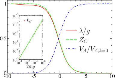
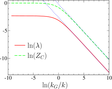
Figure 1: (Color online) Top panel: $\lambda/g$, $Z_{C}$ and $V_{A}/V_{A,k=0}$ vs $\ln(k_{G}/k)$ where $k_{G}=\sqrt{(gm)^{3}\bar{n}}/4\pi$, for $\bar{n}=0.01$, $2mg=0.1$ and $d=2$ [$\ln(k_{G}/k_{h})\simeq-5.87$]. The inset shows $k_{G}$ vs $2mg$ obtained from the criterion $V_{A,k_{G}}=V_{A,k=0}/2$ [the green solid line is a fit to $k_{G}\propto(2mg)^{3/2}$]. Bottom panel: $\ln(\lambda)$ and $\ln(Z_{C})$ vs $\ln(k_{G}/k)$. $\lambda$ and $Z_{C}$ vanish as $k$ for $k\ll k_{G}$ (blue dotted lines). All figures are obtained with $\Lambda=2m=1$ and the regulator (17).

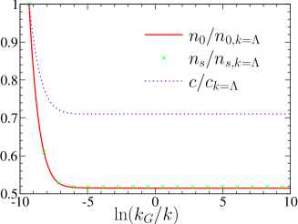
Figure 2: (Color online) Condensate density $n_{0}$, superfluid density $n_{s}=Z_{A}n_{0}=\bar{n}$ and Goldstone mode velocity $c$ vs $\ln(k_{G}/k)$. The parameters are the same as in Fig. 1.

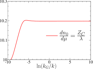
Figure 3: (Color online) Condensate compressibility $dn_{0}/d\mu=Z_{C}/\lambda$ vs $\ln(k_{G}/k)$ [Eq. (39)].

The flow of $\lambda$, $Z_{C}$ and $V_{A}$ is shown in Fig. 1. (The asymptotic behavior of various quantities as a function of the space dimension is summarized in table 1.) In agreement with the discussion of Secs. III and IV, we find that $\lambda,Z_{C}\sim k$ are suppressed as $k\to 0$, while $V_{A}$ flows toward a finite value. The anomalous self-energy $\Sigma_{\rm an}(p=0)=n_{0}\bar{\Gamma}_{B}(0)=n_{0}\lambda$ therefore vanishes for $k\to 0$ in agreement with the exact result Nepomnyashchii and Nepomnyashchii (1975). From Fig. 1, one can clearly identify the momentum scale $k_{G}$ below which the Bogoliubov approximation breaks down. The inset in the figure shows $k_{G}$ obtained from the criterion $V_{A,k_{G}}=V_{A,k=0}/2$. It is proportional to $\sqrt{(gm)^{3}\bar{n}}\sim gmk_{h}\ll k_{h}$, in agreement with the perturbative estimate (10). In practice, we use the definition $k_{G}=\sqrt{(gm)^{3}\bar{n}}/4\pi$. Note that the healing scale $k_{h}=\sqrt{2mg\bar{n}}$ (defined in Appendix A) keeps its mean-field (Bogoliubov) expression since the renormalization of the two-point vertex is very small for $k\sim k_{h}\gg k_{G}$.

Fig. 2 shows the behavior of the thermodynamic quantities $n_{0}$, $n_{s}$ and $c$. Since $Z_{A,k=0}\simeq 1.004$, the mean boson density $\bar{n}=Z_{A}n_{0}$ is nearly equal to the condensate density $n_{0}$. The condensate compressibility $dn_{0}/d\mu=Z_{C}/\lambda$ [Eq. (39)] is shown in Fig. 3. Apart from an initial variation at the beginning of the flow ($k\lesssim k_{h}$), these quantities do not vary with $k$. In particular, they are not sensitive to the Ginzburg scale $k_{G}$. This result is particularly remarkable for the Goldstone mode velocity $c$, whose expression (32) involves the parameters $\lambda$, $Z_{C}$ and $V_{A}$, which all strongly vary when $k\sim k_{G}$. These findings are a nice illustration of the fact that the divergence of the longitudinal susceptibility does not affect local gauge invariant quantities Pistolesi et al. (2004).

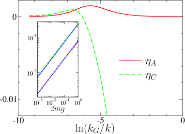
Figure 4: (Color online) $\eta_{A}$ and $\eta_{C}$ vs $\ln(k_{G}/k)$. The inset shows the location of the maxima in the curves $\eta_{A}$ (red crosses) and $\eta_{C}$ (green stars) vs $2mg$ [the blue solid lines correspond to ${\rm const}\times\sqrt{2mg\bar{n}}\propto k_{h}$]. The parameters are the same as in Fig. 2.

In Fig. 4 we show the flow of $\eta_{A}=-\partial_{t}\ln Z_{A}$ and $\eta_{C}=-\partial_{t}\ln Z_{C}$ for $k>k_{G}$. Both $\eta_{A}$ and $\eta_{C}$ exhibit a maximum corresponding to a slight increase of $Z_{A}$ and $Z_{C}$ ($Z_{A}$ then saturates to $Z_{A,k=0}$ while $Z_{C}$ strongly decreases when $k\sim k_{G}$). The location of these maxima is given by the healing scale $k_{h}$ (see inset in Fig. 4) not (e). The maxima of $\eta_{A}$ and $\eta_{C}$ become more pronounced as $2mg$ increases, but remains very small in the weak coupling limit $2mg\lesssim 1$. The small window around $k_{h}$ where the anomalous dimension $\eta_{A}$ is finite is likely to be a remnant of the critical regime that exists near the Goldstone regime at higher temperatures, and which is progressively suppressed as the temperature decreases.

V.1 Self-energies

The self-energies are obtained from the numerical solution of the flow equations (62) or (120). By computing $\bar{\Delta}_{\alpha}({\bf p},i\omega)$ for $N$ frequency points $i\omega_{l}$ ($l=1,\cdots,N$ with typically $N\sim 100$), one can construct a $N$-point Padé approximant $P_{\alpha}({\bf p},z)$ which is equal to $\bar{\Delta}_{\alpha}({\bf p},i\omega)$ when the complex frequency $z$ coincides with one of the Matsubara frequencies $i\omega_{l}$. The retarded part of the self-energy is then approximated by $\bar{\Delta}^{R}_{\alpha}({\bf p},\omega)=P_{\alpha}({\bf p},\omega+i0^{+})$ Vidberg and Serene (1977). (All self-energies discussed in this section corresponds to $k=0$.)

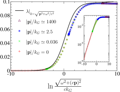
Figure 5: (Color online) $\bar{\Gamma}_{B,k=0}({\bf p},i\omega)=\bar{\Delta}_{B,k=0}({\bf p},i\omega)$ (symbols) and $\lambda_{k=\sqrt{{\bf p}^{2}+\omega^{2}/c^{2}}}$ (solid line) vs $\sqrt{\omega^{2}+(c{\bf p})^{2}}$ for various values of $|{\bf p}|$. The inset shows $\ln(\bar{\Gamma}_{B,k=0})$ and a fit to $C\sqrt{\omega^{2}+(c{\bf p})^{2}}$ (solid line).

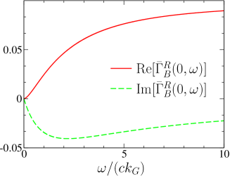
Figure 6: (Color online) Real and imaginary parts of the retarded vertex $\bar{\Gamma}^{R}_{B,k=0}({\bf p}=0,\omega)$ vs $\omega/(ck_{G})$.

Let us first discuss the momentum and frequency dependence of $\bar{\Delta}_{B}(p)$ at $k=0$. Note that $\bar{\Delta}_{B}(p)=\bar{\Gamma}_{B}(p)=\Sigma_{\rm an}(p)/n_{0}$ since $\lambda_{k=0}=0$. In the following, we shall rather discuss $\bar{\Gamma}_{B}(p)$ which is the right quantity to consider when comparing to the Bogoliubov approximation. Fig. 5 shows that $\bar{\Gamma}_{B}(p)$ is a function of $\omega^{2}+(c{\bf p})^{2}$, not only in the infrared regime $\sqrt{{\bf p}^{2}+\omega^{2}/c^{2}}\ll k_{G}$ but also for $\sqrt{{\bf p}^{2}+\omega^{2}/c^{2}}>k_{G}$. Furthermore, $\bar{\Gamma}_{B}(p)$ is related to the running coupling constant $\lambda_{k}$ by

$$\bar{\Gamma}_{B}(p)\simeq\lambda|_{k=\sqrt{{\bf p}^{2}+\omega^{2}/c^{2}}}.$$ (76)

This confirms that $\bar{\Gamma}_{B}(p)$ can be (approximately) obtained from $\bar{\Gamma}_{B,k}(p=0)$ by stopping the flow at $k\sim\sqrt{{\bf p}^{2}+\omega^{2}/c^{2}}$. For $\sqrt{{\bf p}^{2}+\omega^{2}/c^{2}}\gg k_{G}$, one therefore recovers the Bogoliubov result $\bar{\Gamma}_{B}(p)\simeq g$, while for $\sqrt{{\bf p}^{2}+\omega^{2}/c^{2}}\ll k_{G}$ one obtains

$$\bar{\Gamma}_{B}(p)\simeq C\sqrt{\omega^{2}+(c{\bf p})^{2}},$$ (77)

with $C$ a ${\bf p}$-independent constant.

Figure 7: (Color online) Real and imaginary parts of the retarded vertex $\bar{\Gamma}^{R}_{B,k=0}({\bf p},\omega)=\Sigma^{R}_{\rm an}({\bf p},\omega)/n_{0}$ for various values of $|{\bf p}|$ ranging from $0.3k_{G}$ up to $170k_{G}\sim k_{h}/2$ ($\bar{n}=0.01$ and $2mg=0.1$). The Bogoliubov approximation corresponds to $\bar{\Gamma}_{B}^{R}({\bf p},\omega)=g=0.1$. ($\Re[\bar{\Gamma}_{B}^{R}]\geq 0$ and $\Im[\bar{\Gamma}_{B}^{R}]\leq 0$.)

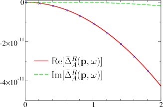
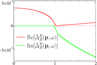
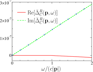
Figure 8: (Color online) Real and imaginary parts of the retarded self-energies $\bar{\Delta}^{R}_{A}({\bf p},\omega)$, $\bar{\Delta}^{R}_{B}({\bf p},\omega)=\bar{\Gamma}^{R}_{B}({\bf p},\omega)$ and $\bar{\Delta}^{R}_{C}({\bf p},\omega)$ for $|{\bf p}|\simeq 0.036k_{G}$ and $k=0$. The blue crosses correspond to the expressions (79) obtained from the derivative expansion, while the dotted lines show the analytical result (78) obtained from the approximation (77).

The Ginzburg scale $k_{G}$ manifests itself also in the frequency dependence of the retarded vertex $\bar{\Gamma}^{R}_{B}({\bf p}=0,\omega)$ (Fig. 6). For $|\omega|\gg ck_{G}$, the imaginary part $\Im[\bar{\Gamma}^{R}_{B}(0,\omega)]$ is very small and the real part tends to $g$ in agreement with the Bogoliubov approximation and the exact high-frequency limit (Appendix E). But for $|\omega|\ll ck_{G}$, the real part is strongly suppressed and becomes of the same order as the imaginary part. The crossover between the Bogoliubov and the infrared regimes can also be observed by varying $|{\bf p}|$ (Fig. 7). While the Bogoliubov result $\bar{\Gamma}^{R}_{B}({\bf p},\omega)=g$ is a good approximation when $|{\bf p}|\gg k_{G}$, $\bar{\Gamma}^{R}_{B}({\bf p},\omega)$ develops a strong frequency dependence for $|{\bf p}|\lesssim k_{G}$. For $|{\bf p}|\ll k_{G}$, we can use (77) to obtain the low-frequency behavior ($|\omega|\ll ck_{G}$)

$$\bar{\Gamma}^{R}_{B}({\bf p},\omega)\simeq{} C\sqrt{-(\omega+i0^{+})^{2}+(c{\bf p})^{2}}$$

$$\simeq{} C\theta(c|{\bf p}|-|\omega|)\sqrt{(c{\bf p})^{2}-\omega^{2}}$$

$$-iC{\rm sgn}(\omega)\theta(|\omega|-c|{\bf p}|)\sqrt{\omega^{2}-(c{\bf p})^{2}}$$ (78)

($\theta(x)$ is the step function). The Bogoliubov result $\bar{\Gamma}_{B}^{R}({\bf p},\omega)=g$ is nevertheless reproduced for $|\omega|\gg ck_{G}$ (Fig. 6). As shown in Fig. 8, the square-root singularity (78) is also obtained from the numerical result based on the Padé approximant. The asymptotic result (78) was first obtained by NN within a diagrammatic approach, and later reproduced by Popov and Seredniakov in the hydrodynamic approach Popov and Seredniakov (1979). Fig. 8 also shows the numerical results for $\bar{\Delta}_{A}^{R}({\bf p},\omega)$ and $\bar{\Delta}^{R}_{C}({\bf p},\omega)$. In the infrared regime $|{\bf p}|,|\omega|/c\ll k_{G}$, these self-energies are very well approximated by their derivative expansion,

$$\begin{split}\bar{\Delta}^{R}_{A}({\bf p},\omega)&\simeq-V_{A}\omega^{2}+(Z_{A}-1)\epsilon_{\bf p},\\ \bar{\Delta}^{R}_{C}({\bf p},\omega)&\simeq i\omega,\end{split}$$ (79)

where $V_{A}\equiv V_{A,k=0}$ and $Z_{A}\equiv Z_{A,k=0}$. The leading correction to $\bar{\Delta}^{R}_{C}({\bf p},\omega)\simeq i\omega$ is given by the relation (75) between $\bar{\Gamma}_{B}(p)$ and $\bar{\Gamma}_{C}(p)$, which is rather well satisfied when $|{\bf p}|,|\omega|/c\ll k_{G}$ (Fig. 9)

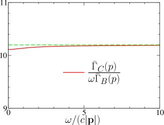
Figure 9: (Color online) $\bar{\Gamma}_{C}(p)/(\omega\bar{\Gamma}_{B}(p))$ vs $\omega/(c|{\bf p}|)$ for $|{\bf p}|\simeq 0.036k_{G}$ and $k=0$. The dashed line shows the value of $dn_{0}/d\mu|_{k=0}=\lim_{k\to 0}Z_{C}/\lambda$.

The imaginary part of $\bar{\Delta}_{A}^{R}$ and the real part of $\bar{\Delta}_{C}^{R}$ give a finite life-time to the sound mode. They arise from the decay of a phonon with momentum ${\bf p}$ into two phonons with momenta ${\bf q}$ and ${\bf p}-{\bf q}$ (Beliaev damping Beliaev (1958b)). This damping process follows from the second contribution (proportional to $\bar{\Gamma}^{(3)}\bar{\Gamma}^{(3)}$) to $\partial_{t}\bar{\Gamma}^{(2)}$ [Eq. (56)]. Fig. 10 shows that $\Im[\bar{\Delta}_{A}^{R}({\bf p},\omega)]$ and $\Re[\bar{\Delta}_{C}^{R}({\bf p},\omega)]$ vanish for $|\omega|\lesssim c|{\bf p}|$. The absence of damping below the threshold frequency $\sim c|{\bf p}|$ is due to the energy conservation $\omega=c|{\bf q}|+c|{\bf p}-{\bf q}|$ in the decay process. While it appears difficult to decide from the numerical results whether $\Im[\bar{\Delta}_{A}^{R}({\bf p},c|{\bf p}|)]$ and $\Re[\bar{\Delta}_{C}^{R}({\bf p},c|{\bf p}|)]$ (which determine the life-time of a phonon with momentum ${\bf p}$ and energy $c|{\bf p}|$) are zero or not, it is well known that for quasi-particles with a linear spectrum, Beliaev damping cannot take place as there is no phase space available Lifshitz_stat_phys_II . Beliaev damping requires a positive curvature of the quasi-particle dispersion, i.e. $E_{\bf p}=c|{\bf p}|+a|{\bf p}|^{3}$ ($a>0$). In this case, the threshold frequency, obtained from the condition $\omega=E_{\bf q}+E_{{\bf p}-{\bf q}}$ (with ${\bf p}$ fixed), lies below $E_{\bf p}$. The decay of a quasi-particle into a pair of quasi-particles then gives a scattering rate of order $|{\bf p}|^{3}$ in a two-dimensional system Kreisel et al. (2008); Chung and Bhattacherjee . Since we use the derivative expansion of the vertices to compute the self-energies $\bar{\Delta}_{\alpha}^{R}$ (see Sec. IV), the quasi-particle dispersion becomes linear to a very high degree of accuracy in the “relativistic” regime $|{\bf p}|\ll k_{G}$. In this regime, we expect the curvature of the dispersion to originate in the $({\bf p},\omega)$ dependence of the self-energy $\bar{\Delta}_{A}^{R}({\bf p},\omega)$ that is not included in the derivative expansion. Thus a reliable computation of the Beliaev damping would require a self-consistent numerical solution of the flow equations.

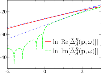
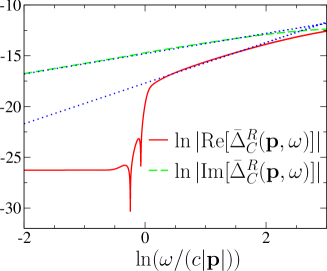
Figure 10: (Color online) Real and imaginary parts of the retarded self-energies $\bar{\Delta}_{A}^{R}({\bf p},\omega)$ and $\bar{\Delta}_{A}^{R}({\bf p},\omega)$. For $\omega\gtrsim c|{\bf p}|$, $\Re[\bar{\Delta}_{A}^{R}({\bf p},\omega)]\sim\omega^{2}$, $\Im[\bar{\Delta}_{A}^{R}({\bf p},\omega)]\sim\omega^{3}$, $\Re[\bar{\Delta}_{C}^{R}({\bf p},\omega)]\sim\omega^{2}$, $\Im[\bar{\Delta}_{C}^{R}({\bf p},\omega)]\sim\omega$ (blue dotted lines). The spikes are due to $\Im[\bar{\Delta}_{A}^{R}({\bf p},\omega)]$ and $\Re[\bar{\Delta}_{C}^{R}({\bf p},\omega)]$ being nearly zero and changing sign.

While the Padé approximant technique is very efficient to obtain $\bar{\Delta}_{B}^{R}({\bf p},\omega)$, as well as $\bar{\Delta}^{R}_{A}({\bf p},\omega)$ and $\bar{\Delta}_{C}^{R}({\bf p},\omega)$ in the infrared regime, the computation of $\bar{\Delta}^{R}_{A}({\bf p},\omega)$ and $\bar{\Delta}_{C}^{R}({\bf p},\omega)$ for $|{\bf p}|\gg k_{G}$ appears more difficult for reasons that we do not fully understand. (Note also that the use of the derivative expansion might also be a source of difficulties for reasons discussed in Sec. IV.2.) In the limit $|{\bf p}|\gg k_{G}$, the Bogoliubov approximation is however essentially correct and the corrections $\bar{\Delta}^{R}_{A}({\bf p},\omega)$ and $\bar{\Delta}_{C}^{R}({\bf p},\omega)$ provide a small broadening of the Bogoliubov quasi-particles (Beliaev damping) as can be directly verified from the one-loop self-energy diagrams.

V.2 Spectral functions

The knowledge of the retarded one-particle Green function enables to compute the spectral functions not (f)

$$\begin{split}A_{\rm ll}({\bf p},\omega)&=-\frac{1}{\pi}\Im[\bar{G}_{\rm ll}^{R}({\bf p},\omega)],\\ A_{\rm tt}({\bf p},\omega)&=-\frac{1}{\pi}\Im[\bar{G}_{\rm tt}^{R}({\bf p},\omega)],\\ A_{\rm lt}({\bf p},\omega)&=\frac{i}{\pi}\Re[\bar{G}_{\rm lt}^{R}({\bf p},\omega)].\end{split}$$ (80)

From equations (47) and (48), we obtain

$$\begin{split}A_{\rm tt}({\bf p},\omega)&=\frac{mcn_{0}}{\bar{n}|{\bf p}|}[\delta(\omega-c|{\bf p}|)-\delta(\omega+c|{\bf p}|)],\\ A_{\rm ll}({\bf p},\omega)&=\frac{{\rm sgn}(\omega)}{2\pi n_{0}C}\frac{\theta(|\omega|-c|{\bf p}|)}{\sqrt{\omega^{2}-(c{\bf p})^{2}}},\\ A_{\rm lt}({\bf p},\omega)&=i\frac{mc^{2}}{2\bar{n}}\frac{dn_{0}}{d\mu}[\delta(\omega-c|{\bf p}|)+\delta(\omega+c|{\bf p}|)],\end{split}$$ (81)

in the infrared regime. $A_{\rm tt}({\bf p},\omega)$ and $A_{\rm lt}({\bf p},\omega)$ exhibit Dirac peaks at the sound mode energy $\pm c|{\bf p}|$. On the other hand, the longitudinal spectral function $A_{\rm ll}({\bf p},\omega)$ shows a critical continuum with a singularity at the Bogoliubov mode energy, in agreement with the predictions of the hydrodynamic approach Giorgini et al. (1992). The spectral function $A_{\rm ll}({\bf p},\omega)$ obtained from the Padé approximant is shown in Fig. 11. The square root singularity is very well reproduced and extends up to $\omega\sim ck_{G}$.

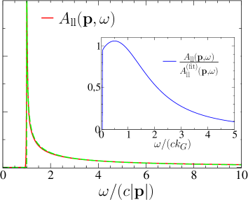
Figure 11: (Color online) Spectral function $A_{\rm ll}({\bf p},\omega)$ for $|{\bf p}|\simeq 0.036k_{G}$ and $k=0$. The red solid line is the result obtained from the Padé approximant, while the green dashed line corresponds to the analytic expression in (81). The inset shows the ratio between $A_{\rm ll}({\bf p},\omega)$ and the approximate result (81) on a larger energy scale.

From these results, we can deduce the spectral function of the normal (U(1) invariant) Green function (see Appendix E),

$$A_{\rm n}({\bf p},\omega) =-\frac{1}{\pi}\Im[G_{\rm n}^{R}({\bf p},\omega)]$$

$$=\frac{1}{2}\left[A_{\rm ll}({\bf p},\omega)+A_{\rm tt}({\bf p},\omega)\right]-iA_{\rm lt}({\bf p},\omega)$$

$$\simeq\frac{1}{2}\left[A_{\rm ll}({\bf p},\omega)+A_{\rm tt}({\bf p},\omega)\right].$$ (82)

The singularity of the longitudinal correlation function shows up as a continuum of excitations above the Bogoliubov sound mode. The respective spectral weights at positive frequencies of the transverse and longitudinal fluctuations are given by

$$\begin{split}S_{\rm tt}&=\frac{mcn_{0}}{2\bar{n}|{\bf p}|},\\ S_{\rm ll}&\simeq\frac{1}{4\pi n_{0}C}\int_{c|{\bf p}|}^{ck_{G}}\frac{d\omega}{\sqrt{\omega^{2}-(c{\bf p})^{2}}}\\ &\simeq\frac{1}{4\pi n_{0}C}\ln\left(\frac{2k_{G}}{|{\bf p}|}\right)\end{split}$$ (83)

for $|{\bf p}|\ll k_{G}$. Using the estimate (49) of the constant $C$, we obtain the ratio

$$\begin{split}\frac{S_{\rm ll}}{S_{\rm tt}}&\simeq\frac{mc|{\bf p}|}{8\pi\bar{n}}\ln\left(\frac{2k_{G}}{|{\bf p}|}\right)\\ &\simeq\frac{1}{8\pi}\left(\frac{mg}{\bar{n}}\right)^{1/2}|{\bf p}|\ln\left(\frac{2k_{G}}{|{\bf p}|}\right),\end{split}$$ (84)

where the last result is obtained with $c\simeq\sqrt{g\bar{n}/m}$. This ratio is extremely small in the weak coupling limit where $mg\ll 1$ and $|{\bf p}|\ll k_{G}\ll\sqrt{\bar{n}}$. It can however become sizable in the intermediate coupling regime when $mg\sim 1$ and $k_{G}$ is not much smaller than $\sqrt{\bar{n}}$.

VI Conclusion

The BMW NPRG method provides a powerful tool to study interacting boson systems. In particular, it enables to obtain the momentum and frequency dependence of the correlation functions on all energy scales. Our results reveal the crucial role of the Ginzburg scale $k_{G}$ in zero-temperature Bose superfluids. At large momenta or energies, $|{\bf p}|\gg k_{G}$ or $|\omega|/c\gg k_{G}$, the Bogoliubov theory provides a good approximation to the correlation functions. For $|{\bf p}|,|\omega|/c\ll k_{G}$, the correlation functions are governed by a different fixed point, which corresponds to Popov’s hydrodynamic theory. Throughout the paper, we have emphasized that interacting boson systems can be understood within the framework of the (quantum) $O(2)$ model. The infrared behavior of this model is characterized by singular longitudinal fluctuations induced by the coupling to transverse (phase) fluctuations, a phenomenon which is common to all models with a continuous broken symmetry Patasinskij and Pokrovskij (1973).

From a technical point, we have not solved the BMW equations in their full glory. By neglecting the field dependence of the self-energies $\Delta_{\alpha}(p;n)$ (which were approximated by $\Delta_{\alpha}(p;n_{0})$) and using the derivative expansion, we have obtained flow equations which can be solved with reasonable numerical effort. Yet these equations yield a remarkable description of the singularity of the self-energy induced by the divergence of the longitudinal susceptibility. Quasi-particle life-time (Beliaev damping) can also be obtained in principle if the flow equations are solved self-consistently (i.e. without relying on the derivative expansion).

We have restricted our analysis to the weak coupling limit where the two characteristic momentum scales $k_{h}$ and $k_{G}$ are well separated ($k_{G}\ll k_{h}\ll\bar{n}^{1/d}$). The characteristic momentum scale $\bar{n}^{1/d}$ does not play any role in this limit. When the dimensionless coupling constant is of order unity (intermediate coupling regime), the three characteristic scales become of the same order: $k_{G}\sim k_{h}\sim\bar{n}^{1/d}$. The momentum range $[k_{G},k_{h}]$ where the linear spectrum can be described by the Bogoliubov theory is then suppressed. We expect the strong coupling regime to be governed by a single characteristic momentum scale, namely $\bar{n}^{1/d}$. A good description of physical phenomena at the scale of the interparticle spacing is likely to require the consideration of the complete BMW equations (with no additional approximation) with both the field and $({\bf p},\omega)$ dependence of the vertices taken into account.

In one dimension, superfluidity exists without Bose Einstein condensation ($n_{0}=0$), and our results regarding the infrared behavior of the correlation functions do not apply. If however, we insist on using the Bogoliubov theory as a starting point, we find from the perturbative estimate of Sec. A.3 a characteristic length $k_{G}\sim(gm)^{3/4}n_{0}^{1/4}$. This expression makes sense if we interpret $n_{0}$ as the condensate density $n_{0,k_{G}}$ at the scale $k_{G}$. A similar characteristic scale, $k_{s}\sim(gm)^{3/4}\bar{n}^{1/4}$, has been found in Ref. Khodas et al. . In weakly interacting one-dimensional Bose gases, $k_{s}$ separates a high-momentum regime ($|{\bf p}|>k_{s}$) where the Gross-Pitaevskii description is valid, from a low-momentum regime ($|{\bf p}|<k_{s}$) where a more elaborate description (e.g. based on the exact solution of the Lieb-Liniger model Lieb and Liniger (1963); Lieb (1963)) is required. The description of one-dimensional superfluidity from the NPRG is challenging, even if the derivative expansion yields reasonable results at weak coupling Dupuis and Sengupta (2007), and should be an interesting test of the BMW scheme.

Appendix A Bogoliubov’s theory

In this Appendix, we briefly review the main results of Bogoliubov’s theory.

A.1 Beliaev’s self-energies

The action of interacting bosons is often written in terms of the two-component field

$$\Psi(p)=\left(\begin{array}[]{c}\psi(p)\\ \psi^{*}(-p)\end{array}\right),\quad\Psi^{\dagger}(p)=\bigl{(}\psi^{*}(p),\psi(-p)\bigr{)},$$ (85)

where $p=({\bf p},i\omega)$. The one-particle (connected) propagator then becomes a $2\times 2$ matrix whose inverse in Fourier space is given by

$$\left(\begin{array}[]{cc}i\omega+\mu-\epsilon_{\bf p}-\Sigma_{\rm n}(p)&-\Sigma_{\rm an}(p)\\ -\Sigma_{\rm an}^{*}(p)&-i\omega+\mu-\epsilon_{\bf p}-\Sigma_{\rm n}(-p)\end{array}\right),$$ (86)

where $\Sigma_{\rm n}$ and $\Sigma_{\rm an}$ are the normal and anomalous self-energies, respectively, and $\epsilon_{\bf p}={\bf p}^{2}/2m$. Making use of (14) and the relation $G=-\bar{\Gamma}^{(2)-1}$ between the propagator and the two-point vertex, one obtains equation (27) if one chooses a real order parameter $\langle\psi(x)\rangle=\sqrt{n_{0}}$. The normal and anomalous self-energies satisfy the Hugenholtz-Pines theorem Hugenholtz and Pines (1959)

$$\Sigma_{\rm n}(0)-\Sigma_{\rm an}(0)=\mu,$$ (87)

which is a consequence of the spontaneously broken global U(1) symmetry in the superfluid phase.

Using (86), we can relate the longitudinal propagator

$$G_{\rm ll}(p) =-\langle\psi_{1}(p)\psi_{1}(-p)\rangle_{c}$$

$$=-\frac{1}{2}\langle[\psi(p)+\psi^{*}(-p)][\psi(-p)+\psi^{*}(p)]\rangle_{c}$$ (88)

($\langle\cdots\rangle_{c}$ denotes for the connected part of the propagator) to the self-energies $\Sigma_{\rm n}$ and $\Sigma_{\rm an}$. Anticipating that $\mu-\Sigma_{\rm n}(p),\Sigma_{\rm an}(p)\gg{\bf p}^{2},\omega^{2}$ when ${\bf p},\omega\to 0$ (and neglecting terms ${\cal O}({\bf p}^{2},\omega^{2})$, we deduce

$$\lim_{p\to 0}G_{\rm ll}(p) =\lim_{p\to 0}\frac{\mu-\frac{1}{2}[\Sigma_{\rm n}(p)+\Sigma_{\rm n}(-p)]+\Sigma_{\rm an}(p)}{[\mu-\Sigma_{\rm n}(p)][\mu-\Sigma_{\rm n}(-p)]-\Sigma_{\rm an}(p)^{2}}$$

$$=\lim_{p\to 0}\frac{-1}{2\Sigma_{\rm an}(p)}$$

$$=\lim_{p\to 0}\frac{-1}{2n_{0}\bar{\Gamma}_{B}(p)},$$ (89)

where we have used the Hugenholtz-Pines theorem (87).

A.2 Bogoliubov’s approximation

The Bogoliubov approximation is based on the microscopic action (13) and a first-order computation of the self-energies

$$\begin{split}\Sigma_{\rm n}^{\rm B}(p)&=2gn_{0},\\ \Sigma_{\rm an}^{\rm B}(p)&=gn_{0},\end{split}$$ (90)

where the condensate density $n_{0}=\mu/g$. This yields the propagators

$$\begin{split}G_{\rm n}^{\rm B}(p)&=-\langle\psi(p)\psi^{*}(p)\rangle_{c}=\frac{-i\omega-\epsilon_{\bf p}-gn_{0}}{\omega^{2}+E_{\bf p}^{2}},\\ G_{\rm an}^{\rm B}(p)&=-\langle\psi(p)\psi(-p)\rangle_{c}=\frac{gn_{0}}{\omega^{2}+E_{\bf p}^{2}},\end{split}$$ (91)

where $E_{\bf p}=[\epsilon_{\bf p}(\epsilon_{\bf p}+2gn_{0})]^{1/2}$ is the Bogoliubov quasi-particle excitation energy. When $|{\bf p}|$ is larger than the healing momentum $k_{h}=(2gmn_{0})^{1/2}$, the spectrum $E_{\bf p}\simeq\epsilon_{\bf p}+gn_{0}$ is particle-like, whereas it becomes sound-like for $|{\bf p}|\ll k_{h}$ with a velocity $c_{B}=\sqrt{gn_{0}/m}$. In the small-momentum limit $|{\bf p}|\ll k_{h}$,

$$\begin{split}G^{\rm B}_{\rm ll}(p)&=-\frac{\epsilon_{\bf p}}{\omega^{2}+c_{B}^{2}{\bf p}^{2}},\\ G^{\rm B}_{\rm tt}(p)&=-\frac{2gn_{0}}{\omega^{2}+c_{B}^{2}{\bf p}^{2}},\\ G^{\rm B}_{\rm lt}(p)&=\frac{\omega}{\omega^{2}+c_{B}^{2}{\bf p}^{2}}.\end{split}$$ (92)

Note that in the Bogoliubov approximation, the occurrence of a linear spectrum is related to $\Sigma_{\rm an}(0)$ being nonzero. In the weak coupling limit, $n_{0}$ is approximately given by the full density $\bar{n}$, and the healing momentum can also be defined by $k_{h}=(2gm\bar{n})^{1/2}$ (which is the definition taken in Sec. V).

A.3 Perturbative estimate of the Ginzburg scale $k_{G}$

Let us consider the one-loop correction $\Sigma_{\rm an}^{(1)}(p)$ to the Bogoliubov result $\Sigma_{\rm an}^{B}(p)=gn_{0}$. The leading contribution comes from the one-loop diagram

where the internal lines correspond to transverse fluctuations, i.e.

$$\Sigma_{\rm an}^{(1)}(p) \simeq-\frac{g^{2}n_{0}}{2}\int_{q}G_{\rm tt}(q)G_{\rm tt}(p+q)$$

$$\simeq-\frac{g^{2}n_{0}}{2}\frac{S_{d}}{(2\pi)^{d}}\int_{k}^{k_{h}}d|{\bf q}||{\bf q}|^{d-1}$$

$$\hskip 56.9055pt\times\int_{-\infty}^{\infty}\frac{d\omega}{2\pi}\left(\frac{2gn_{0}}{\omega^{2}+c_{B}^{2}{\bf q}^{2}}\right)^{2}$$

$$\simeq-\frac{g}{2}(gmn_{0})^{3/2}\frac{S_{d}}{(2\pi)^{d}}\int_{k}^{k_{h}}\frac{d|{\bf q}|}{|{\bf q}|^{4-d}},$$ (93)

where $k_{h}$ is the healing momentum defined in section A.2, and $S_{d}$ the surface of the unit sphere in $d$ dimensions. The infrared limit $k$ in the integral is of order $({\bf p}^{2}+\omega_{\nu}^{2}/c_{B}^{2})^{1/2}$ (with $p=({\bf p},i\omega_{\nu})$). The one-loop correction is divergent when $d\leq 3$. This divergence reflects the difficulties of diagrammatic calculations beyond the Bogoliubov approximation and is a manifestation of the diverging longitudinal susceptibility Weichman (1988). We estimate the Ginzburg momentum scale $k_{G}$ from the condition $|\Sigma_{\rm an}^{(1)}(p)|\sim|\Sigma_{\rm an}^{B}(p)|$ [see Eq. (10)].

Appendix B Symmetries and Ward identities

B.1 Gauge invariance

Let us consider the microscopic action

$$S=\int dx \Bigl{[}\psi^{*}(x)\Bigl{(}{\partial_{\tau}}-\mu(x)-\frac{1}{2m}[\boldsymbol{\nabla}-i{\bf A}(x)]^{2}\Bigr{)}\psi(x)$$

$$+\frac{g}{2}|\psi(x)|^{4}\Bigr{]}$$ (94)

in the presence of external sources $\mu(x)$ and ${\bf A}(x)$. $S$ is invariant in the gauge transformation

$$\begin{split}\\ \psi(x)&\to\psi(x)e^{i\alpha(x)},\\ \psi^{*}(x)&\to\psi^{*}(x)e^{-i\alpha(x)},\\ \mu(x)&\to\mu(x)+i{\partial_{\tau}}\alpha(x)\\ {\bf A}(x)&\to{\bf A}(x)+\boldsymbol{\nabla}\alpha(x),\end{split}$$ (95)

where $\alpha(x)$ is an arbitrary real function. This implies that the effective action satisfies

$$\Gamma[R(\alpha)\phi,\mu+i{\partial_{\tau}}\alpha,A_{\nu}+\partial_{\nu}\alpha]=\Gamma[\phi,\mu,A_{\nu}],$$ (96)

where $\phi=(\phi_{1},\phi_{2})^{T}$ and

$$R(\alpha)=\left(\begin{array}[]{cc}\cos(\alpha)&-\sin(\alpha)\\ \sin(\alpha)&\cos(\alpha)\end{array}\right)$$ (97)

is a two-dimensional rotation matrix. Differentiating (96) with respect to $\alpha(x)$, we obtain

$$\sum_{i,j}\frac{\delta\Gamma}{\delta\phi_{i}(x)}\epsilon_{ij}\phi_{j}(x)+i{\partial_{\tau}}\frac{\delta\Gamma}{\delta\mu(x)}+\sum_{\nu}\partial_{\nu}\frac{\delta\Gamma}{\delta A_{\nu}(x)}=0.$$ (98)

Differentiating now with respect to $\phi_{l}(x_{2})$ and $\mu(x_{2})$ and setting $\phi=(\sqrt{2n_{0}},0)$, $\mu(x)=\mu$ and ${\bf A}(x)=0$ gives

$$\begin{split}-\sqrt{2n_{0}}\bar{\Gamma}^{(2)}_{l2}(x_{2},x_{1})&+i\partial_{\tau_{1}}\bar{\Gamma}^{(2)}_{l;0}(x_{2},x_{1})\\ &+\sum_{\nu_{1}}\partial_{\nu_{1}}\bar{\Gamma}^{(2)}_{l;\nu_{1}}(x_{2},x_{1})=0,\\ -\sqrt{2n_{0}}\bar{\Gamma}^{(2)}_{2;0}(x_{1},x_{2})&+i\partial_{\tau_{1}}\bar{\Gamma}^{(2)}_{;00}(x_{1},x_{2})\\ &+\sum_{\nu_{1}}\partial_{\nu_{1}}\bar{\Gamma}^{(2)}_{;\nu_{1}0}(x_{1},x_{2})=0,\end{split}$$ (99)

where we have introduced

$$\begin{split}\Gamma^{(2)}_{l;0}(x_{2},x_{1})&=\frac{\delta^{(2)}\Gamma}{\delta\phi_{l}(x_{2})\delta\mu(x_{1})},\\ \Gamma^{(2)}_{;00}(x_{2},x_{1})&=\frac{\delta^{(2)}\Gamma}{\delta\mu(x_{2})\delta\mu(x_{1})},\end{split}$$ (100)

and similar definitions for $\Gamma^{(2)}_{l;\nu}(x_{2},x_{1})$ and $\Gamma^{(2)}_{;\nu 0}(x_{2},x_{1})$. Note that with the choice $\phi=(\sqrt{2n_{0}},0)$, we can identify $\bar{\Gamma}_{12}^{(2)}$ to $\bar{\Gamma}_{C}$, and $\bar{\Gamma}_{22}^{(2)}$ to $\bar{\Gamma}_{A}$. In Fourier space, (99) leads to the Ward identities

$$\sqrt{2n_{0}}\bar{\Gamma}^{(2)}_{12}(p)+\omega\bar{\Gamma}^{(2)}_{1;0}(p)+\sum_{\nu}ip_{\nu}\bar{\Gamma}^{(2)}_{1;\nu}(p) =0,$$ (101)

$$\sqrt{2n_{0}}\bar{\Gamma}^{(2)}_{22}(p)+\omega\bar{\Gamma}^{(2)}_{2;0}(p)+\sum_{\nu}ip_{\nu}\bar{\Gamma}^{(2)}_{2;\nu}(p) =0,$$ (102)

$$\sqrt{2n_{0}}\bar{\Gamma}^{(2)}_{2;0}(p)-\omega\bar{\Gamma}^{(2)}_{;00}(p)-\sum_{\nu}ip_{\nu}\bar{\Gamma}^{(2)}_{;\nu 0}(p) =0.$$ (103)

From (101), we deduce

$$\frac{\partial}{\partial\omega}\bar{\Gamma}^{(2)}_{12}(p)\Bigl{|}_{p=0} =-\frac{1}{\sqrt{2n_{0}}}\bar{\Gamma}^{(2)}_{1;0}(p=0),$$

$$=-\frac{1}{\sqrt{2n_{0}}}\frac{\partial^{2}U}{\partial\phi_{1}\partial\mu}\biggl{|}_{n_{0}}=-\frac{\partial^{2}U}{\partial n\partial\mu}\biggl{|}_{n_{0}},$$ (104)

where the effective potential $U(n,\mu)$ is considered as a function of both $n$ and $\mu$. From (102) and (103), we obtain

$$\begin{split}\frac{\partial}{\partial\omega^{2}}\bar{\Gamma}^{(2)}_{22}(p)\Bigl{|}_{p=0}&=-\frac{1}{\sqrt{2n_{0}}}\frac{\partial}{\partial\omega}\bar{\Gamma}^{(2)}_{2;0}(p)\Bigl{|}_{p=0},\\ \frac{\partial}{\partial\omega}\bar{\Gamma}^{(2)}_{2;0}(p)\Bigl{|}_{p=0}&=\frac{1}{\sqrt{2n_{0}}}\bar{\Gamma}^{(2)}_{;00}(0)=\frac{1}{\sqrt{2n_{0}}}\frac{\partial^{2}U}{\partial\mu^{2}}\biggl{|}_{n_{0}}\end{split}$$ (105)

and therefore

$$\frac{\partial}{\partial\omega^{2}}\bar{\Gamma}^{(2)}_{22}(p)\Bigl{|}_{p=0}=-\frac{1}{2n_{0}}\frac{\partial^{2}U}{\partial\mu^{2}}\biggl{|}_{n_{0}}.$$ (106)

B.2 Galilean invariance

Another Ward identity can be obtained from the Galilean invariance of the microscopic action. The latter is invariant in the transformation $\psi(x)\to\psi(x)e^{i{\bf q}\cdot{\bf r}}$, $\psi^{*}(x)\to\psi(x)e^{-i{\bf q}\cdot{\bf r}}$ if we shift the chemical potential $\mu$ by ${\bf q}^{2}/2m$, which implies

$$\Gamma[R(\alpha)\phi,\mu+{\bf q}^{2}/2m]=\Gamma[\phi,\mu],$$ (107)

where $\alpha(x)={\bf q}\cdot{\bf r}$ and the chemical potential $\mu$ is taken uniform and time independent. To order ${\bf q}^{2}$, equation (107) gives

$$\begin{split}0&=\frac{{\bf q}^{2}}{2m}\frac{\partial\bar{\Gamma}}{\partial\mu}+n_{0}\int dxdx^{\prime}\bar{\Gamma}^{(2)}_{22}(x-x^{\prime})\alpha(x)\alpha(x^{\prime})\\ &=\frac{{\bf q}^{2}}{2m}\frac{\partial\bar{\Gamma}}{\partial\mu}+\beta Vn_{0}{\bf q}^{2}\frac{\partial}{\partial{\bf p}^{2}}\bar{\Gamma}^{(2)}_{22}(p)\Bigl{|}_{p=0},\end{split}$$ (108)

where we have set $\phi=(\sqrt{2n_{0}},0)$. Since

$$\frac{\partial\bar{\Gamma}}{\partial\mu}=\beta V\frac{\partial U}{\partial\mu}\biggl{|}_{n_{0}}=-\beta V\bar{n}$$ (109)

(see Eq. (37)), we finally obtain

$$\frac{\partial}{\partial{\bf p}^{2}}\bar{\Gamma}^{(2)}_{22}(p)\Bigl{|}_{p=0}=\frac{\bar{n}}{2mn_{0}},$$ (110)

where $\bar{n}$ is the mean boson density.

Appendix C Flow equations

C.1 BMW equations

In the BMW approximation, the flow equation of the two-point vertex is given by

$$\partial_{t}\Gamma^{(2)}_{ij}(p;\phi)=-\frac{1}{2}\sum_{q,i_{1},i_{2}}\tilde{\partial}_{t}G_{i_{1}i_{2}}(q;\phi)\Gamma^{(4)}_{iji_{2}i_{1}}(p,-p,0,0;\phi)\\ -\frac{1}{2}\sum_{q,i_{1}\cdots i_{4}}\Bigl{\{}\Gamma^{(3)}_{ii_{2}i_{3}}(p,0,-p;\phi)\Gamma^{(3)}_{ji_{4}i_{1}}(-p,p,0;\phi)[\tilde{\partial}_{t}G_{i_{1}i_{2}}(q;\phi)]G_{i_{3}i_{4}}(p+q;\phi)+(p\leftrightarrow-p,i\leftrightarrow j)\Bigr{\}},$$ (111)

where the three- and four-point vertices in (111) are obtained from the field derivatives of the two-point vertex [Eq. (57)]. From (21) and (44), we obtain

$$\begin{split}G_{ij}(p;\phi)={}&\delta_{i,j}[\delta_{i,1}G_{\rm ll}(p;n)+\delta_{i,2}G_{\rm tt}(p;n)]+\epsilon_{ij}G_{\rm lt}(p;n),\\ \Gamma^{(2)}_{ij}(p;\phi)={}&\delta_{i,j}[\Gamma_{A}(p;n)+\delta_{i,1}2n\Gamma_{B}(p;n)]+\epsilon_{ij}\Gamma_{C}(p;n),\\ \Gamma^{(3)}_{ijl}(p,-p,0;\phi)={}&\frac{\sqrt{2n}}{\sqrt{\beta V}}\Bigl{\{}\delta_{i,j}\delta_{l,1}\bigl{[}\Gamma_{A}^{\prime}(p;n)+\delta_{i,1}2n\Gamma_{B}^{\prime}(p;n)\bigr{]}+(\delta_{i,l}\delta_{j,1}+\delta_{j,l}\delta_{i,1})\Gamma_{B}(p;n)+\epsilon_{ij}\delta_{l,1}\Gamma_{C}^{\prime}(p;n)\Bigr{\}},\\ \Gamma^{(4)}_{ijlm}(p,-p,0,0;\phi)={}&\frac{1}{\beta V}\Bigl{\{}\delta_{i,j}\delta_{l,m}\bigl{[}\Gamma^{\prime}_{A}(p;n)+\delta_{l,1}2n\Gamma^{\prime\prime}_{A}(p;n)\bigr{]}+(\delta_{i,l}\delta_{j,m}+\delta_{j,l}\delta_{i,m})\Gamma_{B}(p;n)\\ &+\bigl{[}\delta_{i,1}(\delta_{j,m}\delta_{l,1}+\delta_{l,m}\delta_{j,1})+\delta_{m,1}(\delta_{i,l}\delta_{j,1}+\delta_{j,l}\delta_{i,1})+\delta_{i,m}\delta_{j,1}\delta_{l,1}\bigr{]}2n\Gamma^{\prime}_{B}(p;n)\\ &+\delta_{i,1}\delta_{j,1}\delta_{l,1}\delta_{m,1}4n^{2}\Gamma^{\prime\prime}_{B}(p;n)+\delta_{l,m}\epsilon_{ij}\bigl{[}\Gamma^{\prime}_{C}(p;n)+\delta_{l,1}2n\Gamma^{\prime\prime}_{C}(p;n)\bigr{]}\Bigl{\}}\end{split}$$ (112)

($\Gamma_{\alpha}^{\prime}(p;n)=\partial_{n}\Gamma_{\alpha}(p;n)$, etc.) for the particular field configuration $\phi=(\sqrt{2n},0)$. The flow equation (111) then gives

$$\partial_{t}\Gamma_{A}(p;n)={} -\frac{1}{2}I_{\rm ll}(n)[\Gamma^{\prime}_{A}(p;n)+2n\Gamma^{\prime\prime}_{A}(p;n)]-\frac{1}{2}I_{\rm tt}(n)[\Gamma^{\prime}_{A}(p;n)+2\Gamma_{B}(p;n)]$$

$$-2n\bigl{[}J_{\rm ll,tt}(p;n)\Gamma_{A}^{\prime}(p;n)^{2}+J_{\rm tt,ll}(p;n)\Gamma_{B}(p;n)^{2}+2J_{\rm lt,lt}(p;n)\Gamma^{\prime}_{A}(p;n)\Gamma_{B}(p;n)$$

$$-J_{\rm ll,ll}(p;n)\Gamma^{\prime}_{C}(p;n)^{2}-2J_{\rm ll,lt}(p;n)\Gamma_{A}^{\prime}(p;n)\Gamma^{\prime}_{C}(p;n)+2J_{\rm lt,ll}(p;n)\Gamma_{B}(p;n)\Gamma^{\prime}_{C}(p;n)\bigl{]},$$ (113)

$$\partial_{t}\Gamma_{B}(p;n)={} \frac{1}{2n}[I_{\rm tt}(n)-I_{\rm ll}(n)]\Gamma_{B}(p;n)-I_{\rm ll}(n)\left[\frac{5}{2}\Gamma^{\prime}_{B}(p;n)+n\Gamma^{\prime\prime}_{B}(p;n)\right]-\frac{1}{2}I_{\rm tt}(n)\Gamma^{\prime}_{B}(p;n)$$

$$-J_{\rm ll,ll}(p;n)\bigl{[}X(n)^{2}+\Gamma^{\prime}_{C}(p;n)^{2}\bigr{]}+J_{\rm ll,tt}(p;n)\bigl{[}\Gamma^{\prime}_{A}(p;n)^{2}+\Gamma^{\prime}_{C}(p;n)^{2}\bigr{]}+J_{\rm tt,ll}(p;n)\Gamma_{B}(p;n)^{2}$$

$$-J_{\rm tt,tt}(p;n)\Gamma_{B}(p;n)^{2}+2J_{\rm lt,lt}(p;n)\Gamma_{B}(p;n)\bigl{[}X(n)+\Gamma^{\prime}_{A}(p;n)\bigr{]}+2J_{\rm ll,lt}(p;n)\bigl{[}X(n)-\Gamma^{\prime}_{A}(p;n)\bigr{]}\Gamma^{\prime}_{C}(p;n)$$

$$+2J_{\rm lt,ll}(p;n)\Gamma_{B}(p;n)\Gamma^{\prime}_{C}(p;n)+2J_{\rm lt,tt}(p;n)\Gamma_{B}(p;n)\Gamma^{\prime}_{C}(p;n),$$ (114)

$$\partial_{t}\Gamma_{C}(p;n)={} -\frac{1}{2}I_{\rm ll}(n)\bigl{[}\Gamma^{\prime}_{C}(p;n)+2n\Gamma^{\prime\prime}_{C}(p;n)\bigr{]}-\frac{1}{2}I_{\rm tt}(n)\Gamma^{\prime}_{c}(p;n)$$

$$-2n\Bigl{\{}J_{\rm ll,ll}(p;n)X(n)\Gamma^{\prime}_{C}(p;n)+J_{\rm ll,tt}(p;n)\Gamma^{\prime}_{A}(p;n)\Gamma^{\prime}_{C}(p;n)-J_{\rm tt,lt}(p;n)\Gamma_{B}(p;n)^{2}$$

$$+J_{\rm lt,ll}(p;n)\Gamma_{B}(p;n)\Gamma^{\prime}_{A}(p;n)+J_{\rm ll,lt}(p;n)\bigl{[}X(n)\Gamma^{\prime}_{A}(p;n)-\Gamma^{\prime}_{C}(p;n)^{2}\bigr{]}-J_{\rm lt,ll}(p;n)X(n)\Gamma_{B}(p;n)\Bigr{\}},$$ (115)

where $X=\Gamma^{\prime}_{A}+2\Gamma_{B}+2n\Gamma^{\prime}_{B}$. The coefficients $I_{\alpha}(n)$ and $J_{\alpha\beta}(n;p)$ are defined in (63). If we set $\Gamma_{C}=0$ and $p=({\bf p},0)$, we reproduce the flow equations of the classical O(2) model derived in Ref. Benitez et al. (2008).

C.2 Truncated flow equations

The flow equations simplify considerably when the field dependence of the self-energy $\Delta_{\alpha}(p;n)$ is neglected and the effective potential $U(n)$ expanded about $n_{0}$ as in (60). In this case the only non-vanishing field derivative is $\Gamma^{\prime}_{A}(p;n)=\lambda$ while $\Gamma^{\prime}_{B}(p;n)=\Gamma^{\prime}_{C}(p;n)=0$ [see Eqs. (58)], so that we obtain

$$\begin{split}\partial_{t}\Gamma_{A}(p;n)={}&-\frac{1}{2}I_{\rm ll}(n)\lambda-\frac{1}{2}I_{\rm tt}(n)[\lambda+2\Gamma_{B}(p;n)]\\ &-2n\bigl{[}J_{\rm ll,tt}(p;n)\lambda^{2}+J_{\rm tt,ll}(p;n)\Gamma_{B}^{2}(p;n)\\ &+2J_{\rm lt,lt}(p;n)\lambda\Gamma_{B}(p;n)\bigr{]},\\ \partial_{t}\Gamma_{B}(p;n)={}&\frac{1}{2n}[I_{\rm tt}(n)-I_{\rm ll}(n)]\Gamma_{B}(p;n)+J_{\rm ll,tt}(p;n)\lambda^{2}\\ &-J_{\rm ll,ll}(p;n)[\lambda+2\Gamma_{B}(p;n)]^{2}\\ &+[J_{\rm tt,ll}(p;n)-J_{\rm tt,tt}(p;n)]\Gamma_{B}^{2}(p;n)\\ &+4J_{\rm lt,lt}(p;n)\Gamma_{B}(p;n)[\lambda+\Gamma_{B}(p;n)],\\ \partial_{t}\Gamma_{C}(p;n)={}&2n\bigl{\{}J_{\rm tt,lt}(p;n)\Gamma^{2}_{B}(p;n)\\ &-J_{\rm lt,tt}(p;n)\lambda\Gamma_{B}(p;n)\\ &-J_{\rm ll,lt}(p;n)\lambda[\lambda+2\Gamma_{B}(p;n)]\\ &+J_{\rm lt,ll}(p;n)\Gamma_{B}(p;n)[\lambda+2\Gamma_{B}(p;n)]\bigr{\}}.\end{split}$$ (116)

We can finally deduce the flow equations for the self-energy $\bar{\Delta}_{\alpha}(p)=\Delta_{\alpha}(p;n_{0})$ from its definition (58),

$$\begin{split}\partial_{t}\bar{\Delta}_{A}(p)&=\partial_{t}\Gamma_{A}(p;n)|_{n_{0}}+\Gamma_{A}^{\prime}(p;n_{0})\partial_{t}n_{0},\\ \partial_{t}\bar{\Delta}_{B}(p)&=\partial_{t}\Gamma_{B}(p;n)|_{n_{0}}+\Gamma_{B}^{\prime}(p;n_{0})\partial_{t}n_{0}-\partial_{t}\lambda,\\ \partial_{t}\bar{\Delta}_{C}(p)&=\partial_{t}\Gamma_{C}(p;n)|_{n_{0}}+\Gamma_{C}^{\prime}(p;n_{0})\partial_{t}n_{0},\end{split}$$ (117)

where

$$\begin{split}\Gamma_{A}^{\prime}(p;n_{0})&=U^{\prime\prime}(n_{0})=\lambda,\\ \Gamma_{B}^{\prime}(p;n_{0})&=U^{\prime\prime\prime}(n_{0})=0,\\ \Gamma_{C}^{\prime}(p;n_{0})&=0.\end{split}$$ (118)

This leads to equations (62) and (65).

C.3 Dimensionless flow equations

For numerically solving the flow equations, it is useful to introduce the dimensionless variables (66) as well as the dimensionless self-energy,

$$\begin{split}\tilde{\Delta}_{A}(p)&=(Z_{A}\epsilon_{k})^{-1}\bar{\Delta}_{A}(p),\\ \tilde{\Delta}_{B}(p)&=(k^{-d}\epsilon_{k}Z_{A}Z_{C})^{-1}\bar{\Delta}_{B}(p),\\ \tilde{\Delta}_{C}(p)&=(Z_{A}\epsilon_{k})^{-1}\bar{\Delta}_{C}(p),\end{split}$$ (119)

where $\epsilon_{k}=k^{2}/2m$. In dimensionless form, equations (61,62,65) read

$$\begin{split}\partial_{t}\tilde{n}_{0}={}&-(d+\eta_{C})\tilde{n}_{0}+\frac{3}{2}\tilde{I}_{\rm ll}+\frac{1}{2}\tilde{I}_{\rm tt},\\ \partial_{t}\tilde{\lambda}={}&(d-2+\eta_{A}+\eta_{C})\tilde{\lambda}\\ &-\tilde{\lambda}^{2}\bigl{[}9\tilde{J}_{\rm ll,ll}(0)-6\tilde{J}_{\rm lt,lt}(0)+\tilde{J}_{\rm tt,tt}(0)\bigr{]},\\ \eta_{A}={}&2\tilde{n}_{0}\tilde{\lambda}^{2}\frac{\partial}{\partial y}\bigl{[}\tilde{J}_{\rm ll,tt}(p)+\tilde{J}_{\rm tt,ll}(p)+2\tilde{J}_{\rm lt,lt}(p)\bigr{]}_{p=0},\\ \eta_{C}={}&-2\tilde{n}_{0}\tilde{\lambda}^{2}\frac{\partial}{\partial\tilde{\omega}}\bigl{[}\tilde{J}_{\rm tt,lt}(p)-\tilde{J}_{\rm lt,tt}(p)\\ &-3\tilde{J}_{\rm ll,lt}(p)+3\tilde{J}_{\rm lt,ll}(p)\bigr{]}_{p=0},\\ \partial_{t}\tilde{V}_{A}={}&(2-\eta_{A}+2\eta_{C})\tilde{V}_{A}\\ &-2\tilde{n}_{0}\tilde{\lambda}^{2}\frac{\partial}{\partial\tilde{\omega}^{2}}\bigl{[}\tilde{J}_{\rm ll,tt}(p)+\tilde{J}_{\rm tt,ll}(p)+2\tilde{J}_{\rm lt,lt}(p)\bigr{]}_{p=0},\end{split}$$ (120)

and

$$\partial_{t}\tilde{\Delta}_{A}(p)={} (\eta_{A}-2)\tilde{\Delta}_{A}(p)+\tilde{\lambda}(\tilde{I}_{\rm ll}-\tilde{I}_{\rm tt})$$

$$-2\tilde{n}_{0}\tilde{\lambda}^{2}\bigl{[}\tilde{J}_{\rm ll,tt}(p)+\tilde{J}_{\rm tt,ll}(p)+2\tilde{J}_{\rm lt,lt}(p)\bigr{]},$$

$$\partial_{t}\tilde{\Delta}_{B}(p)={} (d-2+\eta_{A}+\eta_{C})\tilde{\Delta}_{B}(p)+\frac{\tilde{\lambda}}{2\tilde{n}_{0}}(\tilde{I}_{\rm tt}-\tilde{I}_{\rm ll})$$

$$+\tilde{\lambda}^{2}\bigl{[}-9\tilde{J}_{\rm ll,ll}(p)+\tilde{J}_{\rm ll,tt}(p)$$

$$+\tilde{J}_{\rm tt,ll}(p)-\tilde{J}_{\rm tt,tt}(p)+8\tilde{J}_{\rm lt,lt}(p)\bigr{]}$$ (121)

$$+\tilde{\lambda}^{2}\bigl{[}9\tilde{J}_{\rm ll,ll}(0)-6\tilde{J}_{\rm lt,lt}(0)+\tilde{J}_{\rm tt,tt}(0)\bigr{]},$$

$$\partial_{t}\tilde{\Delta}_{C}(p)={} (\eta_{A}-2)\tilde{\Delta}_{C}(p)+2n_{0}\lambda^{2}\bigl{[}\tilde{J}_{\rm tt,lt}(p)-\tilde{J}_{\rm lt,tt}(p)$$

$$-3\tilde{J}_{\rm ll,lt}(p)+3\tilde{J}_{\rm lt,ll}(p)\bigr{]},$$

where

$$y=\frac{{\bf p}^{2}}{k^{2}},\qquad\tilde{\omega}=\frac{Z_{C}}{Z_{A}\epsilon_{k}}\omega,$$ (122)

and $\eta_{A}=-\partial_{t}\ln Z_{A}$, $\eta_{C}=-\partial_{t}\ln Z_{C}$. The coefficients $\tilde{I}_{\alpha}$ and $\tilde{J}_{\alpha\beta}(p)$ are defined in section C.4.3.

C.4 Coefficients $I_{\alpha}$ and $J_{\alpha\beta}(p)$

C.4.1 $\bar{I}_{\alpha}$ and $\bar{J}_{\alpha\beta}(p)$

To compute the coefficients $\bar{I}_{\alpha}=I_{\alpha}(n_{0})$ and $\bar{J}_{\alpha\beta}(p)=J_{\alpha\beta}(p;n_{0})$ and their derivatives with respect to ${\bf p}$ or $\omega$, it is convenient to introduce

$$\begin{split}A(p)&=\bar{\Gamma}_{A}(p)+R(p),\\ B(p)&=A(p)+2n_{0}\bar{\Gamma}_{B}(p),\\ C(p)&=\bar{\Gamma}_{C}(p),\\ D(p)&=C(p)^{2}+A(p)B(p).\end{split}$$ (123)

With these notations, we have

$$\bar{G}_{\rm ll}=-\frac{A}{D},\quad\bar{G}_{\rm tt}=-\frac{B}{D},\quad\bar{G}_{\rm lt}=\frac{C}{D},$$ (124)

and

$$\begin{split}\tilde{\partial}_{t}\bar{G}_{\rm ll}&=-\dot{R}\frac{C^{2}-A^{2}}{D^{2}},\\ \tilde{\partial}_{t}\bar{G}_{\rm tt}&=-\dot{R}\frac{C^{2}-B^{2}}{D^{2}},\\ \tilde{\partial}_{t}\bar{G}_{\rm lt}&=-\dot{R}\frac{C(A+B)}{D^{2}},\end{split}$$ (125)

where

$$\begin{split}\dot{R}&=-Z_{A}\epsilon_{k}Y(\eta_{A}r+2Yr^{\prime}),\\ Y&=\frac{{\bf p}^{2}}{k^{2}}+\frac{\omega^{2}}{c_{0}^{2}k^{2}},\end{split}$$ (126)

with $r\equiv r(Y)$ and $r^{\prime}=\partial r/\partial Y$. Equations (124) and (125) can be used to compute $\bar{I}_{\alpha}$ and $\bar{J}_{\alpha\beta}(p)$, as well as $\partial_{\omega}\bar{J}_{\alpha\beta}(p)|_{\omega=0}$ and $\partial_{\omega^{2}}\bar{J}_{\alpha\beta}(p)|_{\omega=0}$.

C.4.2 $\partial_{\epsilon_{\bf p}}\bar{J}_{\alpha\beta}(p)|_{p=0}$

Using

$$\bar{G}_{\alpha}(p+q)={} \bar{G}_{\alpha}(q)+({\bf p}^{2}+2{\bf p}\cdot{\bf q})\bar{G}^{\prime}_{\alpha}(q)$$

$$+2({\bf p}\cdot{\bf q})^{2}\bar{G}^{\prime\prime}_{\alpha}(q)+{\cal O}(|{\bf p}|^{3}),$$ (127)

for $p=({\bf p},0)$, we find

$$\bar{J}_{\alpha\beta}(p)=\int_{q}\bigl{(}\tilde{\partial}_{t}\bar{G}_{\alpha}\bigr{)}\Bigl{(}\bar{G}_{\beta}+{\bf p}^{2}\bar{G}^{\prime}_{\beta}+\frac{2}{d}{\bf p}^{2}{\bf q}^{2}\bar{G}^{\prime\prime}_{\beta}\Bigr{)}+{\cal O}(|{\bf p}|^{4}),$$ (128)

and

$$\frac{\partial}{\partial{\bf p}^{2}}\bar{J}_{\alpha\beta}(p)\Bigl{|}_{p=0}={} 4v_{d}\int_{\omega}\int_{0}^{\infty}d|{\bf q}||{\bf q}|^{d-1}\bigl{(}\tilde{\partial}_{t}\bar{G}_{\alpha}\bigr{)}$$

$$\times\Bigl{(}\bar{G}^{\prime}_{\beta}+\frac{2}{d}{\bf q}^{2}\bar{G}^{\prime\prime}_{\beta}\Bigl{)},$$ (129)

where we use the notation

$$\bar{G}^{\prime}_{\alpha}=\frac{\partial}{\partial{\bf q}^{2}}\bar{G}_{\alpha}$$ (130)

(note that $\bar{G}_{\alpha}(p)$ is function of ${\bf p}^{2}$). We have introduced $v_{d}=[2^{d+1}\pi^{d/2}\Gamma(d/2)]^{-1}$. Using the variable $x={\bf q}^{2}$ and integrating the last term of (129) by part, we find

$$\frac{\partial}{\partial{\bf p}^{2}}\bar{J}_{\alpha\beta}(p)\Bigl{|}_{p=0}=-8\frac{v_{d}}{d}\int_{\omega}\int_{0}^{\infty}d|{\bf q}|\,|{\bf q}|^{d+1}\bigl{(}\tilde{\partial}_{t}\bar{G}^{\prime}_{\alpha}\bigr{)}\bar{G}^{\prime}_{\beta}.$$ (131)

The operator $\tilde{\partial}_{t}$ is defined by

$$\tilde{\partial}_{t}=\dot{R}\frac{\partial}{\partial R}+\dot{R}^{\prime}\frac{\partial}{\partial R^{\prime}},$$ (132)

where

$$\begin{split}R^{\prime}&=\frac{Z_{A}}{2m}(r+Yr^{\prime}),\\ \dot{R}^{\prime}&=-\frac{Z_{A}}{2m}[\eta_{A}r+(\eta_{A}+4)Yr^{\prime}+2Y^{2}r^{\prime\prime}].\end{split}$$ (133)

This gives

$$\frac{\partial}{\partial\epsilon_{\bf p}}\bar{J}_{\alpha\beta}(p)\Bigl{|}_{p=0}=4\frac{v_{d}}{d}k^{d+2}Z_{A}\int_{\omega}\int_{0}^{\infty}dy\,y^{d/2}\\ \times\Bigl{\{}k^{2}Y(\eta_{A}r+2Yr^{\prime})\frac{\partial}{\partial R}\bar{G}^{\prime}_{\alpha}\\ +[\eta_{A}r+(\eta_{A}+4)Yr^{\prime}+2Y^{2}r^{\prime\prime}]\frac{\partial}{\partial R^{\prime}}\bar{G}^{\prime}_{\alpha}\Bigr{\}}\bar{G}^{\prime}_{\beta}.$$ (134)

The function $\bar{G}^{\prime}_{\alpha}(q)$ can be expressed as

$$\begin{split}\bar{G}_{\rm ll}^{\prime}&=-\frac{1}{D^{2}}\bigl{(}C^{2}A^{\prime}-A^{2}B^{\prime}\bigr{)},\\ \bar{G}_{\rm tt}^{\prime}&=-\frac{1}{D^{2}}\bigl{(}C^{2}B^{\prime}-A^{\prime}B^{2}\bigr{)},\\ \bar{G}_{\rm lt}^{\prime}&=-\frac{C}{D^{2}}(A^{\prime}B+AB^{\prime}),\end{split}$$ (135)

where $A^{\prime}=\partial_{{\bf q}^{2}}A$ and $B^{\prime}=\partial_{{\bf q}^{2}}B$. Using

$$\begin{split}\frac{\partial}{\partial R}&=\frac{\partial}{\partial A}+\frac{\partial}{\partial B},\\ \frac{\partial}{\partial R^{\prime}}&=\frac{\partial}{\partial A^{\prime}}+\frac{\partial}{\partial B^{\prime}},\end{split}$$ (136)

we obtain

$$\begin{split}\frac{\partial}{\partial R}\bar{G}_{\rm ll}^{\prime}={}&\frac{2}{D^{3}}\bigl{[}C^{2}(AB^{\prime}+A^{\prime}B+AA^{\prime})-A^{3}B^{\prime}\bigr{]},\\ \frac{\partial}{\partial R}\bar{G}_{\rm tt}^{\prime}={}&\frac{2}{D^{3}}\bigl{[}C^{2}(AB^{\prime}+A^{\prime}B+BB^{\prime})-A^{\prime}B^{3}\bigr{]},\\ \frac{\partial}{\partial R}\bar{G}_{\rm lt}^{\prime}={}&-\frac{C}{D^{3}}\bigl{[}(C^{2}-AB)(A^{\prime}+B^{\prime})\\ &-2A^{2}B^{\prime}-2A^{\prime}B^{2}\bigr{]},\end{split}$$ (137)

and

$$\begin{split}\frac{\partial}{\partial R^{\prime}}\bar{G}_{\rm ll}^{\prime}={}&-\frac{1}{D^{2}}\bigl{(}C^{2}-A^{2}\bigr{)},\\ \frac{\partial}{\partial R^{\prime}}\bar{G}_{\rm tt}^{\prime}={}&-\frac{1}{D^{2}}\bigl{(}C^{2}-B^{2}\bigr{)},\\ \frac{\partial}{\partial R^{\prime}}\bar{G}_{\rm lt}^{\prime}={}&-\frac{C}{D^{2}}(A+B).\end{split}$$ (138)

Equations (135), (137) and (138) are used to compute $\partial_{\epsilon_{\bf p}}\bar{J}_{\alpha\beta}(p)|_{p=0}$. In the derivative expansion, we use the simplified expressions

$$\begin{split}A(p)&=V_{A}\omega^{2}+Z_{A}\epsilon_{\bf p}+R(p),\\ B(p)&=A(p)+2n_{0}\lambda,\\ C(p)&=Z_{C}\omega,\end{split}$$ (139)

and

$$A^{\prime}=B^{\prime}=\frac{Z_{A}}{2m}(1+r+Yr^{\prime}),$$ (140)

C.4.3 $\tilde{I}_{\alpha}$ and $\tilde{J}_{\alpha\beta}(p)$

We introduce dimensionless propagators,

$$\begin{split}\tilde{G}_{\rm ll}&=\frac{G_{\rm ll}}{Z_{A}\epsilon_{k}}=-\frac{\tilde{A}}{\tilde{D}},\\ \tilde{G}_{\rm tt}&=\frac{G_{\rm tt}}{Z_{A}\epsilon_{k}}=-\frac{\tilde{B}}{\tilde{D}},\\ \tilde{G}_{\rm lt}&=\frac{G_{\rm lt}}{Z_{A}\epsilon_{k}}=\frac{\tilde{C}}{\tilde{D}},\end{split}$$ (141)

where

$$\begin{split}\tilde{A}&=(Z_{A}\epsilon_{k})^{-1}A,\\ \tilde{B}&=(Z_{A}\epsilon_{k})^{-1}B,\\ \tilde{C}&=(Z_{A}\epsilon_{k})^{-1}C.\end{split}$$ (142)

The dimensionless coefficients $\tilde{I}_{\alpha}$ and $\tilde{J}_{\alpha\beta}(p)$ are then defined by

$$\begin{split}\tilde{I}_{\alpha}&=k^{-d}Z_{C}\bar{I}_{\alpha}\\ &=-2v_{d}\int_{y,\tilde{\omega}}y^{d/2-1}(\eta_{A}r+2Yr^{\prime})\frac{\partial\tilde{G}_{\alpha}}{\partial r}\end{split}$$ (143)

and

$$\begin{split}\tilde{J}_{\alpha\beta}(p)={}&\frac{Z_{A}Z_{C}\epsilon_{k}}{k^{d}}\bar{J}_{\alpha\beta}(p)\\ ={}&-\frac{1}{8\pi^{2}}\int_{0}^{(4-d)\pi}d\theta\sin^{d-2}\theta\\ &\times\int_{y,\tilde{\omega}}y^{d/2-1}(\eta_{A}r+2Yr^{\prime})\frac{\partial\tilde{G}_{\alpha}(q)}{\partial r}\tilde{G}_{\beta}(p+q),\\ \tilde{J}_{\alpha\beta}(0)={}&-2v_{d}\int_{y,\tilde{\omega}}y^{d/2-1}(\eta_{A}r+2Yr^{\prime})\frac{\partial\tilde{G}_{\alpha}}{\partial r}\tilde{G}_{\beta}\end{split}$$ (144)

($d=3$ or $d=2$). $y$ and $\tilde{\omega}$ are defined in (122). To compute (144), we use

$$\begin{split}\frac{\partial\tilde{G}_{\rm ll}}{\partial r}&=\frac{Y}{\tilde{D}^{2}}(\tilde{A}^{2}-\tilde{C}^{2}),\\ \frac{\partial\tilde{G}_{\rm tt}}{\partial r}&=\frac{Y}{\tilde{D}^{2}}(\tilde{B}^{2}-\tilde{C}^{2}),\\ \frac{\partial\tilde{G}_{\rm lt}}{\partial r}&=-\frac{Y\tilde{C}}{\tilde{D}^{2}}(\tilde{A}+\tilde{B}).\end{split}$$ (145)

In dimensionless form, Eq. (134) becomes

$$\frac{\partial}{\partial y}\tilde{J}_{\alpha\beta}(p)\Bigl{|}_{p=0}={} \frac{Z_{A}Z_{C}\epsilon_{k}^{2}}{k^{d}}\frac{\partial}{\partial\epsilon_{\bf p}}J_{\alpha\beta}(p)\Bigl{|}_{p=0}$$

$$={} 4\frac{v_{d}}{d}\int_{y,\tilde{\omega}}y^{d/2}\Bigl{\{}(\eta_{A}r+2Yr^{\prime})\frac{\partial\tilde{G}^{\prime}_{\alpha}}{\partial r}\biggl{|}_{r+Yr^{\prime}}$$

$$+\left[\eta_{A}r+(\eta_{A}+4)Yr^{\prime}+2Y^{2}r^{\prime\prime}\right]$$

$$\times Y^{-1}\frac{\partial\tilde{G}^{\prime}_{\alpha}}{\partial r^{\prime}}\Bigr{\}}\tilde{G}^{\prime}_{\beta},$$ (146)

where ($\tilde{G}^{\prime}_{\alpha}=\partial_{y}\tilde{G}_{\alpha}$)

$$\begin{split}\tilde{G}_{\rm ll}^{\prime}&=-\frac{1}{\tilde{D}^{2}}(\tilde{C}^{2}\tilde{A}^{\prime}-\tilde{A}^{2}\tilde{B}^{\prime}),\\ \tilde{G}_{\rm tt}^{\prime}&=-\frac{1}{\tilde{D}^{2}}(\tilde{C}^{2}\tilde{B}^{\prime}-\tilde{B}^{2}\tilde{A}^{\prime}),\\ \tilde{G}_{\rm lt}^{\prime}&=-\frac{\tilde{C}}{\tilde{D}^{2}}(\tilde{A}^{\prime}\tilde{B}+\tilde{A}\tilde{B}^{\prime})\end{split}$$ (147)

$$\begin{split}\frac{\partial\tilde{G}_{\rm ll}^{\prime}}{\partial r}\biggl{|}_{r+Yr^{\prime}}={}&\frac{2Y}{\tilde{D}^{3}}\left[\tilde{C}^{2}(\tilde{A}\tilde{B}^{\prime}+\tilde{A}^{\prime}\tilde{B}+\tilde{A}\tilde{A}^{\prime})-\tilde{A}^{3}\tilde{B}^{\prime}\right],\\ \frac{\partial\tilde{G}_{\rm tt}^{\prime}}{\partial r}\biggl{|}_{r+Yr^{\prime}}={}&\frac{2Y}{\tilde{D}^{3}}\left[\tilde{C}^{2}(\tilde{A}\tilde{B}^{\prime}+\tilde{A}^{\prime}\tilde{B}+\tilde{B}\tilde{B}^{\prime})-\tilde{A}^{\prime}\tilde{B}^{3}\right],\\ \frac{\partial\tilde{G}_{\rm lt}^{\prime}}{\partial r}\biggl{|}_{r+Yr^{\prime}}={}&-\frac{Y\tilde{C}}{\tilde{D}^{3}}\Bigl{[}(\tilde{C}^{2}-\tilde{A}\tilde{B})(\tilde{A}^{\prime}+\tilde{B}^{\prime})\\ &-2\tilde{A}^{2}\tilde{B}^{\prime}-2\tilde{A}^{\prime}\tilde{B}^{2}\Bigr{]},\end{split}$$ (148)

and

$$\begin{split}\frac{\partial\tilde{G}_{\rm ll}^{\prime}}{\partial r^{\prime}}&=-\frac{Y}{\tilde{D}^{2}}(\tilde{C}^{2}-\tilde{A}^{2}),\\ \frac{\partial\tilde{G}_{\rm tt}^{\prime}}{\partial r^{\prime}}&=-\frac{Y}{\tilde{D}^{2}}(\tilde{C}^{2}-\tilde{B}^{2}),\\ \frac{\partial\tilde{G}_{\rm lt}^{\prime}}{\partial r^{\prime}}&=-\frac{Y\tilde{C}}{\tilde{D}^{2}}(\tilde{A}+\tilde{B}).\end{split}$$ (149)

We have introduced $\tilde{A}^{\prime}=\partial_{y}\tilde{A}$ and $\tilde{B}^{\prime}=\partial_{y}\tilde{B}$. In (146) and (148), the derivative $\partial/\partial r$ is taken with $r+Yr^{\prime}$, i.e. $R^{\prime}=\partial_{{\bf q}^{2}}R$, fixed. If $A$, $B$ and $C$ are evaluated within the derivation expansion [Eqs. (139,140)],

$$\begin{split}\tilde{A}&=\tilde{V}_{A}\tilde{\omega}^{2}+y+Yr,\\ \tilde{B}&=\tilde{A}+2\tilde{n}_{0}\tilde{\lambda},\\ \tilde{C}&=\tilde{\omega},\end{split}$$ (150)

and

$$\tilde{A}^{\prime}=\tilde{B}^{\prime}=1+r+Yr^{\prime}.$$ (151)

Appendix D Solution of the flow equations in the infrared limit

In this appendix, we consider the regulator (17) with Litim (2000)

$$r(Y)=\frac{1-Y}{Y}\theta(1-Y).$$ (152)

We also take

$$c_{0}^{2}=\frac{Z_{A}}{2mV_{A}}$$ (153)

and note that $c_{0}$ is $k$-independent in the infrared limit $k\ll k_{G}$ and equal to the the Goldstone mode velocity $c$ (Secs. III and V). For $Y\leq 1$, one then has

$$\begin{split}\tilde{A}&=Y+Yr(Y)=1,\\ \tilde{B}&=1+2\tilde{n}_{0}\tilde{\lambda},\\ \tilde{D}&=1+2\tilde{n}_{0}\tilde{\lambda}+\tilde{\omega}^{2}.\end{split}$$ (154)

We also observe that the condition $Y\leq 1$ implies

$$|\tilde{\omega}|\leq\frac{Z_{C}}{Z_{A}\epsilon_{k}}c_{0}k\sim k^{2-d},$$ (155)

where we have anticipated that $Z_{C}\sim k^{3-d}$ for $d<3$. On the other hand,

$$\tilde{n}_{0}\tilde{\lambda}=(Z_{A}\epsilon_{k})^{-1}n_{0}\lambda\sim k^{1-d}.$$ (156)

We can therefore neglect $\tilde{\omega}^{2}$ with respect to $\tilde{B}$, and

$$\tilde{D}\simeq\tilde{B}\simeq 2\tilde{n}_{0}\tilde{\lambda}$$ (157)

becomes frequency independent. For $d=3$, $|\tilde{\omega}|\lesssim 1/(k\ln k)$ and $\tilde{n}_{0}\tilde{\lambda}\sim 1/(k^{2}\ln k)$, so that (157) holds.

We are now in a position to compute the infrared limit of the coefficients $\tilde{I}_{\alpha}$ and $\tilde{J}_{\alpha\beta}$. Since $\eta_{A}\to 0$, we have

$$\begin{split}\tilde{I}_{\rm ll}&=-4v_{d}\int_{y,\tilde{\omega}}y^{d/2-1}Y^{2}r^{\prime}\frac{\tilde{A}^{2}-\tilde{\omega}^{2}}{\tilde{D}^{2}},\\ \tilde{I}_{\rm tt}&=-4v_{d}\int_{y,\tilde{\omega}}y^{d/2-1}Y^{2}r^{\prime}\frac{\tilde{B}^{2}-\tilde{\omega}^{2}}{\tilde{D}^{2}}.\end{split}$$ (158)

Since $|\tilde{\omega}|,\tilde{A}\ll\tilde{B}$, we can neglect $\tilde{I}_{\rm ll}$ with respect to $\tilde{I}_{\rm tt}$ and approximate

$$\tilde{I}_{\rm tt} \simeq-4v_{d}\int_{y,\tilde{\omega}}y^{d/2-1}Y^{2}r^{\prime}\frac{\tilde{B}^{2}}{\tilde{D}^{2}}$$

$$=4v_{d}\int_{y,\tilde{\omega}}y^{d/2-1}\theta(1-Y).$$ (159)

For any function $f(Y)$,

$$v_{d}\int_{0}^{\infty}dy\,y^{d/2-1}\int_{-\infty}^{\infty}\frac{d\tilde{\omega}}{2\pi}f(Y)\\ =\tilde{V}_{A}^{-1/2}v_{d+1}\int_{0}^{\infty}dY\,Y^{(d-1)/2}f(Y),$$ (160)

so that we finally obtain

$$\tilde{I}_{\rm tt}\simeq 8\frac{v_{d+1}}{d+1}\tilde{V}_{A}^{-1/2}$$ (161)

and

$$\partial_{t}\tilde{n}_{0} \simeq-(d+\eta_{C})\tilde{n}_{0}+\frac{1}{2}\tilde{I}_{\rm tt}$$

$$\simeq-(d+\eta_{C})\tilde{n}_{0}+4\frac{v_{d+1}}{d+1}\tilde{V}_{A}^{-1/2}$$

$$\simeq-(d+\eta_{C})\tilde{n}_{0},$$ (162)

where we have used the fact that the condensate density $n_{0}$ flows to a finite value when $k\to 0$ (so that the flow of $\tilde{n}_{0}$ is determined by the purely dimensional contribution).

With a similar reasoning, we find

$$\begin{split}\partial_{t}\tilde{\lambda}&\simeq(d-2+\eta_{C})\tilde{\lambda}-\tilde{\lambda}^{2}\tilde{J}_{\rm tt,tt}(0)\\ &\simeq(d-2+\eta_{C})\tilde{\lambda}+8\frac{v_{d+1}}{d+1}\frac{\tilde{\lambda}^{2}}{\tilde{V}_{A}^{1/2}},\\ \eta_{C}&\simeq-2\tilde{n}_{0}\tilde{\lambda}^{2}\frac{\partial}{\partial\tilde{\omega}}\tilde{J}_{\rm tt,lt}(p)\Bigl{|}_{p=0}\simeq-8\frac{v_{d+1}}{d+1}\frac{\tilde{\lambda}}{\tilde{V}_{A}^{1/2}},\\ \partial_{t}\tilde{V}_{A}&\simeq(2+2\eta_{C})\tilde{V}_{A}.\end{split}$$ (163)

All the integrals involved in the derivation of (162,163) are $d+1$-dimensional integrals of the type (160). This is a direct manifestation of the relativistic invariance which emerges in the low-energy limit (Sec. IV.3). To compute the infrared limit of the flow equations satisfied by the self-energies, we need to compute the coefficients $\tilde{J}_{\alpha\beta}(p)$ for finite $p$. The external variable $p$ acts as a low-energy cutoff, so that $\tilde{J}_{\alpha\beta}(p)$ can be obtained from $\tilde{J}_{\alpha\beta}(p=0)$ with $k\sim({\bf p}^{2}+\omega^{2}/c^{2})^{1/2}$ (this choice satisfies the relativistic invariance).

Appendix E High-frequency limit of the two-point vertex

The normal and anomalous propagators $G_{\rm n}$ and $G_{\rm an}$ defined in Appendix A can be written as

$$\begin{split}G_{\rm n}(p)&=\int_{-\infty}^{\infty}d\omega^{\prime}\frac{A_{\rm n}({\bf p},\omega^{\prime})}{i\omega-\omega^{\prime}},\\ G_{\rm an}(p)&=\int_{-\infty}^{\infty}d\omega^{\prime}\frac{A_{\rm an}({\bf p},\omega^{\prime})}{i\omega-\omega^{\prime}},\end{split}$$ (164)

when $i\omega\neq 0$. The spectral functions $A_{\rm n}$ and $A_{\rm an}$ are defined by

$$\begin{split}A_{\rm n}({\bf p},t)=\frac{1}{2\pi}\langle[\hat{\psi}({\bf p},t),\hat{\psi}^{\dagger}({\bf p},0)]\rangle,\\ A_{\rm an}({\bf p},t)=\frac{1}{2\pi}\langle[\hat{\psi}({\bf p},t),\hat{\psi}(-{\bf p},0)]\rangle,\end{split}$$ (165)

where $\hat{\psi}({\bf p},t)$ and $\hat{\psi}^{\dagger}({\bf p},t)$ are the boson operators in the Heisenberg picture. From the spectral representation (164), we obtain the high-frequency expansion

$$\begin{split}G_{\rm n}(p)&=\frac{1}{i\omega}+\frac{X_{\bf p}}{(i\omega)^{2}}+{\cal O}(\omega^{-3}),\\ G_{\rm an}(p)&=\frac{Y_{\bf p}}{(i\omega)^{2}}+{\cal O}(\omega^{-3}),\end{split}$$ (166)

where

$$\begin{split}X_{\bf p}={}&\int_{-\infty}^{\infty}d\omega\omega A_{\rm n}({\bf p},\omega)\\ ={}&2\pi\left[i\partial_{t}A_{\rm n}({\bf p},t)\right]_{t=0}=\langle\bigl{[}[\hat{\psi}({\bf p}),\hat{H}],\hat{\psi}^{\dagger}({\bf p})\bigr{]}\rangle,\\ Y_{\bf p}={}&\int_{-\infty}^{\infty}d\omega\omega A_{\rm an}({\bf p},\omega)\\ ={}&2\pi\left[i\partial_{t}A_{\rm an}({\bf p},t)\right]_{t=0}=\langle\bigl{[}[\hat{\psi}({\bf p}),\hat{H}],\hat{\psi}(-{\bf p})\bigr{]}\rangle,\end{split}$$ (167)

and $\hat{H}$ is the quantum Hamiltonian corresponding to the action (13). To obtain (167), we have used the equations of motion of the operators $\hat{\psi}({\bf p},t)$ and $\hat{\psi}^{\dagger}({\bf p},t)$. A straightforward calculation gives

$$\begin{split}X_{\bf p}&=\epsilon_{\bf p}-\mu+2g\bar{n},\\ Y_{\bf p}&=-g\langle\hat{\psi}({\bf r})^{2}\rangle,\end{split}$$ (168)

where $\bar{n}=\langle\hat{\psi}^{\dagger}({\bf r})\hat{\psi}({\bf r})\rangle$ is the mean boson density. Inverting (86) and considering the high-frequency limit, we obtain

$$\begin{split}X_{\bf p}&=-\lim_{\omega\to\infty}\left[\mu-\epsilon_{\bf p}-\Sigma_{\rm n}(p)\right],\\ Y_{\bf p}&=-\lim_{\omega\to\infty}\Sigma_{\rm an}(p),\end{split}$$ (169)

i.e.

$$\begin{split}\lim_{\omega\to\infty}\Sigma_{\rm n}(p)&=2g\bar{n},\\ \lim_{\omega\to\infty}\Sigma_{\rm an}(p)&=g\langle\hat{\psi}({\bf r})^{2}\rangle.\end{split}$$ (170)

From (27) and (58), we finally deduce

$$\begin{split}\bar{\Delta}_{A}^{\infty}&=\lim_{\omega\to\infty}\bar{\Delta}_{A}(p)=-\mu-g\langle\hat{\psi}({\bf r})^{2}\rangle+2g\bar{n},\\ \bar{\Gamma}_{B}^{\infty}&=\lim_{\omega\to\infty}\bar{\Gamma}_{B}(p)=g\frac{\langle\hat{\psi}({\bf r})^{2}\rangle}{n_{0}},\\ \bar{\Delta}_{C}^{\infty}&=\lim_{\omega\to\infty}\bar{\Delta}_{C}(p)=0.\end{split}$$ (171)

From these limiting values, we can obtain the “pairing” amplitude $\langle\hat{\psi}({\bf r})^{2}\rangle$ and the mean boson density $\bar{n}$. In the weak-coupling limit, $\bar{n}\simeq n_{0}\simeq\langle\hat{\psi}({\bf r})^{2}\rangle$ and $n_{0}\simeq\mu/g$ does not differ much from the Bogoliubov result, so that we expect $\bar{\Delta}_{A}^{\infty}\ll g\bar{n}$, $\bar{\Gamma}_{B}^{\infty}\simeq g$ and $\bar{\Delta}_{C}^{\infty}=0$.

Since $\lim_{\omega\to\infty}\bar{J}_{\alpha\beta}(p)=0$, the flow equations (61,62) yield

$$\begin{split}\partial_{t}\bar{\Delta}_{A}^{\infty}&=\lambda\left(\bar{I}_{\rm ll}-\bar{I}_{\rm tt}\right),\\ \partial_{t}\bar{\Gamma}_{B}^{\infty}&=\frac{\lambda}{2n_{0}}\left(\bar{I}_{\rm tt}-\bar{I}_{\rm ll}\right),\\ \partial_{t}\bar{\Delta}_{C}^{\infty}&=0.\end{split}$$ (172)

These equations are not exact as they involve $\lambda\sim\Gamma^{(4)}(0,0,0,0)$ rather than the high-frequency limit $\lim_{\omega_{\nu}\to\infty}\Gamma^{(4)}(p,-p,q,-q)$ (with $p=({\bf p},i\omega_{\nu})$) of the four-point vertex. Nevertheless, the numerical results of Sec. V are in good agreement with the asymptotic values (171). Note that contrary to (172), the BMW equations would be correct in the high-frequency limit.

References

- Bogoliubov (1947) N. N. Bogoliubov, J. Phys. USSR 11, 23 (1947).
- not (a) For a review, see H. Shi and A. Griffin, Phys. Rep. 304, 1 (1998); J. O. Andersen, Rev. Mod. Phys. 76, 599 (2004).
- Beliaev (1958a) S. T. Beliaev, Sov. Phys. JETP 7, 289 (1958a).
- Beliaev (1958b) S. T. Beliaev, Sov. Phys. JETP 7, 299 (1958b).
- Hugenholtz and Pines (1959) N. Hugenholtz and D. Pines, Phys. Rev. 116, 489 (1959).
- Gavoret and Nozières (1964) J. Gavoret and P. Nozières, Ann. Phys. (N.Y.) 28, 349 (1964).
- Patasinskij and Pokrovskij (1973) A. Z. Patasinskij and V. L. Pokrovskij, Sov. Phys. JETP 37, 733 (1973).
- Nepomnyashchii and Nepomnyashchii (1975) A. A. Nepomnyashchii and Y. A. Nepomnyashchii, JETP Lett. 21, 1 (1975).
- Nepomnyashchii and Nepomnyashchii (1978) Y. A. Nepomnyashchii and A. A. Nepomnyashchii, Sov. Phys. JETP 48, 493 (1978).
- Nepomnyashchii (1983) Y. A. Nepomnyashchii, Sov. Phys. JETP 58, 722 (1983).
- Popov (1983) V. N. Popov, Functional Integrals in Quantum Field Theory and Statistical Physics (Reidel, Dordrecht, Holland, 1983).
- Popov and Seredniakov (1979) V. N. Popov and A. V. Seredniakov, Sov. Phys. JETP 50, 193 (1979).
- Giorgini et al. (1992) S. Giorgini, L. Pitaevskii, and S. Stringari, Phys. Rev. B 46, 6374 (1992).
- Castellani et al. (1997) C. Castellani, C. Di Castro, F. Pistolesi, and G. C. Strinati, Phys. Rev. Lett. 78, 1612 (1997).
- Pistolesi et al. (2004) F. Pistolesi, C. Castellani, C. Di Castro, and G. C. Strinati, Phys. Rev. B 69, 024513 (2004).
- Wetterich (2008) C. Wetterich, Phys. Rev. B 77, 064504 (2008).
- Dupuis and Sengupta (2007) N. Dupuis and K. Sengupta, Europhys. Lett. 80, 50007 (2007).
- Sinner et al. (2009) A. Sinner, N. Hasselmann, and P. Kopietz, Phys. Rev. Lett. 102, 120601 (2009).
- Dupuis (2009) N. Dupuis, Phys. Rev. Lett. 102, 190401 (2009).
- (20) J. O. Andersen and M. Strickland, Phys. Rev. A 60, 1442 (1999).
- Floerchinger and Wetterich (2008) S. Floerchinger and C. Wetterich, Phys. Rev. A 77, 053603 (2008).
- Floerchinger and Wetterich (2009a) S. Floerchinger and C. Wetterich, Phys. Rev. A 79, 013601 (2009a).
- Floerchinger and Wetterich (2009b) S. Floerchinger and C. Wetterich, Phys. Rev. A 79, 063602 (2009b).
- (24) C. Eichler, N. Hasselmann, and P. Kopietz, arXiv:0906.0868.
- Blaizot et al. (2006) J.-P. Blaizot, R. Méndez-Galain, and N. Wschebor, Phys. Lett. B 632, 571 (2006).
- (26) F. Benitez, J. P. Blaizot, H. Chaté, B. Delamotte, R. Méndez-Galain and N. Wschebor, Phys. Rev. E 80, 030103(R) (2009).
- Weichman (1988) P. B. Weichman, Phys. Rev. B 38, 8739 (1988).
- (28) See, for instance, J. Zinn-Justin, Quantum Field Theory and Critical Phenomena, chapter 27 (Third Edition, Clarendon Press, Oxford, 1996).
- Fisher et al. (1973) M. E. Fisher, M. N. Barber, and D. Jasnow, Phys. Rev. A 8, 1111 (1973).
- Anishetty et al. (1999) R. Anishetty, R. Basu, N. D. Hari Dass, and H. S. Sharatchandra, Int. J. Mod. Phys. A 14, 3467 (1999).
- Berges et al. (2002) J. Berges, N. Tetradis, and C. Wetterich, Phys. Rep. 363, 223 (2002).
- Zwerger (2004) W. Zwerger, Phys. Rev. Lett. 92, 027203 (2004).
- (33) i.e. the invariance in the transformation , . This transformation corresponds to a rotation of angle of the two-component real field .
- Abrikosov et al. (1975) A. A. Abrikosov, L. P. Gor’kov, and I. E. Dzyaloshinski, Methods of Quantum Field Theory in Statistical Physics (Dover, 1975).
- Fetter and Walecka (2003) A. L. Fetter and J. D. Walecka, Quantum Theory of Many-Particle Systems (Dover, 2003).
- not (b) Note that in the weak coupling limit where , is roughly independent of if the chemical potential (rather than the mean boson density ) is fixed. We then find (for ) as in the -dimensional classical model.
- not (c) Alternatively, one could write in terms of longitudinal (l) and transverse (t) fluctuations, with , and .
- Huang and Klein (1964) K. Huang and A. Klein, Ann. Phys. (N.Y.) 30, 203 (1964).
- not (d) Because of the infrared regulator , the propagator entering the flow equations has a gap [Eqs. (124)] (while the propagator is gapless in agreement with Goldstone theorem). This property ensures that the -point vertex is a regular function of its arguments for .
- Chaikin and Lubensky (1995) P. M. Chaikin and T. C. Lubensky, Principles of Condensed Matter Physics (Cambridge University Press, 1995).
- Benitez et al. (2008) F. Benitez, R. Méndez-Galain, and N. Wschebor, Phys. Rev. B 77, 024431 (2008).
- Guerra et al. (2007) D. Guerra, R. Méndez-Galain, and N. Wschebor, Eur. Phys. J. B 59, 357 (2007).
- Wetterich (1993) C. Wetterich, Phys. Lett. B 301, 90 (1993).
- Sinner et al. (2008) A. Sinner, N. Hasselmann, and P. Kopietz, J. Phys.: Cond. Matt. 20, 075208 (2008).
- Dupuis and Sengupta (2008) N. Dupuis and K. Sengupta, Eur. Phys. J. B 66, 271 (2008).
- not (e) also shows a weak maximum at .
- Vidberg and Serene (1977) H. J. Vidberg and J. W. Serene, J. Low Temp. Phys 29, 179 (1977).
- (48) See, for instance, E. M. Lifshitz and L. P. Pitaevskii, Statistical Physics II (Pergamon, Oxford, 1980).
- Kreisel et al. (2008) A. Kreisel, F. Sauli, N. Hasselmann, and P. Kopietz, Phys. Rev. B 78, 035127 (2008).
- (50) M.-C. Chung and A. B. Bhattacherjee, arXiv:0809.3632.
- not (f) When the correlation function involves two operators with opposite signatures under time reversal, the spectral function is given by times the real part of the retarded correlation function. All spectral functions in (80) satisfy , with an arbitrary complex frequency.
- (52) M. Khodas, A. Kamenev, and L. I. Glazman, arXiv:0710.2910, arXiv:0807.2393.
- Lieb and Liniger (1963) E. H. Lieb and W. Liniger, Phys. Rev. 130, 1605 (1963).
- Lieb (1963) E. H. Lieb, Phys. Rev. 130, 1616 (1963).
- Litim (2000) D. Litim, Phys. Lett. B 486, 92 (2000).