A near-infrared survey of Miras and the distance to the Galactic Centre

Abstract

We report the results of a near-infrared survey for long-period variables in a field of view of 20 arcmin by 30 arcmin towards the Galactic Centre (GC). We have detected 1364 variables, of which 348 are identified with those reported in Glass et al. (2001). We present a catalogue and photometric measurements for the detected variables and discuss their nature. We also establish a method for the simultaneous estimation of distances and extinctions using the period-luminosity relations for the $JHK_{\rm s}$ bands. Our method is applicable to Miras with periods in the range 100 – 350 d and mean magnitudes available in two or more filter bands. While $J$-band means are often unavailable for our objects because of the large extinction, we estimated distances and extinctions for 143 Miras whose $H$- and $K_{\mathrm{s}}$-band mean magnitudes are obtained. We find that most are located at the same distance to within our accuracy. Assuming that the barycentre of these Miras corresponds to the GC, we estimate its distance modulus to be $14.58\pm 0.02~{}({\it stat.})\pm 0.11~{}({\it syst.})$ mag, corresponding to $8.24\pm 0.08~{}({\it stat.})\pm 0.42~{}({\it syst.})$ kpc. We have assumed the distance modulus to the LMC to be 18.45 mag, and the uncertainty in this quantity is included in the systematic error above. We also discuss the large and highly variable extinction. Its value ranges from 1.5 mag to larger than 4 mag in $A_{K_{\mathrm{s}}}$ except towards the thicker dark nebulae and it varies in a complicated way with the line of sight. We have identified mid-infrared counterparts in the Spitzer/IRAC catalogue of Ramírez et al. (2008) for most of our variables and find that they follow rather narrow period-luminosity relations in the 3.6 to 8.0 $\mu\mathrm{m}$ wavelength range.

1 Introduction

The detailed structure of the Galaxy remains to be revealed. It is difficult to get a clear picture of its shape because the Sun and the Earth themselves are located within the Galactic disc. Furthermore, strong interstellar extinction towards the Galactic disc hinders our understanding of Galactic structure. Several kinds of tracers have been used to investigate this structure using various observational methods: interstellar gas (Nakanishi and Sofue, 2003, 2006) and red-clump stars (Nishiyama et al. 2005; Babusiaux & Gilmore 2005; Rattenbury et al. 2007), for example. The tracers we make use of in the present paper are Miras, i.e. long-period variables with large amplitudes ($V>2.5$ mag) and relatively regular light curves ($P\geq 100$ d).

The period-luminosity relation (PLR) of the Miras has been widely used as a distance indicator since Glass & Lloyd Evans (1981) and Feast et al. (1989) established it for the Miras in the Large Magellanic Cloud (LMC). Our South African – Japanese collaboration has recently applied it to a few dwarf spheroidal galaxies of the Local Group (Menzies et al. 2008, for Phoenix; Whitelock et al. 2009, for Fornax). Rejkuba (2004) has shown that the PLR can be also applied to the Miras in Cen A, a peculiar elliptical galaxy beyond the Local Group.

We can also investigate the distribution of Miras in the Galaxy by making use of the PLR (Groenewegen & Blommaert 2005; Matsunaga, Fukushi & Nakada, 2005, here after M05). An important advantage of them as tracers is that we can obtain the position of each individual. M05 have conducted an exploratory study using the OGLE-II variability catalogue and the 2MASS all-sky catalogue. They presented the distribution of Miras in and around the bulge, restricted however to the lines of sight of the OGLE-II survey (Woźniak et al., 2002). Nevertheless, it was shown that such a map can be used to study Galactic structure directly. Based on this method, kinematic information can easily be combined with positional information and it is possible to locate each tracer in 6-dimensional phase space. This is different from the case for red-clump stars, for instance, because their distribution needs to be solved for as a group in a statistical way. Although a survey of Miras requires a long-term monitoring programme, we have found that it is a powerful tool for revealing Galactic structure.

In this paper we present the results of our near-infrared (near-IR) survey of Miras towards the Galactic Centre (hereafter GC). Glass et al. (2001, hereafter G01) conducted a $K$-band (2.2 $\mu$m) survey over almost the same region as ours and found 409 long-period variables. Our survey is deeper by more than one magnitude and, more importantly, includes simultaneous monitoring in $J~{}(1.25~{}\mu\mathrm{m}$) and $H~{}(1.63~{}\mu\mathrm{m}$) as well as $K_{\mathrm{s}}~{}(2.14~{}\mu\mathrm{m})$. We have detected 1364 long-period variables and compiled their catalogue including all the available photometric measurements. From the catalogue we select Miras and investigate Galactic structure. Our first step has been to establish the validity of the Mira PLR method for estimating both extinction and distance. In previous studies, e.g.  M05, researchers adopted interstellar extinction values found by other methods in order to estimate distances of Miras based on the $\log~{}P$-$K$ (or -$m_{\mathrm{bol}}$) relation. However, the extinction varies in a complicated way across the Galactic plane and is difficult to estimate in many cases. Both extinction and distance can be obtained simultaneously by using the PLR in two or more near-IR filters as is presented below. Our second step makes use of the survey data to explore the distribution of Miras and to estimate the distance to the GC, taken as the barycentre of the stellar population. We will also discuss interstellar extinction towards the GC region.

2 Observation and data reduction

2.1 Observations

We used the IRSF 1.4-m telescope and the SIRIUS near-IR camera for our monitoring survey. These were established by Nagoya University and National Astronomical Observatory of Japan and are sited at the Sutherland station of the South African Astronomical Observatory. They can take images in $JHK_{\rm s}$ simultaneously with a field of view of $7.7\times 7.7\;{\rm arcmin}^{2}$ (for details, see Nagashima et al. 1999 and Nagayama et al. 2003). The seeing size is typically 1.3 arcsec and is around 1 arcsec at its best.

We repeatedly observed 12 fields of view around the GC. Their central coordinates are given in Table 1 together with the numbers of times each one was observed, $N_{\mathrm{obs}}$. A large part of the data was obtained in 2005 and 2006, while additional data were collected between 2001 and 2008. Each set of observations comprises of ten exposures for five seconds at slightly dithered positions. The number of the observation sets of a given field obtained per night ranges from one to six. We present an H-band image (or an RGB-composite image in the online journal) of the observed region in Fig. 1 based on one set of $JHK_{\rm s}$ images.

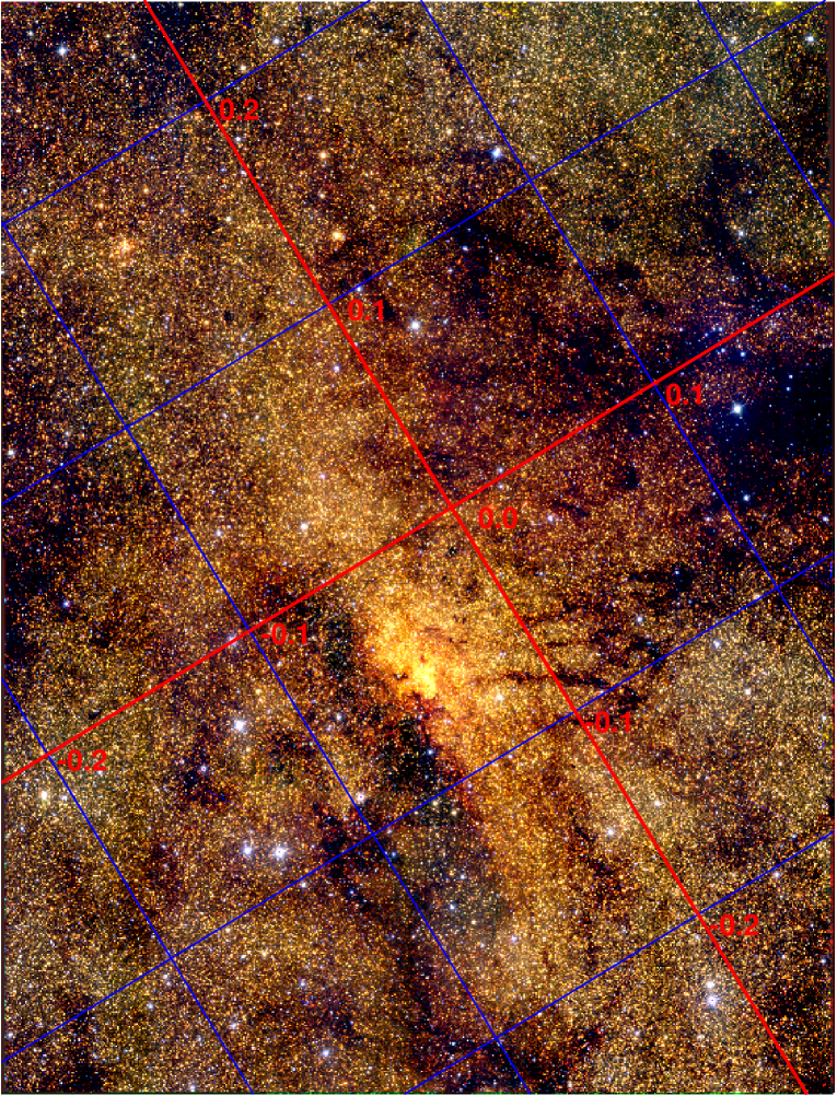
Figure 1: An $H$-band image (or an RGB composite image in the online journal) of the observed field. North in the equatorial system is up, and east is to the left. Solid (or red) lines indicate $l=0^{\circ}$ and $b=0^{\circ}$, while a grid with spacing of $0.1^{\circ}$ is shown with dashed lines (or blue ones). The covered area is about 20 arcmin by 30 arcmin.

Table 1: The observed fields. The central coordinates and the numbers of observations $N_{\mathrm{obs}}$ are indicated. We also list the number of sources ($N_{\mathrm{src}}$) and variables ($N_{\mathrm{var}}$) detected in each field as well as the total number in which we do not include duplicate detections in neighbouring fields.

Field	Centre (J2000.0)		Centre (Galactic)		$N_{\mathrm{obs}}$								$N_{\mathrm{src}}$	$N_{\mathrm{var}}$
	RA	Dec	$l(^{\circ})$	$b(^{\circ})$	2001	2002	2004	2005	2006	2007	2008	Total
1745-2900A	17:46:10.5	$-$28:53:47.8	$+0.0970$	$-0.0831$	1	1	0	47	42	2	1	94	9,266	128
1745-2900B	17:45:40.0	$-$28:53:47.8	$+0.0391$	$+0.0119$	0	1	0	47	41	2	1	92	6,797	132
1745-2900C	17:45:09.5	$-$28:53:47.8	$-0.0189$	$+0.1068$	1	1	0	45	40	2	1	90	6,041	89
1745-2900D	17:46:10.5	$-$29:00:28.0	$+0.0020$	$-0.1409$	1	1	0	46	42	2	1	93	8,692	104
1745-2900E	17:45:40.0	$-$29:00:28.0	$-0.0558$	$-0.0460$	1	1	0	45	41	2	1	91	8,451	225
1745-2900F	17:45:09.5	$-$29:00:28.0	$-0.1137$	$+0.0488$	1	1	0	43	41	2	1	89	8,185	151
1745-2900G	17:46:10.5	$-$29:07:07.8	$-0.0928$	$-0.1987$	1	1	0	41	41	2	1	87	9,576	101
1745-2900H	17:45:40.0	$-$29:07:07.8	$-0.1506$	$-0.1039$	1	1	0	43	41	2	1	89	7,399	123
1745-2900I	17:45:09.5	$-$29:07:07.8	$-0.2085$	$-0.0091$	0	1	0	43	36	2	1	83	8,747	122
1745-2940G	17:46:10.5	$-$28:47:07.9	$+0.1919$	$-0.0254$	1	1	1	41	38	2	1	85	8,885	174
1745-2940H	17:45:40.0	$-$28:47:07.9	$+0.1339$	$+0.0698$	1	1	1	40	39	2	1	85	9,237	130
1745-2940I	17:45:09.5	$-$28:47:07.9	$+0.0758$	$+0.1648$	1	1	1	15	40	2	0	60	8,636	80
Total													81,019	1,364

2.2 Pipeline reduction

The raw data were first processed by using the SIRIUS pipeline software (Yasushi Nakajima, private communication). A rough outline of the procedures is as follows. First, a dark image was subtracted from every raw image in order to eliminate the effect of dark current. We took ten frames with the shutter of the SIRIUS camera closed on every observing night. These were combined into one dark image. Then we corrected the pixel-to-pixel variation of sensitivity by dividing dark-subtracted images by a flat image. The flat image was produced from twilight-flat exposures. Several pairs of images with different sky levels were collected from twilight-flat images taken in sequence, and the differences between two images of the pairs were combined to produce a flat-field image after normalization. In order to subtract the background pattern of the images, we took exposures of a relatively sparse region with central coordinates 17:11:24.7, $-$27:27:20 (J2000.0). We took 10 dithered images of the blank field and combined them without adding any shifts to compensate for the dithering offsets. Thus we obtained a sky image without stellar signals but showing the background pattern of the images; this sky frame we subtracted from each flat-fielded image. The final step was to combine the 10 dithered images for a target field into a scientific image. Bright stars were selected in the sky-subtracted images, and the offsets among the images were calculated. The average of the images was taken after un-dithering them. The scientific image thus obtained is then free of spurious noise caused by bad pixels and cosmic ray events.

2.3 Photometry

Point-spread-function (PSF) fitting photometry was performed on the scientific images with the DAOPHOT package in IRAF. For each field one image taken under the best conditions (of weather and seeing) was selected from among the $N_{\mathrm{obs}}$ images for each filter as a reference frame. In order to standardize the magnitudes we compared the photometric result of the reference frame with the photometric catalogue by Nishiyama et al. (2006a). Their data were taken with the same instrument as ours. We used our own implementation of the Optimal Pattern Matching (OPM) algorithm (Tabur, 2007) to match stellar positions in our images and celestial coordinates given by Nishiyama et al. (2006a). The magnitudes we obtained are on the IRSF/SIRIUS natural system, whose zero-point calibration was based on a standard star in Persson et al. (1998).

We also performed PSF-fitting photometry using DAOPHOT for the remaining ($N_{\mathrm{obs}}-1$) images, and the results were compared with those from the reference frame. The comparisons were again made using the OPM algorithm. The positions are consistent among the images to within $\pm 0.1$ arcsec. We present examples of the magnitude comparisons in Fig. 2. The zero points of the magnitude scale for the ($N_{\mathrm{obs}}-1$) images were calibrated to fit with that of the reference based on 3-$\sigma$ clipped medians. The differences between magnitudes in the frames are distributed around zero for vast majority of stars, whilst the differences for variable stars follow their variations.

Figure 2: Examples of magnitude comparisons between the reference data ($\mathrm{MJD_{ref}}=53665.7594$ in this case) and repeated observations. These plots are for the 1745-2900A field and the MJDs of the target data are indicated on top of the panels.

2.4 Variability Detection

Using the procedures described in the preceding section, we obtained lists of the sources detected in $N_{\mathrm{obs}}$ images for each field and each filter. We expect that the faintest objects are detected only in some images due to variable conditions such as seeing. We included sources which were detected in $0.5N_{\mathrm{obs}}$ or more images in our catalogue. Using $N_{\mathrm{det}}$ to denote the number of detections of a given source, the condition can be written as $N_{\mathrm{det}}\geq 0.5N_{\mathrm{obs}}$. The number of detected sources, $N_{\mathrm{src}}$, is listed in Table 1 for each field. The total number for the 12 fields is also given. Fig. 3 shows histograms of $JHK_{\rm s}$ magnitudes and illustrates the detection limit. The shaded area is the histogram for sources with $N_{\mathrm{det}}\geq 0.8N_{\mathrm{obs}}$ while the outline is that for all the sources ($N_{\mathrm{det}}\geq 0.5N_{\mathrm{obs}}$). For a wide range of magnitudes, it is clear that the sources in our catalogue appear in almost all of the $N_{\mathrm{obs}}$ images. The numbers of detections start to decrease at the faint end. The detection limit for each image depends on the seeing and other weather conditions as well as the crowdedness, which varies considerably as seen in Fig. 1. We here define the typical limiting magnitude as that at which the number of sources with $N_{\mathrm{det}}\geq 0.8N_{\mathrm{obs}}$ becomes less than half of those with $N_{\mathrm{det}}\geq 0.5N_{\mathrm{obs}}$; $J=16.4$, $H=14.5$, and $K_{\mathrm{s}}=13.1$ mag. For sources fainter than these magnitudes it gets difficult to keep the detection ratios, $N_{\mathrm{det}}/N_{\mathrm{obs}}$, larger than 80 percent. The limits are indicated by the dotted lines in Fig. 3

We also found that the brightest sources are affected by deviations from linear response of the detectors. The deviation gets larger than 5 percent for objects brighter than $J=9.0$–$9.5$, $H=9.0$–$9.5$, or $K_{\mathrm{s}}=8.5$–$9.0$ mag. This limit is also dependent on seeing size and background brightness. In the following we do not consider magnitudes brighter than 9.5, 9.5, and 9.0 mag in $J$, $H$, and $K_{\mathrm{s}}$, respectively. We did not include measurements above the upper brightness limits in $N_{\mathrm{det}}$.

Figure 3: Histogram of $JHK_{\rm s}$ magnitudes of detected sources including non-variables. The shaded area is the histogram for sources with $N_{\mathrm{det}}\geq 0.8N_{\mathrm{obs}}$ while the outline indicates that for all the sources included in our source list ($N_{\mathrm{det}}\geq 0.5N_{\mathrm{obs}}$). The solid lines indicate the saturation limits while the dotted line do the detection limit (see text for their definitions).

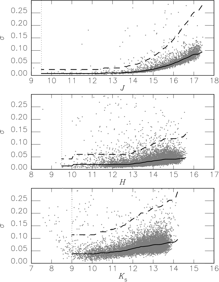
Figure 4: The standard deviation of $N_{\mathrm{det}}$ magnitudes is plotted against the mean magnitude for each object. The solid curves are the median errors at a given magnitude and the limits of non-variable stars are taken to be the dashed curves. The latter are shifted by a factor of three from the solid ones. See text for details.

Each source included in our list has magnitudes obtained for $N_{\mathrm{det}}$ images in each band, where $N_{\mathrm{det}}$ can be different for each of the $JHK_{\rm s}$ bands. We calculated the standard deviations (SDs) of the $N_{\mathrm{det}}$ magnitudes, which are plotted against the mean magnitudes in Fig. 4 for the case of the 1745-2900A field (as an example). As may be expected, the fainter sources tend to have the larger SDs. Assuming that the majority of the sources are not variable, at least to our photometric accuracy, their SDs arise from photometric errors. We estimated the error as a function of mean magnitude by taking the median of the SD at each magnitude. The median was calculated for every 0.1 mag interval, with a width of $\pm 0.2$ mag. This estimation was carried out from the faint to the bright end and we imposed the constraint that the error curve is a monotonically increasing function of magnitude, that is, $\sigma(m_{1})<\sigma(m_{2})$ if $m_{1}<m_{2}$ and $\sigma(m_{1})=\sigma(m_{2})$ otherwise. Examples of the error curves obtained are indicated by thick solid lines in Fig. 4. The vertical dotted lines indicate the limit brighter than which the magnitudes are affected by the deviation from linear response. The measurements over these limits are nevertheless plotted in Fig. 4 to illustrate such an effect. The stars affected have large SDs, as seen in the bottom ($K_{\mathrm{s}}$) panel, and are not considered further.

The SD values above which objects were taken to be candidate variables were obtained by multiplying the error curve by a factor of three and are plotted as the thick dashed lines in Fig. 4. For every candidate, we inspected the light curve and the appearance of its image by eye in order to determine whether the variation is real or spurious. The candidates excluded after inspection often lie near the edges of the images, causing their photometry to be affected. Some others are severely distorted by neighbouring bright star(s) that are saturated. At the same time, we searched for short-period variables with $0.1<P<60$ d among the candidate variables, which include Cepheids and eclipsing binaries. We found approximately 50 short-period variables. They are not included in this paper and will be reported in a forthcoming paper. The number of the remaining variables detected in each field, $N_{\mathrm{var}}$, is given in Table 1. When variables were found in two or more neighbouring fields near their edges, we confirmed that the light curves agreed and adopted only one entry for each variable. Thus 1364 long-period variables were selected for our catalogue.

3 Catalogue construction

In this section we discuss the estimation of periods, mean magnitudes, and their accuracies. We further carry out cross identifications with the surveys by G01 and Ramírez et al. (2008). The comparison with the G01 catalogue is, in some cases, useful for period estimation.

3.1 Comparison with Glass et al. (2001)

Miras listed in G01, also see Glass et al. (2002), were searched for in our catalogue. In order to adjust any systematic shifts in position between the two datasets, we added offsets to the positions in the G01 catalogue for the different G01 fields ($d_{\rm RA}$ and $d_{\rm Dec}$, given in Table 2). The application of these offsets led to better positional agreements. We found 348 matches with a tolerance of 3 arcsec. The standard deviations of the differences in Right Ascension (RA) and Declination (Dec) are approximately 0.5 arcsec after the offsets mentioned above.

G01 listed 12 duplicated detections of the Miras in their neighbouring fields in their table 3. In course of the cross identification, we found several more pairs of objects listed twice by G01. Their 2-18 and 3-7655 corresponds to 17453194-2857473 in our catalogue, while 4-6/19-23 to 17453003-2905100, 9-75/12-46 to 17461431-2854088, and 23-1198/24-2 to 17450596-2857483. We also found that 2-3 is identical to 16-24/17-1. The counterpart of 16-49 is 3-266, not 3-226 as listed in their paper. Additionally both 9-4 and 12-2 are close to one of the IRSF variables, 17461373-2855143, although they are slightly separated from each other. Their parameters are close to each other and consistent with the IRSF counterpart. We conclude that they are also the same object detected twice in neighbouring fields.

Among 56 G01 objects whose counterpart was not found, 39 are located outside our fields of view. Coordinates of the other 17 objects are within our survey area, but they are not detected as variable stars. We list those not identified in Table 3 with the suspected reasons for the failure. For example, the coordinate of 6-112 is rather close to a very bright star which is saturated in our images, while 6-112 is listed as rather faint. Its $Q$ flag given in the G01 catalogue is low and their photometry must have been affected by the saturated star. Both 12-799 and 12-1236 are separated from 17462073-2853253 by about 3 arcsec. Different parameters are given in G01 for these objects, and it is not clear which one corresponds to the IRSF variable. Their $Q$ flags are low. We did not consider the counterparts for these two G01 objects.

Table 2: The 25 fields in the G01 catalogue and the number of variables. $N_{\mathrm{G01}}$ – the number of objects reported in G01; $N_{\mathrm{mat}}$ – the number of the IRSF ones identified with those in G01; $d_{\rm RA}$ and $d_{\rm Dec}$ – offset between the coordinates in G01 and our catalogue. The total numbers after removing duplicate entries from neighbouring fields are listed in the last line.

Field	$N_{\mathrm{G01}}$	$N_{\mathrm{mat}}$	$d_{\mathrm{RA}}$ (arcsec)	$d_{\mathrm{Dec}}$ (arcsec)
GC1	14	14	$-0.57$	$1.01$
GC2	26	26	$-0.35$	$1.16$
GC3	35	32	$0.39$	$0.50$
GC4	13	13	$0.45$	$1.55$
GC5	10	7	$-0.30$	$1.14$
GC6	21	20	$-0.65$	$0.89$
GC7	15	14	$-0.54$	$0.74$
GC8	12	9	$-0.39$	$0.60$
GC9	23	23	$-0.99$	$0.97$
GC10	19	18	$-0.67$	$0.51$
GC11	11	7	$2.64$	$0.83$
GC12	22	15	$-0.31$	$0.07$
GC13	20	18	$-0.34$	$0.71$
GC14	18	16	$-0.29$	$0.93$
GC15	8	5	$0.13$	$0.78$
GC16	26	25	$-0.52$	$0.69$
GC17	17	16	$-0.16$	$0.81$
GC18	7	7	$0.13$	$0.79$
GC19	21	20	$-0.09$	$0.93$
GC20	19	11	$-0.17$	$0.70$
GC21	10	4	$-0.16$	$0.88$
GC22	23	20	$-0.20$	$0.92$
GC23	21	16	$-0.34$	$0.57$
GC24	5	4	$0.13$	$1.25$
GC25	6	5	$-0.26$	$0.94$
Total∗	405	348

^∗Duplicate detections in neighbouring fields are not counted.

Table 3: G01 variables whose counterparts were not found in our survey. Superscripts ($a$–$d$) indicate our suggested explanations.

Field	Unmatched objects
3	2389d, 2832b, 2834b
5	59a, 164a, 2856a
6	112d
7	361d
8	5a, 31a, 97b
10	60b
11	23a, 27a, 2449a, 4503b
12	2d, 6a, 11a, 136a, 228a, 799d, 1236d
13	30a, 73a
14	150a, 463a
15	5a, 10a, 26a
16	2993d
17	118c
19	685d
20	11a, 22a, 46a, 70a, 99a, 116a, 133b, 522c
21	6a, 8a, 17a, 38a, 185a, 5719a
22	31d, 60a, 100a
23	5a, 15c, 42a, 50a, 114a
24	29a
25	7a

^a The object is located out of our survey area. ^b A probable counterpart exists in our image, but we did not detect variability. ^c Two or more stars are visible with approximately the expected brightness, but we did not detect any corresponding variation. ^d We found no clear counterpart at around the given coordinate.

We plotted a histogram of $K/K_{\mathrm{s}}$ mean magnitudes which appear in both the G01 catalogue and ours in Fig. 5. We used only good estimates of $K_{\mathrm{s}}$ magnitudes for which ${\rm Mflag}=0$ is given (see section 3.3). Although we cannot directly compare the magnitudes obtained with different filters, $K$ and $K_{\mathrm{s}}$, their difference is not expected to be large. It is obvious that many bright sources are saturated in our data and that many fainter ones were not detected in G01. With our better image quality, our detection limit is deeper and we also discovered many new variables which are brighter than the faintest G01 objects ($K\sim 12$), as well as fainter variables. Whilst many G01 variables were saturated in our $K_{\mathrm{s}}$-band images, a large fraction of them were detected in the $J$- and/or $H$-bands. There are 348 matches between the two catalogues and none of these were saturated in our $J$-band images. It should also be mentioned that saturation was not the reason for the 56 unsuccessful matches (see Table 3).

Figure 5: Histogram of $K_{\mathrm{s}}$ magnitudes which appear in our catalogue (the thick outline) and $K$ magnitudes of the G01 variables (hatched region)

3.2 Estimation of periods

We used both our own data and the G01 catalogue in order to estimate the periods of the detected variables. First we carried out a period search of our monitoring data using the least-squares method to fit sinusoidal curves. We searched for periods between 100 and 800 d fitting sinusoidal curves with minimum residuals. Then we examined the light curve folded with the obtained period by eye. We confirmed the periods for 483 variable stars. The periods obtained by us are written as $P_{\mathrm{IRSF}}$.

There are 246 sources for which G01 obtained periods, $P_{\mathrm{G01}}$, among the variables that have $P_{\mathrm{IRSF}}$ values. We have plotted $\log(P_{\mathrm{G01}}/P_{\mathrm{IRSF}})$ values against $\log(P_{\mathrm{IRSF}})$ in Fig. 6. The periods agree with each other in most cases. The standard deviation of $\log(P_{\mathrm{G01}}/P_{\mathrm{IRSF}})$ around zero is 0.025, where we have included those within $\pm 0.1$ dex. This indicates that the accuracies of the periods estimated by us and by G01 are within 0.025 dex in most cases. We conclude that $P_{\mathrm{G01}}$ and $P_{\mathrm{IRSF}}$ are consistent with each other when their difference is less than 0.075 dex; this level is indicated by the horizontal dashed lines in Fig. 6. When the values are consistent we take the period as $P_{\mathrm{IRSF}}$ in our catalogue. For the 25 objects where $P_{\mathrm{G01}}$ is not consistent with $P_{\mathrm{IRSF}}$ we also use $P_{\mathrm{IRSF}}$. For the objects with counterparts in G01, we can combine their photometry with ours to estimate the period. We fitted sinusoidal light curves for both $K$-band (G01) and $K_{\mathrm{s}}$-band (ours) photometry; means and amplitudes are independently obtained for two datasets allowing differences in $K$- and $K_{\mathrm{s}}$-band, but common periods and dates of maxima are used for the fitting. These procedures allow us to carry out better period estimations using the photometry with a long time coverage of 1994–2008. We confirmed that thus obtained periods agree well with $P_{\mathrm{IRSF}}$ to within $\pm 0.01$ dex, and we replaced the $P_{\mathrm{IRSF}}$ whenever possible.

There are 96 variables with $P_{\mathrm{G01}}$ among the variables whose periods were not obtained by us. For 66 of them, we have confirmed that $P_{\mathrm{G01}}$ can reasonably be used to explain the variations we detected. We have adopted those $P_{\mathrm{G01}}$ in our catalogue. However, $P_{\mathrm{G01}}$ does not fit the light curves for the remaining 30 variables. We use ${\rm Pflag}$ as defined in Table 4 to indicate the status of the periods. The numbers of variables with each ${\rm Pflag}$ are also given in Table 4. In summary, we obtained periods for 549 variables (${\rm Pflag}=0$ to 3). Light curves folded with the obtained periods are included in the online material. Fig. 7 shows examples of the light curves for the twenty-five cases having the shortest periods.

Figure 6: Comparison of $P_{\mathrm{IRSF}}$ and $P_{\mathrm{G01}}$. The $\log~{}(P_{\mathrm{G01}}/P_{\mathrm{IRSF}})$ values are plotted against $\log~{}(P_{\mathrm{IRSF}})$ whenever possible. The dashed lines indicate the range of $\pm 0.075$ dex within which we conclude $P_{\mathrm{IRSF}}$ and $P_{\mathrm{G01}}$ agree with each other.

Table 4: Definition of ${\rm Pflag}$. Number of variables with each ${\rm Pflag}$ is also given.

${\rm Pflag}$	$N_{\mathrm{var}}$	Note
0	221	$P_{\mathrm{G01}}$ and $P_{\mathrm{IRSF}}$ agree with each other to within 0.075 dex. We adopt $P_{\mathrm{IRSF}}$.
1	25	$P_{\mathrm{G01}}$ and $P_{\mathrm{IRSF}}$ disagree and we adopt $P_{\mathrm{IRSF}}$.
2	237	$P_{\mathrm{G01}}$ is not given and we adopt $P_{\mathrm{IRSF}}$.
3	66	$P_{\mathrm{G01}}$ fit our light curve but $P_{\mathrm{IRSF}}$ is not properly obtained. We adopt $P_{\mathrm{G01}}$.
4	30	$P_{\mathrm{G01}}$ does not fit the IRSF light curve. No periodicity is found.
5	785	$P_{\mathrm{G01}}$ is not given and no clear periodicity is found with the IRSF data.

Figure 7: Examples of periodic light curves are plotted for 25 Miras with the shortest periods. In each panel we list ID, period (d), and name of filter used for the plot. Plots for all of those with given period are available as online material.

3.3 Estimation of mean magnitudes

In this paper, for simplicity, we define our mean magnitude as the intensity mean of the maximum and minimum of our measurements of a given star. We can apply this definition, unlike Fourier means, regardless of whether or not the light curve is periodic. Another possible definition is an intensity mean of all the measurements, but this can be affected by uneven sampling.

In order to trust any photometric distance scale, it is important to obtain magnitudes for both targets and calibrators in the same manner. In the case of the PLR for pulsating stars, the definition of mean magnitude can have a significant effect. For example, intensity means differ from magnitude means. In our case, we will estimate mean magnitudes in the same manner as Ita et al. (2004b, hereafter I04) because we will use their catalogue to calibrate our PLR (see section 5.1). I04 combined images at ten arbitrary epochs before carrying out photometry, so that their magnitudes correspond to intensity means of ten points. Because we have observations at more epochs, approximately 90 in most cases, we should be able to get better estimates of mean magnitudes. Nevertheless, it is necessary to be careful about any systematic difference between our means and those in I04.

We have performed Monte-Carlo simulations to assess the uncertainties of the ten-epoch means and their systematic difference from ours, if any. First, we randomly produced ten values between 0 and 1 as test phases, and for each of them we obtained a magnitude from an interpolation between the closest points on both sides of our folded light curve. Then, we took an intensity mean of the magnitudes at the selected ten phases, which gives us a simulated value for a ten-epoch mean. We repeated these procedures ten thousand times for each light curve to get simulated magnitudes, $m_{\mathrm{sim}}$. Then we examined how the ten-epoch intensity mean varies, depending on the randomly selected phases. We illustrate three examples of the simulations in Fig. 8. The histograms indicate how the simulated means, $H_{\mathrm{sim}}$, are distributed around the means of maximum and minimum, which are indicated by the vertical dashed lines. The dispersions $\sigma_{\mathrm{sim}}$ of the histograms suggest that a ten-epoch mean may have a significant uncertainty as large as $\pm 0.1$ mag (e.g. the middle panel of Fig. 8). Furthermore, the means of the simulated magnitudes $\langle m_{\mathrm{sim}}\rangle$ do not always agree with the vertical lines. Such differences depend on the shapes of the light curves.

Figure 8: Three examples of Monte-Carlo simulations of mean magnitudes from ten-epoch data are shown. For each $H$-band light curve displayed in the small frame, intensity means were repeatedly calculated for randomly defined groups of ten epochs. The means obtained are plotted as a histogram, while the thick dashed line indicates the intensity mean of maximum and minimum, as listed in the catalogue.

We now examine whether the difference between I04 and our results introduces a systematic offset or not. We consider only light curves which have good coverage in phase for the Monte-Carlo simulations. We also exclude light curves whose periods are not confirmed with our data (i.e. ${\rm Pflag}$ in section 3.2 should be 0, 1, or 2). There are 48 ($J$), 84 ($H$), and 85 ($K_{\mathrm{s}}$) such light curves without any gap larger than 0.2 in phase among those with $P=100$–$350$ d. We calculate differences between the means from our observation and those from the simulations, i.e. $m-\langle m_{\mathrm{sim}}\rangle$, which are plotted against amplitudes in Fig. 9. The uncertainties $\sigma_{\mathrm{sim}}$ of a ten-epoch mean inferred from the simulations are indicated by error bars. One finds that both $|m-\langle m_{\mathrm{sim}}\rangle|$ and $\sigma_{\mathrm{sim}}$ tend to be large for light curves with large amplitude. The amplitudes of the examples presented in Fig. 8 are moderate among our sample. The weighted mean of the differences is close to zero. This suggests that the difference between our means and those in I04 is small, within $\pm 0.01$ mag or less.

Figure 9: Expected differences between means obtained from observation, $m$, and those from the Monte-Carlo simulations, $\langle m_{\mathrm{sim}}\rangle$. The size of an error bar indicates the uncertainty in $\langle m_{\mathrm{sim}}\rangle$.

We calculate the mean magnitudes, defined as intensity means of maximum and minimum, in $JHK_{\rm s}$ whenever possible. However, we did not always detect variables in all the three bands. Some variables are detected in $H$ and $K_{\mathrm{s}}$ but are too faint in $J$, while some others are detected in $J$ and $H$ but are too bright and saturated in $K_{\mathrm{s}}$-band. We define the ${\rm Mflag}$ as described in Table 5 in order to give an idea of the quality of the magnitude or a reason why there was no detection in a particular band. In some cases, the number of detections is enough to include the object in our list, i.e. $N_{\mathrm{det}}\geq 0.5N_{\mathrm{obs}}$, but a few measurements are missing at around maximum or minimum for instrumental reasons. We checked light curves for which we failed to get one or more points. The phases of the failures were indicated in the plots and we examined whether the unavailable points may have had a significant effect on the mean magnitudes, based on the shapes of the light curves in a given filter and in other filter(s) when available. Then we determined whether the light curves are affected (${\rm Mflag}=4$–$6$) or not (${\rm Mflag}=0$). The ${\rm Mflag}$ for each variable has three digits between 0 and 7, each of which denotes the state of (un)available magnitudes in the order of $J$, $H$, and $K_{\mathrm{s}}$.

Table 5: Definition of ${\rm Mflag}$. The number of variables with each ${\rm Mflag}$ is also given for $J$, $H$, and $K_{\mathrm{s}}$ magnitudes respectively.

${\rm Mflag}$	$N_{J}$	$N_{H}$	$N_{K_{\mathrm{s}}}$	Note
0	361	990	936	The magnitude was obtained without any clear problems.
1	9	0	2	We did not obtain the magnitude because the object often falls out of the field of view.
2	0	18	222	We did not obtain the magnitude because the object is too bright.
3	833	178	4	We did not obtain the magnitude because the object is too faint.
4	15	35	21	We obtained the mean magnitude, but it is affected by its location around the edge of the images.
5	2	19	116	We obtained the mean magnitude, but it is affected by saturation or deviation from linear response.
6	144	124	63	We obtained the mean magnitude, but it is affected by the fact that the object was not detected in some cases because of its faintness.

3.4 Comparison with Ramírez et al. (2008)

Ramírez et al. (2008) compiled a catalogue of 1,065,565 sources in the $2.0^{\circ}\times 1.4^{\circ}$ region around the GC based on their Spitzer/IRAC survey. About 60,000 objects lie within the field we observed. They obtained magnitudes in four wave-passbands, i.e. ${[3.6]},{[4.5]},{[5.8]}$, and ${[8.0]}$, so that we can investigate features of our objects at longer wavelengths by making use of their results. We identified 1,233 counterparts in their catalogue with a tolerance of 0.5 arcsec. The coordinates in the two catalogues agree very well, with standard deviations of 0.13 arcsec in RA and Dec.

3.5 The catalogue

We present the first ten lines of our catalogue in Table 6, as an example. The entire list is available in machine-readable form in the online version of this article. We include ID, mean magnitudes ($JHK_{\rm s}$), peak-to-peak amplitudes ($\Delta J,\Delta H,\Delta K_{\mathrm{s}}$), and ${\rm Mflag}$ (see Table 5). The magnitudes and the amplitudes are listed as 99.99 and 0.00 respectively when we did not detect the object in a given band. We also list the IDs of the sources in G01 and Ramírez et al. (2008) whenever counterparts were found. For those with period available, $P$ and ${\rm Pflag}$ (see Table 4) are also indicated. We also present a list of photometric measurements. The $JHK_{\rm s}$ magnitudes obtained for all the catalogued variables are listed in one text file and each line includes the ID number, the modified Julian date (MJD), and the $JHK_{\rm s}$ for a given star. Table 7 shows the first ten lines as a sample.

Table 6: Catalogue of variable stars. After the numbering ID between 1 and 1364, the ID from RA and Dec (J2000.0) follows. $JHK_{\rm s}$ mean magnitudes and peak-to-peak amplitudes are listed together with ${\rm Mflag}$ (section 3.3). When the magnitudes and the amplitudes are unavailable, we put 99.99 and 0.00, respectively. Counterparts of Ramírez et al. (2008) and Glass et al. (2001) are indicated whenever identified. Also listed are periods (000 when not available) and Pflag(section 3.2). This is the first ten lines of the full catalogue which will be available in the online version.

No.	ID	Mean magnitude			Amplitude			Mflag	Counterpart		Period	Pflag
		$J$	$H$	$K_{\mathrm{s}}$	$\Delta J$	$\Delta H$	$\Delta K_{\mathrm{s}}$		R08	G01
0001	17445379-2857241	99.99	11.71	9.51	0.00	0.34	0.38	100	0401463	–	000	5
0002	17445418-2906303	99.99	12.50	9.71	0.00	0.94	0.71	300	0402528	22-166	339	0
0003	17445435-2857415	99.99	11.39	9.15	0.00	0.88	0.33	105	0402897	–	424	2
0004	17445435-2904563	12.76	10.05	99.99	0.87	1.12	0.00	002	0402921	22-14	280	3
0005	17445442-2856527	99.99	12.91	10.64	0.00	0.30	0.22	300	0403085	–	000	5
0006	17445452-2856168	99.99	13.35	11.09	0.00	0.62	0.44	300	0403313	–	000	5
0007	17445460-2852042	99.99	13.87	10.64	0.00	0.64	1.12	360	0403552	–	000	5
0008	17445463-2903587	99.99	13.50	10.13	0.00	1.68	1.48	360	0403617	–	457	2
0009	17445482-2903208	14.12	10.82	99.99	0.53	0.36	0.00	002	0404128	–	000	5
0010	17445482-2905486	16.13	11.87	9.46	0.58	0.54	0.60	000	0404117	–	313	2

Table 7: The first 10 lines of the released table of light variation. This is a sample of the full version (116887 lines), which will be available in the online version of this journal.

No.	MJD	$J$	$H$	$K_{\mathrm{s}}$
0001	52079.9757	99.99	11.62	9.52
0001	52343.1326	99.99	11.62	9.68
0001	53482.0590	99.99	11.76	9.54
0001	53537.1116	99.99	11.79	9.55
0001	53540.8221	99.99	11.83	9.58
0001	53545.8849	99.99	11.84	9.64
0001	53545.9694	99.99	11.85	9.57
0001	53548.8259	99.99	11.81	9.54
0001	53548.9591	99.99	11.84	9.56
0001	53549.8893	99.99	11.84	9.62

4 Properties of catalogued variables

4.1 Magnitude and photometric flag

Among the 1364 catalogued variables, we detected 522 variables in $J$, with 1168 in $H$ and 1136 in $K_{\mathrm{s}}$. If we restrict ourselves to those with ${\rm Mflag}$ = 0, the numbers of variables are 361, 990, and 936 in $J$, $H$, and $K_{\mathrm{s}}$ respectively (Table 5). Table 8 indicates the number and percentage for each combination of bands in which variables are detected. For example, we detected 303 variables in all of the $JHK_{\rm s}$ filters while 178 were detected only in $K_{\mathrm{s}}$. If we consider only magnitudes with ${\rm Mflag}$ = 0, the above numbers reduce to 119 and 121, respectively. Approximately 70 percent of the catalogued variables have both $H$ and $K_{\mathrm{s}}$ magnitudes (22.2 percent with $JHK_{\rm s}$ and 48.0 percent with $HK_{\mathrm{s}}$).

Table 8: Combinations of bands in which we detected variables. The number and percentage are given for each combination. The values in parentheses count only variables with photometry flags of 0 for the given filters.

Band combination	Number		Percentage (%)
$J+H+K_{\mathrm{s}}$	303	(119)	22.2	(8.7)
$\hskip 8.53581pt+H+K_{\mathrm{s}}$	655	(485)	48.0	(35.6)
$J+\hskip 8.53581pt+K_{\mathrm{s}}$	0	(0)	0.0	(0.0)
$J+H+\hskip 8.53581pt$	201	(152)	14.7	(11.1)
$J\hskip 34.1433pt$	18	(14)	1.3	(1.0)
$\hskip 17.07164ptH\hskip 17.07164pt$	9	(7)	0.7	(0.5)
$\hskip 34.1433ptK_{\mathrm{s}}$	178	(121)	13.0	(8.9)
Total	1364		100.0

We have plotted histograms of $J$, $H$, $K_{\mathrm{s}}$, and $H-K_{\mathrm{s}}$ in Fig. 10. Only magnitudes with ${\rm Mflag}=0$ are considered. The hatched regions correspond to the histograms for the variables whose $JHK_{\rm s}$ magnitudes are all available. Those with $JHK_{\rm s}$ magnitudes occupy different ranges in the three panels. For $J$- and $H$-band magnitudes, the brightest objects tend to lack $K_{\mathrm{s}}$-band magnitudes (see the regions of $J<14$ and $H<11$). This is because the corresponding objects are too bright in $K_{\mathrm{s}}$. In contrast, $J$-band magnitudes are not available for a large number of objects which are faint in $H$ and $K_{\mathrm{s}}$ ($H>12.5$ and $K_{\mathrm{s}}>10.5$). This is because these objects are too faint in $J$, predominantly because they suffer from strong interstellar extinction. The bottom panel shows that only relatively blue variables have all the $JHK_{\rm s}$ magnitudes, supporting the conclusions above.

Figure 10: Histograms of obtained magnitudes, $J$, $H$ and $K_{\mathrm{s}}$ from top to bottom and also that of the $H-K_{\mathrm{s}}$ colour. Those for the objects with three-band magnitudes are shaded.

4.2 Colour-magnitude and colour-colour diagram

In Fig. 11, we present colour-magnitude diagrams for our catalogued variables (black points for those with ${\rm Mflag}=0$ and black crosses for those with ${\rm Mflag}=4$–$6$) and non-variables (grey dots). The arrows indicate the reddening vector directions, with lengths corresponding to $A_{K_{\mathrm{s}}}=1$ mag. It is apparent that the objects with strong extinction are often fainter than the detection limit, especially in the $J$-band.

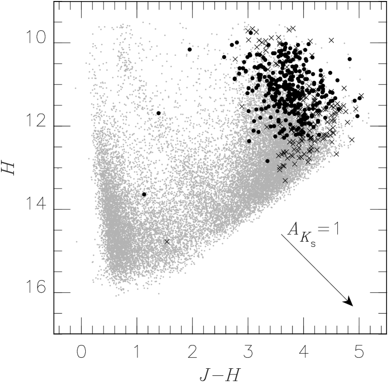
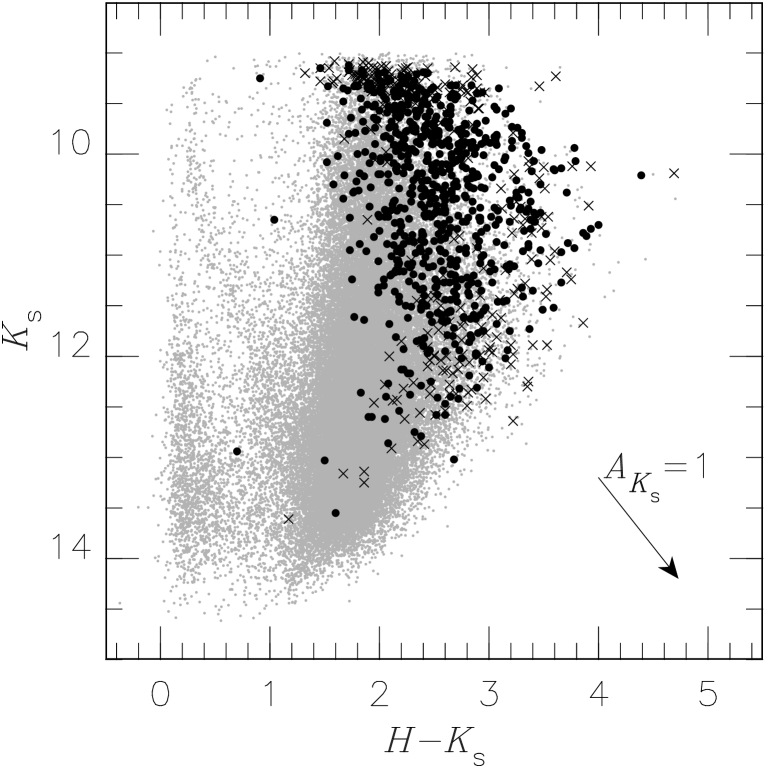
Figure 11: Colour-magnitude diagrams, $(J-H)$-$H$ in the top panel and $(H-K_{\mathrm{s}})$-$K_{\mathrm{s}}$ in the bottom. The black points show the distribution of the catalogued variables with ${\rm Mflag}=0$ while the black crosses include those with ${\rm Mflag}=4$–$6$. Grey dots show all the detected non-variable sources. The arrow indicates the reddening vector corresponding to $A_{K_{\mathrm{s}}}=1$ mag.

We also plot the colour-colour diagram in Fig. 12. Due to large and variable extinction, the distribution of sources is elongated along the direction of the reddening vector. There is a group of stars which scatter towards the right side of the main diagonal sequence. We inspected these stars on the images and found that tiny displacements of centroid are recognizable among the $JHK_{\rm s}$ images for at least some of them. In Fig. 13, we plot histograms of the differences between positions, both RA and Dec, obtained in $J$ and $K_{\mathrm{s}}$ images for individual sources. The panels (a) and (b) include the objects belonging to the main group and the distributions resemble Gaussian functions centred on zero as expected. On the other hand, the panels (c) and (d) include objects with peculiar colours, i.e. $J-H<1.767(H-K_{\mathrm{s}})-1.0$, and show totally different distributions from those in (a) and (b). There is no sharp peak at zero and the differences distribute rather uniformly. This clearly suggests that different stars having almost the same positions were incorrectly combined to produce sources with peculiar colours. In other words, different stars may contribute to the fluxes we measured in the images in different filters: a bluer star to the $J$-band flux and a redder star to $K_{\mathrm{s}}$-band. If we combine the flux of a foreground star on the main sequence and that of a reddened giant, for example, the combined source will be located on the right side of the main distribution in Fig. 12. The objects with $J-H<1.767(H-K_{\mathrm{s}})-1.0$ constitute not more than 3 percent of the number of sources with all three $JHK_{\rm s}$ magnitudes, so that they hardly affect any of our results.

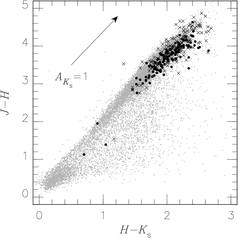
Figure 12: Colour-colour diagram, $(H-K_{\mathrm{s}})$ – $(J-H)$. Symbols are the same as in Fig. 11. The arrow indicates the reddening vector corresponding to $A_{K_{\mathrm{s}}}=1$ mag.

Figure 13: Histograms of the difference between positions in $J$ and $K_{\mathrm{s}}$ images. The upper panels (a) and (b) are for objects with normal locations in the colour-colour diagram, while the lower panels (c) and (d) are for objects with peculiar locations, i.e.  $J-H<1.767(H-K_{\mathrm{s}})-1$.

4.3 Period distribution

We have plotted period histograms for the variables in our catalogue and also in a few others (Fig. 14). Compared with the sample in G01 (the shaded area) in the top panel, we have added significantly more variables with periods (see the thick line). The other panels show the histograms for the variables in Whitelock, Feast & Catchpole (1991, middle) and in M05 (bottom). Their objects are located away from the GC. The sample in Whitelock et al. (1991) was selected from the IRAS point-source catalogue, while M05 investigated variables found in the OGLE variability catalogue (Woźniak et al., 2002). Because of the selection bias caused by the different wavelengths used in the surveys, the period distributions in these two early studies are different from each other as discussed in M05. The former has variables with $P>600$ d, while the latter has a more significant tail towards the short period end. In contrast, the histogram for our catalogue includes both the long-period variables and the short-period tail. It is suggested that our catalogue contains a more comprehensive sample of Miras than previous ones.

Figure 14: Histograms of periods. In the top panel, the thick line shows the histogram of the periods adopted in our catalogue, while the shaded area indicates that of $P_{\mathrm{G01}}$ for the G01 variables with IRSF counterpart. In the middle and bottom panels shown are the period distributions reported in Whitelock et al. (1991) and M05 respectively.

4.4 Amplitude distribution

Fig. 15 shows histograms of peak-to-peak amplitudes in $JHK_{\rm s}$. The hatched region corresponds to the variables with periods (191 in $J$, 432 in $H$ and 319 in $K_{\mathrm{s}}$), while the outline includes all the variables with ${\rm Mflag}=0$ detected in each filter. The histogram of $\Delta J$ shows separated peaks: one for small-amplitude variables ($\Delta J<0.5$) and the other(s) for large-amplitude variables. Such a distribution is also seen in the histogram of optical amplitudes (e.g. see fig. 4 and 6 in Glass & Lloyd Evans 2003). Many of the large-amplitude variables have been found to be periodic as expected for Miras, whilst we failed to obtain periods for many of the small-amplitude ones. The separation gets less conspicuous as the wavelength increases. The hatched region in the $\Delta K_{\mathrm{s}}$ panel resembles the distribution for Miras reported by Glass et al. (1995; see their fig. 3).

It is traditional to separate the Miras from the other long-period variables such as semi-regulars by their large visible amplitudes, i.e.  $\Delta V\geq 2.5$ mag. As we will see in section 5.1, we select periodic variables with $\Delta I>1$ mag among the LMC variables reported in I04 to calibrate the PLR. However, we do not have $V$- or $I$-band amplitudes for our objects. Most Miras have amplitudes larger than 0.4 mag in $K$ (e.g. see Whitelock, Marang & Feast, 2000), but the threshold in the near-IR amplitudes is not well established. It is even unclear if one can pick up the same group of Miras by using observables at different wavelengths. There are some periodic variables with relatively small amplitude. For example, 17451726-2844420 ($P=133$) and 17462476-2902241 ($P=177$) have rather small amplitudes ($\Delta J<0.3$ mag), but their light curves show reasonably periodic variations (Fig. 7). These objects may be SRa type, which can be as periodic as Miras but are distinguished by having relatively small amplitudes. However, some recent studies have raised questions on the distinction between the Miras and at least some of the semi-regulars. Lebzelter, Schultheis & Melchior (2002), for example, showed that a sizeable number of small-amplitude variables are as regular as Miras.

The most important requirement in our selection is that our distance indicators follow the PLR of Miras. There are several sequences in the well-known period-luminosity diagram of pulsating red giants (Wood et al. 1998; Ita et al. 2004a). Nevertheless, it is known that Miras if properly chosen are exclusively found on the sequence C, which makes them valuable distance indicators. Unfortunately, it is currently impossible to tell which sequence a given small-amplitude variable is located on as Feast (2004) pointed out. Some small-amplitude variables coexist with Miras on the sequence C. We here consider a periodic variable to be a Mira if its $\Delta J$, $\Delta H$, or $\Delta K_{\mathrm{s}}$, whichever may be available, is not less than 0.4 mag. Among our objects with periods, the number of such small-amplitude variables excluded is not large, about 10 percent. As will be discussed in section 5.2.1, at least some of the small-amplitude variables seem to be on a different sequence from that of Miras in the P-L diagram.

Figure 15: Histogram of amplitudes: $\Delta J$, $\Delta H$ and $\Delta K_{\mathrm{s}}$ from the top panel to the bottom. The outline includes all the variables, while the shaded area indicates those with period.

Fig. 16 shows $K_{\mathrm{s}}$-band amplitude plotted against period. One finds that the amplitudes do not exceed 1.5 mag for those with $P=100$–$350$ d, which we will use as distance indicators. This property does not change in the cases of $\Delta J$ and $\Delta H$.

Figure 16: Amplitudes in the $K_{\mathrm{s}}$-band plotted against periods.

4.5 Mid-IR properties

Using the counterparts identified in the catalogue by Ramírez et al. (2008), we can study the mid-IR properties of our variables. We have plotted $K_{\mathrm{s}}-{[8.0]}$ colour against period and amplitude for 282 Miras with ${\rm Mflag}=0$ in $K_{\mathrm{s}}$. In the top panel of Fig. 17, the mid-IR colour becomes large at the long-period end, $P>350$ d, similar to the amplitude trend illustrated in Fig. 16. The lower panel of Fig. 17 shows that the variables with large enhancement in $K_{\mathrm{s}}-{[8.0]}$ are, in fact, associated with large amplitudes. We also examined similar plots using ${[3.6]},{[4.5]}$ and ${[5.8]}$ magnitudes instead of ${[8.0]}$, and found similar trends. A large excess in the mid IR is expected for a thick circumstellar dust shell produced through mass-loss. This behaviour is well known from early observations (e.g. Whitelock et al. 1994). Detailed study of the mid-IR properties and the mass-loss process is outside the scope of this paper. Please note that no correction has been made for interstellar extinction and also that the mid-IR magnitudes from Ramírez et al. (2008) were obtained from a single-epoch survey made with Spitzer Space telescope.

Figure 17: The $K_{\mathrm{s}}-{[8.0]}$ colours are plotted against the periods (top) and the amplitudes (bottom) for periodic variables.

5 Distance and Reddening

5.1 Relation from the LMC

In this paper we make use of the PLR for Miras in the LMC in order to make distance estimations. I04 published a near-IR catalogue of LMC variables which were detected in the OGLE-II survey by Udalski, Kubiak & Szymański (1997). We select 134 Miras under the following criteria,

• $\Delta I>1$,

• $J-K_{\mathrm{s}}<1.4$,

• $K_{\mathrm{s}}<13$,

• $P\leq 350$,

as calibrators. The colour criterion is used to exclude carbon-rich stars. Miras in the Galactic bulge are predominantly oxygen-rich (see Schultheis, Glass & Cioni, 2004, for example). The last criterion is used to exclude objects with thick circumstellar dust and hot-bottom-burning stars (Whitelock et al. 2003; Glass & Lloyd Evans 2003). The near-IR observations for the I04 catalogue also made use of IRSF/SIRIUS. Although I04 converted their magnitudes into the system of the Las Campanas Observatory (LCO), we have converted them back into the natural system of the IRSF/SIRIUS based on the transformation they used. Fig. 18 plots the $JHK_{\rm s}$ magnitudes against periods. The period distribution of the LMC calibrators is rather uniform except the longest period range ($\log P>2.44$). In this range more carbon-rich variables are found in the LMC than oxygen-rich ones (Groenewegen, 2004). This situation is different from that of the Galactic bulge. Nevertheless, the effect of the period distribution in determining the PLR is small if any. There has been no report to offer evidence of a change in the slope of the PLR.

The PLR can be determined to be:

$$M_{J}=-2.875(\log P-2.3)-5.798,$$ (1)

$$M_{H}=-3.186(\log P-2.3)-6.508,$$ (2)

$$M_{K_{\mathrm{s}}}=-3.555(\log P-2.3)-6.883,$$ (3)

with residual standard deviations of 0.19, 0.19 and 0.17 mag, respectively. The distance of the LMC is assumed to be 18.45 mag (see section 5.3 for its uncertainty) and extinction corrections of $A_{J}=0.06$, $A_{H}=0.03$ and $A_{K_{\mathrm{s}}}=0.02$ have been applied. The residual scatter is least in $K_{\mathrm{s}}$, but the differences are small. This indicates that the PLR in $J$ and $H$ can also be useful for distance estimation. More importantly, one can estimate the amount of interstellar extinction together with the distance by using the PLR in two or more wavebands. The residual scatter is slightly larger than that in Feast et al. (1989) for the $\log P$-$K_{\mathrm{s}}$ relation while those around the PLRs in $J$ and $H$ are similar. The relatively large scatter is presumably because the magnitudes in I04 were obtained as intensity means based on ten-epoch monitorings. The simulation presented in section 3.3 suggests that the ten-epoch mean can have an uncertainty of $\pm 0.1$ mag compared to a well determined value. One can expect that the scatter reduces to that reported in Feast et al. (1989) after mean magnitudes are properly obtained.

Figure 18: Period-luminosity relation for Miras in the LMC, plotted for 134 O-rich Miras selected from the catalogue of I04 (see text for the selection criteria).

It is necessary to call attention to possible differences between Miras in the LMC and those around the GC. It is suspected that the PLR of Miras may be dependent on stellar parameters such as metallicity. Readers are referred to Whitelock et al. (2008) for a review of the PLRs in different environments. On the other hand, a difference in photometric systems can also have a large effect. Fig. 19 plots period-colour relation (PCR) for the Miras in the LMC (Feast et al. 1989; I04) and those in the Galactic bulge (Glass et al. 1995; M05). For the relation of Glass et al. (1995), we calculated the PCR by using the samples with period shorter than 350 d after two objects with extreme colours were omitted. Lines are drawn for a period range of samples in each paper; the shortest period in Glass et al. (1995) is around $\log P=2.2$, while there are several objects with period close to 100 d in I04 and M05. Feast et al. (1989) and Glass et al. (1995) used the Mk III photometer attached to the 1.9-m telescope at SAAO Sutherland to observe the Miras in the LMC and those in the Galactic bulge towards the Sgr I window respectively. Observations by I04 were conducted by using the IRSF/SIRIUS also at Sutherland, while M05 used $JHK_{\rm s}$ magnitudes taken from the 2MASS point-source catalogue (Skrutskie et al., 2006). Although transformations between these systems are available for normal types of stars, it is highly uncertain whether they are applicable to Miras which have strong absorption due to H₂O and other molecules. Based on Fig. 19, it is difficult to discuss any population effect that may exist between the Miras in the two populations. Especially in the $\log P$-$(J-H)_{0}$ diagram, the difference between the instruments seems to have a larger effect than any possible population differences. We will therefore use the PLR, eqs. 1–3, obtained from the observations by I04. The possible population effect will be discussed again in section 5.3.

Figure 19: Period-colour relations for Miras obtained in earlier papers. Line styles and widths for different samples are indicated at the top: F89–Feast et al. (1989), G95–Glass et al. (1995), I04–Ita et al. (2004b), and M05–Matsunaga et al. (2005). The projection of each line on the horizontal axis indicates the period range of the samples used to derive the relation.

5.2 Estimation of $\mu_{0}$ and $A_{K_{\mathrm{s}}}$

We can get the apparent distance modulus for an individual Mira of known period using the PLR (eqs. 1–3) if a mean magnitude is available in a given filter. The apparent distance moduli in $JHK_{\rm s}$ are related to the true distance modulus $\mu_{0}$ and the extinction $A_{K_{\mathrm{s}}}$ as follows:

$$\mu_{0}+r_{J}A_{K_{\mathrm{s}}}=J-M_{J},$$ (4)

$$\mu_{0}+r_{H}A_{K_{\mathrm{s}}}=H-M_{H},$$ (5)

$$\mu_{0}+A_{K_{\mathrm{s}}}=K_{\mathrm{s}}-M_{K_{\mathrm{s}}},$$ (6)

where $r_{J}$ and $r_{H}$ are defined as $A_{J}/A_{K_{\mathrm{s}}}$ and $A_{H}/A_{K_{\mathrm{s}}}$ respectively. The extinction coefficients have been obtained by Nishiyama et al. (2006a),

$$r_{J}=3.021,~{}r_{H}=1.731,$$ (7)

using the same instrument as ours. When a period and mean magnitudes in two or more filters are available, we can solve for the two unknown quantities ${(\mu_{0},~{}A_{K_{\mathrm{s}}})}$. For a Mira with all three $JHK_{\rm s}$ magnitudes available, we can make three estimates of ${(\mu_{0},~{}A_{K_{\mathrm{s}}})}$ by using the three different pairs of filters. In order to specify the band pair used to derive a particular ${(\mu_{0},~{}A_{K_{\mathrm{s}}})}$, we use the band names as superscripts, e.g. $\mu_{0}^{~{}HK}$ and $A_{K_{\mathrm{s}}}^{~{}HK}$. For example, the solution of eqs. (5) and (6) can be written as follows:

$$A_{K_{\mathrm{s}}}^{~{}HK}=\frac{H-K_{\mathrm{s}}}{r_{H}-1}-\frac{M_{H}-M_{K_{\mathrm{s}}}}{r_{H}-1},$$ (8)

$$\mu_{0}^{~{}HK}=\frac{r_{H}K_{\mathrm{s}}-H}{r_{H}-1}-\frac{r_{H}M_{K_{\mathrm{s}}}-M_{H}}{r_{H}-1}.$$ (9)

Table 9: Extinctions $A_{K_{\mathrm{s}}}$ and distance moduli $\mu_{0}$ estimated for Miras. Three estimates from different pairs of filter bands are listed whenever available. We put 99.99 if they are not available. The full version will be available in the online journal.

No.	$A_{K_{\mathrm{s}}}^{~{}HK}$	$\mu_{0}^{~{}JK}$	$A_{K_{\mathrm{s}}}^{~{}JK}$	$\mu_{0}^{~{}HK}$	$A_{K_{\mathrm{s}}}^{~{}JH}$	$\mu_{0}^{~{}JH}$
0002	3.19	14.22	99.99	99.99	99.99	99.99
0004	99.99	99.99	99.99	99.99	1.52	14.40
0010	2.69	14.35	2.70	14.34	2.71	14.32
0016	4.47	14.07	99.99	99.99	99.99	99.99
0023	1.71	14.96	1.82	14.84	1.89	14.65
0034	4.05	14.30	99.99	99.99	99.99	99.99
0035	2.69	14.87	99.99	99.99	99.99	99.99
0039	99.99	99.99	99.99	99.99	1.59	14.68
0040	2.02	14.61	2.03	14.61	2.03	14.60
0074	99.99	99.99	99.99	99.99	2.00	14.46

Figure 20: In the above three panels, we compare $A_{K_{\mathrm{s}}}$ values obtained with magnitudes in different pairs of filters. Comparisons for $\mu_{0}$ values are also plotted in the lower panels.

We have made distance estimations using only Miras with $P\leq 350$ d, amplitudes not smaller than 0.4 mag and at least two mean magnitudes having ${\rm Mflag}=0$. There are 175 Miras fulfilling these requirements; the numbers for the three pairs of filters, being 143 for $(H,K_{\mathrm{s}})$, 37 for $(J,K_{\mathrm{s}})$ and 69 for $(J,H)$. Table 9 lists the ${(\mu_{0},~{}A_{K_{\mathrm{s}}})}$ values found. For the 37 Miras which have all three $JHK_{\rm s}$ means, we were able to obtain three estimates of ${(\mu_{0},~{}A_{K_{\mathrm{s}}})}$. Ideally, the values found from the different pairs should agree with each other. The ${(\mu_{0},~{}A_{K_{\mathrm{s}}})}$ values are mutually compared in Fig. 20. The points are distributed around the diagonals but show some scatter.

In the following, we estimate the uncertainties in solving ${(\mu_{0},~{}A_{K_{\mathrm{s}}})}$ and show that the scattering in Fig. 20 can be explained quantitatively. The solutions (8), (9), and similar ones for other pairs of bands are affected by the uncertainties in our photometry ($JHK_{\rm s}$) and in the predictions from the PLR ($M_{J},M_{H},M_{K_{\mathrm{s}}}$). The prediction of absolute magnitudes based on the PLR cannot be totally accurate because there is scatter around each relation as seen in Fig. 18. The scatter can be as large as 0.19 mag, but the deviations are not mutually independent. For the 134 LMC Miras in Fig. 18, the deviations from the PLR in $J$, $H$ and $K_{\mathrm{s}}$ are strongly correlated, which should be borne in mind when estimating the uncertainty caused by the width of the PLR. The uncertainties in the $JHK_{\rm s}$ magnitudes are considered to be mutually independent, and we estimate that the errors in the mean magnitudes of $JHK_{\rm s}$ are 0.02 mag. We calculated expected uncertainties in the differences between estimates of $A_{K_{\mathrm{s}}}$ or $\mu_{0}$, such as $A_{K_{\mathrm{s}}}^{~{}JH}-A_{K_{\mathrm{s}}}^{~{}JK}$ and $\mu_{0}^{~{}JH}-\mu_{0}^{~{}JK}$. The results are listed in Table 10 together with the scatters actually obtained in our results. The predicted uncertainties agree with the actual values well. The uncertainties in the estimated periods can also affect the estimation of ${(\mu_{0},~{}A_{K_{\mathrm{s}}})}$. However, they produce errors of almost the same size for different band pairs, and they compensate each other when we take the differences listed in Table 10. The extinction coefficients $r_{J}$ and $r_{H}$ averaged over the GC region are reported to have uncertainties of about 1 percent (Nishiyama et al., 2006a). From eqs. (8) and (9), the resultant errors in $A_{K_{\mathrm{s}}}^{~{}HK}$ and $\mu_{0}^{~{}HK}$ are 0.06 and 0.07 mag, respectively. However, they do not affect the differences between the results from each colour combination. We therefore conclude that the scatters in Fig. 20 are adequately explained by the expected errors in our method.

Table 10: Errors in some values related to the estimation of ${(\mu_{0},~{}A_{K_{\mathrm{s}}})}$. The predicted uncertainties are based on eqs. (8)–(9) and similar solutions. The parts related to observational magnitudes ($JHK_{\rm s}$) and those related to the PLR predictions are individually listed together with the totals. The scatters found in Fig. 20 are listed in the last column. The uncertainties in the periods affect the values given in the last two lines, but they are not included here. They have almost no effect on the other six lines (see text).

Value	Predicted uncertainty			Observed
	Obs.	PLR	Total	scatter
$A_{K_{\mathrm{s}}}^{~{}JH}-A_{K_{\mathrm{s}}}^{~{}JK}$	0.019	0.038	0.042	0.040
$A_{K_{\mathrm{s}}}^{~{}HK}-A_{K_{\mathrm{s}}}^{~{}JH}$	0.053	0.105	0.118	0.110
$A_{K_{\mathrm{s}}}^{~{}JK}-A_{K_{\mathrm{s}}}^{~{}HK}$	0.034	0.067	0.075	0.070
$\mu_{0}^{~{}JH}-\mu_{0}^{~{}JK}$	0.038	0.111	0.117	0.123
$\mu_{0}^{~{}HK}-\mu_{0}^{~{}JH}$	0.092	0.182	0.203	0.192
$\mu_{0}^{~{}JK}-\mu_{0}^{~{}HK}$	0.034	0.067	0.075	0.070
$A_{K_{\mathrm{s}}}^{~{}HK}$	0.039	0.082	0.091
$\mu_{0}^{~{}HK}$	0.039	0.179	0.183

Glass et al. (1995) suggested that the Miras in the Sgr I field have larger $(H-K)_{0}$ and smaller $(J-H)_{0}$ than those in the LMC, at a given period, as can be seen in Fig. 19. If such a difference exists, our estimates would give larger $A_{K_{\mathrm{s}}}^{HK}$ and smaller $A_{K_{\mathrm{s}}}^{JH}$ values for the bulge Miras. In effect, in Glass et al. (1995) the estimated $A_{K}^{HK}$ values are systematically larger than the $A_{K}^{JH}$ by 0.1–0.2 mag, depending on the period range considered. We did not, however, find such a shift in Fig. 20. It is therefore suggested that the PCRs of the Miras in the LMC and the bulge are similar to each other in the IRSF/SIRIUS system. This may be confirmed in the future from IRSF photometry of the Miras in the Sgr I field and NGC 6522.

We have plotted histograms of $A_{K_{\mathrm{s}}}$ in Fig. 21 and those of $\mu_{0}$ in Fig. 22, where each panel corresponds to the result for each pair of filter bands. An obvious difference between the results from different pairs is that Miras with $A_{K_{\mathrm{s}}}>2.5$ mag are well detected in panel (a) of Fig. 21 but not in panels (b) and (c). This is because such highly-reddened Miras are too faint in $J$ for our survey. In fact, none of the Miras with $A_{K_{\mathrm{s}}}^{~{}HK}>3$ mag have $J$-band magnitudes.

Figure 21: Histograms of $A_{K_{\mathrm{s}}}$ values obtained by using magnitudes in different pairs of filters.

Figure 22: Same as Fig. 21, but for $\mu_{0}$.

5.2.1 A note on small-amplitude variables

We did not take periodic variables with small-amplitudes ($\Delta J<0.4$, $\Delta H<0.4$, or $\Delta K_{\mathrm{s}}<0.4$) to be Miras. Among the sources with periods between 100 and 350 d, 27 are of small-amplitude in $H$ and/or $K_{\mathrm{s}}$, i.e. $\Delta H<0.4$ and/or $\Delta K_{\mathrm{s}}<0.4$. If we estimate their distances assuming that all of them are Miras, the resultant distribution of $\mu_{0}^{~{}HK}$ looks different from that in the panel (a) of Fig. 22. In the case of Fig. 22, there are almost no objects at $\mu_{0}^{~{}HK}<14$. In contrast, five out of the 27 small-amplitude variables would be considered to be closer than $\mu_{0}^{~{}HK}=14$ mag using (2), (3) and (9). Their distance moduli could be around 14.5 mag or slightly larger than that if they follow the sequence B or C^′ in the $\log P$-$K_{\mathrm{s}}$ diagram (Ita et al., 2004a) rather than the sequence C. There is no reason to suppose that small-amplitude Miras are preferentially located closer to us; thus it is likely that at least these five objects are not Miras. We decided for safety to exclude the small-amplitude variables from the list of Miras (even though many of them may follow the sequence C). As it happens, our estimation of the distance to the GC is not affected even if we include the small-amplitude variables in the following discussion.

5.3 Errors in estimation of ${(\mu_{0},~{}A_{K_{\mathrm{s}}})}$

As has been discussed in the preceding section, the solutions of (8) and (9) are affected by the uncertainties in our photometric error and the width of the PLR. We calculated their effects on $A_{K_{\mathrm{s}}}^{~{}HK}$ and $\mu_{0}^{~{}HK}$ and listed them in Table 10. We now summarize the sources of error in estimating ${(\mu_{0},~{}A_{K_{\mathrm{s}}})}$, when both of the above are included, in Table 11. We classify the error sources into three types: random, systematic and statistical. The first type relates to individual Miras, while the second has a common effect on all the Miras in our sample. When we study the distance to the GC, the statistical error carries more weight than the random errors for individual objects because we make use of many objects.

Our estimated periods have uncertainties of 0.025 dex in $\log P$ as seen in section 3.2. They introduce uncertainties of 0.07–0.09 mag in the predicted absolute magnitudes via eqs. (1)–(3). Since errors added to $M_{J}$, $M_{H}$, and $M_{K_{\mathrm{s}}}$ have the same sign, their effect on $A_{K_{\mathrm{s}}}^{~{}HK}$ is almost negligible ($\sim 0.01$ mag). On the other hand, $\mu_{0}^{~{}HK}$ is affected by $\pm 0.09$ mag. This error is random and must be included with the photometric error and that from the width of the PLR. The result is a total error of 0.21 mag which randomly affects the distance estimates for individual Miras.

There are also uncertainties in the zero points of both the I04 catalogue and the photometry of Nishiyama et al. (2006a) which we used for the calibration. The difference between the zero points in these works is expected to be small because both were calibrated against standard stars in Persson et al. (1998). The standard star #9172 was used by Nishiyama et al. (2006a) and the uncertainty of their magnitude scale is rather small (see section 2.1 in Nishiyama et al. 2009). On the other hand, I04 used a few dozen of Persson’s standards. They used $K$-band, not $K_{\mathrm{s}}$-band, magnitudes of these standard stars, but the differences are negligible. The zero-point uncertainties were not given, but are not expected to be larger than those in Nishiyama et al. (2006a). We therefore adopted 0.01 mag for the uncertainties in the magnitude scale.

The extinction coefficients $r_{J}$ and $r_{H}$ give rise to uncertainties of 0.06 mag in $A_{K_{\mathrm{s}}}^{~{}HK}$ and 0.07 mag in $\mu_{0}^{~{}HK}$ as already mentioned. Here we do not consider any variation of extinction coefficient with the line of sight in our survey region. Recently, Gosling et al. (2009) have suggested that there are substantial variation on a very small scale ($\sim 5$ arcsec). Such a variation would lead to different values of $A_{K_{\mathrm{s}}}$ from different pairs of filters. In contrast, the scatters in Fig. 20 can be explained without the variation. This suggests that $r_{J}$ and $r_{H}$ are almost constant in our region.

We need at this point to consider the uncertainties arising from the calibration of the PLR. We derived eqs. (1)–(3) assuming the distance modulus to the LMC to be $\mu_{\mathrm{LMC}}=18.45$ mag. The $\mu_{\mathrm{LMC}}$ value is one of the most fundamental values in the cosmic distance scale and has been widely discussed. Most of the recent measurements are around 18.4–18.5 mag (e.g. van Leeuwen et al. 2007; Grocholski et al. 2007; Clement, Xu & Muzzin, 2008). We adopt $\mu_{\mathrm{LMC}}$ and its systematic error as being 18.45$\pm 0.05$ mag. A recent result based on the PLR of type II Cepheids in the LMC is also consistent with this value (Matsunaga, Feast & Menzies, 2009). Note that this error has nothing to do with the estimation of $A_{K_{\mathrm{s}}}$.

It may be asked whether there is a population effect on the PLR of Miras that might also introduce a systematic error. Whitelock et al. (2008) has discussed the present status of the calibration of the PLR although they focus on the $\log P$-$K$ relation and do not include other wavelengths. They compared the PLR of the LMC Miras with those in the solar neighbourhood, globular clusters and the Galactic bulge. The relations for these environments agree with each other within an uncertainty of around 0.1 mag. Unfortunately, this uncertainty includes the error in $\mu_{\mathrm{LMC}}$ because one cannot make the above comparisons without its use. Their conclusion is that population effects on the PLR are negligible within the current accuracy. As for the period-colour relation, some authors have reported systematic differences between Miras in different stellar populations. For example, Feast (1996) compared the $\log P$-$(J-K)_{0}$ relation of Miras in different stellar systems and found a difference as large as 0.05 mag in $(J-K)_{0}$ in the period range between 100 and 350 d. A shift of 0.05 in $(J-K)_{0}$ would lead to a shift of 0.025 mag in the estimate of ${(\mu_{0},~{}A_{K_{\mathrm{s}}})}$. We will assume here that the population difference between the LMC and the Galactic bulge may introduce a colour difference of 0.05 mag in $H-K_{\mathrm{s}}$ based on the top panel of Fig. 19 and that the zero point of the PLR in $K_{\mathrm{s}}$ is not affected. Thus uncertainties of 0.07 mag are introduced into both $A_{K_{\mathrm{s}}}^{~{}HK}$ and $\mu_{0}^{~{}HK}$.

In summary, there are four major sources of systematic error as listed in Table 11, and their total size is expected to be 0.11 mag.

Table 11: Sources of error and their amounts for $A_{K_{\mathrm{s}}}^{~{}HK}$ and $\mu_{0}^{~{}HK}$.

Error source	Error size (mag)
	$A_{K_{\mathrm{s}}}^{~{}HK}$	$\mu_{0}^{~{}HK}$
Random uncertainty
photometric error	0.04	0.04
width of the PLR	0.08	0.18
period	0.01	0.09
total	0.09	0.21
Systematic uncertainty
photometric zero point	0.01	0.01
extinction coefficient	0.06	0.07
the LMC distance	0.00	0.05
population effect on the PLR	0.07	0.07
total	0.09	0.11
Statistical uncertainty
standard deviation of mean		0.02
total		0.02

5.4 Distance to the GC

We have discussed the uncertainties in our distance estimation in the preceding section. While random errors in $\mu_{0}$ were found to be about 0.2 mag, the peak at around $\mu_{0}=14.5$ mag has a standard deviation of 0.19 mag, which is obtained for the objects between 14 and 15 mag in Fig. 22. Therefore, the width of the distribution can be explained by the random errors. This carries the implication that the Miras are strongly concentrated to the GC.

Our survey field extends to approximately 12 arcmin in radius, corresponding to 30 pc at the distance of the GC. This region is well within the so-called Nuclear Bulge which is distinguishable from the large-scale Galactic bulge (Serabyn & Morris, 1996). The Nuclear Bulge consists of an $R^{-2}$ stellar cluster which contains a significant stellar population as young as $10^{7-8}$ yr. Long-period Miras (say $P>600$ d) and OH/IR stars indeed show a strong concentration towards the central 100 pc region (Lindqvist, Habing & Winnberg, 1992; Wood, Habing & McGregor, 1998). However, it is known that short-period Miras are relatively old (see the review by Feast 2009), so that the Miras with $P=100$–350 d whose distances we obtained may have a different spatial distribution from the younger populations. Frogel, Tiede & Kuchinski (1999) showed that the younger component of the stellar population is more concentrated than the overall bulge population. Nevertheless, a large fraction of the old stellar population is also located in a rather narrow region. As a rough estimate, more than eighty percent of objects projected in our fields of view are expected to be within 300 pc of the GC if we assume that their density distribution follows the truncated power law used in Binney, Gerhard & Spergel (1997, see their eq. 1). In contrast, the standard deviation around the peak in Fig. 22 corresponds to $\pm 700$ pc. We therefore conclude that most of the Miras that we have detected lie at the same distance and are centred around the GC within our accuracy, so that the distance to the GC can be derived legitimately from their distance statistics.

It is necessary to consider any further biases which may have arisen. As mentioned in section 3.3, we could not always detect the Miras in all three filters. The distances which we can estimate are limited by the observable magnitude range and are also by the extinction $A_{K_{\mathrm{s}}}$. Based on the limits in $JHK_{\rm s}$ (Fig. 3), it is possible to define the range of ${(\mu_{0},~{}A_{K_{\mathrm{s}}})}$ over which one can observe objects with a certain absolute magnitude. We here adopt $M_{J}=-5.0$, $M_{H}=-5.6$ and $M_{K}=-5.9$ as typical magnitudes for Miras with $P=100$–$350$ d. In Fig. 23, we plot boundaries which correspond to the detection limits (dashed curves) and the saturation limits (solid curves) in the ${(\mu_{0},~{}A_{K_{\mathrm{s}}})}$ plane. The boundaries are different for different filters as shown in Fig. 23. The right-hand panel presents the same curves as the left panel but with a linear distance scale to show more clearly the range we are interested in. The $J$-band detection limit implies that we cannot detect Miras if they are more heavily extincted than 2–2.5 mag in $A_{K_{\mathrm{s}}}$. Note that it is possible to detect Miras over a wider range of distance even in the $J$-band if the reddening is smaller than $A_{K_{\mathrm{s}}}=2$ mag. This is why the differences between the distributions are not large in Fig. 22. One can observe the Miras with larger $A_{K_{\mathrm{s}}}$ by using $H$ and $K_{\mathrm{s}}$, and so the number of $(\mu_{0}^{HK},A_{K_{\mathrm{s}}}^{HK})$ estimates is significantly larger than when $J$ is involved. We therefore use only $\mu_{0}^{~{}HK}$ and $A_{K_{\mathrm{s}}}^{~{}HK}$ to discuss the distribution of Miras in what follows. The shaded areas in Fig. 23 indicates the range of ${(\mu_{0},~{}A_{K_{\mathrm{s}}})}$ where we can detect Miras in both $H$ and $K_{\mathrm{s}}$. When we investigate the distance distribution of Miras, we exclude those with $A_{K_{\mathrm{s}}}>3$ mag because the Miras on the far side of the Galactic bulge may not be detected at such high extinctions. One should bear in mind that such a limitation can introduce a selection bias in the values of ${(\mu_{0},~{}A_{K_{\mathrm{s}}})}$ that we found. The rectangle in the right-hand panel indicates the range we made use of in determining the distance to the GC.

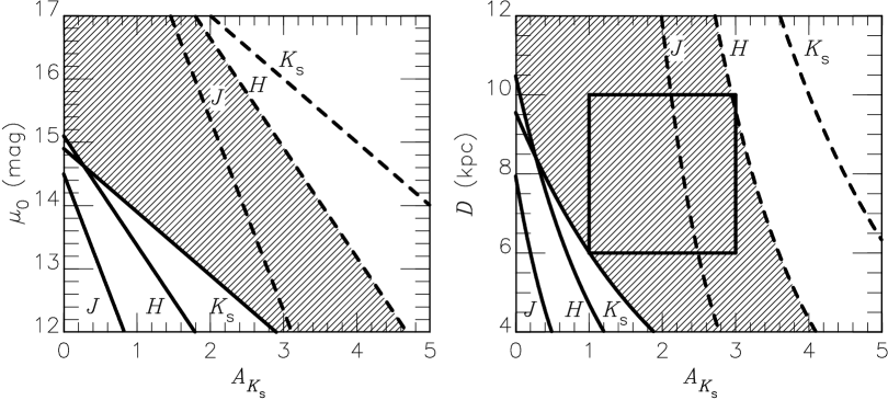
Figure 23: Schematic diagrams to show the parameter space of ${(\mu_{0},~{}A_{K_{\mathrm{s}}})}$ where we can detect Miras in $JHK_{\rm s}$. Dashed curves show the detection limits while solid curves show the saturation limits for $JHK_{\rm s}$ as indicated. In the online version, blue, green and red curves corresponds to the limits in $J$, $H$ and $K_{\mathrm{s}}$ respectively. The two panels plot the same curves, but the $y$ axis in the right one is on a linear scale. The rectangle in the right-hand panel indicates the region we use to estimate the distance to the GC.

We may now proceed to estimate the distance to the GC based on the 100 Miras which have estimated values of $\mu_{0}^{~{}HK}$ between 14 and 15 mag and $A_{K_{\mathrm{s}}}^{~{}HK}$ between 1 and 3 mag. The latter condition is set to avoid selection bias in the ${(\mu_{0},~{}A_{K_{\mathrm{s}}})}$ plane (Fig. 23). One can expect the spread in the estimated distance moduli to accord with the random errors. As shown in Fig. 24, the distribution is well fitted by a Gaussian function with a peak of $\mu_{0}=14.58$ mag. The peak and the width from the fitting are insensitive to the bin width. As already mentioned, random errors for individual Miras are not important when we discuss the distance to the GC because they average out. We take the standard deviation of the mean, viz. 0.02 mag, as the uncertainty in the distance. As a result, the distance modulus to the GC is estimated to be $14.58\pm 0.02~{}{\it(stat.)}\pm 0.11~{}{\it(syst.)}$ mag where the systematic error is included (section 5.3). We denote the linear distance as $R_{0}$ and compare our result, $R_{0}=8.24\pm 0.08\pm 0.42$ kpc, with those of others. When necessary, we re-calculate $R_{0}$ by using $\mu_{\mathrm{LMC}}=18.45$ (if the distance scale in a given work depends on this quantity).

Figure 24: Distribution of the $\mu_{0}^{~{}HK}$ values obtained. The error bar indicates the size of the Poisson noise ($\sqrt{N}$) for each bin. The mean value and width of the fitted Gaussian are indicated in the panel.

In earlier works $R_{0}$ values have been obtained by various methods. That involving stellar orbits around the central black hole Sgr A^∗ is a potentially powerful tool, but there still remains a significant uncertainty. Although Eisenhauer et al. (2005) derived $R_{0}=7.62~{}\pm~{}0.35$ kpc, Trippe et al. (2008) has found that systematic errors neglected in the 2005 paper may change the result. Ghez et al. (2008) obtained $R_{0}=8.0\pm 0.6$ kpc using the same method but based on a different set of data. The same authors obtained $R_{0}=8.07\pm 0.32~{}({\it stat.})\pm 0.13~{}({\it syst.})$ kpc as a statistical parallax using the kinematic properties of several hundred stars around the GC. Results from other methods include: Nishiyama et al. (2006b; $R_{0}=7.52$ kpc, red clump stars), Groenewegen, Udalski & Bono (2008; $R_{0}=7.75$ kpc, type II Cepheids and RR Lyr variables). Our result is similar to the recent results by Trippe et al. (2008) and Ghez et al. (2008).

A few other authors have estimated $R_{0}$ from Miras. Pioneering work was done by Glass & Feast (1982), who conducted near-IR photometry for a few dozen of Miras towards the Baade windows (Sgr I and NGC 6522). Glass et al. (1995) investigated the Miras towards the Sgr I field after further monitoring. Their result was $R_{0}=8.3\pm 0.7$ kpc, but they mentioned that their $R_{0}$ value will increase by 0.2 kpc if the Sgr I field is part of bar at $\sim 45^{\circ}$ to the line of sight. Groenewegen & Blommaert (2005) used the Miras found in the OGLE-II survey fields which cover various lines of sight between $\pm 11^{\circ}$ in $l$, mainly at $b\sim-3.5^{\circ}$. They found that the difference between the distance moduli of the LMC and the Galactic bulge is 3.72 mag, which corresponds to $R_{0}=8.9\pm 0.7$ kpc. They also argued that $R_{0}$ can be as small as 8.35 kpc if one assumes a strong metal dependency of the PLR of Miras. Glass et al. (2009) adopted $R_{0}=8.5$ kpc by comparing their plots of mid-IR magnitudes against periods for pulsating red giants in the LMC and the Galactic bulge including semi-regulars on other sequences. The previous results show rough agreements with ours considering the systematic uncertainties. Note that the fields they examined are at least a few degrees from the GC. Our report is the first to estimate $R_{0}$ by using the Miras towards the GC region itself. Furthermore, the method described here has made it possible to overcome the complicated effects of the interstellar extinction.

5.5 Interstellar extinction

In the course of this work, besides their distances, interstellar extinctions have been estimated for more than 150 Miras. Because we estimate both at the same time, this method has the potential to investigate the extinction in three dimensions directly, revealing how it changes with distance and with line of sight. In spite of the fact that our objects are located at the same distance, the $A_{K_{\mathrm{s}}}$ values cover a large range; the foreground extinction varies strongly with the line of sight. In Fig. 25, we plot the locations of the Miras with $A_{K_{\mathrm{s}}}^{~{}HK}$ values in galactic coordinates. The sizes of the symbols vary according to $A_{K_{\mathrm{s}}}$ as indicated. Whilst circles with various sizes scatter across our observed area, there are some clumps of similar-sized circles.

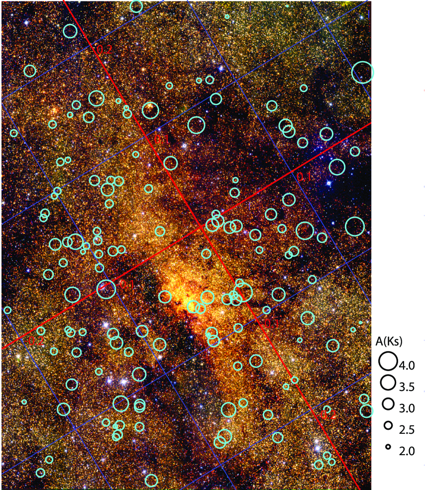
Figure 25: Locations of 143 Miras with $A_{K_{\mathrm{s}}}^{~{}HK}$ obtained. The obtained extinction for each object is indicated by the size of a circle as shown besides the panel.

Figure 26: $A_{K_{\mathrm{s}}}^{~{}HK}$ are plotted against $\mu_{0}^{~{}HK}$.

Fig. 26 plots $A_{K_{\mathrm{s}}}^{~{}HK}$ against $\mu_{0}^{~{}HK}$. The cross indicates the sizes of the errors in the two quantities. Although most of the samples in this study are located at the same distance within the accuracy, there are two sources closer and two further than the main group. The $A_{K_{\mathrm{s}}}$ values obtained for these objects do not show systematic differences from those for the objects with $\mu_{0}=14$–$15$ mag. Unfortunately, the number of tracers with ${(\mu_{0},~{}A_{K_{\mathrm{s}}})}$ is too small to carry out a detailed analysis of the three-dimensional extinction map. Also note that our sample is limited in the ${(\mu_{0},~{}A_{K_{\mathrm{s}}})}$ plane (see Fig. 23). Those with smaller extinction and closer to the Sun will be saturated in our survey, while those with larger extinction and further than the GC are expected to be too faint.

We here estimate the foreground interstellar extinction towards Sgr A^∗ ($l=-0.05575^{\circ},b=-0.04617^{\circ}$). Fig. 27 shows the locations and the $A_{K_{\mathrm{s}}}^{~{}HK}$ values (and $\mu_{0}^{~{}HK}$ in parentheses) for the Miras around Sgr A^∗. Four Miras are located within a radius of 1.5 arcmin, indicated by the dashed circle. It is suggested that the $A_{K_{\mathrm{s}}}$ in the direction towards Sgr A^∗ is approximately 3 mag. Our value corresponds to $A_{V}\sim 45$ mag if we use the extinction coefficient of $A_{V}/A_{K_{\mathrm{s}}}=16$ obtained by Nishiyama et al. (2008). In contrast, extinction values of 2.6 and 2.8 mag in $A_{K_{\mathrm{s}}}$ were obtained toward Sgr A^∗ by Eisenhauer et al. (2005) and Schödel et al. (2007) with higher angular resolution. The latter found that the extinction changes on rather small scales. Our estimate should therefore be regarded as a typical value for a larger region surrounding Sgr A^∗ rather than the value in its precise direction.

Figure 27: This is similar to Fig. 25, but is a closeup for the proximity of Sgr A^∗ which is indicated by the cross. The dashed circle has a radius of 1.5 arcmin and a centre at Sgr A^∗. The $A_{K_{\mathrm{s}}}$ (and $\mu_{0}$ in parentheses) is indicated for each object.

5.6 Mid-IR PLR

Glass et al. (2009) recently investigated the PLR of Miras in the mid-IR range. Their samples consist of the Miras towards the LMC and the NGC 6522 Baade window. Schultheis et al. (2009) fitted the mid-IR PLRs for the G01 Miras around the GC, but there remain large scatters because it was not possible to correct for the variable interstellar extinction.

We have plotted the IRAC magnitudes from Ramírez et al. (2008) against the periods in Fig. 28 for our Miras with ${(\mu_{0},~{}A_{K_{\mathrm{s}}})}$. The fitted linear relations are:

$${[3.6]}=-4.14(\pm 0.20)(\log P-2.3)-7.32(\pm 0.03),$$ (10)

$${[4.5]}=-4.03(\pm 0.20)(\log P-2.3)-7.48(\pm 0.03),$$ (11)

$${[5.8]}=-4.33(\pm 0.24)(\log P-2.3)-7.88(\pm 0.04),$$ (12)

$${[8.0]}=-4.46(\pm 0.33)(\log P-2.3)-8.14(\pm 0.06),$$ (13)

indicated by the solid lines. The residual standard deviations around (10), (11), (12) and (13) are 0.29, 0.29, 0.32 and 0.42 mag, respectively. We here used the $\mu_{0}^{~{}HK}$ and $A_{K_{\mathrm{s}}}^{~{}HK}$ obtained for individual Miras and the extinction coefficients obtained by Nishiyama et al. (2009) to get their absolute magnitudes. Because most of the Miras are found at the same distance within our accuracy, it is also reasonable to use the common distance modulus of 14.58 mag. Even if we do so, the resultant relations do not change from eqs. (10)–(13) including their scatters.

Figure 28: Period-luminosity relation in Spitzer/IRAC filters. The fitted relations are shown as solid lines, while the PLR in Glass et al. (2009) are indicated by dashed lines. Note that they adopted a distance differing from ours by 0.12 mag and we have shifted their fits by this amount.

The scatter around the PLRs that we have found are rather small considering the uncertainty in the ${(\mu_{0},~{}A_{K_{\mathrm{s}}})}$ and the fact that the IRAC magnitudes are based on a single-epoch survey. Uncertainties in the apparent distance moduli in the IRAC filters are estimated at 0.18 mag for individual Miras. The mid-IR amplitudes of Miras are not well known, but those at around 3.5 $\mu\mathrm{m}$ can be as large as in the $K$-band (Feast et al., 1982). These uncertainties suggest that the intrinsic widths of the mid-IR PLRs are narrower than in Fig. 28.

In Fig. 28, we also plot the relation obtained for the C-sequence by Glass et al. (2009) as the dashed lines. Their adopted distance, 14.7 mag for the NGC 6522 field, differs from ours by 0.12 mag and was compensated for before plotting. The slopes agree well with ours. In contrast, the zero points are slightly shifted depending on the wavelength; approximately by $+0.3$ mag for the $\log P$-$[3.6]$ relation and $-0.2$ mag for the $\log P$-$[8.0]$ relation. The reason for the different zero points is unclear. Note that Glass et al. (2009) included semi-regulars and long-period Miras which may have mid-IR excesses in their sample.

5.7 Future prospects

As has been shown, it is possible to obtain both distances and extinctions for Miras with $P=100$–$350$ d by making use of the PLR in two or more near-IR filter bands. This is a very promising tool for investigating Galactic structure. One of the major sources of error is the residual scatter around the PLR. Because we do not have a priori information on how a certain Mira deviates from the fitted PLR, the scatter introduces an uncertainty in the distance estimation. We expect that the intrinsic scatter is smaller than what we found in Fig. 18. The magnitudes used in Fig. 18 are intensity means of ten-epoch monitoring data, which can introduce an uncertainty as large as 0.1 mag based on the Monte-Carlo simulation presented in section 3.3. The scatter should get smaller if we take mean magnitudes more accurately.

The uncertainty in the zero point of the PLR and the possible population effect may also introduce significant errors; it is important to note however that these will be systematic ones. Future parallax observations of Miras in the solar neighbourhood may reduce these uncertainties. For example, Vlemmings et al. (2003) and Vlemmings & van Langevelde (2007) have reported the parallaxes for five Miras with OH maser emission. As reviewed by Whitelock et al. (2008), their results are consistent with the PLR of the LMC Miras within their uncertainties, which are still not small enough to draw strong conclusions about the zero point or the population effect. VERA, a Japanese VLBI project, is one of the most promising projects for calibrating the PLR of Miras in the Galaxy (Nakagawa et al. 2008, 2009). However, the use of radio parallaxes is constrained by the small numbers of Miras with maser emission in the short-period range, say $P\leq 300$ d. In our method for deriving the distance and the extinction, we make use of short-period Miras to avoid the effects of circumstellar extinction and/or hot-bottom-burning. In this regard, future optical and near-IR astrometric satellites such as GAIA (Turon et al., 2008) and JASMINE (Gouda et al., 2008) can play a fundamental role in the calibration of the PLR.

6 Summary

This paper reports 1364 variable stars in a $20\arcmin\times 30\arcmin$ region around the GC found through our near-IR survey covering seven years. We have obtained periods for 549 objects, most of which are considered to be Miras. We have described a method for obtaining distances and extinctions for Miras with periods between 100 and 350 d by making use of their PLR. The technique depends on knowing mean magnitudes in two or more filters in the near IR. A particular effort has been made to assess the uncertainties; the random error is about 0.2 mag in the distance modulus for an individual Mira, while the systematic error is about 0.11 mag, mainly originating from a combination of uncertainties in the LMC distance ($\pm 0.05$ mag), the extinction coefficient ($\pm 0.07$ mag) and the population effect on the PLR ($\pm 0.07$ mag).

We obtained the distances of 143 Miras by using the $H$- and $K_{\mathrm{s}}$-band mean magnitudes. They are strongly concentrated to the GC, whose distance modulus was estimated at 14.58 mag. The statistical error is 0.02 mag from the standard deviation of the mean and the systematic error is again 0.11 mag. Our statistical error is the smallest among estimates to date, and the distance we have obtained shows rough agreement with recent results from other methods, within the systematic uncertainties. The PLR of Miras is shown to be a powerful tool for studying Galactic structure, although there remains a significant systematic error. It is expected that better calibration of the PLR will improve the accuracy of the method; this may be achieved by parallax projects such as VERA and GAIA.

We also have discussed the distribution of the interstellar extinction towards the GC. Because we can estimate distances and extinctions for individual Miras, they can be used as tracers to reveal three-dimensional structure. It is possible to study how the extinction changes with distance along various lines of sight, although the low space density of Miras may prevent us from investigating small structures. We have confirmed that the extinction towards the GC region varies complicatedly between 1.5 and 4 mag in $A_{K_{\mathrm{s}}}$, excepting towards extremely dark nebulae, and we have estimated the extinction towards the Sgr A^∗ region to be $A_{K_{\mathrm{s}}}\sim 3$ mag.

References

- Babusiaux & Gilmore (2005) Babusiaux C., Gilmore G., 2005, MNRAS, 358, 1309
- Clement et al. (2008) Clement C. M., Xu X., Muzzin A. V., 2008, AJ, 135, 83
- Eisenhauer et al. (2005) Eisenhauer F. et al., 2005, ApJ, 628, 246
- Feast (1996) Feast M. W., 1996, MNRAS, 278, 11
- Feast (2004) Feast M. W., 2004, in Kurts D. W., Pollard K. R., eds, ASP Conf. Ser., Vol. 310, Variable Stars in the Local Group, Astron. Soc. Pac., San Francisco, p. 304
- Feast (2009) Feast M. W., 2009, in Ueta T., Matsunaga N., Ita Y., eds., AGB stars and related phenomena. Osaka, OM Publishing Co. Ltd., p. 48, preprint (arXiv:0812.0250)
- Feast et al. (1982) Feast M. W., Robertson B. S. C., Catchpole R. M., Lloyd Evans T., Glass I. S., Carter B. S., 1982, MNRAS, 201, 439
- Feast et al. (1989) Feast M. W., Glass I. S., Whitelock P. A., Catchpole R. M., 1989, MNRAS, 241, 375
- Frogel et al. (1999) Frogel J. A., Tiede G. P., Kuchinski L. E., 1999, AJ, 117, 2296
- Ghez et al. (2008) Ghez A. M. et al., 2008, ApJ, 689, 1044
- Glass et al. (1990) Glass I. S., Whitelock P. A., Catchpole R. M., Feast M. W., Laney C. D., 1990, SAAO Circulars No 14, p. 63
- Glass et al. (2001) Glass I. S., Matsumoto S., Carter B. S., Sekiguchi K., 2001, MNRAS, 321, 77 (G01)
- Glass et al. (2002) Glass I. S., Matsumoto S., Carter B. S., Sekiguchi K., 2002, MNRAS, 336, 1390
- Glass et al. (2009) Glass I. S., Schultheis M., Blommaert J. A. D. L., Sahai R., Stute M., Uttenthaler S., 2009, MNRAS, 395, L11
- Glass et al. (1995) Glass I. S., Whitelock P. A., Catchpole R. M., Feast M. W., 1995, MNRAS, 273, 383
- Glass & Lloyd Evans (1981) Glass I. S., Lloyd Evans T., 1981, Nature, 291, 303
- Glass & Lloyd Evans (2003) Glass I. S., Lloyd Evans T., 2003, MNRAS, 343, 67
- Glass & Feast (1982) Glass I. S., Feast M. W., 1982, MNRAS, 198, 199
- Gosling et al. (2009) Gosling A. J., Bandyopadhyay R. M., Blundell K. M., 2009, MNRAS, 394, 2247
- Gouda et al. (2008) Gouda N., Kobayashi Y., Yamada Y., Yano T., 2008, IAUS, 248, 248
- Grocholski et al. (2007) Grocholski A. J., Sarajedini A., Olsen K. A. G., Tiede G. P., Mancone C. L., 2007, AJ, 134, 680
- Groenewegen (2004) Groenewegen M. A. T., 2004, A&A, 425, 595
- Groenewegen & Blommaert (2005) Groenewegen M. A. T., Blommaert J. A. D. L., 2005, A&A, 443, 143
- Groenewegen et al. (2008) Groenewegen M. A. T., Udalski A., Bono G., 2008, A&A, 481, 441
- Ita et al. (2004a) Ita Y. et al., 2004a, MNRAS, 347, 720
- Ita et al. (2004b) Ita Y. et al., 2004b, MNRAS, 353, 705 (I04)
- Lebzelter et al. (2002) Lebzelter T., Schultheis M., Melchior A. L., 2002, A&A, 393, 573
- Lindqvist et al. (1992) Lindqvist M., Habing H. J., Winnberg A., 1992, A&A, 259, 118
- Matsunaga et al. (2005) Matsunaga N., Fukushi H., Nakada Y., 2005, MNRAS, 364, 117 (M05)
- Matsunaga et al. (2009) Matsunaga N., Feast M. W., Menzies J. W., 2009, MNRAS, in press (arXiv:0904.4701)
- Menzies et al. (2008) Menzies J. W., Feast M. W., Whitelock P. A., Olivier E., Matsunaga N., da Costa G., 2008, MNRAS, 385, 1045
- Nagashima et al. (1999) Nagashima C., et al. 1999, in ed. T. Nakamoto, Proceedings of Star Formation 1999, Star Formation, Nagoya, p. 397
- Nagayama et al. (2003) Nagayama T. et al., 2003, in eds. M. Iye & A. F. M. Moorwood, Instrument Design and Performance for Optical/Infrared Ground-based Telescopes, SPIE Vol. 4841, p. 459
- Nakagawa et al. (2008) Nakagawa A. et al., 2008, PASJ, 60, 1013
- Nakagawa et al. (2009) Nakagawa A. et al., 2009, in Ueta T., Matsunaga N., Ita Y., eds., AGB stars and related phenomena. Osaka, OM Publishing Co. Ltd., p. 58
- Nakanishi & Sofue (2003) Nakanishi H., Sofue Y., 2003, PASJ, 55, 191
- Nakanishi & Sofue (2006) Nakanishi H., Sofue Y., 2006, PASJ, 58, 847
- Nishiyama et al. (2005) Nishiyama S. et al., 2005, ApJ, 621, L105
- Nishiyama et al. (2006a) Nishiyama S. et al., 2006a, ApJ, 638, 839
- Nishiyama et al. (2006b) Nishiyama S. et al., 2006b, ApJ, 647, 1093
- Nishiyama et al. (2008) Nishiyama S., Nagata T., Tamura M., Kandori R., Hatano H., Sato S., Sugitani K., 2008, ApJ, 680, 1174
- Nishiyama et al. (2009) Nishiyama S., Tamura M., Hatano H., Kato D., Tanabé T., Sugitani K., Nagata T., 2009, ApJ, 696, 1407
- Persson et al. (1998) Persson S. E., Murphy D. C., Krzeminski W., Roth M., Rieke M. J., 1998, AJ, 116, 2475
- Ramírez et al. (2008) Ramírez S. V., Arendt R. G., Sellgren K., Stolovy S. R., Cotera A., Smith H. A., Yusef-Zadeh F., 2008, ApJS, 175, 147
- Rattenbury et al. (2007) Rattenbury N. J., Mao S., Sumi T., Smith M. C., MNRAS, 378, 1064
- Rejkuba (2004) Rejkuba M., 2004, A&A, 413, 903
- Schödel et al. (2007) Schödel R., et al., 2007, A&A, 469, 125
- Schultheis et al. (2004) Schultheis M., Glass I. S., Cioni M.-R., 2004, A&A, 427, 945
- Schultheis et al. (2009) Schultheis M., Sellgren K., Ramírez S. V., Stolovy S., Ganesh S., Glass I. S., Girardi L., 2009, A&A, 495, 157
- Skrutskie et al. (2006) Skrutskie M. F. et al., 2006, AJ, 131, 1163
- Serabyn & Morris (1996) Serabyn E., Morris M., 1996, Nature, 382, 602
- Trippe et al. (2008) Trippe S. et al., 2008, A&A, 492, 419
- Tabur (2007) Tabur V., 2007, PASA, 24, 189
- Turon et al. (2008) Turon C., Primas F., Binney J., Chiappini C., Drew J., Helmi A., Robin A. C., Ryan S. G., 2008, ESA-ESO Working Group report #4: ESA-ESO Working Group on Galactic Populations, Chemistry and Dynamics (ESA and ESO)
- Udalski et al. (1997) Udalski A., Kubiak M., Szymański M., 1997, Acta Astron., 47, 319
- van Leeuwen et al. (2007) van Leeuwen F., Feast M. W., Whitelock P. A., Laney C. D., 2007, MNRAS, 379, 723
- Vlemmings et al. (2003) Vlemmings W. H. T., van Langevelde H. J., Diamond P. J., Habing H. J., Schilizzi R. T., 2003, A&A, 407, 213
- Vlemmings & van Langevelde (2007) Vlemmings W. H. T., van Langevelde H. J., 2007, A&A, 472, 547
- Whitelock et al. (1991) Whitelock P. A., Feast M. W., Catchpole, R. M., 1991, MNRAS, 248, 276
- Whitelock et al. (2003) Whitelock P. A. Feast M. W., van Loon J. Th., Zijlstra A. A., 2003, MNRAS, 342, 86
- Whitelock et al. (2000) Whitelock P. A., Marang F., Feast M. W., 2000, MNRAS, 319, 728
- Whitelock et al. (1994) Whitelock P. A., Menzies J. W., Feast M. W., Marang F., Carter B., Roberts G., Catchpole R., Chapman J., 1994, MNRAS, 267, 711
- Whitelock et al. (2009) Whitelock, P. A., Menzies J. W., Feast M. W., Matsunaga N., Tanabé T., Ita Y., 2009, MNRAS, 394, 795
- Whitelock et al. (2008) Whitelock, P. A., Menzies J. W., Feast M. W., van Leeuwen F., 2008, MNRAS, 386, 313
- Wood et al. (1998) Wood P. R., Habing H. J., McGregor P. J., 1998, A&A, 336, 925
- Wood et al. (1998) Wood P. R. et al., 1999, IAUS, 191, 151
- Woźniak et al. (2002) Woźniak, P. R., Udalski, A., Szymanski, M., Kubiak, M., Pietrzynski, G., Soszynski, I., Zebrun, K., 2002, Acta Astron., 52, 129.