On Cyclic and Nearly Cyclic Multiagent Interactions
in the Plane

Abstract

We discuss certain types of cyclic and nearly cyclic interactions among $N$ “point”-agents in the plane, leading to formations of interesting limiting geometric configurations. Cyclic pursuit and local averaging interactions have been analyzed in the context of multi-agent gathering. In this paper, we consider some nearly cyclic interactions that break symmetry leading to factor circulants rather than circulant interaction matrices.

1 Introduction

Consider a “swarm” or “pack” of $N$ robots in the plane, denoted by $\mathcal{P}_{0},\mathcal{P}_{1},\ldots\mathcal{P}_{N-1}$ which can all see each other and are aware of the other robot’s identities (i.e., can distinguish them). We shall define the rules of interaction specifying how each robot $\mathcal{P}_{k}$ moves in response to the (evolution in time of the) configuration of the entire swarm. Therefore denoting $\mathcal{P}_{k}$’s location at time $t$ to be $\mathcal{P}_{k}(t)=x_{k}(t)+iy_{k}(t)$ (a complex number), we assume that we can write the swarm evolution equations as follows:

$$\frac{d\mathcal{P}_{k}(t)}{dt} = \Phi_{k}^{(C)}\{\mathcal{P}_{s}(\xi)|_{s=0,1,\ldots N-1};\xi\leq t\}$$

$$\textrm{or}\ \ \mathcal{P}_{k}(t+1) = \Phi_{k}^{(D)}\{\mathcal{P}_{s}(\xi)|_{s=0,1,\ldots N-1};\xi\leq t\}$$ (1)

depending on whether the temporal evolution is continuous $(C)$ or discrete $(D)$. So far the $\Phi$-operators are not specified, and in fact they could be quite involved in general. The operator $\Phi_{k}^{(C)}$ provides an instantaneous velocity vector for agent $\mathcal{P}_{k}$ in response to the locations of the other agents in the swarm, while $\Phi_{k}^{(D)}$ will yield the next location for $\mathcal{P}_{k}$ in a synchronous discrete timed evolution. These operators should produce the same motion if we decide to look at the agents in different frames of reference, i.e., re-encode their locations using transformed coordinates, hence the resulting equations should be at least similarity invariant, and maybe even affine invariant. The requirement to have the same evolution equation in arbitrarily similarity (i.e., scaled Euclidean) or affine transformed coordinates clearly imposes restrictions on the $\Phi$ operators and some of these will be discussed in the sequel.

An important class of operators are the linear memoryless ones which have the form

$$\Phi_{k}\{\mathcal{P}_{0},\mathcal{P}_{1},\ldots\mathcal{P}_{N-1}\}=\sum_{l=0}^{N-1}m^{k}_{l}(t)\mathcal{P}_{l}(t)$$

where $m_{l}^{k}(t)$ are some (complex) numbers, varying perhaps in time. In this case, Equation (1) describes a linear (generally time varying) system’s state evolution, and there is a wealth of theory dealing with such systems in the control and signal processing literature. Here we shall mainly be concerned with a special class of (constant) linear Toeplitz operators of the form

$$\Phi_{k}\{\mathcal{P}_{0},\mathcal{P}_{1},\ldots\mathcal{P}_{N-1}\}=\sum_{l=0}^{N-1}\lambda^{\textrm{Ind}[(l-k)<0]}m_{(l-k)\textrm{mod}~{}N}\mathcal{P}_{l}(t)$$ (2)

where $\lambda$ is some complex number, and

$$\left\{\begin{array}[]{c}m_{-1}\equiv m_{N-1}\textrm{mod}~{}N\\ m_{-k}\equiv m_{N-k}\textrm{mod}~{}N\end{array}\right.\textrm{and}\ \ \textrm{Ind}[a<0]=\left\{\begin{array}[]{lll}1&if&a<0\\ 0&if&a\geq 0\end{array}\right..$$

Writing out explicitly $\Phi_{k}\{\mathcal{P}_{0},\ldots,\mathcal{P}_{N-1}\}$ for $k=0,\ldots,N-1$ in matrix form and denoting

$$\mathbf{P}(t)=\left[\begin{array}[]{c}\mathcal{P}_{0}(t)\\ \vdots\\ \mathcal{P}_{N-1}(t)\end{array}\right],$$

the swarm’s evolution dynamics becomes

$$\left(\frac{d}{dt}\mathbf{P}(t)~{}\textrm{or}\right)\mathbf{P}(t+1) = \Phi\mathbf{P}(t)$$ (3)

$$= \left[\begin{array}[]{ccccl}m_{0}&m_{1}&m_{2}&\ldots&m_{N-1}\\ \lambda m_{N-1}&m_{0}&m_{1}&\ldots&m_{N-2}\\ \lambda m_{N-2}&\lambda m_{N-1}&m_{0}&\ldots&\ldots\\ \vdots&\vdots&\ldots&\ddots&\ldots\\ \lambda m_{1}&\lambda m_{2}&\ldots&\lambda m_{N-1}&m_{0}\end{array}\right]\mathbf{P}(t).$$ (9)

Note here that if $\lambda=1$, the matrix is a special Toeplitz-circulant matrix, otherwise it is a generalization of a circulant called a $\lambda$-factor, or $\lambda$-circulant matrix. Such matrices arise in several applications, such as linear systems theory [8, 10], linear algebra [1], geometry [5, 13, 14], and in connection with inverses of Toeplitz matrices [7, 9, 4], coding theory [6] and linear systems of differential equations [17]. In case of $\lambda=1$, i.e., when the operator $\Phi$ is Toeplitz-circulant, we have that all the robotic agents perform “cyclically” the same operation, i.e. agent $\mathcal{P}_{k}$ will determine its next location (or its velocity) according to the same weighted average performed on $\mathcal{P}_{k},\mathcal{P}_{k+1},\ldots\mathcal{P}_{(k+N)\textrm{mod}N}$ (in this order), i.e.

$$\left\{\begin{array}[]{l}\mathcal{P}_{k}(t+1)\\ \textrm{or }\frac{d}{dt}\mathcal{P}_{k}(t)\end{array}\right\} = [m_{0},m_{1},\ldots m_{N-1}]\left[\begin{array}[]{l}\mathcal{P}_{k}(t)\\ \mathcal{P}_{k+1}(t)\\ \vdots\\ \mathcal{P}_{(k+N)\textrm{mod}~{}N}(t)\end{array}\right]$$ (16)

which can be rewritten as

$$\left\{\begin{array}[]{l}\mathcal{P}_{k}(t+1)\\ \textrm{or }\frac{d}{dt}\mathcal{P}_{k}(t)\end{array}\right\} = \bar{m}\left[\begin{array}[]{ccrccccc}0&0&0&1&{}^{(k^{th}place)}&\ldots&0\\ &&&&1&&\\ &&&&&1&\\ &&&&&&\ddots\\ 1&&&&&&\\ &1&&&&&\\ &&1&&&\ldots&0\\ 0&\ldots&&1&\ldots&0&0\end{array}\right]\left[\begin{array}[]{l}\mathcal{P}_{0}(t)\\ \mathcal{P}_{1}(t)\\ \vdots\\ \mathcal{P}_{N-1}(t)\end{array}\right]$$ (31)

$$= \bar{m}\mathbf{Z}^{k-1}\cdot\mathbf{P}(t)$$ (32)

where

$$\mathbf{Z}\triangleq\left[\begin{array}[]{ccccc}0&1&&&0\\ \vdots&0&1&&\\ \vdots&&0&1&\\ 0&&&0&1\\ 1&0&\cdots&&0\end{array}\right]\mbox{ and }\bar{m}=[m_{0},m_{1},\ldots m_{N-1}].$$

This special case, with a circulant matrix $\Phi$, was extensively analyzed before in the context of polygon smoothing evolutions and cyclic pursuits for robotic gathering and formation control, see e.g. [5, 13, 14, 3, 2, 12, 11, 7].

Note that invariance requirements impose some conditions on the linear evolution operators, as we now discuss. If $\mathbf{P}(t)$ is described by the evolution equations

$$\frac{d}{dt}\mathbf{P}(t) = \Phi^{(C)}\mathbf{P}(t)$$

$$\mbox{or }\mathbf{P}(t+1) = \Phi^{(D)}\mathbf{P}(t)$$

from some initial location $\mathbf{P}(0)=\mathbf{P}(t=0)$, and if we re-encode the agents’ positions via a general similarity transformation of the form

$$\mathbf{P}^{\prime}(t)\triangleq\rho\mathbf{P}(t)+\tau{\bf 1}$$

where $\rho$ and $\tau$ are some complex numbers and ${\bf 1}=[1,\ldots,1]^{T}$, we shall have for $\mathbf{P}^{\prime}(t)$:

• in the continuous case

  $$\frac{d}{dt}\mathbf{P}^{\prime}(t) \triangleq \frac{d}{dt}\left(\rho\mathbf{P}(t)+\tau{\bf 1}\right)$$

  $$= \rho\frac{d}{dt}\mathbf{P}(t)$$

  $$= \rho\Phi^{(C)}\mathbf{P}(t)$$

  which is equal to $\Phi^{(C)}\left(\rho\mathbf{P}(t)+\tau{\bf 1}\right)$ only if $\Phi^{(C)}{\bf 1}={\bf 0}$.

• in the discrete case

  $$\mathbf{P}^{\prime}(t+1) \triangleq \rho\mathbf{P}(t+1)+\tau{\bf 1}$$

  $$= \rho\Phi^{(D)}\mathbf{P}(t)+\tau{\bf 1}$$

  which is equal to $\Phi^{(D)}\left(\rho\mathbf{P}(t)+\tau{\bf 1}\right)$ only if $\Phi^{(D)}{\bf 1}={\bf 1}$.

Hence the $\Phi$-matrices that describe linear, time-invariant evolutions need to obey the conditions $\Phi^{(C)}{\bf 1}={\bf 0}$ or $\Phi^{(D)}{\bf 1}={\bf 1}$ in order to have Euclidean or similarity invariant evolutions. In some of our examples, these conditions cannot be satisfied. However, note that any $N\times N$ matrix $\Phi$ may be embedded in an $(N+1)\times(N+1)$ matrix ${\bf\Phi}$ as follows

$$\left[\begin{array}[]{cc}\Phi&{\bf s}\\ {\bf 0}&z\end{array}\right]\left[\begin{array}[]{c}1\\ \vdots\\ 1\end{array}\right]=\left[\begin{array}[]{c}\Phi{\bf 1}+{\bf s}\\ z\end{array}\right]$$

and selecting either $z=0$ and ${\bf s}=-\Phi{\bf 1}$ or $z=1$, we obtain a ${\bf\Phi}$ matrix that describes an invariant evolution of a multi-agent system with an additional agent $\mathcal{P}_{B}$ whose position is stationary ($\frac{d}{dt}\mathcal{P}_{B}=0$ or $\mathcal{P}_{B}(t+1)=\mathcal{P}_{B}(t)$). This additional agent will act as a “beacon” or a set reference point, for the description of the swarm of agents. In this case, setting $\mathcal{P}_{B}=(0,0)$, the evolution of the rest of the agents will be described by the original matrix $\Phi$. Note that the spatial location of the fixed $\mathcal{P}_{B}$ in the plane may be determined according to the initial location of the agents of the swarm. A good example is the geometric and affine invariant decision that can be made by each agent independently to set $\mathcal{P}_{B}$, and hence the origin of its Cartesian coordinate system, at the centroid of the agent location constellation at $t=0$. This will make the swarm evolution entirely autonomous. However, an external setting of the location of $\mathcal{P}_{B}$ might be useful in controlling the swarm and steering it toward a desired place in the environment. One might even desire to move $\mathcal{P}_{B}$ in time and make the swarm move accordingly, by tracking the beacon point in addition to its own internal dynamics controlled by $\Phi$.

2 Analyzing Swarm Evolution via Mode Decoupling

Circulant, and $\lambda$-factor circulant matrices have very special structures and this allows us to diagonalize them, essentially by Fourier transform methods. Let us see, in general, how diagonalization yields a way to analyze the evolution of the constellation of robots by decoupling it into independently evolving modes. Indeed assume that the time-invariant matrix $\Phi$ can be diagonalized (for example when $\Phi$ has distinct eigenvalues, hence a full set of orthonormal eigenvectors), as follows

$$\Phi=T^{-1}DT$$

where $D=\mbox{Diag}[d_{0},d_{1}\ldots d_{N-1}]$ displays the eigenvalues of $\Phi$ and the columns of $T^{-1}$ are the (right) eigenvectors. Now we have that

$$\left.\begin{array}[]{cc}&\mathbf{P}(t+1)\\ \textrm{or}&\\ &\frac{d}{dt}\mathbf{P}(t)\end{array}\right\}=T^{-1}DT\mathbf{P}(t)$$

and hence

$$\left.\begin{array}[]{cc}&T\mathbf{P}(t+1)\\ &\frac{d}{dt}(T\mathbf{P}(t))\end{array}\right\}=D(T\mathbf{P}(t)).$$

In terms of the transformed vector $\widetilde{\mathbf{P}}(t)\triangleq T\mathbf{P}(t)$, the evolution is a decoupled evolution controlled explicitly by the (constant) eigenvalues [10]. Indeed, we have

$$\widetilde{\mathbf{P}}(t)={\left[\begin{array}[]{cccc}d_{o}^{t}&&&\\ &d_{1}^{t}&0&\\ &&\ddots&\\ &0&&d_{N-1}^{t}\end{array}\right]\widetilde{\mathbf{P}}(0)}_{\textrm{(discrete case)}}$$

or

$$\widetilde{\mathbf{P}}(t)={\left[\begin{array}[]{cccc}e^{d_{0}t}&&&\\ &e^{d_{1}t}&0&\\ &&\ddots&\\ &0&&e^{d_{N}t}\end{array}\right]\widetilde{\mathbf{P}}(0)}_{\textrm{(continous case)}}.$$

Therefore diagonalization enables the explicit solution of the swarm evolution, in the case the $\Phi$ matrix is time invariant and has a full set of orthonormal eigenvectors. As we shall see below, $\lambda$-factor circulants are a family of matrices that enable both a nice physical interpretation in terms of cyclic and symmetric interactions among similar agents and an explicit diagonalization via discrete Fourier transform matrices.

3 Diagonalization of Factor Circulants

Factor circulant matrices are very special in that they provide explicit formulae for the diagonalizing transforms and for their eigenvalues. This enables us to analyze in detail the behavior of multiagent interactions when these are cyclic or “nearly” cyclic, and fully describe the limiting behaviors of the swarm. For circulants, we have the following results. Consider the unitary Fourier transform matrix

$$[\mathbf{FT}] \triangleq \frac{1}{\sqrt{N}}\left[\begin{array}[]{llll}w^{0}&w^{0}&\ldots&w^{0}\\ w^{0}&w^{1}&\ldots&w^{N-1}\\ \vdots&\vdots&&\vdots\\ w^{0}&w^{N-1}&\ldots&w^{(N-1)(N-1)}\end{array}\right]$$

$$= \frac{1}{\sqrt{N}}\left[w^{(k-1)(l-1)}\right]_{k,l=1,\ldots,N}$$

where $w=e^{-i\frac{2\pi}{N}}$ is an $N^{th}$ root of unity. Then $\mathbf{C}$ is a Toeplitz-circulant matrix if and only if

$$\mathbf{C}[\mathbf{FT}]=[\mathbf{FT}]\left[\begin{array}[]{cccc}\mu_{o}&&&\\ &\mu_{1}&0&\\ &&\ddots&\\ &0&&\mu_{N-1}\end{array}\right]$$

where $\mu_{0},\mu_{1},\ldots,\mu_{N-1}$ are the eigenvalues of $\mathbf{C}$ and are given by

$$\mu_{l}=\sum_{k=0}^{N-1}c_{k}e^{-i\frac{2\pi}{N}kl}.$$

Hence

$$[\mathbf{FT}]^{*}\mathbf{C}[\mathbf{FT}]=\textrm{Diag}[\mu_{0},\mu_{1},\ldots,\mu_{N-1}]$$

and

$$\mathbf{C}=[\mathbf{FT}]\textrm{Diag}[\mu_{0},\mu_{1},\ldots,\mu_{N-1}][\mathbf{FT}]^{*}.$$

To summarize the remarkable properties of circulants, we can state that they are (1) diagonalized by the discrete Fourier Transform, (2) they all commute, (3) their products are circulants, (4) their sums are circulants too, and (5) their inverses/pseudoinverses are circulants, and are readily found [9]. In fact, many of the wonders of modern signal processing algorithms, and linear, time invariant systems theory stem from the above properties.

The corresponding, and equally remarkable properties of $\lambda$-circulants are, however, much less known and applied. Suppose we consider the following operation on a circulant $\mathbf{C}=\mathbf{C}_{[c_{0},c_{1},\ldots,c_{N-1}]}$:

$$\mathbf{W}=\left[\begin{array}[]{cccc}a_{o}&&&\\ &a_{1}&0&\\ &&\ddots&\\ &0&&a_{N-1}\end{array}\right]\mathbf{C}_{[c_{0},c_{1},\ldots,c_{N-1}]}\left[\begin{array}[]{cccc}b_{o}&&&\\ &b_{1}&0&\\ &&\ddots&\\ &0&&b_{N-1}\end{array}\right]$$

i.e. $\mathbf{W}$ is obtained by pre- and post multiplying $\mathbf{C}$ by two diagonal matrices. It is easy to see that we have

$$\mathbf{W}\!=\mathbf{C}_{[c_{0},c_{1},\ldots,c_{N-1}]}\odot\left[\begin{array}[]{llll}a_{0}b_{0}&a_{0}b_{1}&\ldots&a_{0}b_{N-1}\\ a_{1}b_{0}&a_{1}b_{1}&\ldots&a_{1}b_{N-1}\\ \vdots&\vdots&&\vdots\\ a_{N-1}b_{0}&a_{N-1}b_{1}&\ldots&a_{N-1}b_{N-1}\end{array}\!\!\right]\!=\mathbf{C}\odot\mathbf{M}$$

where $\odot$ stands for the Schur Hadamard multiplication (or a “masking” operation) which multiplies matrices element-wise, and

$$\mathbf{M}\triangleq[a_{k}b_{l}]_{k,l=0,\ldots,n-1}.$$

For matrices of the type $\mathbf{W}$, we have that they inherit interesting diagonalization properties from the original circulant $\mathbf{C}$. The matrix $\mathbf{W}$ is a circulant matrix that is modified by a highly structured masking matrix $\mathbf{M}$ and we have that

$$\mathbf{W}=\textrm{Diag}[a_{0},\ldots,a_{N-1}][\mathbf{FT}]\textrm{Diag}[\mu_{0},\ldots,\mu_{N-1}][\mathbf{FT}]^{*}\textrm{Diag}[b_{0},\ldots,b_{N-1}].$$

However, since the masking matrix is neither circulant nor Toeplitz, we shall have to consider some special cases for the $\{a_{0},a_{1},\ldots,a_{N-1}\}$ and $\{b_{0},b_{1},\ldots,b_{N-1}\}$ sequences. First of all, note that the factorization above will be of the form

$$\mathbf{W}=\mathbf{U}\left[\begin{array}[]{ccc}\mu_{0}&&\\ &\ddots&\\ &&\mu_{N-1}\end{array}\right]\mathbf{U}^{-1}$$

if and only if

$$(\textrm{Diag}[a_{0},a_{1},\ldots,a_{N-1}][\mathbf{FT}])^{-1} = [\mathbf{FT}]^{*}\textrm{Diag}[b_{0},b_{1},\ldots,b_{N-1}]$$

$$\iff[\mathbf{FT}]^{*}\textrm{Diag}[a_{0}^{-1},a_{1}^{-1},\ldots,a_{N-1}^{-1}] = [\mathbf{FT}]^{*}\textrm{Diag}[b_{0},b_{1},\ldots,b_{N-1}]$$

or $b_{k}=a^{-1}_{k}$, and $\mathbf{U}$ will further be unitary if also $b_{k}=a^{*}_{k}$, implying that $a_{k}=e^{j\alpha_{k}}$ and $b_{k}=e^{-j\alpha_{k}}=a_{k}^{*}$. In this case the masking-matrix multiplying $\mathbf{C}$ will be $[e^{j\alpha_{k}}e^{-j\alpha_{l}}]=[e^{j(\alpha_{k}-\alpha_{l})}]_{k,l=0,\ldots,N-1}$.

The most interesting particular cases of $\{a_{0},a_{1},\ldots,a_{N-1}\}$ and $\{b_{0},b_{1},\ldots,b_{N-1}\}$ arise when we have $a_{k}=\gamma^{k}$ and $b_{k}=\gamma^{-k}$, $k=0,1\ldots,N-1$, for some real or imaginary $\gamma$. In this case, we have in general

$$\mathbf{M} = \left[\begin{array}[]{lllll}1&\gamma^{-1}&\gamma^{-2}&\ldots&\gamma^{-(N-1)}\\ \gamma&1&\gamma^{-1}&\ldots&\gamma^{-(N-1)+1}\\ \gamma^{2}&\gamma&1&\ldots&\gamma^{-(N-1)+2}\\ \vdots&\vdots&\ddots&\ddots&\vdots\\ \gamma^{N-1}&\gamma^{N-2}&\ldots&\gamma&1\end{array}\right]$$

$$= \textrm{Circ}_{[1,\gamma^{-1},\ldots,\gamma^{-(N-1)}]}\odot\left[\begin{array}[]{ccccc}1&1&1&1&1\\ \gamma^{N}&1&1&1&1\\ \gamma^{N}&\gamma^{N}&1&1&1\\ \vdots&&&\ddots&\\ \gamma^{N}&\gamma^{N}&\ldots&\gamma^{N}&1\end{array}\right]$$

where $\textrm{Circ}_{[1,\gamma^{-1},\ldots,\gamma^{-(N-1)}]}$ is given by

$$\left[\begin{array}[]{ccccc}1&\gamma^{-1}&\gamma^{-2}&\ldots&\gamma^{-(N-1)}\\ \gamma^{-(N-1)}&1&\gamma^{-1}&\ldots&\gamma^{-(N-1)+1}\\ \gamma^{-(N-1)+1}&\gamma^{-(N-1)}&1&\ldots&\\ \vdots&\vdots&\ddots&1&\vdots\\ \gamma^{-(N-1)+(N-2)}&&\ldots&\gamma^{-(N-1)}&1\end{array}\right].$$

Hence the matrix $\mathbf{W}=\mathbf{C}\odot\mathbf{M}$ becomes

$$\mathbf{W}=\mathbf{C}_{[c_{0},\ldots,c_{N-1}]}\odot\textrm{Circ}_{[1,\gamma^{-1},\ldots,\gamma^{-(N-1)}]}\odot\left[\begin{array}[]{ccccc}1&1&1&1&1\\ \gamma^{N}&1&1&1&1\\ \gamma^{N}&\gamma^{N}&1&1&1\\ \vdots&&&\ddots&\\ \gamma^{N}&\gamma^{N}&\ldots&\gamma^{N}&1\end{array}\right]$$

which clearly is a $\lambda(=\gamma^{N})$- circulant matrix.

To summarize, we have the following result: A $\lambda$-circulant matrix $\mathbf{W}$, denoted by

$$\mathbf{W}=\left[\begin{array}[]{ccccc}m_{0}&m_{1}&m_{2}&\ldots&m_{N-1}\\ \lambda m_{N-1}&m_{0}&m_{1}&\ldots&m_{N-2}\\ \lambda m_{N-2}&\lambda m_{N-1}&m_{0}&\ldots&\ldots\\ \vdots&\vdots&\ldots&\ddots&\ldots\\ \lambda m_{1}&\lambda m_{2}&\ldots&\lambda m_{N-1}&m_{0}\end{array}\right]$$

can be rewritten as

$$\mathbf{W}=\textrm{Circ}_{[m_{0},m_{1}\gamma,m_{2}\gamma^{2},\ldots,m_{N-1}\gamma^{N-1}]}\odot\textrm{Circ}_{[1,\gamma^{-1},\ldots,\gamma^{-(N-1)}]}\odot\Lambda$$

with

$$\Lambda=\left[\begin{array}[]{ccccc}1&1&1&\ldots&1\\ \lambda&1&1&\ldots&1\\ \lambda&\lambda&1&\ldots&1\\ \vdots&\vdots&\lambda&1&\vdots\\ \lambda&\lambda&\ldots&\lambda&1\end{array}\right]\textrm{and }\gamma^{N}=\lambda$$

and hence can be factorized as

$$\mathbf{W}=\left[\begin{array}[]{l}1\\ ~{}~{}~{}\gamma{}{}{}{}\\ ~{}~{}~{}~{}~{}~{}\gamma^{2}{}{}\\ ~{}~{}~{}~{}~{}~{}~{}~{}~{}\ddots{}{}\\ ~{}~{}~{}~{}~{}~{}~{}~{}~{}~{}~{}~{}\gamma^{N-1}\end{array}\right][\mathbf{FT}]\left[\begin{array}[]{ccccc}\mu_{0}&&&&\\ &\mu_{1}&&0&\\ &&\mu_{2}&&\\ &0&&\ddots&\\ &&&&\mu_{N-1}\end{array}\right][\mathbf{FT}]^{*}\left[\begin{array}[]{l}1\\ ~{}~{}~{}\gamma^{-1}\\ ~{}~{}~{}~{}~{}~{}\gamma^{-2}\\ ~{}~{}~{}~{}~{}~{}~{}~{}~{}\ddots{}{}\\ ~{}~{}~{}~{}~{}~{}~{}~{}~{}~{}~{}~{}\gamma^{-(N-1)}\end{array}\right]$$

where $[\mu_{0},\mu_{1},\ldots,\mu_{N-1}]$ are the eigenvalues of

$$\textrm{Circ}_{[m_{0},m_{1}\gamma,\ldots,m_{N-1}\gamma^{N-1}]}\triangleq\textrm{Circ}_{[c_{0},c_{1},\ldots,c_{N-1}]}$$

given by

$$\mu_{l}=\sum^{N-1}_{k=0}m_{k}\cdot\gamma^{k}\cdot e^{-i\frac{2\pi}{N}kl}~{}~{}~{}(\gamma\triangleq\lambda^{\frac{1}{N}}).$$

Therefore $\mathbf{W}$ is readily diagonalized as follows

$$\left[\begin{array}[]{ccc}\mu_{0}&&\\ &\ddots&\\ &&\mu_{N-1}\end{array}\right]\!\!\!\!\! = [\mathbf{FT}]^{*}\left[\begin{array}[]{l}1\\ ~{}~{}~{}\gamma^{-1}\\ ~{}~{}~{}~{}~{}~{}\gamma^{-2}\\ ~{}~{}~{}~{}~{}~{}~{}~{}~{}\ddots{}{}\\ ~{}~{}~{}~{}~{}~{}~{}~{}~{}~{}~{}~{}\gamma^{-(N-1)}\end{array}\right]\mathbf{W}\left[\begin{array}[]{l}1\\ ~{}~{}~{}\gamma\\ ~{}~{}~{}~{}~{}~{}\gamma^{2}\\ ~{}~{}~{}~{}~{}~{}~{}~{}~{}\ddots{}{}\\ ~{}~{}~{}~{}~{}~{}~{}~{}~{}~{}~{}~{}\gamma^{N-1}\end{array}\right][\mathbf{FT}]$$

$$= \mathbf{T}^{-1}\mathbf{W}\mathbf{T},$$

the matrices $\mathbf{T}$ and $\mathbf{T}^{-1}$ being

$$\mathbf{T}=\left[\begin{array}[]{cccc}1&&&\\ &\gamma&&\\ &&\ddots&\\ &&&\gamma^{N-1}\end{array}\right][\mathbf{FT}]\textrm{ and }\mathbf{T}^{-1}=[\mathbf{FT}]^{*}\left[\begin{array}[]{cccc}1&&&\\ &\gamma^{-1}&&\\ &&\ddots&\\ &&&\gamma^{N-1}\end{array}\right].$$

Note that $\mathbf{T}$ is not, in general a unitary transformation. In all developments above, we assumed $\gamma$ to be arbitrary. If $\gamma\neq 0$ is a real number, $\mathbf{T}$ will be an invertible matrix, as seen before. If however $\gamma$ is purely imaginary, i.e. $\gamma=e^{j\varphi}$, then clearly $\gamma^{*}=e^{-j\varphi}=\gamma^{-1}$ and the matrix $\mathbf{T}$ becomes a unitary transformation, obeying

$$\mathbf{T}\mathbf{T}^{*}=\mathbf{T}^{*}\mathbf{T}=I.$$

In this case the matrix $\mathbf{W}$ will be $\lambda$-factor circulant with $\lambda=e^{j\varphi N}$.

4 Dynamics of a Cyclically Interacting Swarm

Returning to the problem of analyzing the dynamics and the long-term behavior of a swarm of robots $\mathcal{P}_{0},\mathcal{P}_{1},\ldots,\mathcal{P}_{N-1}$ interacting according to

$$\left.\begin{array}[]{ll}&\mathbf{P}(t+1)\\ \textrm{or}&\frac{d}{dt}\mathbf{P}(t)\end{array}\right\} = \left[\begin{array}[]{ccccl}m_{0}&m_{1}&m_{2}&\ldots&m_{N-1}\\ \lambda m_{N-1}&m_{0}&m_{1}&\ldots&m_{N-2}\\ \lambda m_{N-2}&\lambda m_{N-1}&m_{0}&\ldots&\ldots\\ \vdots&\vdots&\ldots&\ddots&\ldots\\ \lambda m_{1}&\lambda m_{2}&\ldots&\lambda m_{N-1}&m_{0}\end{array}\right]\mathbf{P}(t)$$

$$= \Phi\mathbf{P}(t),$$

we have that the interaction matrix $\Phi$ is $\lambda$-circulant hence it is diagonalizable as follows:

$$\Phi=\left[\begin{array}[]{l}1\\ ~{}~{}~{}\gamma\\ ~{}~{}~{}~{}~{}~{}\gamma^{2}\\ ~{}~{}~{}~{}~{}~{}~{}~{}~{}\ddots{}{}\\ ~{}~{}~{}~{}~{}~{}~{}~{}~{}~{}~{}~{}\gamma^{N-1}\end{array}\right][\mathbf{FT}]\left[\begin{array}[]{cccc}\mu_{0}&&&\\ &\ddots&&0\\ &0&\ddots&\\ &&&\mu_{N-1}\end{array}\right][\mathbf{FT}]^{*}\left[\begin{array}[]{l}1\\ ~{}~{}~{}\gamma^{-1}\\ ~{}~{}~{}~{}~{}~{}\gamma^{-2}\\ ~{}~{}~{}~{}~{}~{}~{}~{}~{}\ddots{}{}\\ ~{}~{}~{}~{}~{}~{}~{}~{}~{}~{}~{}~{}\gamma^{-(N-1)}\end{array}\right]$$

where $\gamma=\lambda^{\frac{1}{N}}$ and

$$\mu_{l}=\sum_{k=0}^{N-1}m_{k}\lambda^{\frac{k}{N}}e^{-i\frac{2\pi}{N}kl}.$$

Therefore defining

$$\mathbf{\widetilde{P}}(t)\triangleq[\mathbf{FT}]^{*}\left[\begin{array}[]{cccc}1&&&\\ &\lambda^{-\frac{1}{N}}&&\\ &&\ddots&\\ &&&\lambda^{-\frac{N-1}{N}}\end{array}\right]\mathbf{P}(t)$$

we have decoupled dynamics for the transformed location vector, given by

$$\left.\begin{array}[]{l}\frac{d}{dt}\widetilde{\mathbf{P}}(t)\\ \textrm{ or}\\ \mathbf{\widetilde{P}}(t+1)\end{array}\right\}=\left[\begin{array}[]{cccc}\mu_{0}&&&\\ &\mu_{1}&0&\\ &0&\ddots&\\ &&&\mu_{N-1}\end{array}\right]\widetilde{\mathbf{P}}(t)$$

and the evolution of the swarm is controlled by the eigenvalues $\mu_{0},\mu_{1},\ldots,\mu_{N-1}$.

Let us concentrate next on some specific cases of $\overline{m}=[m_{0},\ldots,m_{N-1}]$ and $\lambda$. A “$\lambda$- cyclic” interaction involves agents that are reacting differently with the agents that follow them to the agents that precede them in the ordering $\mathcal{P}_{0},\ldots,\mathcal{P}_{N-1}$.

4.1 Darboux’s polygon evolution and extensions

As a first example, suppose that we have a generalization of Darboux’s polygon evolution process [5], which is also a nice model for cyclic pursuit:

$$\mathbf{P}(t+1)=\left[\begin{array}[]{cccccc}\frac{1}{2}&\frac{1}{2}&0&0&\ldots&\\ 0&\frac{1}{2}&&&&\\ 0&&\ddots&&&\\ 0&&&\ddots&&\\ 0&&&&\frac{1}{2}&\frac{1}{2}\\ \lambda\frac{1}{2}&0&0&0&0&\frac{1}{2}\end{array}\right]\mathbf{P}(t).$$

In this case, we have a $\lambda$-factor circulant with

$$\mu_{l}=\frac{1}{2}+\frac{1}{2}\lambda^{\frac{1}{N}}e^{-i\frac{2\pi}{N}\cdot l}=\frac{1}{2}(1+\lambda^{\frac{1}{N}}e^{-i\frac{2\pi}{N}\cdot l}),~{}l=0,1,\ldots,N-1.$$

Here, the evolution of the polygon vertices (or the agents in cyclic pursuit) is described by

$$\mathbf{\widetilde{P}}(t+1)=\left[\begin{array}[]{cccc}\mu_{0}^{t}&&&\\ &\mu_{1}^{t}&0&\\ &&\ddots&\\ &0&&\mu_{N-1}^{t}\end{array}\right]\mathbf{\widetilde{P}}(0)$$

where we defined

$$\mathbf{\widetilde{P}}(t)=[\mathbf{FT}]^{*}\left[\begin{array}[]{cccc}1&&&\\ &\lambda^{-1/N}&0&\\ &&\ddots&\\ &0&&\lambda^{-(N-1)/N}\end{array}\right]\mathbf{P}(t).$$

From this we have

$$\mathbf{P}(t) = \left[\begin{array}[]{cccc}1&&&\\ &\lambda^{1/N}&&\\ &&\ddots&\\ &&&\lambda^{\frac{N-1}{N}}\end{array}\right][\mathbf{FT}]\widetilde{\mathbf{P}}(t)$$

$$= \left[\begin{array}[]{cccc}1&&&\\ &\lambda^{1/N}&&\\ &&\ddots&\\ &&&\lambda^{\frac{N-1}{N}}\end{array}\right][\mathbf{FT}]\left[\begin{array}[]{cccc}\mu_{0}^{t}&&&\\ &\mu_{1}^{t}&0&\\ &0&\ddots&\\ &&&\mu_{N-1}^{t}\end{array}\right]\widetilde{\mathbf{P}}(0).$$

The evolution of the polygon vertices (the swarm of robots) when we let the time grow, thus asymptotically depends on the dominant eigenvalues among $\mu_{0},\ldots,\mu_{N-1}$.

In the case of $\lambda=1$ (or circulant cyclic pursuit), we have

$$\mu_{l}=\frac{1}{2}(1+e^{-i\frac{2\pi}{N}\cdot l}),~{}l=0,1,\ldots,N-1,$$

and $\mu_{0}=1$. Then

$$\mathbf{P}(t)_{t\rightarrow\infty} = [\mathbf{FT}]\left[\begin{array}[]{cccc}\mu_{0}^{t}&&&\\ &\mu_{1}^{t}&0&\\ &0&\ddots&\\ &&&\mu_{N-1}^{t}\end{array}\right]_{t\rightarrow\infty}\!\!\!\!\!\widetilde{\mathbf{P}}(0)$$

$$= [\mathbf{FT}]\left[\begin{array}[]{cccccc}1&&&&&\\ &\mu_{1}^{t}&0&&&\\ &&0&&&\\ &0&&\ddots&&\\ &&&&0&\\ &&&&&\mu_{N-1}^{t}\end{array}\right]_{t\rightarrow\infty}\!\!\!\!\![\mathbf{FT}]^{*}\mathbf{P}(0).$$

Since the dominant eigenvalue $\mu_{0}=1$ and all others have modulus less than one, we have that the limiting behavior is

$$\mathbf{P}(t)_{t\rightarrow\infty}=\frac{1}{N}\left[\begin{array}[]{c}1\\ 1\\ \vdots\\ 1\end{array}\right][1,1,\ldots,1]\mathbf{P}(0).$$

Hence the point constellation converges to the centroid of the initial locations. The way this convergence occurs is be controlled by the next dominant eigenvalues, which are in this case

$$\mu_{1} = \frac{1}{2}(1+e^{-i\frac{2\pi}{N}})$$

$$\mu_{N-1} = \frac{1}{2}(1+e^{-i\frac{2\pi(N-1)}{N}}).$$

Indeed, writing

$$\mathbf{P}^{N}(t)=\mathbf{P}(t)-\frac{1}{N}\left[\begin{array}[]{c}1\\ 1\\ \vdots\\ 1\end{array}\right][1,1,\ldots,1]\mathbf{P}(0),$$

we have

$$\mathbf{P}^{N}(t)=[\mathbf{FT}]\left[\begin{array}[]{cccc}0&&&\\ &\mu_{1}&0&\\ &0&\ddots&\\ &&&\mu_{N-1}\end{array}\right][\mathbf{FT}]^{*}\mathbf{P}(0)$$

and, disregarding the faster decaying terms $\mu_{i}^{t}$, $i=2,\ldots,N-2$, we further get

$$\mathbf{P}^{N}(t)_{t\rightarrow\infty} = \frac{1}{N}\left[\begin{array}[]{c}1\\ w\\ \vdots\\ w^{N-1}\end{array}\right][1,w,\ldots,w^{N-1}]\mathbf{P}(0)\mu_{1}^{t}$$

$$+\frac{1}{N}\left[\begin{array}[]{c}1\\ w^{N-1}\\ \vdots\\ w^{(N-1)(N-1)}\end{array}\right][1,w^{N-1},\ldots,w^{(N-1)(N-1)}]\mathbf{P}(0)\mu_{N-1}^{t}.$$

Hence

$$\mathbf{P}^{N}(t)_{t\rightarrow\infty}=\frac{1}{N}\left[\begin{array}[]{c}1\\ w\\ \vdots\\ w^{N-1}\end{array}\right]A(t)\mu_{1}^{t}+\frac{1}{N}\left[\begin{array}[]{c}1\\ w^{N-1}\\ \vdots\\ w^{(N-1)(N-1)}\end{array}\right]B(t)\mu_{N-1}^{t}$$

where $A(t)\mu_{1}^{t}$ and $B(t)\mu_{N-1}$ are some complex numbers, and $\mathbf{P}^{N}(t)$ will be, in the limit $t\rightarrow\infty$, an affine transformation of a regular polygon, i.e. a discrete ellipse (see Figure 1).

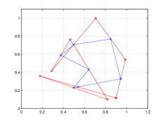
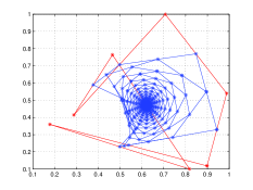
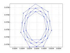
Figure 1: The cyclic pursuit case ($\lambda=1$) with a random initial polygon with $N=7$ points, the first figure presents the initial configuration (in red) and the first iteration (in blue), the second shows the entire evolution for 100 iterations, the last figure displays the scaled up configuration for the last few iterations.

For the general case where $\lambda$ is some real or complex number, we have that

$$\mathbf{P}(t)_{t\rightarrow\infty} = \!\!\!\!\!\left[\begin{array}[]{cccc}1&&&\\ &\lambda^{1/N}&&\\ &&\ddots&\\ &&&\lambda^{\frac{N-1}{N}}\end{array}\right][\mathbf{FT}]\left[\begin{array}[]{cccc}\mu_{0}^{t}&&&\\ &\mu_{1}^{t}&0&\\ &0&\ddots&\\ &&&\mu_{N-1}^{t}\end{array}\right]_{t\rightarrow\infty}\!\!\!\!\!\!\!\!\!\!\widetilde{\mathbf{P}}(0)$$

$$= \!\!\!\!\!\left[\begin{array}[]{cccc}1&&&\\ &\lambda^{1/N}&&\\ &&\ddots&\\ &&&\lambda^{\frac{N-1}{N}}\end{array}\right][\mathbf{FT}]\left[\begin{array}[]{cccc}\mu_{0}^{t}&&&\\ &0&0&\\ &0&\ddots&\\ &&&0\end{array}\right]_{t\rightarrow\infty}\!\!\!\!\!\!\!\!\!\!\widetilde{\mathbf{P}}(0),$$

where $\mu_{0}=\frac{1}{2}(1+\lambda^{1/N})$ is the dominant eigenvalue. Since

$$\widetilde{\mathbf{P}}(0)=[\mathbf{FT}]^{*}\left[\begin{array}[]{cccc}1&&&\\ &\lambda^{-1/N}&&\\ &&\ddots&\\ &&&\lambda^{\frac{-(N-1)}{N}}\end{array}\right]\mathbf{P}(0),$$

we then have that

$$\mathbf{P}(t)_{t\rightarrow\infty}\!\!\!\! = \!\!\!\!\mu_{0}^{t}\left[\begin{array}[]{cccc}1&&&\\ &\lambda^{1/N}&&\\ &&\ddots&\\ &&&\lambda^{\frac{N-1}{N}}\end{array}\right][\mathbf{FT}]_{l,1}([\mathbf{FT}]_{l,1})^{*}\left[\begin{array}[]{cccc}1&&&\\ &\lambda^{-1/N}&&\\ &&\ddots&\\ &&&\lambda^{\frac{-(N-1)}{N}}\end{array}\right]\mathbf{P}(0)$$

and since the first column of the Fourier transform is a vector of all ones, this further simplifies to

$$\mathbf{P}(t)_{t\rightarrow\infty}=\mu_{0}^{t}\frac{1}{N}\left[\begin{array}[]{c}1\\ \lambda^{1/N}\\ \vdots\\ \lambda^{\frac{N-1}{N}}\end{array}\right][1,\lambda^{-1/N},\ldots,\lambda^{\frac{-(N-1)}{N}}]\mathbf{P}(0).$$

Therefore, we see that the limiting behavior is dominated by

$$\mathbf{P}(t)_{t\rightarrow\infty}=\left[\frac{1}{2}(1+\lambda^{1/N})\right]^{t}\frac{1}{N}\underbrace{[1,\lambda^{-1/N},\ldots,\lambda^{\frac{-(N-1)}{N}}]\mathbf{P}(0)}_{\mbox{a (complex) scalar}}\left[\begin{array}[]{c}1\\ \lambda^{1/N}\\ \vdots\\ \lambda^{\frac{N-1}{N}}\end{array}\right].$$

We can distinguish different behaviors depending on $\lambda$.

1. if $\lambda$ is real and $|\lambda|<1$, $\mathbf{P}(t)$ tends to zero, but the limit behavior will be a linear constellation of points

   $$(\alpha_{t})_{x}\left[\begin{array}[]{c}1\\ \lambda^{1/N}\\ \vdots\\ \lambda^{\frac{N-1}{N}}\end{array}\right]+i(\alpha_{t})_{y}\left[\begin{array}[]{c}1\\ \lambda^{1/N}\\ \vdots\\ \lambda^{\frac{N-1}{N}}\end{array}\right].$$

   If $|\lambda|>1$, the constellation of agent locations will diverge in a similar formation.

2. If $\lambda$ is a complex number $\rho_{(\lambda)}e^{i\varphi_{(\lambda)}}$, the convergence/divergence will depend on the angle of rotation induced by $\varphi_{(\lambda)}$ and on the magnitude $\rho_{(\lambda)}$. As seen in the examples provided in Figures 2, 3, 4, 5, 6, 7, in the limit, agents are marching in elliptic or circular arcs, spiralling towards their point of convergence (and in case of divergence, spiralling out to infinity). As in Figure 1, the left figure presents the initial configuration (in red) and the first iteration (in blue), the second shows the entire evolution for 100 iterations (unless stated otherwise), the last figure displays the scaled up configuration for the last few iterations.

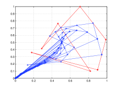
Figure 2: $\lambda=0.1$

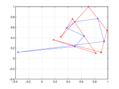
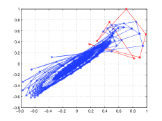
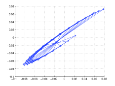
Figure 3: $\lambda=-1$

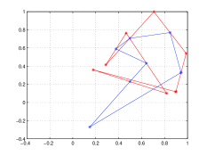
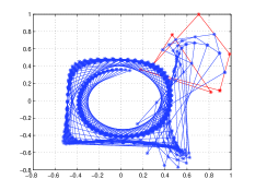
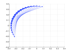
Figure 4: $\lambda=i$

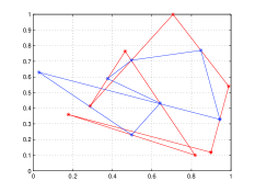
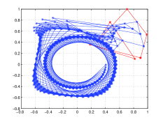
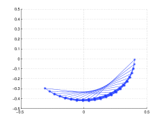
Figure 5: $\lambda=-i$

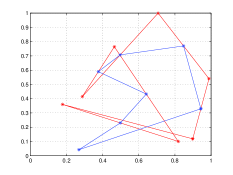
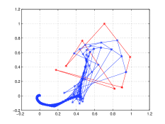
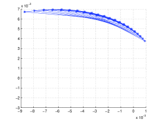
Figure 6: $\lambda=\exp(i\pi/4)/2$

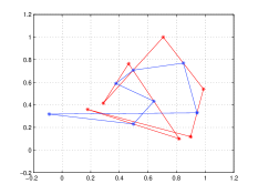
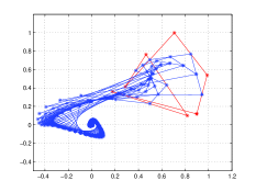
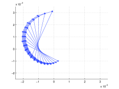
Figure 7: $\lambda=\exp(i\pi/4+i\pi)/2$

4.2 Centroid gathering evolution and extensions

As a second example, suppose that agent $\mathcal{P}_{k}$ is moving according to the following linear combination of its own position, the positions of agents higher in the hierarchy i.e. $\{\mathcal{P}_{k+1},\ldots,\mathcal{P}_{N-1}\}$ and the positions of those lower than itself $\{\mathcal{P}_{0},\mathcal{P}_{1},\ldots,\mathcal{P}_{k-1}\}$:

$$\mathcal{P}_{k}(t+1)=\alpha\mathcal{P}_{k}(t)+\beta_{F}\sum_{l=k+1}^{N-1}\mathcal{P}_{l}(t)+\beta_{B}\sum_{l=0}^{k-1}\mathcal{P}_{l}(t)$$

or

$$\mathbf{P}(t+1)=\left[\begin{array}[]{ccccc}\alpha&\beta_{F}&\beta_{F}&\ldots&\beta_{F}\\ \beta_{B}&\alpha&\beta_{F}&\ldots&\beta_{F}\\ &&\ddots&&\vdots\\ &&&&\\ \beta_{B}&\ldots&\ldots&\beta_{B}&\alpha\end{array}\right]\mathbf{P}(t).$$

Note that if $\beta_{F}=\beta_{B}=(1-\alpha)/(N-1)$, we will have

$$\mathcal{P}_{k}(t+1) = \alpha\mathcal{P}_{k}(t)+\frac{1-\alpha}{N-1}\sum_{l=0,l\neq k}^{N}\mathcal{P}_{l}(t)$$

$$= \frac{N\alpha-1}{N-1}\mathcal{P}_{k}(t)+\left(1-\frac{N\alpha-1}{\alpha-1}\right)\mathcal{P}_{centroid}$$

hence all agents move towards the time-invariant centroid on straight lines.

For general $\beta_{F}$ and $\beta_{B}$, the above matrix is $\beta_{B}/\beta_{F}$-factor circulant and is diagonalized by

$$\mathbf{\widetilde{P}}(t)=[\mathbf{FT}]^{*}\left[\begin{array}[]{cccc}1&&&\\ &(\beta_{B}/\beta_{F})&0&\\ &&\ddots&\\ &0&&(\beta_{B}/\beta_{F})^{N-1}\end{array}\right]\mathbf{P}(t),$$

the modes or eigenvalues being given by

$$\mu_{l}=\alpha+\sum_{k=1}^{N-1}\beta_{F}\left(\frac{\beta_{B}}{\beta_{F}}\right)^{\frac{k}{N}}e^{-i\frac{2\pi}{N}kl},~{}l=0,\ldots,N-1.$$

Let us consider first the case of perfectly cyclic interaction, i.e., when $\beta_{B}=\beta_{F}$. In this case, the interaction matrix is circulant, and we have

$$\mu_{l}=\alpha+\sum_{k=1}^{N-1}\beta_{F}e^{-i\frac{2\pi}{N}kl},~{}l=0,\ldots,N-1$$

and

$$\mu_{0} = \alpha+(N-1)\beta_{F}$$

$$\mu_{l} = \alpha-\beta_{F}+\sum_{k=0}^{N-1}\beta_{F}e^{-i\frac{2\pi}{N}kl}=\alpha-\beta_{F}.$$

For normalization, we shall take $\beta_{F}=(1-\alpha)/(N-1)$ and then

$$\mu_{0} = 1$$

$$\mu_{l} = (N\alpha-1)/(N-1),\mbox{ for all }l.$$

We now have that

$$\widetilde{\mathbf{P}}(t)=[\mathbf{FT}]^{*}\mathbf{P}(t)$$

evolves according to

$$\widetilde{\mathbf{P}}(t)_{t\rightarrow\infty}=\left[\begin{array}[]{cccc}1&&&\\ &\left(\frac{N\alpha-1}{N-1}\right)^{t}&&\\ &&\ddots&\\ &&&\left(\frac{N\alpha-1}{N-1}\right)^{t}\end{array}\right]\widetilde{\mathbf{P}}(0)\\ =\left[\begin{array}[]{c}1\\ 0\\ \vdots\\ 0\end{array}\right][1,0,\ldots,0]\widetilde{\mathbf{P}}(0).$$

Hence

$$\mathbf{P}(t)_{t\rightarrow\infty}=[\mathbf{FT}]\left[\begin{array}[]{c}1\\ 0\\ \vdots\\ 0\end{array}\right][1,0,\ldots,0][\mathbf{FT}]^{*}\mathbf{P}(0)\\ =\frac{1}{N}\left[\begin{array}[]{c}1\\ 1\\ \vdots\\ 1\end{array}\right][1,1,\ldots,1]\mathbf{P}(0)$$

i.e., as we have already seen, all points converge towards the centroid of the initial constellation. The convergence will be as follows:

$$\mathbf{P}^{N}(t)_{t\rightarrow\infty}=\widetilde{\mathbf{P}}(t)-\left[\begin{array}[]{c}1\\ 0\\ \vdots\\ 0\end{array}\right][1,0,\ldots,0]\widetilde{\mathbf{P}}(0)\\ =\left(\frac{N\alpha-1}{N-1}\right)^{t}\left[\begin{array}[]{cccc}0&&&\\ &1&&\\ &&\ddots&\\ 0&&&1\end{array}\right]\widetilde{\mathbf{P}}(0).$$

Therefore

$$\mathbf{P}^{N}(t)_{t\rightarrow\infty} = [\mathbf{FT}]\left(I-\left[\begin{array}[]{c}1\\ 0\\ \vdots\\ 0\end{array}\right][1,0,\ldots,0]\right)[\mathbf{FT}]^{*}\widetilde{\mathbf{P}}(0)$$

$$= \left(\frac{N\alpha-1}{N-1}\right)^{t}\left(\mathbf{P}(0)-\left[\begin{array}[]{c}1\\ 1\\ \vdots\\ 1\end{array}\right][1,1,\ldots,1]\mathbf{P}(0)\right).$$

Consequently, all agents will gather towards the centroid by moving on a line from $\mathcal{P}_{k}(0)$ to $(1/N)\sum_{i=1}^{N-1}\mathcal{P}_{i}(0)$ (see Figure 8).

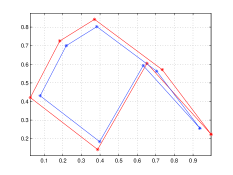
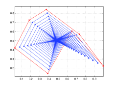
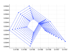
Figure 8: $\lambda=1$, $\alpha=0.1$, 100 iterations

Next suppose we have $\beta_{B}\neq\beta_{F}$. Then we have a $\lambda=\beta_{B}/\beta_{F}$ factor circulant and the modes of the $\widetilde{\mathbf{P}}(t)$ evolution is controlled by

$$\mu_{l}=\alpha+\sum_{k=1}^{N-1}\beta_{F}\left(\frac{\beta_{B}}{\beta_{F}}\right)^{k/N}e^{-i\frac{2\pi}{N}kl},~{}l=0,\ldots,N-1.$$

Here

$$\mu_{0} = \alpha-\beta_{F}+\beta_{F}\sum_{k=0}^{N-1}\left(\frac{\beta_{B}}{\beta_{F}}\right)^{k/N}$$

$$= \alpha-\beta_{F}+\beta_{F}\frac{\beta_{B}/\beta_{F}-1}{(\beta_{B}/\beta_{F})^{1/N}-1}$$

$$= \alpha-\frac{1-\alpha}{N-1}+\left(\frac{1-\alpha}{N-1}\right)\left(\frac{\lambda-1}{\lambda^{1/N}-1}\right).$$

Similarly we have that

$$\mu_{l} = \alpha+\sum_{k=1}^{N-1}\beta_{F}\left(\frac{\beta_{B}}{\beta_{F}}\right)^{k/n}e^{-i\frac{2\pi}{N}kl}$$

$$= \alpha-\frac{1-\alpha}{N-1}+\left(\frac{1-\alpha}{N-1}\right)\left(\frac{\lambda e^{-i\pi l}-1}{\lambda^{1/N}e^{i\pi l/N}-1}\right).$$

In this example too, as before, we have

$$\mathbf{P}(t)_{t\rightarrow\infty}=\left[\begin{array}[]{l}1{}{}{}\\ ~{}~{}~{}\lambda^{1/N}\\ ~{}~{}~{}~{}~{}\ddots\\ 0~{}~{}~{}~{}~{}~{}~{}~{}\lambda^{\frac{N-1}{N}}\end{array}\right][\mathbf{FT}]\left[\begin{array}[]{cccc}\mu_{0}^{t}&&&\\ &\mu_{1}^{t}&&\\ &&\ddots&\\ 0&&&\mu_{N-1}^{t}\end{array}\right][\mathbf{FT}]^{*}\left[\begin{array}[]{l}1\\ ~{}~{}~{}\lambda^{-1/N}\\ ~{}~{}~{}~{}~{}\ddots\\ 0~{}~{}~{}~{}~{}~{}~{}\lambda^{\frac{-(N-1)}{N}}\end{array}\right]{\mathbf{P}}(0)$$

and if $\mu_{0}$ is the dominant eigenvalue, we shall have

$$\mathbf{P}(t)_{t\rightarrow\infty}=\mu_{0}^{t}\frac{1}{N}\left[\begin{array}[]{c}1\\ \lambda^{1/N}\\ \vdots\\ \lambda^{N-1/N}\end{array}\right][1,\lambda^{-1/N},\ldots,\lambda^{-(N-1)/N}]\mathbf{P}(0)$$

and depending on the values selected for $\lambda$, we can get a wealth of interesting behaviors while the solutions converge or diverge to infinity, displaying spiralling or in line marching. See Figures 9, 10, 11, 12, 13, 14 where we present a few interesting cases.

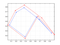
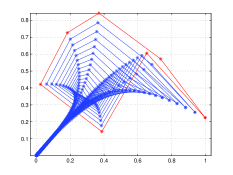
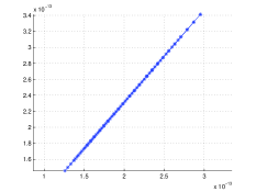
Figure 9: $\lambda=0.5$, $\alpha=0.1$, 1000 iterations

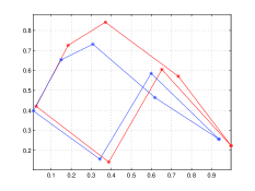
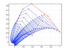
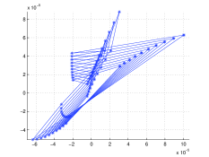
Figure 10: $\lambda=-1$, $\alpha=0.1$, 100 iterations

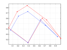
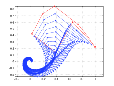
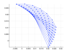
Figure 11: $\lambda=i$, $\alpha=0.1$, 100 iterations

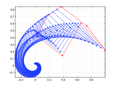
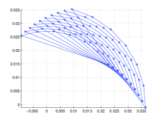
Figure 12: $\lambda=-i$, $\alpha=0.1$, 100 iterations

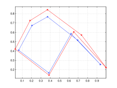
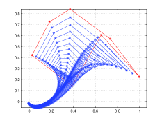
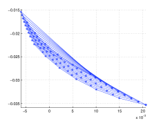
Figure 13: $\lambda=\exp(i\pi/4)/2$, $\alpha=0.1$, 100 iterations

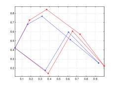
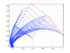
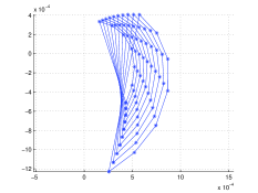
Figure 14: $\lambda=\exp(i\pi/4+i\pi)/2$, $\alpha=0.1$, 100 iterations

5 Concluding Remarks

We discussed in this paper a special type of cyclic multiagent interaction modeled by $\lambda$-factor cyclic matrices. Such matrices allow explicit closed form diagonalizations via generalized Fourier transforms hence enable the analysis of the evolution of the swarm via a nice, geometric, modal decomposition process. It is expected that a wealth of further similar, structured and nearly cyclic interactions will also yield explicit closed form solutions for their asymptotic behavior. In fact, we may use evolutions that fix one, two [16] or several agents in the swarm and use circulant or $\lambda$-circulant interactions for the rest of them leading to further highly structured matrices that can be diagonalized, and correspondingly leading to interesting and explicitly predictable and designable swarm dynamics. In closing, we note that Turing’s morphogenesis may be regarded as a further example of such dynamics for points in the plane where the $x$ and the $y$ coordinates are subjected to different linear circulant transformations also readily generalizable to $\lambda$-circulant maps [15]. An analysis of such swarm interaction for multiagent system is forthcoming.

References

[1]
E.C. Boman.
The Moore Penrose pseudoinverse of an arbitrary, square,
k-circulant matrix.
Linear and Multilinear Algebra, 50:175–179, 2002.
[2]
A.M. Bruckstein, N. Cohen, and A. Efrat.
Ants, crickets and frogs in cyclic pursuit.
CIS9105 technical report, Computer Science Dept., Technion, 1991.
[3]
A.M. Bruckstein, G. Sapiro, and D. Shaked.
Evolutions of planar polygons.
International Journal of Pattern Recognition and Artificial
Intelligence, 9(6):991–1014, 1995.
[4]
R.E. Cline, R.J. Plemmons, and G. Worm.
Generalized inverses of certain Toeplitz matrices.
Linear Algebra and Its Applications, 8:25–33, 1974.
[5]
M. G. Darboux.
Sur un problème de géométrie élémentaire.
Bull. Sci. Math., 2:298–304, 1878.
[6]
P. Elia, F. Oggier, and P. Vijay Kumar.
Asymptotically optimal cooperative wireless networks without
constellation expansion.
IEEE Journal on Selected Areas in Communications on Cooperative
Communications and Networking, 25, 2007.
[7]
P. Feinsilver.
Circulants, inversion of circulants, and some related matrix
algebras.
Linear. Algebra and Appl., 56:29–43, 1984.
[8]
I. Gohberg and V. Olshevsky.
Circulants, displacements and decompositions of matrices.
Integral Equations and Operator Theory, 15:730–743, 1992.
[9]
R.M. Gray.
Toeplitz and circulant matrices: A review.
Intelligent systems lab technical memo, Stanford University,
1971-2006.
[10]
F. Hirsh and S. Smale.
Differential Equations, Dynamical Systems and Linear Algebra.
Academic Press, 1974.
[11]
J.A. Marshall and M.E Broucke.
Symmetry invariance of multiagent formations in self-pursuit.
IEEE Transactions on Automatic Control, 53(9):2022–2032, 2008.
[12]
J.A. Marshall, M.E Broucke, and B.A. Francis.
Formations of vehicles in cyclic pursuit.
IEEE Transactions on Automatic Control, 49(11):1963–1974,
2004.
[13]
I. J. Schoenberg.
The finite Fourier series and elementary geometry.
Amer. Math. Monthly, 57(6):390–404, 1950.
[14]
D. B. Shapiro.
A periodicity problem in plane geometry.
The American Math. Monthly, 91:97–108, 1984.
[15]
A.M. Turing.
The chemical basis of morphogenesis.
Philosophical Transactions of the Royal Society of London,
series B, Biological Sciences, 237(641), 1952.
[16]
I. Wagner and A.M. Bruckstein.
Row straightening by local interactions.
Circuits, Systems and Signal Processing, 16(3):287–305, 1997.
[17]
A.C. Wilde.
Differential equations involving circulant matrices.
Rocky Mount. J. Math., 13(1):1–13, 1983.