Non-perturbative renormalization of bilinear operators with dynamical overlap fermions

Abstract

Using the non-perturbative renormalization technique, we calculate the renormalization factors for quark bilinear operators made of overlap fermions on the lattice. The background gauge field is generated by the JLQCD and TWQCD collaborations including dynamical effects of two or 2+1 flavors of light quarks on a 16${}^{3}\times$32 or 16${}^{3}\times$48 lattice at lattice spacing around 0.1 fm. By reducing the quark mass close to the chiral limit, where the finite volume system enters the so-called $\epsilon$-regime, the unwanted effect of spontaneous chiral symmetry breaking on the renormalization factors is suppressed. On the lattices in the conventional $p$-regime, this effect is precisely subtracted by separately calculating the contributions from the chiral condensate.

I Introduction

For lattice calculations of operator matrix elements including those of electroweak effective Hamiltonian, the operator matching is a necessary step to absorb the difference of the renormalization scheme from the conventional continuum one, such as the $\overline{\mathrm{MS}}$ scheme. This is necessary for most composite operators except for those protected by some symmetry, e.g. the conserved vector current, since the operators are defined with a given lattice action and in general divergent in the continuum limit. This operator matching can be done perturbatively and has been done often at the one-loop level, which induces a potential source of large systematic error. Given that the strong coupling constant $\alpha_{s}$ is in the range 0.2–0.3, a typical size of the two-loop correction is 4–10%. Non-perturbative technique to calculate this operator matching is therefore highly desirable to achieve precise calculation of physical quantities.

The Non-Perturbative Renormalization (NPR) method uses the RI/MOM scheme Martinelli et al. (1995) in an intermediate step. This scheme is defined for the amputated Green’s function in the Landau-gauge with an off-shell momentum, which is space-like. Since the matching between the RI/MOM and the $\overline{\mathrm{MS}}$ schemes are known to two-loop order in many important operators, the method provides a better matching scheme as a whole, though not the entire steps are non-perturbative. Moreover, since the perturbative series is in general more convergent in the continuum schemes, the remaining uncertainty can be made small to a few percent level.

Since the method still requires perturbative expansion, the renormalization condition has to be applied in the region where non-perturbative effects are sufficiently small. On the other hand, one has to avoid large discretization effects that may arise when the renormalization scale is too high. Therefore, the renormalization scale $\mu$ must satisfy the condition $\Lambda_{QCD}\ll\mu\ll\pi/a$, where $\Lambda_{QCD}$ stands for the QCD scale and $a$ is the lattice spacing. This region is often called the NPR window.

The non-perturbative effect may be enhanced when the spontaneous chiral symmetry breaking (SCSB) occurs and (almost) massless pions arise Martinelli et al. (1995). The reason is that the pion-pole contribution in the pseudoscalar channel diverges towards the massless limit and makes it difficult to find the NPR window. With the Wilson-type fermions, the problem is severer because the error starts at ${\cal O}(a)$ and thus the possible window is narrower in the high momentum regime. Even with the on-shell ${\cal O}(a)$-improved Wilson fermion, the problem remains since the off-shell amplitude is considered in NPR. With the chirally symmetric lattice actions, such as the domain-wall and overlap fermion formulations, the problem becomes more tractable because the ${\cal O}(a)$ error is absent even in off-shell amplitudes.

So far, there have been a number of works that calculate the non-perturbative renormalization factors with the RI/MOM scheme for the domain-wall Blum et al. (2002); Aoki et al. (2008a) and for the quenched overlap fermions DeGrand and Liu (2005); Zhang et al. (2005); Galletly et al. (2007).

In this work, we study the non-perturbative renormalization factors with the RI/MOM scheme for the quark bilinear operators in unquenched QCD with overlap fermions. Our motivation is two-fold. The first is to provide the renormalization factors corresponding to the two-flavor Aoki et al. (2008b) and 2+1-flavor Hashimoto et al. (2007); Matsufuru et al. (2008) gauge configurations generated in the large-scale dynamical overlap project by the JLQCD and TWQCD collaborations, including the quark mass renormalization factor $Z_{m}$ that has been already used in a series of publications Fukaya et al. (2007a, b, 2008); Aoki et al. (2008c); Chiu et al. (2009); Noaki et al. (2008a, b). The second is to study the pion-pole contribution appearing in the NPR calculation in detail and demonstrate a method to control the pion-pole effect in a reliable manner.

Since the low-lying eigenmodes of the Dirac operator are expected to dominate the pion-pole contribution, it is possible to trace its effect as a function of quark mass by explicitly constructing the relevant piece from the low-mode eigenvalues. To be explicit, the pion-pole contribution of the form $\langle\bar{q}q\rangle/p^{2}$ in the operator product expansion contains the chiral condensate $\langle\bar{q}q\rangle$, which is finite in the vacuum of spontaneously broken chiral symmetry. On the lattice of finite volume $V$, it quickly vanishes as quark mass becomes smaller than $\sim 1/\Sigma V$, where $\Sigma$ is the chiral condensate in the infinite volume limit. We identify this term by explicitly comparing the lattice data of the (inverse) quark propagator with the condensate $\langle\bar{q}q\rangle$ constructed from the eigenvalues. Thus, this unnecessary term for NPR can be identified and subtracted. It means that the pion-pole contribution is no longer a problem for the NPR calculation. Clearly, this is possible only when the chiral symmetry is preserved on the lattice. Otherwise, the chiral condensate has a bad cubic divergence even in the massless limit, hence the identification of its physical contribution is not feasible.

This paper is organized as follows. We describe the profile of the gauge configurations used in this work in Section II. In Section III, we discuss the NPR method and its relation to spontaneous chiral symmetry breaking and present our analysis. Results of the calculation are given in Section III.4, where we summarize all results of the renormalization factor available from simple bilinear operators, namely those for the quark mass, the scalar current, the tensor operator and the quark field. (The vector and axial vector currents are treated independently.) Our conclusion is given in Section IV.

II GAUGE CONFIGURATIONS

In order to make this paper self-contained, we briefly describe the generation of the gauge configurations used in this work. We refer Aoki et al. (2008b); Hashimoto et al. (2007); Matsufuru et al. (2008) for more complete description.

We use the overlap fermion formulation Neuberger (1998a, b) on the lattice for both sea and valence quarks. The massless overlap-Dirac operator is defined as

$$D_{\rm ov}(0) = m_{0}\left(1+\gamma_{5}\cdot{\rm sgn}\left[H_{W}(-m_{0})\right]\right),$$ (II.1)

where $H_{W}(-m_{0})\equiv\gamma_{5}D_{W}(-m_{0})$ is the hermitian Wilson-Dirac operator with a large negative mass $-m_{0}$. The massive operator with a bare mass $m$ is constructed from this as

$$D_{\rm ov}(m) = \left(1-\frac{m}{2m_{0}}\right)D_{\rm ov}(0)+m.$$ (II.2)

We use the Hybrid Monte Carlo (HMC) algorithm Duane et al. (1987) to incorporate the fermionic determinant $\det[D_{\rm ov}(m_{\rm sea})]$ (for each flavor) in the path integral.

Since the overlap-Dirac operator contains the sign function, the corresponding determinant changes discontinuously on the border of the global topological charge of the gauge field configuration, which makes the simulation time-consuming. In order to avoid touching the border, where the sign of the lowest eigenvalue of $H_{W}$ changes, we introduce two extra flavors of heavy Wilson fermions such that they produce a factor

$$\det\left[\frac{H_{\rm W}^{2}(-m_{0})}{H_{\rm W}^{2}(-m_{0})+\mu^{2}}\right]$$ (II.3)

in the Boltzmann weight. Associated (twisted-mass) bosons are also introduced with a twisted mass $\mu$. They play a role to minimize the change of the effective gauge coupling induced by those extra fermions. Throughout this paper, we choose $m_{0}=1.60$ and $\mu=0.20$ in the lattice unit. As a result, the topological charge $Q$ of the generated gauge configurations is fixed to its initial value Fukaya et al. (2006). In this work, we choose $Q=0$. Although the correct sampling of the $\theta$-vacuum of QCD is spoiled due to the fixed topology, the difference is suppressed for large four-volume $V$, and it is indeed possible to reconstruct the $\theta$-vacuum physics from those evaluated by the path integral in a fixed topology Aoki et al. (2007). In any case, such finite volume effects are irrelevant for the calculation of the renormalization constants considered in this work, as it mainly uses the high momentum regime.

ensemble	NF2$\epsilon$	NF2p	NF3p-a	NF3p-b
$N_{f}$	2	2	2+1
$\beta$	2.35	2.30	2.30
$a^{-1}$ [GeV]	1.776(38)	1.667(17)	1.833(12)
lattice size	$16^{3}\times 32$	$16^{3}\times 32$	$16^{3}\times 48$
$m_{\rm sea}$ ($m_{ud}$)	0.002	0.015, 0.025, 0.035, 0.050, 0.070, 0.100	0.015, 0.025, 0.035, 0.050, 0.080	0.015, 0.025, 0.035, 0.050, 0.100
$m_{s}$	$\infty$	$\infty$	0.080	0.100
$m_{q}$	0.002, 0.015, 0.025, 0.035, 0.050, 0.070, 0.100	0.015, 0.025, 0.035, 0.050, 0.070, 0.100	0.015, 0.025, 0.035, 0.050, 0.080	0.015, 0.025, 0.035, 0.050, 0.100
#trajectories	2,000	10,000	2,500	2,500
#step traj. (NPR)	10	100	10
#step traj. (WTI)	see text	20	5
#low-modes	$50\times 2$	$50\times 2$	$80\times 2$
# of $p_{\rm latt}$ ($(p_{\rm latt})^{2}$)	1,375 (30)	1,375 (30)	1,875 (53)
Relevant papers	Fukaya et al. (2007a, b, 2008)	Aoki et al. (2008c); Noaki et al. (2008a); Shintani et al. (2009)	Noaki et al. (2008b)

Table 1: Parameter set for each gauge ensemble NF2$\epsilon$, NF2p, NF3p-a and NF3p-b. Number of trajectories are common for all sea quark masses in each ensemble.

In Table 1, we list the parameter set for each gauge ensemble on which we calculate the renormalization factors in this work. We performed two-flavor ($N_{f}=2$) and 2+1-flavor ($N_{f}=2+1$) runs. One of the simulations “NF2$\epsilon$” is in the so-called $\epsilon$-regime of the chiral perturbation theory, which corresponds to a very small sea quark mass so that the pion’s Compton wave length is longer than the lattice extent. The sea quark mass $m_{\rm sea}$ = 0.002 roughly corresponds to 3 MeV in the physical unit. Other runs at $N_{f}=2$, “NF2p”, are in the conventional $p$-regime, where we take six values of $m_{\rm sea}$. The 2+1-flavor runs are performed at two different values of the strange quark mass, $m_{s}$ = 0.080 (“NF3p-a”) and 0.100 (“NF3p-b”), so that we can interpolate (or extrapolate) the data to the physical strange quark mass afterwards. For each $m_{s}$, we take five values of sea quark mass corresponding to the up and down quarks $m_{ud}$.

We employ the Iwasaki gauge action for the gauge part of the lattice formulation. The parameter $\beta$ in the action controls the lattice spacing $a$; we determine the value of the lattice spacing from the Sommer scale $r_{0}$ by taking $r_{0}$ = 0.49 fm as an input after extrapolating the lattice data to the chiral limit $m_{\rm sea}=0$ or $m_{ud}=0$ at a fixed $\beta$. The spatial lattice size is $16^{3}$ and the temporal size is 32 and 48 for the two-flavor and the 2+1-flavor runs, respectively.

The valence quark propagator on each ensemble is computed using the multi-shift solver at various valence quark masses. For each ensemble in the $p$-regime, we take the same set of masses for the valence quark as that for the sea quarks as listed in Table 1. For NF2$\epsilon$, we take seven values of valence quark mass: $m_{q}$ = 0.002, 0.025, 0.015, 0.035, 0.050, 0.070, and 0.100.

On each gauge configuration fixed to the Landau gauge, we compute the quark propagator $S_{\rm ov}(x|x_{\rm src})\equiv[D_{ov}(m_{q})^{-1}]_{x,x_{\rm src}}$, where the location of the source $x_{\rm src}$ is typically fixed at the origin. To calculate the renormalization factors, we work in the (four-dimensional) momentum space,

$$S_{\rm ov}(p_{\rm latt})=\sum_{x}e^{-ip_{\rm latt}\cdot x}S_{\rm ov}(x|x_{\rm src}).$$ (II.4)

To avoid possible large discretization error, we restrict the lattice momentum $p_{\rm latt}$ such that its each element $p_{\rm latt}^{\mu}=2\pi n_{\mu}/L_{\mu}$ does not exceed unity. The numbers of lattice momenta satisfying this condition are listed in Table 1. Some of them are degenerate in their magnitude $(p_{\rm latt})^{2}$; the number of available data point in $(p_{\rm latt})^{2}$ is also listed in parentheses. On a $16^{3}\times 32$ lattice, for instance, we have 1,375 different four-momentum from the condition $-2\leq n_{i}\leq 2\ (i=1,2,3)$ and $-5\leq n_{4}\leq 5$, and there are 30 different values of $(p_{\rm latt})^{2}$. When analyzing the lattice data, we first average over different four-momenta giving an identical $(p_{\rm latt})^{2}$.

III RI/MOM renormalization on the lattice

III.1 Renormalization condition and axial-Ward-Takahashi Identity

We consider flavor non-singlet bilinear operators of the form $\bar{q}\Gamma q^{\prime}$ with $\Gamma$ = $\gamma_{\mu}$, $\gamma_{\mu}\gamma_{5}$, $I$, $\gamma_{5}$ and $\gamma_{\mu}\gamma_{\nu}$, that we call $V$, $A$, $S$, $P$ and $T$, respectively. In the following, we may omit the prime in $q^{\prime}$ that indicates that the quark flavor is different from $q$, but the flavor non-singlet operator is always assumed.

With the exact chiral symmetry of the overlap fermion, these operators are multiplicatively renormalized as

$$(\bar{q}\Gamma q)^{R}(\mu)=Z_{\Gamma}(\mu a)(\bar{q}\Gamma q)^{0},$$ (III.5)

where superscripts $R$ and $0$ represent the renormalized and bare operators, respectively. For divergent operators $S$, $P$ and $T$, the renormalized operator may have a dependence on the renormalization scale $\mu$. The multiplicative renormalization factor $Z_{\Gamma}(\mu a)$ then depends on the scale $\mu$, too. For the vector and axial-vector currents, the renormalization scale dependence is absent because of the current conservation. In the following notation, we may drop the dependence on $\mu$, assuming it implicitly. The quark field $q$ is renormalized as $q^{R}=Z_{q}^{1/2}(\mu a)q^{0}$.

In the RI/MOM scheme Martinelli et al. (1995), the renormalization condition is imposed on the amputated Green’s function $\Lambda_{\Gamma}(p)=\frac{1}{12}\mathrm{Tr}[\left\langle S(p)\right\rangle^{-1}G_{\Gamma}(p)\left\langle S(p)\right\rangle^{-1}\Gamma]$ to satisfy

$$\Lambda_{\Gamma}^{R}(p)=Z_{q}^{-1}(\mu)Z_{\Gamma}\Lambda_{\Gamma}^{0}(p)=1$$ (III.6)

at a space-like off-shell momentum $p^{2}=\mu^{2}$ in the chiral limit. Here, the Green’s function $G_{\Gamma}(p)=\langle q(p)|\bar{q}\Gamma q^{\prime}|\bar{q}^{\prime}(p)\rangle$ is amputated by the vacuum expectation value of the quark propagator $\left\langle S(p)\right\rangle$ and projected with an appropriate gamma matrix $\Gamma$. (The ‘Tr’ denotes the trace over the color and spinor indices.) The RI/MOM scheme is defined for the momentum configuration that the in-coming and out-going quark momenta are the same $p$. Since the definition involves the external quark field, which is not gauge invariant, the renormalization condition depends on the gauge. In the RI/MOM scheme, the Landau gauge is chosen.

In the RI/MOM scheme, the wave function renormalization $Z_{q}$ is fixed by imposing the condition

$$\frac{1}{12i}\mathrm{Tr}\left[\frac{\partial\left\langle S^{R}(p)\right\rangle^{-1}}{\partial p\kern-4.30554pt/}\right]=Z_{q}^{-1}\frac{1}{12i}\mathrm{Tr}\left[\frac{\partial\left\langle S(p)\right\rangle^{-1}}{\partial p\kern-4.30554pt/}\right]=1$$ (III.7)

at $p^{2}=\mu^{2}$ in the chiral limit. Numerically, though, this is not straightforward since it involves a numerical derivative in terms of $p_{\mu}$. Instead, we obtain $Z_{q}$ using (III.6) for the axial-vector vertex function $\Lambda_{A}(p)$ with an input of $Z_{A}$ obtained through the axial-Ward-Takahashi identity

$$Z_{A}^{\rm WTI}\Delta_{4}\langle A_{4}(x){\cal O}(0)\rangle=2m_{q}\langle P(x){\cal O}(0)\rangle,$$ (III.8)

where $A_{4}$ and $P$ are the axial-vector current in the time direction and pseudo-scalar density, respectively. $\Delta_{4}$ denotes the symmetrized difference. This relation must be satisfied as far as the position $x$ of the operator is not too close to the origin, where some interpolating field ${\cal O}$ is set. Once $Z_{A}$ is fixed from this relation, the wave function renormalization is determined as $Z_{q}^{R}(\mu)=Z_{A}^{\rm WTI}\Lambda_{A}(p)$ at $p^{2}=\mu^{2}$.

NF2p		NF3p-a		NF3p-b
$m_{\rm sea}$	$Z_{A}^{\rm WTI}$	$m_{ud}$	$Z_{A}^{\rm WTI}$	$m_{ud}$	$Z_{A}^{\rm WTI}$
0.015	1.37867(61)	0.015	1.38934(49)	0.015	1.38968(47)
0.025	1.37703(45)	0.025	1.38709(40)	0.025	1.38700(36)
0.035	1.37412(40)	0.035	1.38431(32)	0.035	1.38408(32)
0.050	1.37032(33)	0.050	1.38031(27)	0.050	1.38019(31)
0.070	1.36441(31)	0.080	1.37196(21)	0.100	1.36658(26)
0.100	1.35436(29)
0.00	1.38222(82)	“chiral limit”: 1.39360(48)
($\chi^{2}/$dof =	0.43		0.16)

Table 2: Summary of the results of $Z_{A}^{\rm WTI}$ as a function of $m_{\rm sea}$ or $m_{ud}$ for NF2p, NF3p-a and NF3p-b. The last two rows show the results of the extrapolation to the chiral limit as described in the text.

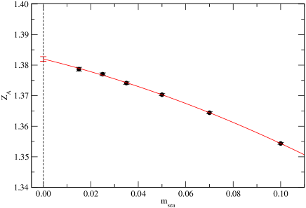
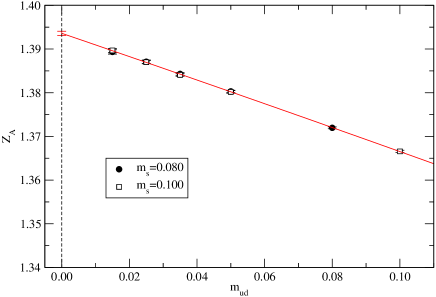
Figure 1: Chiral extrapolation of $Z_{A}^{\rm WTI}$ for NF2p (left panel) and NF3p-a and NF3p-b (right panel).

In practice, we use a pseudo-scalar density with a smeared operator for ${\cal O}$ and sum over spatial lattice sites. Then, we fit a ratio $2m_{q}\sum_{\vec{x}}\langle P(\vec{x},t){\cal O}(0)\rangle/\Delta_{t}\sum_{\vec{x}}\langle A_{4}(\vec{x},t){\cal O}(0)\rangle$ with time slices $t\geq t_{0}$, which is large enough to obtain a constant $Z_{A}^{\rm WTI}$. For NF2$\epsilon$, setting $m_{q}=m_{\rm sea}=0.002$ and $t_{0}=4$, we obtain

$$Z_{A}^{\rm WTI}=1.3511(12).$$ (III.9)

In other ensembles, $Z_{A}^{\rm WTI}$ is obtained for each sea quark mass with the valence quark mass equal to the sea (up and down) quark mass. Results with $t_{0}=7$ for all ensembles are summarized in Table 2, where the second row from the last lists the values extrapolated to the chiral limit. In the chiral extrapolation, we assume linear plus quadratic dependence on $m_{q}$. Since the local axial-vector current we use on the lattice is not a conserved current at finite lattice spacings, the Ward-Takahashi identity (III.8) may be slightly violated. To be explicit, a discretization effect of the form $a^{2}m_{q}\partial_{\mu}P$ is possible as an additive correction to $A_{\mu}$, which leads to the linear dependence on $m_{q}$. Including possible quadratic quark mass dependence, we use

$$Z_{A}^{\rm WTI}(m_{q}) = Z_{A}^{\rm WTI}(0)+C_{1}m_{q}+C_{2}m_{q}^{2}.$$ (III.10)

by setting the valence quark mass as $m_{q}=m_{\rm sea}$ for NF2p and as $m_{q}=m_{ud}$ for the combined data of NF3p-a and NF3p-b. For the case of $N_{f}=2+1$, we assume independence of $Z_{A}$ on $m_{s}$, which appears only as a sea quark. This assumption is indeed supported by the lattice data at two different $m_{s}$.

The vertex function $\Lambda_{\Gamma}(p)$ is calculated on the lattice at many different momentum values $p_{\rm latt}$, whose number is listed in Table 1. With the overlap fermion, we compute the vertex functions as

$$\Lambda_{\Gamma}(p_{\rm latt})=\frac{1}{12}{\rm Tr}\left[\langle\hat{S}_{\rm ov}(p_{\rm latt})\rangle^{-1}\left\langle\hat{S}_{\rm ov}(p_{\rm latt})\Gamma\gamma_{5}\hat{S}_{\rm ov}^{\dagger}(p_{\rm latt})\gamma_{5}\right\rangle\langle\gamma_{5}\hat{S}_{\rm ov}^{\dagger}(p_{\rm latt})\gamma_{5}\rangle^{-1}\Gamma\right]$$ (III.11)

where the quark propagator is effectively given as

$$\hat{S}_{\rm ov}(p)=\frac{2m_{0}}{2m_{0}-m_{q}}\left(S_{\rm ov}(p)-\frac{e^{-ip\cdot x_{\rm src}}}{2m_{0}}\right).$$ (III.12)

This modification of the quark propagator from $S_{\rm ov}(p)$, the inverse of the overlap operator $D_{\rm ov}(m_{q})$, is made in order to incorporate the quark field rotation $q\to(1-\tfrac{D_{\rm ov}(0)}{2m_{0}})q$, $\bar{q}\to\bar{q}$, which is necessary to remove the ${\cal O}(a)$ effects from off-shell quantities. In (III.11), we note that $\gamma_{5}\hat{S}_{\rm ov}^{\dagger}(p_{\rm latt})\gamma_{5}$ cannot be simply replaced by $\hat{S}_{\rm ov}(p_{\rm latt})$ since the l.h.s of (II.4) still depends on the source point $x_{\rm src}$.

III.2 Vector and axial-vector vertex functions

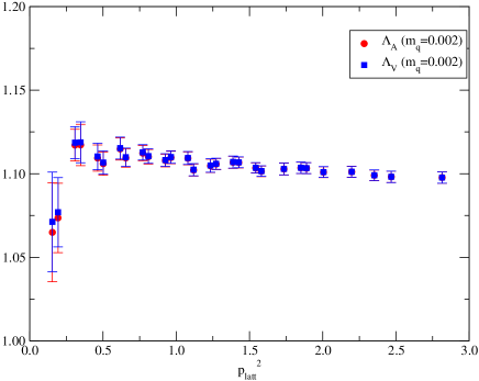
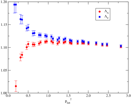
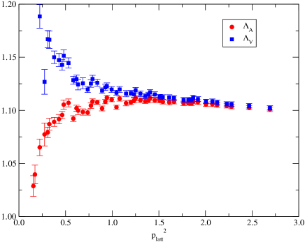
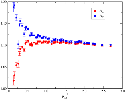
Figure 2: Vertex functions $\Lambda^{\rm latt}_{A}(p_{\rm latt})$ (circles) and $\Lambda^{\rm latt}_{V}(p_{\rm latt})$ (squares) at $m_{q}=0.002$ for NF2$\epsilon$ (upper left) and those in the limit of massless valence quark ($m_{q}=0$) with the sea quark mass fixed at $m_{\rm sea}(m_{ud})=0.015$ for NF2p (upper right), NF3p-a (lower left) and NF3p-b (lower right).

Results for the vector and axial-vector vertex functions are shown in Figure 2 as a function of $p_{\rm latt}^{2}\equiv(\mu a)^{2}$. In the figure, panels from NF2p, NF3p-a and NF3p-b show the data from the lightest $m_{\rm sea}$ or $m_{ud}$. The chiral symmetry implies that these two functions become identical in the massless limit unless the symmetry is spontaneously broken. With exact chiral symmetry of the overlap fermion, this should be the case even at finite lattice spacings. The result in the $\epsilon$-regime (NF2$\epsilon$, upper-left in the figure) clearly shows this behavior, which is consistent with the absence of spontaneous symmetry breaking on a finite volume lattice.

Other three panels, that are obtained in the $p$-regime, show the splitting between the vector and the axial-vector channels. The numerical data in these plots are naively extrapolated to the chiral limit of the valence quarks by assuming a linear dependence on $m_{q}$, but the qualitative picture remains unchanged for each valence quark mass.

This inconsistency among the vector and axial-vector currents may be explained as an effect of the spontaneously broken chiral symmetry. Even on a finite volume lattice, the spontaneous symmetry breaking induces non-zero value of the chiral condensate $-\langle\bar{q}q\rangle\equiv\Sigma$ as far as the quark mass is much larger than a typical scale $1/\Sigma V$. An Operator Product Expansion (OPE) analysis Aoki et al. (2008a) suggests that there are contributions of the form $\Lambda_{\rm QCD}^{2}/p^{2}$ and $m\Lambda_{\rm QCD}/p^{2}$ to the difference $\Lambda_{A}(p)-\Lambda_{V}(p)$. These contributions are induced when the momentum assignment for the three-point function gives vanishing momentum transfer at the vertex. Namely, when the incoming and outgoing momenta are identical as in the RI/MOM-scheme momentum set-up, which is called the “exceptional momenta”, the higher dimensional terms in OPE like $(\bar{q}q)^{2}/p^{6}$ (with some gamma matrices inserted in the numerator) may lead to a much larger contribution of the form $\langle(\bar{q}q)^{2}\rangle/(\Lambda_{\rm QCD}^{4}p^{2})$, which remains in the chiral limit in contrast to the lower order contributions $m^{2}/p^{2}$ or $m\langle\bar{q}q\rangle/p^{4}$ Aoki et al. (2008a). This problem can be avoided by choosing other momentum configurations, such as the RI/SMOM scheme considered in Sturm et al. (2009).

We do not go into details of this problem. But, since the effect becomes statistically significant only below $p_{\rm latt}^{2}\sim$ 1.0–1.5 for the vector and axial-vector channels, we simply use the region that is not largely affected by this effect in the following analysis.

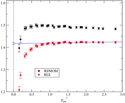
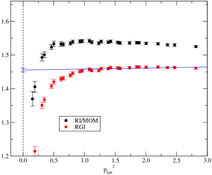
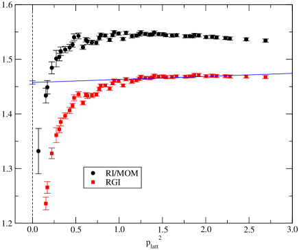
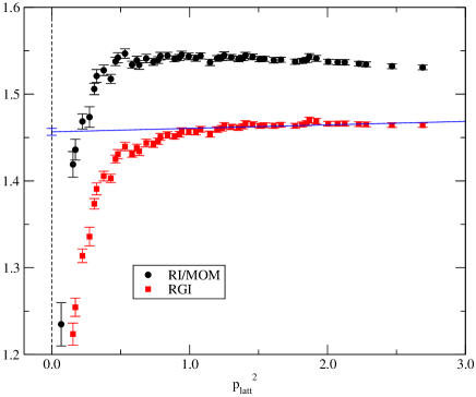
Figure 3: Quark field renormalization factor $Z_{q}$ as a function of $p_{\rm latt}^{2}$. For NF2p, NF3p-a and NF3p-b, data at $m_{\rm sea}(m_{ud})$ = 0.015 are plotted as an example. Results in the RI/MOM scheme are shown by circles, while those in RGI are plotted by squares.

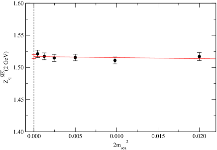
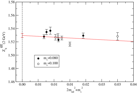
Figure 4: Chiral extrapolation of $Z_{q}^{\overline{\rm MS}}(2\ {\rm GeV})$ on the NF2p (left) and NF3p-a (right, filled symbols) and NF3p-b (right, open symbols) lattices.

$m_{\rm sea}(m_{ud})$	$Z_{q}^{\rm RGI}$	$Z_{q}^{\overline{\rm MS}}(2\ {\rm GeV})$
NF2$\epsilon$, 0.002	1.4170(47)	1.4799(50)
NF2p,  0.015	1.4540(54)	1.5186(56)
0.025	1.4503(51)	1.5147(53)
0.035	1.4479(53)	1.5122(56)
0.050	1.4486(49)	1.5129(51)
0.070	1.4442(51)	1.5083(54)
0.100	1.4500(59)	1.5143(62)
0.000	1.4526(30)	1.5170(31)
($\chi^{2}/$dof	0.33	0.33 )
NF3p-a,  0.015	1.4575(30)	1.5279(31)
0.025	1.4641(38)	1.5348(40)
0.035	1.4660(51)	1.5368(54)
0.050	1.4528(27)	1.5230(29)
0.080	1.4590(37)	1.5294(39)
NF3p-b,  0.015	1.4565(40)	1.5269(42)
0.025	1.4585(32)	1.5290(34)
0.035	1.4555(28)	1.5258(29)
0.050	1.4467(30)	1.5166(31)
0.100	1.4578(55)	1.5283(57)
“chiral limit”:	1.4592(29)	1.5296(31)
($\chi^{2}/$dof	2.20	2.20 )

Table 3: Numerical results for the quark wave function renormalization factor $Z_{q}$. The values in the RGI definition $Z_{q}^{\rm RGI}$ and those defined in the $\overline{\rm MS}$ scheme at $\mu$ = 2 GeV, $Z_{q}^{\overline{\rm MS}}(2{\rm~{}GeV})$ are listed for each sea quark mass.

The quark field renormalization factor $Z_{q}(\mu)$ can be obtained from $\Lambda_{A}(p)$ by multiplying the axial-current renormalization constant $Z_{A}^{\rm WTI}$ as determined from the Ward-Takahashi identity. The results are shown in Figure 3 by filled circles as a function of $p_{\rm latt}^{2}$. The different panels represent the data from the ensembles NF2$\epsilon$, NF2p, NF3p-a, and NF3p-b, respectively. By multiplying the matching factor $1/w_{q}^{\rm RI/MOM}(q)$ at the four-loop level as defined in Appendix A, we may define the Renormalization Group Invariant (RGI) quantity, which is also scheme independent. Our numerical results plotted by squares in Figure 3 clearly show the expected scale independence. Since we expect discretization effects proportional to $a^{2}p_{\rm latt}^{2}$, we fit the lattice data above $(p_{\rm latt})^{2}$ = 1.0 by a linear function and obtain the result for $Z_{q}^{\rm RGI}$ from an intercept at $p_{\rm latt}^{2}=0$. The lattice data below $a^{2}p_{\rm latt}^{2}\simeq$ 1.0 are largely affected by the effect of spontaneously broken chiral symmetry and deviate from the linear behavior as expected.

The results for $Z_{q}^{\rm RGI}$ are listed in Table 3. Also listed are the results converted to the $\overline{\rm MS}$ scheme at $\mu$ = 2 GeV using the four-loop level matching constant $w_{q}^{\overline{\rm MS}}(\mu)$ defined in Appendix A.

So far, the results are given at each sea quark mass after taking the chiral limit of valence quarks. The chiral limit of sea quarks can be taken by assuming that the sea quark mass dependence has the form $Z(1+2c^{(2)}m_{\rm sea}^{2})$ (for NF2p) or $Z(1+c^{(3)}(2m_{ud}^{2}+m_{s}^{2}))$ (for NF3p-a and NF3p-b). The coefficients $c^{(2)}$ and $c^{(3)}$ are numerical constants depending on the number of flavors. The linear term in $m_{\rm sea}$ (or in $m_{ud}$) should not remain for the quantities irrelevant to the chiral symmetry breaking. Figure 4 shows the chiral extrapolation of $Z_{q}^{\overline{\rm MS}}(2\mathrm{~{}GeV})$ for both NF2p and NF3p-a/NF3p-b. We do not observe any significant sea quark mass dependence. The chiral extrapolation should therefore be very stable. The results are listed in Table 3.

III.3 Scalar and Pseudo-scalar vertex functions

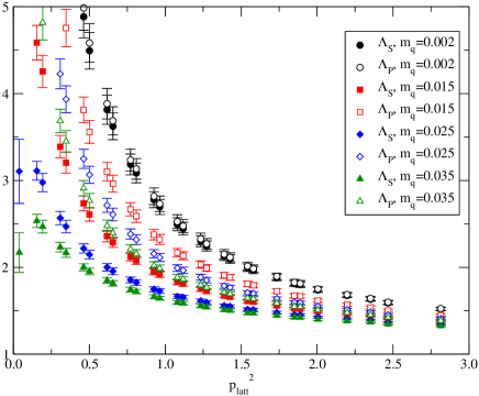
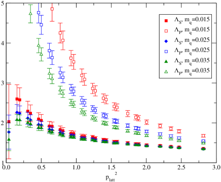
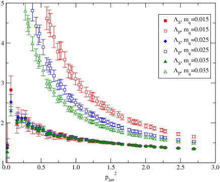
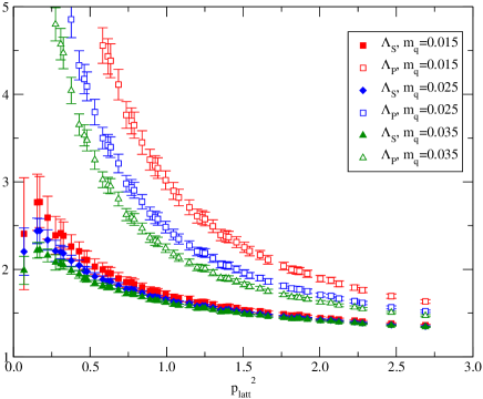
Figure 5: Vertex functions $\Lambda^{\rm latt}_{S}(p_{\rm latt})$ (filled symbols) and $\Lambda^{\rm latt}_{P}(p_{\rm latt})$ (open symbols). The data are shown for NF2$\epsilon$ (upper left), NF2p (upper right), NF3p-a (lower left) and NF3p-b (lower right) as functions of $p_{\rm latt}^{2}$. In each panel, data at $m_{q}=0.015$, $0.025$ and $0.035$ are shown by squares, diamonds and triangles, respectively. For NF2$\epsilon$, data at $m_{q}=0.002$ are shown as well by circles. For NF2p, NF3p-a and NF3p-b, data at the lightest sea quark $m_{\rm sea}(m_{ud})=0.015$ are plotted as an example.

In Figure 5, the momentum dependence of the scalar vertex function $\Lambda_{S}^{\rm latt}(p_{\rm latt})$ (filled symbols) and the pseudo-scalar vertex function $\Lambda_{P}^{\rm latt}(p_{\rm latt})$ (open symbols) is shown for each ensemble. For the data in the $\epsilon$-regime (circles in the upper left panel), we observe an excellent agreement between $\Lambda_{S}(p)$ (filled symbols) and $\Lambda_{P}(p)$ (open symbols), which is expected from the exact chiral symmetry of the overlap fermion. On the other hand, once the valence quark mass $m_{q}$ is out of the $\epsilon$-regime (the data at $m_{q}$ = 0.015, 0.025 and 0.035 are plotted by squares, diamonds and triangles, respectively), we find large disagreement between $\Lambda_{S}(p)$ and $\Lambda_{P}(p)$.

This observation again indicates the effect of the spontaneous chiral symmetry breaking. From the OPE analysis one expects that this effect is more significant than in $\Lambda_{V}(p)$ and $\Lambda_{A}(p)$, because the violation is enhanced by an inverse quark mass as discussed below. One has to subtract this effect in order to extract the renormalization constants because its matching is based on the continuum perturbation theory that does not contain non-perturbative effects.

We consider the quark mass dependence of $\Lambda_{S}(p)$ and $\Lambda_{P}(p)$ using OPE along the line of the analysis in Blum et al. (2002). Using the vector and axial-vector Ward-Takahashi identities, one may obtain relations between the vertex functions and the inverse quark propagators as Giusti and Vladikas (2000)

$$\Lambda_{S}(p) = \frac{1}{12}\frac{\partial\,{\rm Tr}\left\langle S(p)\right\rangle^{-1}}{\partial m_{q}},$$ (III.13)

$$\Lambda_{P}(p) = \frac{1}{12}\frac{{\rm Tr}\left\langle S(p)\right\rangle^{-1}}{m_{q}}.$$ (III.14)

On the lattice we use the improved overlap quark propagator $\hat{S}_{\rm ov}(p)$ in place of $S(p)$. From OPE the inverse quark propagator ${\rm Tr}\left\langle S(p)\right\rangle^{-1}$ may be written as Politzer (1976)

$$\frac{1}{12}{\rm Tr}\left\langle S(p)\right\rangle^{-1}=C\cdot\frac{\left\langle\bar{q}q\right\rangle}{p^{2}}+Z_{q}Z_{m}m_{q}+\cdots$$ (III.15)

in the large $p^{2}$ regime. The effect of the chiral symmetry breaking is picked up through the chiral condensate $\left\langle\bar{q}q\right\rangle$, and $C$ is a perturbatively calculable constant. At the one-loop level, $C=4\pi\alpha_{s}/3$. As in the case of the vector and axial-vector vertex functions, the effects from higher dimensional operators, such as $\langle(\bar{q}q)^{2}\rangle$, may also exist. They are usually suppressed by additional powers of $1/p^{2}$, but due to the lack of the momentum injection the suppression may not work in the case of the inverse quark propagator and of the vertex functions at zero momentum transfer. We therefore leave $C$ as an unknown constant instead of using the perturbatively known value.

Then, using the relations (III.13) and (III.14), we may evaluate the effect of the chiral condensate on the vertex functions as

$$\Lambda_{S}(p) = \frac{C}{p^{2}}\frac{\partial\left\langle\bar{q}q\right\rangle}{\partial m_{q}}+Z_{q}Z_{m}+\cdots,$$ (III.16)

$$\Lambda_{P}(p) = \frac{C}{p^{2}}\frac{\left\langle\bar{q}q\right\rangle}{m_{q}}+Z_{q}Z_{m}+\cdots.$$ (III.17)

From these expressions, one sees an enhancement in the low $p^{2}$ region due to the chiral condensate only for the pseudo-scalar channel, while the scalar channel should not be affected too much because of a derivative with respect to $m_{q}$ rather than a factor $1/m_{q}$.

The quark mass dependence of the condensate $\left\langle\bar{q}q\right\rangle$ is not a trivial issue, since it has effects from both ultraviolet and infrared origins. Since the operator $\bar{q}q$ contains quadratic divergence of the form $m_{q}/a^{2}$ apart from the chiral limit, the chiral condensate $\left\langle\bar{q}q\right\rangle$ directly calculated on the lattice contains unphysical large $m_{q}$ dependence. It has to be subtracted before the analysis using (III.16) and (III.17), because the formulae are obtained as an expansion around the chiral limit.

In the infrared regime, the chiral condensate has a non-trivial quark mass dependence especially in a finite volume. First, because of the pion-loop effects, the chiral condensate develops the chiral logarithm of the form $m_{q}\ln m_{q}$ with known coefficients Gasser and Leutwyler (1984). On a finite volume lattice, the quark mass dependence becomes more complicated. Namely, once the quark mass enters the $\epsilon$-regime, the mass dependence is no longer governed by the simple chiral logarithm, but given by the formula recently developed in Damgaard and Fukaya (2009).

In our analysis, instead of using the formula in Damgaard and Fukaya (2009) we calculate the condensate using its eigenvalue decomposition by making use of the low eigenmodes obtained on the same ensembles. For each lattice configuration, we define

$$(\bar{q}q)^{(N)}=\frac{1}{L_{s}^{3}L_{t}}\sum_{i=1}^{N}\frac{2m_{q}}{m_{q}^{2}+\hat{\lambda}_{i}^{*}\hat{\lambda}_{i}},$$ (III.18)

where $\hat{\lambda}_{i}$ is an eigenvalue of the massless overlap-Dirac operator, which satisfies the eigen equation

$$D_{\rm ov}(0)\left(1-\frac{D_{\rm ov}(0)}{2m_{0}}\right)^{-1}u_{i}(x)=\hat{\lambda}_{i}u_{i}(x)$$ (III.19)

with $u_{i}(x)$ an eigenvector. In (III.18) we use the fact that the eigenvalues appear as complex conjugate pairs. The normalization in (III.18) contains the lattice volume $L_{s}^{3}L_{t}$.

We truncate the sum in (III.18) at $N$-th eigenvalue, which may be considered as a “renormalization scheme” to define the divergent operator $\bar{q}q$. Here, $N$ plays a role of the ultraviolet cut-off. After taking an ensemble average, we denote the chiral condensate thus defined as $\langle\bar{q}q\rangle^{(N)}$. In the course of our project, we calculate and store the low-lying eigenvalues and eigenvectors of the overlap-Dirac operator. In addition to the calculation of the truncated chiral condensate (III.18), these eigenmodes can be used to precondition the solvers, to average over source points, or to construct disconnected diagrams in the calculations of physical observables  Aoki et al. (2008c); Noaki et al. (2008a); Aoki et al. (2009). The numbers of the stored low-modes for each configuration are listed in Table 1.

From a dimensional analysis, the quark mass dependence of $\langle\bar{q}q\rangle^{(N)}$ may be parametrized as

$$\left\langle\bar{q}q\right\rangle^{(N)}=\left\langle\bar{q}q\right\rangle^{\rm(subt)}+c_{1}^{(N)}\frac{m_{q}}{a^{2}}+c_{2}^{(N)}m_{q}^{3}.$$ (III.20)

Because of the exact chiral symmetry of the overlap fermion, there is no leading power divergence of the order $1/a^{3}$, and the term behaves as $m_{q}^{2}/a$ is also absent. Although the cubic term $c_{2}^{(N)}m_{q}^{3}$ in (III.20) may accompany a logarithm $\ln m_{q}$, we omit it for simplicity as the $m_{q}^{3}$ term itself is a minor correction. The subtracted condensate $\langle\bar{q}q\rangle^{\rm(subt)}$ is then free from power divergences, but could still contain non-divergent $m_{q}$ dependence, such as the chiral logarithm.

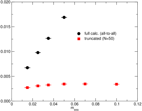
Figure 6: Comparison between $\left\langle\bar{q}q\right\rangle$ obtained from all-to-all propagator (circles) and $\left\langle\bar{q}q\right\rangle^{(N=50)}$ (squares) as a function of $m_{\rm sea}=m_{q}$. The data obtained on NF2p are shown.

In Figure 6, we compare a “full” calculation of $\left\langle\bar{q}{q}\right\rangle$ (circles) corresponding to $N=12L_{s}^{3}L_{t}$ and $\left\langle\bar{q}q\right\rangle^{(N=50)}$. The “full” calculation contains the contributions of all eigenmodes which are evaluated by a stochastic method. (Our set-up is explained in Aoki et al. (2009).) The data on the NF2p lattice with sea and valence quark masses set equal are shown as an example. The results clearly show that the divergent term $m_{q}/a^{2}$ in (III.20) dominates the “full” condensate, and it seems difficult to extract $\langle\bar{q}q\rangle^{\rm(subt)}$ from this data alone. The truncated condensate, on the other hand, does not have that strong $m_{q}$ dependence, but still both the $m_{q}/a^{2}$ and $m_{q}^{3}$ terms are visible.

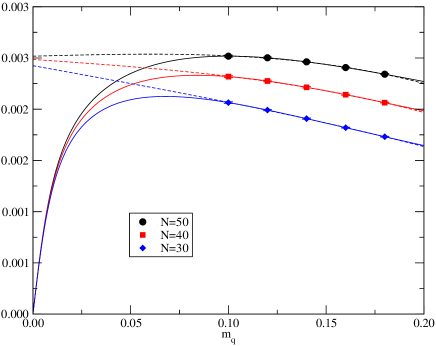
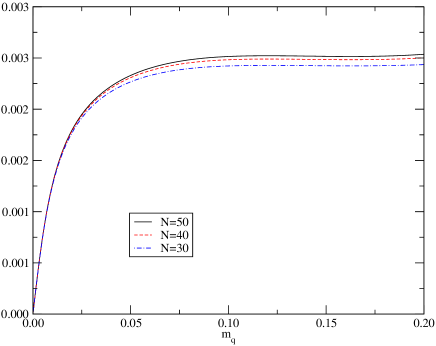
Figure 7: Subtraction of the power divergence in the chiral condensate. The left panel shows $\left\langle\bar{q}q\right\rangle^{(N)}$ calculated on the NF2$\epsilon$ lattice as a function of the valence quark mass $m_{q}$ (solid curves). The number of low-modes included are $N$ = 50, 40 and 30 from top to bottom. The solid curves are data constructed from calculated eigenvalues, and the points with error bars are representative points used in our fit. The fit curves according to (III.20) are shown by dashed curves. The right panel represents the subtracted condensate $\left\langle\bar{q}q\right\rangle^{\rm(subt)}$.

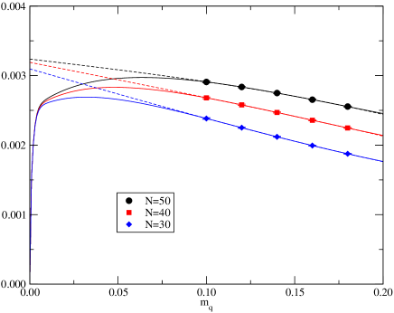
Figure 8: Same as Figure 7 but for NF2p at $m_{\rm sea}=0.015$.

Figure 9: Same as Figure 7 but for NF3p-a (top) and NF3p-b (bottom) at $m_{ud}=0.015$. The number of low-modes included are $N$ = 80, 70, 60 and 50 from top to bottom.

We now try to extract the non-divergent term $\langle\bar{q}q\rangle^{\rm(subt)}$ using (III.20). In Figures 7–9 (left panel) we plot the truncated condensate $\left\langle\bar{q}q\right\rangle^{(N)}$ as a function of the valence quark mass with three or four different values of $N$. The data are shown for individual lattice ensembles (NF2$\epsilon$, NF2p, NF3p-a and NF3p-b); except for NF2$\epsilon$ the results at the lightest sea quark are shown as an example. The truncated condensate can be constructed at arbitrary values of the valence quark mass $m_{q}$ without extra computational costs. In order to see the ultraviolet behavior, we plot in the mass region up to $m_{q}$ = 0.20, which is twice larger than the largest simulated sea quark mass.

When we fit the lattice data to (III.20), we take five or six representative points of $m_{q}$ in the range $0.10\leq m_{q}\leq 0.18$ for NF2$\epsilon$ and NF2p or $0.10\leq m_{q}\leq 0.20$ for NF3p-a and NF3p-b. The upper limit is chosen such that $|\hat{\lambda}_{N}|>m_{q}$ for the given $N$. Otherwise we do not expect the ultraviolet behavior (III.20). In this rather heavy mass region, we do not expect additional mass dependence from the infrared origin, and we simply set $-\left\langle\bar{q}q\right\rangle^{\rm(subt)}=\Sigma$ with $\Sigma$ a constant.

The fit results are shown in Figures 7–9 (left panel) by dashed curves. In each right panel of these figures, the subtracted condensates $\left\langle\bar{q}q\right\rangle^{\rm(subt)}=\left\langle\bar{q}q\right\rangle^{(N)}-c_{1}^{(N)}/a^{2}m_{q}-c_{2}^{(N)}m_{q}^{3}$ for the same choices of $N$ as the left panel are shown. We observe that the subtracted condensate depends on $N$ very mildly to a few % order. It implies that our subsequent analysis using $\left\langle\bar{q}q\right\rangle^{(N)}$ with the maximal $N$ may contain a small systematic error due to the truncation of $N$. We discuss this point and estimate the error in Section III.4.

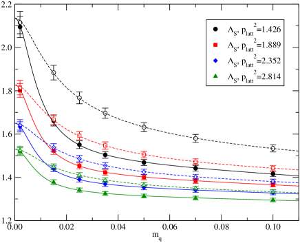
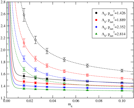
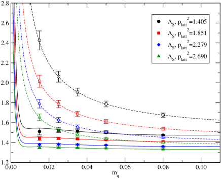
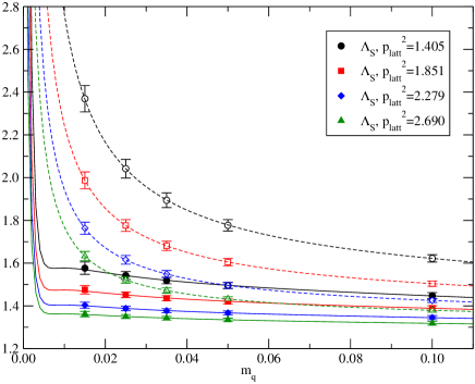
Figure 10: Vertex functions $\Lambda^{\rm latt}_{S}(p_{\rm latt})$ (filled symbols) and $\Lambda^{\rm latt}_{P}(p_{\rm latt})$ (open symbols). The data are shown for the NF2$\epsilon$ (upper left), NF2p (upper right), NF3p-a (lower left) and NF3p-b (lower right) lattices as functions of $m_{q}$. In each panel, data at selected values of $p_{\rm latt}^{2}$ and their fit curves are presented. For NF2p, NF3p-a and NF3p-b, data with a fixed sea quark mass $m_{\rm sea}(m_{ud})=0.015$ are plotted as an example.

We use $\left\langle\bar{q}q\right\rangle^{\rm(subt)}$ thus obtained at each sea quark mass as a function of the valence quark mass in the analysis of the scalar and pseudo-scalar vertex functions, (III.16) and (III.17), respectively. The valence quark mass dependence of $\Lambda^{\rm latt}_{S}(p_{\rm latt})$ and $\Lambda^{\rm latt}_{P}(p_{\rm latt})$ at four representative values of $p_{\rm latt}^{2}$ are plotted in Figure 10. We find that both the scalar (filled symbols) and pseudo-scalar (open symbols) vertices are nicely described by the fit curves according to (III.16) and (III.17) supplemented by the measured $\left\langle\bar{q}q\right\rangle^{\rm(subt)}$. In particular, as seen near the chiral limit of the NF2$\epsilon$ data, the fit curves precisely reproduce the agreement of $\Lambda^{\rm latt}_{S}(p_{\rm latt})$ and $\Lambda^{\rm latt}_{P}(p_{\rm latt})$ in the $\epsilon$-regime, which is not expected when $\left\langle\bar{q}q\right\rangle$ is treated as a mass-independent constant.

In addition to (III.16) and (III.17), quadratic mass-dependence is possible for the vertex functions $\Lambda^{\rm latt}_{S}(p_{\rm latt})$ and $\Lambda^{\rm latt}_{P}(p_{\rm latt})$:

$$\Lambda_{S}(p_{\rm latt}) = \frac{C}{p^{2}}\frac{\partial\left\langle\bar{q}q\right\rangle}{\partial m_{q}}+Z_{q}Z_{m}+B_{S}m_{q}^{2},$$ (III.21)

$$\Lambda_{P}(p_{\rm latt}) = \frac{C}{p^{2}}\frac{\left\langle\bar{q}q\right\rangle}{m_{q}}+Z_{q}Z_{m}+B_{P}m_{q}^{2}.$$ (III.22)

From a combined fit of the valence quark mass dependence, we obtain the parameters $C$, $Z_{q}Z_{m}$, $B_{P}$ and $B_{S}$ at each value of $p_{\rm latt}^{2}$. Numerical results are listed in Tables 4–7 for each sea quark masses of the NF2$\epsilon$, NF2p, NF3p-a and NF3p-b lattices. We find that the values of $C$ depend on $p^{2}$ only mildly, which is consistent with the logarithmic dependence through $\alpha_{s}$.

$p_{\rm latt}^{2}$	$C$	$Z_{q}Z_{m}$	$B_{S}$	$B_{P}$	$\chi^{2}/$dof
1.426	5.92(40)	1.443(16)	$-$3.10(90)	$-$1.35(34)	0.025
1.889	5.01(32)	1.384(13)	$-$2.08(62)	$-$0.85(25)	0.017
2.352	4.32(28)	1.342(11)	$-$1.60(48)	$-$0.76(22)	0.016
2.814	3.78(26)	1.3060(92)	$-$1.23(36)	$-$0.65(15)	0.017

Table 4: Parameters in the simultaneous fit of $\Lambda_{S}^{\rm latt}$ and $\Lambda_{P}^{\rm latt}$ for NF2$\epsilon$. Results at representative values of lattice momenta are listed.

$m_{\rm sea}$	$p_{\rm latt}^{2}$	$C$	$Z_{q}Z_{m}$	$B_{S}$	$B_{P}$	$\chi^{2}/$dof
$0.015$	1.426	8.48(83)	1.472(22)	$-$2.0(1.9)	$-$0.80(91)	0.004
	1.889	7.16(68)	1.412(16)	$-$1.5(1.3)	$-$0.57(66)	0.005
	2.352	6.19(59)	1.366(11)	$-$1.01(95)	$-$0.35(46)	0.005
	2.814	5.31(51)	1.3271(89)	$-$0.65(75)	$-$0.18(38)	0.004
$0.025$	1.426	7.43(39)	1.497(20)	$-$5.3(1.1)	$-$2.21(49)	0.139
	1.889	6.29(32)	1.429(15)	$-$3.53(76)	$-$1.33(35)	0.084
	2.352	5.43(26)	1.380(13)	$-$2.66(56)	$-$1.07(25)	0.071
	2.814	4.61(23)	1.341(10)	$-$2.18(43)	$-$0.96(23)	0.094
$0.035$	1.426	8.57(91)	1.446(24)	$-$0.2(2.0)	$-$0.1(1.1)	0.190
	1.889	7.37(77)	1.392(17)	0.1(1.4)	0.11(71)	0.179
	2.352	6.23(61)	1.353(13)	$-$0.13(92)	$-$0.02(48)	0.133
	2.814	5.40(56)	1.317(11)	0.00(76)	0.09(43)	0.129
$0.050$	1.426	9.00(58)	1.469(21)	$-$1.3(1.5)	$-$0.86(63)	0.021
	1.889	7.61(49)	1.419(15)	$-$1.1(1.1)	$-$0.54(48)	0.014
	2.352	6.54(42)	1.377(12)	$-$0.95(81)	$-$0.59(36)	0.019
	2.814	5.60(37)	1.340(10)	$-$0.89(63)	$-$0.61(31)	0.047
$0.070$	1.426	7.33(54)	1.476(19)	$-$5.1(1.4)	$-$2.19(63)	0.303
	1.889	6.23(45)	1.412(14)	$-$3.56(99)	$-$1.50(45)	0.267
	2.352	5.36(40)	1.363(11)	$-$2.61(78)	$-$1.03(38)	0.228
	2.814	4.56(34)	1.3262(93)	$-$2.23(58)	$-$0.94(30)	0.249
$0.100$	1.426	8.24(61)	1.444(19)	$-$1.9(1.5)	$-$1.09(62)	0.008
	1.889	6.99(53)	1.394(14)	$-$1.4(1.1)	$-$0.81(46)	0.014
	2.352	6.04(47)	1.351(12)	$-$0.92(88)	$-$0.51(42)	0.003
	2.814	5.18(42)	1.316(10)	$-$0.72(74)	$-$0.32(39)	0.004

Table 5: Same as Table 4 but for NF2p.

$m_{ud}$	$p_{\rm latt}^{2}$	$C$	$Z_{q}Z_{m}$	$B_{S}$	$B_{P}$	$\chi^{2}/$dof
$0.015$	1.405	9.00(98)	1.445(21)	2.3(2.8)	1.3(1.5)	0.345
	1.851	7.58(82)	1.393(14)	1.3(1.9)	0.9(1.1)	0.248
	2.279	6.65(72)	1.347(10)	1.2(1.5)	0.87(86)	0.276
	2.690	5.86(62)	1.3228(83)	0.8(1.1)	0.55(58)	0.194
$0.025$	1.405	7.18(52)	1.477(14)	$-$3.5(1.4)	$-$1.59(60)	0.046
	1.851	6.14(44)	1.418(11)	$-$2.77(94)	$-$1.41(42)	0.056
	2.279	5.25(37)	1.3661(93)	$-$2.07(72)	$-$1.03(35)	0.046
	2.690	4.64(32)	1.3379(78)	$-$1.86(53)	$-$0.92(26)	0.065
$0.035$	1.405	7.21(54)	1.495(19)	$-$3.3(2.0)	$-$1.90(81)	0.018
	1.851	6.19(46)	1.427(15)	$-$2.1(1.5)	$-$1.17(58)	0.018
	2.279	5.36(40)	1.376(12)	$-$1.6(1.1)	$-$0.91(48)	0.015
	2.690	4.75(36)	1.3448(97)	$-$1.20(88)	$-$0.58(38)	0.010
$0.050$	1.405	7.88(56)	1.444(16)	$-$0.2(1.9)	$-$0.34(82)	0.098
	1.851	6.80(52)	1.391(12)	0.0(1.5)	$-$0.03(72)	0.099
	2.279	5.82(44)	1.3464(92)	0.0(1.1)	0.14(52)	0.086
	2.690	5.27(43)	1.3216(80)	0.08(98)	0.10(48)	0.075
$0.080$	1.405	9.24(67)	1.449(19)	$-$0.7(2.6)	$-$9.35(78)	0.211
	1.851	8.00(59)	1.395(13)	$-$0.2(1.9)	$-$5.81(59)	0.226
	2.279	6.81(50)	1.352(10)	$-$0.1(1.4)	$-$3.93(47)	0.189
	2.690	6.06(44)	1.3296(86)	$-$0.2(1.1)	$-$3.01(38)	0.138

Table 6: Same as Table 4 but for NF3p-a.

$m_{ud}$	$p_{\rm latt}^{2}$	$C$	$Z_{q}Z_{m}$	$B_{S}$	$B_{P}$	$\chi^{2}/$dof
$0.015$	1.405	8.08(59)	1.464(13)	$-$2.30(94)	$-$0.99(55)	0.020
	1.851	6.92(49)	1.4009(98)	$-$1.57(63)	$-$0.57(35)	0.029
	2.279	5.97(42)	1.3527(78)	$-$1.04(50)	$-$0.34(29)	0.010
	2.690	5.30(37)	1.3239(68)	$-$0.76(41)	$-$0.19(22)	0.007
$0.025$	1.405	7.04(42)	1.4699(93)	$-$2.61(78)	$-$1.21(42)	0.012
	1.851	6.01(36)	1.4101(75)	$-$1.88(56)	$-$0.83(31)	0.004
	2.279	5.19(32)	1.3595(60)	$-$1.34(43)	$-$0.54(22)	0.003
	2.690	4.65(29)	1.3321(52)	$-$1.11(34)	$-$0.51(18)	0.005
$0.035$	1.405	7.14(50)	1.475(11)	$-$3.44(78)	$-$1.39(43)	0.146
	1.851	6.09(41)	1.4126(85)	$-$2.47(54)	$-$1.07(27)	0.087
	2.279	5.26(35)	1.3624(68)	$-$1.84(41)	$-$0.77(22)	0.095
	2.690	4.67(31)	1.3320(58)	$-$1.31(32)	$-$0.48(18)	0.059
$0.050$	1.405	8.93(56)	1.423(15)	$-$0.1(1.3)	0.03(55)	0.295
	1.851	7.59(47)	1.3755(99)	$-$0.09(84)	0.03(37)	0.325
	2.279	6.52(41)	1.3363(77)	$-$0.16(63)	$-$0.01(29)	0.200
	2.690	5.85(36)	1.3115(65)	$-$0.04(50)	0.02(22)	0.240
$0.100$	1.405	8.68(56)	1.468(16)	$-$1.7(1.2)	$-$0.61(60)	0.123
	1.851	7.34(48)	1.412(12)	$-$1.21(91)	$-$0.49(46)	0.113
	2.279	6.26(40)	1.3650(87)	$-$1.00(66)	$-$0.41(29)	0.072
	2.690	5.61(35)	1.3353(75)	$-$0.59(54)	$-$0.24(26)	0.104

Table 7: Same as Table 4 but for NF3p-b.

III.4 Renormalization constants

From the fits described in the previous subsections, we obtain the numerical results for $Z_{q}$ and $Z_{q}Z_{m}=Z_{q}/Z_{S}$ for each available values of $p_{\rm latt}$. From a similar analysis, we also obtain $\Lambda_{T}=Z_{q}Z_{T}^{-1}$, which does not depend on the quark mass significantly. We combine these results with $Z_{q}(\mu)$ to obtain $Z_{m}^{\rm RI/MOM}(\mu)=1/Z_{S}^{\rm RI/MOM}(\mu)$ and $Z_{T}^{\rm RI/MOM}(\mu)$ as functions of the renormalization scale $\mu$.

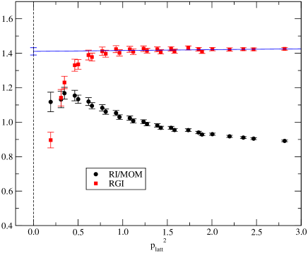
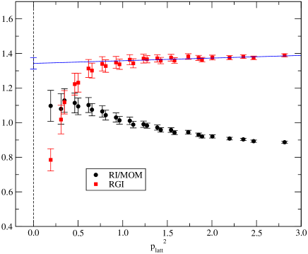
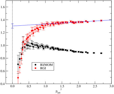
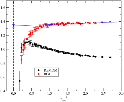
Figure 11: Renormalization factors for the quark mass $Z_{m}$ in RI/MOM scheme (circles) and their RGI values (squares) as functions of $p_{\rm latt}^{2}$ for NF2$\epsilon$ (upper left), NF2p (upper right), NF3p-a (lower left), and NF3p-b (lower right). Results of the linear extrapolation to the $(p_{\rm latt})^{2}\to 0$ limit of $Z_{m}^{\rm RGI}$ are shown as well. For NF2p, NF3p-a and NF3p-b, data with a fixed sea quark mass $m_{\rm sea}(m_{ud})=0.015$ are plotted as an example.

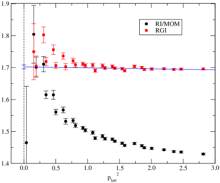
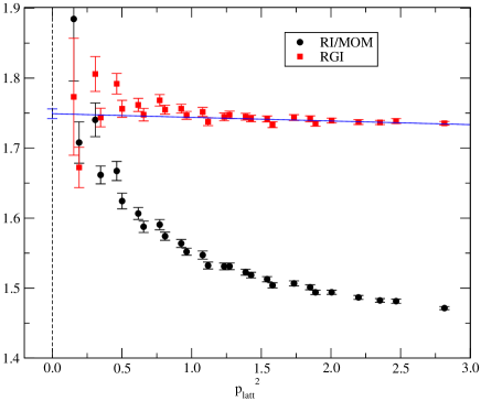
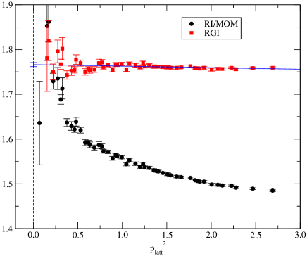
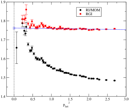
Figure 12: Same as Figure 11 but for the tensor current renormalization factor $Z_{T}$.

The results are plotted in Figures 11 and 12 for $Z_{m}$ and $Z_{T}$, respectively. Filled black symbols representing the numerical data for the RI/MOM scheme clearly show a scale (or $p_{\rm latt}^{2}$) dependence. This dependence can partly be absorbed by perturbatively calculated matching factor $w_{\cal O}^{\rm RI/MOM}(\mu)$ ($\cal O$ = $m$ or $T$) to the RGI values as in the case of $Z_{q}$. The perturbative results for $w_{\cal O}^{\rm RI/MOM}(\mu)$ and $w_{\cal O}^{\overline{\rm MS}}(\mu)$ are summarized in Appendix A.

The numerical data for $Z_{\cal O}^{\rm RGI}=Z_{\cal O}^{\rm RI/MOM}(p_{\rm latt})/w_{\cal O}^{\rm RI/MOM}(p_{\rm latt})$ are also shown in Figures 11 and 12. We find that the scale dependence is largely absorbed at least above $(p_{\rm latt})^{2}\simeq 1$, as expected. Below $(p_{\rm latt})^{2}\simeq 1$ the perturbative estimate of $w_{\cal O}^{\rm RI/MOM}(p)$ becomes less precise even though three- or four-loop calculations are used. Remaining scale dependence above $(p_{\rm latt})^{2}\simeq 1$ is ascribed to the discretization effect of $O(a^{2})$. We therefore extrapolate the data for $Z_{\cal O}^{\rm RGI}$ above $(p_{\rm latt})^{2}=1$ to the vanishing $(p_{\rm latt})^{2}$ limit assuming a linear dependence on $(p_{\rm latt})^{2}$, which is shown by solid lines in Figures 11 and 12.

$m_{\rm sea}(m_{ud})$	$Z_{S}^{\rm RGI}$	$Z_{m}^{\rm RGI}$	$Z_{S}^{\overline{\rm MS}}(2\ {\rm GeV})$	$Z_{m}^{\overline{\rm MS}}(2\ {\rm GeV})$
NF2$\epsilon$, 0.002	0.709(11)	1.411(21)	1.205(18)	0.830(12)
NF2p, 0.015	0.743(18)	1.345(33)	1.263(30)	0.791(19)
0.025	0.719(12)	1.390(24)	1.223(21)	0.818(14)
0.035	0.764(20)	1.308(37)	1.298(35)	0.769(22)
0.050	0.746(16)	1.339(29)	1.268(27)	0.788(17)
0.070	0.726(14)	1.378(26)	1.234(23)	0.810(15)
0.100	0.761(14)	1.313(26)	1.293(24)	0.772(15)
0.000	0.7309(87)	1.366(16)	1.243(15)	0.8035(97)
($\chi^{2}/$dof	1.15	1.15	1.15	1.15)
NF3p-a, 0.015	0.766(19)	1.303(34)	1.296(32)	0.770(20)
0.025	0.734(10)	1.362(20)	1.242(17)	0.805(12)
0.035	0.721(17)	1.386(33)	1.221(29)	0.819(19)
0.050	0.757(15)	1.320(27)	1.281(25)	0.780(16)
0.080	0.765(17)	1.304(31)	1.296(29)	0.770(18)
NF3p-b, 0.015	0.748(11)	1.337(19)	1.265(18)	0.790(11)
0.025	0.7354(62)	1.359(12)	1.245(11)	0.8031(70)
0.035	0.7311(87)	1.368(17)	1.238(15)	0.8078(98)
0.050	0.774(13)	1.289(23)	1.310(22)	0.761(14)
0.100	0.748(13)	1.336(25)	1.266(22)	0.789(15)
“chiral limit”:	0.7325(88)	1.364(16)	1.240(15)	0.8057(97)
($\chi^{2}/$dof	1.61	1.64	1.61	1.64)

Table 8: Renormalization factors of the scalar operator and quark mass in the RGI and in the $\overline{\rm MS}$ schemes at $\mu=2$ GeV. The results at each sea quark mass are listed as well as those in the chiral limit of sea quarks.

$m_{\rm sea}(m_{ud})$	$Z_{T}^{\rm RGI}$	$Z_{T}^{\overline{\rm MS}}(2\ {\rm GeV})$
NF2$\epsilon$, 0.002	1.7023(62)	1.4689(53)
NF2p, 0.015	1.7461(69)	1.5066(59)
0.025	1.7418(63)	1.5030(54)
0.035	1.7393(70)	1.5008(61)
0.050	1.7470(72)	1.5075(62)
0.070	1.7361(63)	1.4981(54)
0.100	1.7330(64)	1.4953(55)
0.000	1.7441(38)	1.5050(33)
($\chi^{2}/$dof	0.24	0.24)
NF3p-a, 0.015	1.7662(44)	1.5283(38)
0.025	1.7663(50)	1.5284(43)
0.035	1.7685(54)	1.5303(47)
0.050	1.7591(38)	1.5222(33)
0.080	1.7674(48)	1.5294(41)
NF3p-b, 0.015	1.7620(43)	1.5247(37)
0.025	1.7630(42)	1.5255(37)
0.035	1.7637(42)	1.5261(36)
0.050	1.7518(43)	1.5159(37)
0.100	1.7640(56)	1.5264(48)
“chiral limit”:	1.7639(35)	1.5262(30)
($\chi^{2}/$dof	1.18	1.18)

Table 9: Same as Table 8 but for $Z_{T}$.

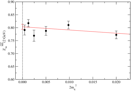
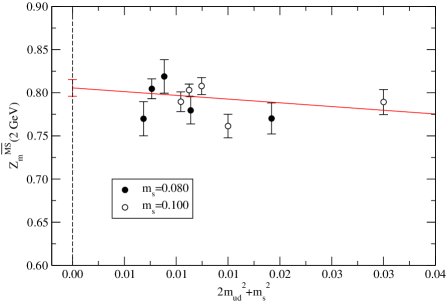
Figure 13: Left panel: $Z_{m}^{\overline{\rm MS}}(2\ {\rm GeV})$ for NF2p as a function of $2m_{\rm sea}^{2}$. Right panel: Same value for NF3p-a and NF3p-b as a function of $2m_{ud}^{2}+m_{s}^{2}$. Linear extrapolation to the $m_{\rm sea}=0$ limit or the $m_{ud}=0$ limit is shown as well.

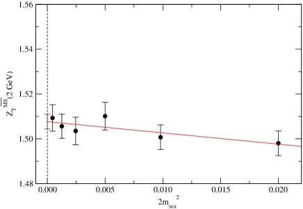
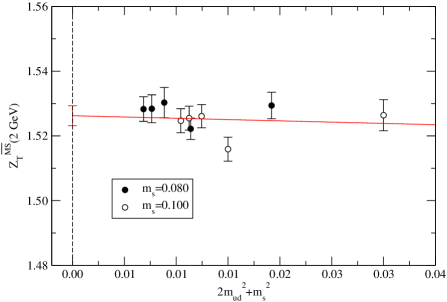
Figure 14: Same as Figure 13 but for $Z_{T}^{\overline{\rm MS}}(2\ {\rm GeV})$.

The renormalization constants in the $\overline{\rm MS}$ scheme are obtained as $Z_{\cal O}^{\overline{\rm MS}}(\mu)=w_{\cal O}^{\overline{\rm MS}}(\mu)\cdot Z_{\cal O}^{\rm RGI}$, again using the matching factor to the RGI value $w_{\cal O}^{\overline{\rm MS}}(\mu)$. Results of the RGI value and those in the $\overline{\rm MS}$ scheme at $\mu$ = 2 GeV are listed in Table 8 for ${\cal O}$ = $m$ and $S$ with the four-loop level matching, and in Table 9 for ${\cal O}=T$ with the three-loop level.

For the NF2p ensembles the renormalization factors at finite sea quark masses are extrapolated to the limit of $m_{\rm sea}=0$ as a linear function of $2m_{\rm sea}^{2}$. For the 2+1-flavor data, we combine NF3p-a and NF3p-b to quote the final result in the chiral limit of all of the three flavors, assuming a sea quark mass dependence of the form $Z(1+c^{(3)}(2m_{ud}^{2}+m_{s}^{2}))$. The extrapolation is shown in Figures 13 and 14 for the NF2p (left panel) and NF3p-a/b (right panel) ensembles. Although we do not observe any systematic sea quark mass dependence, the data show larger fluctuations than the statistical errors at each sea quark mass for $Z_{m}$. As a result, the $\chi^{2}/$dof for the combination of NF3p-a and NF3p-b is uncomfortably large ($\sim$ 2.6), as listed in Tables  8. This may indicate that the statistical error estimated at each sea quark mass is underestimated. It is also suggested from the size of the statistical error at a fixed sea quark mass, say $m_{\rm sea}$ (or $m_{ud}$) = 0.015. Namely, the size of error is comparable between NF2p and NF3p-a/b, though the statistics is more than factor of two larger for NF2p. We use the jackknife method for the statistical analysis with a bin size of 50 HMC trajectories. Given the limited total length of trajectories (2,500 for NF3p-a/b), the statistical error does not change much even if we increase the bin size to 100 trajectories. We do not investigate this point further, because the statistical error does not give the dominant part of the error in the final results.

For the central values of the final results, we quote the result at $m_{\rm sea}=0.002$ for NF2$\epsilon$ and that in the $m_{\rm sea}=0$ limit for NF2p or in the $m_{ud}=m_{s}=0$ limit for the combination of NF3p-a and NF3p-b. In Table 8, the extrapolated values are listed in separated rows. The results for $Z_{m}$ are

$$Z_{m}^{\overline{\rm MS}}(2\ {\rm GeV})=\left\{\begin{array}[]{l}0.824(14)(24)\left({}^{+14}_{-00}\right)\ \ {\rm for\ }N_{f}=2,\ \beta=2.35\\ 0.804(10)(25)\left({}^{+00}_{-21}\right)\ \ {\rm for\ }N_{f}=2,\ \beta=2.30\\ 0.806(12)(24)\left({}^{+00}_{-11}\right)\ \ {\rm for\ }N_{f}=2+1,\beta=2.30,\\ \end{array}\right.$$ (III.26)

The first error is statistical, which includes the small statistical errors in the extraction of $Z_{A}^{\rm WTI}$ and the lattice scale $a^{-1}$. The scale affects the determination of the matching point $\mu=2$ GeV. On this error, we also take account of the ambiguity in removing the scale dependence of $Z_{m}^{\rm RGI}$ by comparing the results with different ranges of the linear fit. The systematic errors given in the second and third parentheses are described in the following.

An important source of the systematic error is the truncation of the perturbative expansion in the matching between the RI/MOM and $\overline{\rm MS}$ schemes. It is given by a ratio of two matching factors to the Renormalization Group Invariant (RGI) value, i.e. $w_{m}^{\rm RI/MOM}(\mu)$ and $w_{m}^{\overline{\rm MS}}(\mu)$ in (A.27). The perturbative expansion of these factors is given in (A.28) and known to four-loop order. By setting $\mu$ = 2 GeV, we may evaluate how it depends on the loop order. For $N_{f}=2$, the ratio $w_{m}^{\overline{\rm MS}}(\mu)/w_{m}^{\rm RI/MOM}(\mu)$ becomes 1, 0.911, 0.863, and 0.835 when the perturbative expansion includes $O(\alpha_{s}^{0})$, $O(\alpha_{s}^{1})$, $O(\alpha_{s}^{2})$, and $O(\alpha_{s}^{3})$ terms respectively. From this observation, we find that the perturbative expansion converges such that the additional correction is about 60% of the correction of the previous order. Same level of the correction is observed for the case of $N_{f}=2+1$. We therefore assume that this convergence persists at the next unknown perturbative coefficient. The second error in (III.26) is estimated by taking a difference of the current best four-loop analysis and the second best three-loop analysis and multiplying a factor 0.6.

The effect of SCSB may arise in two different ways. First, in the extraction of $Z_{q}$ we used the axial-vector vertex function $\Lambda_{A}$, but if we used the vector vertex function $\Lambda_{V}$ instead the result is slightly shifted, which is given in the third parentheses. Note that this does not matter for NF2$\epsilon$, because there is no significant difference between $\Lambda_{V}$ and $\Lambda_{A}$ in the $\epsilon$-regime. Second, one may expect some uncertainty in the process of subtraction of the power divergent piece from $\langle\bar{q}q\rangle^{(N)}$. In Section III.3, we demonstrate that the power-divergent term can be removed from $\left\langle\bar{q}q\right\rangle^{(N)}$ to obtain $\left\langle\bar{q}q\right\rangle^{\rm(subt)}$ in almost $N$-independent way. However, it does not guarantee that the results for $\left\langle\bar{q}q\right\rangle^{\rm(subt)}$ are unchanged beyond the maximum value of $N$ we studied. In fact, in the $p$-regime, we find that $\Sigma\equiv\left\langle\bar{q}q\right\rangle^{(\rm subt)}(m_{q}=0)$ obtained with various values of $N$ slightly increases as a function of $N$. In the calculation based on the chiral perturbation theory on the same ensembles Fukaya et al. (2007a, 2009), we find $\approx 10\%$ larger values of $\Sigma$ than those from the eigenvalue decomposition for NF2p and NF3p-a/b. For NF2$\epsilon$, the result of the calculation based on the chiral random matrix theory Fukaya et al. (2007b) is $\approx 10\%$ smaller. To estimate the effect of the truncation of eigenvalues, we repeat the same analysis by fixing the value of $\Sigma$ 10% smaller (larger) than the original one for NF2$\epsilon$ (NF2p and NF3p-a/b). As a result, we find the magnitude of finite $N$ effect is similar to the statistical errors for all cases. We quote the difference from the central value in the third error in (III.26). For NF2p and NF3p-a/b, we combine this error with the effect from the difference between $\Lambda_{A}$ and $\Lambda_{V}$, which is in the same direction.

For completeness, we also present results for $Z_{T}$. Matching procedures are illustrated in Figure 12. Table 9 summarizes the RGI and the $\overline{\rm MS}$ values. The left and right panels in Figure 14 show the linear extrapolation as a function of $2m_{\rm sea}^{2}$ (NF2p) and $2m_{ud}^{2}+m_{s}^{2}$ (NF3p-a/b), respectively.

IV Conclusion

We calculated the renormalization factors for the quark bilinear operators constructed from the overlap fermion formulation, based on the original idea of NPR proposed in Martinelli et al. (1995). The aim of this calculation is to provide the renormalization factors for a series of numerical studies being performed by the JLQCD and TWQCD collaborations using dynamical overlap fermions. By virtue of the exact chiral symmetry of the overlap fermion, the analysis is largely simplified compared to other non-chiral fermion formulations.

Through the simulation in the $\epsilon$-regime, we explicitly confirm that the vector and axial-vector vertex functions agree with each other when the effect of spontaneous chiral symmetry breaking is negligible. This may provide a clean way to calculate the renormalization factors through the NPR method, since the calculation does not suffer from the potential problems due to pion poles.

In the $p$-regime, where the spontaneous symmetry breaking effectively remains even on a finite volume lattice, we may precisely control the non-perturbative quark mass dependence of the quark propagator and vertex functions using the OPE analysis supplemented by the condensate explicitly constructed from the low-lying quark eigenmodes. The exact chiral symmetry of the overlap fermion plays an important role also in this analysis.

Our main results are those of the mass renormalization factor $Z_{m}$, which is an inverse of the scalar density renormalization factor $Z_{S}$. The result has been already used in the calculation of the chiral condensate in two-flavor QCD from the Dirac operator spectrum Fukaya et al. (2007b, 2008) and from the topological susceptibility Chiu et al. (2009). It has also been used in our calculation of up and down quark mass through the analysis of pion mass and decay constant Noaki et al. (2008a). Extension of these works to the 2+1-flavor case is in progress.

By using the value of $Z_{m}^{\overline{\rm MS}}$ we quoted in this article, we are planning to determine the up and down quark mass $m_{ud}$ and the strange quark mass $m_{s}$ from the analysis of the meson masses $m_{\pi}^{2}$ and $m_{K}^{2}$ and the decay constants $f_{\pi}$ and $f_{K}$ in the $N_{f}=2+1$ dynamical simulation. A preliminary results from this project was reported in Noaki et al. (2008b).

Appendix A Perturbative matching

In this appendix, we present the details of our matching procedure.

The matching of an operator ${\cal O}$ between the $\overline{\rm MS}$ scheme and the RI/MOM scheme is written as

$${\cal O}^{\overline{\rm MS}}(\mu)=\frac{w_{\cal O}^{\overline{\rm MS}}(\mu)}{w_{\cal O}^{\rm RI/MOM}(\mu_{0})}{\cal O}^{\rm RI/MOM}(\mu_{0}),$$ (A.27)

where the conversion factor $w_{\cal O}^{X}(\mu)$ from a given scheme $X$ to the so-called Renormalization Group Invariant (RGI) value is written as

$$w_{\cal O}^{X}(\mu) = \alpha_{S}(\mu)^{\bar{\gamma}_{0}}\Biggl{[}1+(\bar{\gamma}_{1}-\bar{\beta}_{1}\bar{\gamma}_{0})\frac{\alpha_{S}(\mu)}{4\pi}$$ (A.28)

$$+\tfrac{1}{2}\left((\bar{\gamma}_{1}-\bar{\beta}_{1}\bar{\gamma}_{0})^{2}+\bar{\gamma}_{2}+\bar{\beta}_{1}^{2}\bar{\gamma}_{0}-\bar{\beta}_{1}\bar{\gamma}_{1}-\bar{\beta}_{2}\bar{\gamma}_{0}\right)\left(\frac{\alpha_{S}(\mu)}{4\pi}\right)^{2}$$

$$+\Bigl{(}\tfrac{1}{6}(\bar{\gamma}_{1}-\bar{\beta}_{1}\bar{\gamma}_{0})^{3}+\tfrac{1}{2}(\bar{\gamma}_{1}-\bar{\beta}_{1}\bar{\gamma}_{0})(\bar{\gamma}_{2}+\bar{\beta}_{1}^{2}\bar{\gamma}_{0}-\bar{\beta}_{1}\bar{\gamma}_{1}-\bar{\beta}_{2}\bar{\gamma}_{0})$$

$$+\tfrac{1}{3}(\bar{\gamma}_{3}-\bar{\beta}_{1}^{3}\bar{\gamma}_{0}+2\bar{\beta}_{1}\bar{\beta}_{2}\bar{\gamma}_{0}-\bar{\beta}_{3}\bar{\gamma}_{0}+\bar{\beta}_{1}^{2}\bar{\gamma}_{1}-\bar{\beta}_{2}\bar{\gamma}_{1}-\bar{\beta}_{1}\bar{\gamma}_{2})\Bigr{)}\left(\frac{\alpha_{S}(\mu)}{4\pi}\right)^{3}\Biggr{]}_{X},$$

to the four-loop order in terms of the strong coupling constant $\alpha_{S}(\mu)$. (For the coupling constant, we always use the $\overline{\rm MS}$ scheme.) The coefficients $\bar{\beta}_{i}$ and $\bar{\gamma}_{i}$ are given in terms of the coefficients of the $\beta$-function $\beta(\alpha_{S})$ and the anomalous dimension $\gamma_{\cal O}(\alpha_{S})$

$$\beta = -\beta_{0}\frac{\alpha_{S}^{2}}{4\pi}-\beta_{1}\frac{\alpha_{S}^{3}}{(4\pi)^{2}}-\beta_{2}\frac{\alpha_{S}^{4}}{(4\pi)^{3}}-\beta_{3}\frac{\alpha_{S}^{5}}{(4\pi)^{4}}-\cdots,$$ (A.29)

$$\gamma_{\cal O} = -\gamma_{\cal O}^{(0)}\frac{\alpha_{S}}{4\pi}-\gamma_{\cal O}^{(1)}\left(\frac{\alpha_{S}}{4\pi}\right)^{2}-\gamma_{\cal O}^{(2)}\left(\frac{\alpha_{S}}{4\pi}\right)^{3}-\gamma_{\cal O}^{(3)}\left(\frac{\alpha_{S}}{4\pi}\right)^{4}-\cdots.$$ (A.30)

as $\bar{\beta}_{i}=\beta_{i}/\beta_{0}$ and $\bar{\gamma}_{i}=\gamma_{\cal O}^{(i)}/\beta_{0}$.

The $\beta$-function is specified by

$$\beta_{0} = 11-\frac{2}{3}N_{f},$$ (A.31)

$$\beta_{1} = 102-\frac{38}{3}N_{f},$$ (A.32)

$$\beta_{2} = \frac{2857}{2}-\frac{5033}{18}N_{f}+\frac{325}{54}N_{f}^{2},$$ (A.33)

$$\beta_{3} = \frac{149753}{6}+3564\zeta_{3}-\left(\frac{1078361}{162}+\frac{6508}{27}\zeta_{3}\right)N_{f}$$ (A.34)

$$+\left(\frac{50065}{162}+\frac{6472}{81}\zeta_{3}\right)N_{f}^{2}+\frac{1093}{729}N_{f}^{3},$$

with $\zeta_{3}$ = 1.2020569. The running coupling constant is then obtained as

$$\alpha_{S}(\mu) = \frac{4\pi}{\beta_{0}\ln\mu^{2}/\Lambda^{2}}\Biggl{[}1-\frac{\beta_{1}}{\beta_{0}^{2}}\frac{\ln\left(\ln\mu^{2}/\Lambda^{2}\right)}{\ln\mu^{2}/\Lambda^{2}}$$ (A.35)

$$+\frac{\beta_{1}^{2}}{\beta_{0}^{4}\left(\ln\mu^{2}/\Lambda^{2}\right)^{2}}\left(\left(\ln\ln\mu^{2}/\Lambda^{2}\right)^{2}-\ln\left(\ln\mu^{2}/\Lambda^{2}\right)+\frac{\beta_{2}\beta_{0}}{\beta_{1}^{2}}-1\right)$$

$$-\frac{\beta_{1}^{3}}{\beta_{0}^{6}\left(\ln\mu^{2}/\Lambda^{2}\right)^{3}}\Biggl{(}\left(\ln\ln\mu^{2}/\Lambda^{2}\right)^{3}-\frac{5}{2}\left(\ln\ln\mu^{2}/\Lambda^{2}\right)^{2}$$

$$\hskip 110.96556pt-\left(2-\frac{3\beta_{0}\beta_{2}}{\beta_{1}^{2}}\right)\ln\ln\mu^{2}/\Lambda^{2}+\frac{1}{2}-\frac{\beta_{0}^{2}\beta_{3}}{2\beta_{1}^{3}}\Biggr{)}\Biggr{]}.$$

In our work, we chose $\Lambda$ = 245 MeV for both 2 and 2+1-flavor analysis.

The renormalization of the scalar bilinear operator ${\cal O}=S=\bar{q}q$ is an inverse of the mass renormalization. The anomalous dimension thus has a relation $\gamma_{m}=-\gamma_{\rm S}$. At the lowest order, $\gamma_{m}^{(0)}=4$ for any scheme. Higher order coefficients are calculated in Chetyrkin and Retey (2000) to the four-loop order in the RI/MOM scheme

$$\gamma_{m}^{(1)} = 126-\frac{52}{9}N_{f},$$ (A.36)

$$\gamma_{m}^{(2)} = \frac{20911}{3}-\frac{3344}{3}\zeta_{3}+\left(-\frac{18386}{27}+\frac{128}{9}\zeta_{3}\right)N_{f}+\frac{928}{81}N_{f}^{2},$$ (A.37)

$$\gamma_{m}^{(3)} = \frac{300665987}{648}-\frac{15000871}{108}\zeta_{3}+\frac{6160}{3}\zeta_{5}+\left(-\frac{7535473}{108}+\frac{627127}{54}\zeta_{3}+\frac{4160}{3}\zeta_{5}\right)N_{f}$$ (A.38)

$$+\left(\frac{670948}{243}-\frac{6416}{27}\zeta_{3}\right)N_{f}^{2}-\frac{18832}{729}N_{f}^{3},$$

and in the $\overline{\rm MS}$ scheme

$$\gamma_{m}^{(1)} = \frac{202}{3}-\frac{20}{9}N_{f},$$ (A.39)

$$\gamma_{m}^{(2)} = 1249-\left(\frac{2216}{27}+\frac{160}{3}\zeta_{3}\right)N_{f}-\frac{140}{81}N_{f}^{2},$$ (A.40)

$$\gamma_{m}^{(3)} = \frac{4603055}{162}+\frac{135680}{27}\zeta_{3}-8800\zeta_{5}-\left(\frac{91723}{27}+\frac{34192}{9}\zeta_{3}-880\zeta_{4}-\frac{18400}{9}\zeta_{5}\right)N_{f}$$ (A.41)

$$+\left(\frac{5242}{243}+\frac{800}{9}\zeta_{3}-\frac{160}{3}\zeta_{4}\right)N_{f}^{2}-\left(\frac{332}{243}-\frac{64}{27}\zeta_{3}\right)N_{f}^{3},$$

where $\zeta_{3}=1.202057$, $\zeta_{4}=\pi^{4}/90$ and $\zeta_{5}=1.036928$.

For the quark field renormalization (${\cal O}=q$), the lowest order coefficient vanishes in the Landau gauge for any scheme. The higher order coefficients for the RI/MOM scheme are Chetyrkin and Retey (2000)

$$\gamma_{q}^{(1)} = \frac{67}{3}-\frac{4}{3}N_{f},$$ (A.42)

$$\gamma_{q}^{(2)} = \frac{43477}{36}-\frac{607}{2}\zeta_{3}-\left(\frac{3674}{27}-16\zeta_{3}\right)N_{f}+\frac{80}{27}N_{f}^{2},$$ (A.43)

$$\gamma_{q}^{(3)} = \frac{54714743}{648}-\frac{7004309}{162}\zeta_{3}+\frac{15846715}{1296}\zeta_{5}-\left(\frac{4659455}{324}-\frac{637413}{162}\zeta_{3}+830\zeta_{5}\right)N_{f}$$ (A.44)

$$+\left(\frac{166269}{243}-64\zeta_{3}\right)N_{f}^{2}-\frac{688}{81}N_{f}^{3},$$

while the $\overline{\rm MS}$ coefficients are

$$\gamma_{q}^{(1)} = \frac{67}{3}-\frac{4}{3}N_{f},$$ (A.45)

$$\gamma_{q}^{(2)} = \frac{20729}{36}-\frac{79}{2}\zeta_{3}-\frac{550}{9}N_{f}+\frac{20}{27}N_{f}^{2},$$ (A.46)

$$\gamma_{q}^{(3)} = \frac{2109389}{162}-\frac{565939}{324}\zeta_{3}+\frac{2607}{4}\zeta_{4}-\frac{761525}{1296}\zeta_{5}-\left(\frac{162103}{81}+\frac{2291}{27}\zeta_{3}+\frac{79}{2}\zeta_{4}+\frac{160}{3}\zeta_{5}\right)N_{f}$$ (A.47)

$$+\left(\frac{3853}{81}+\frac{160}{9}\zeta_{3}\right)N_{f}^{2}+\frac{140}{243}N_{f}^{3}.$$

Coefficients for the tensor current ${\cal O}=T=\bar{q}\sigma_{\mu\nu}q$ are known to three-loop Gracey (2003); Aoki et al. (2008a). Besides the common value $\gamma_{T}^{(0)}=4/3$, higher order coefficients for the RI/MOM scheme are

$$\gamma_{T}^{(1)} = \frac{362}{9}-\frac{52}{27}N_{f},$$ (A.48)

$$\gamma_{T}^{(2)} = \frac{159607}{81}-\frac{13072}{27}\zeta_{3}+\left(-\frac{17426}{81}+\frac{256}{27}\zeta_{3}\right)N_{f}+\frac{928}{243}N_{f}^{2},$$ (A.49)

and those for the $\overline{\rm MS}$ scheme are

$$\gamma_{T}^{(1)} = \frac{362}{9}-\frac{52}{27}N_{f},$$ (A.50)

$$\gamma_{T}^{(2)} = \frac{52555}{81}-\frac{928}{27}\zeta_{3}-\left(\frac{5240}{81}+\frac{160}{9}\zeta_{3}\right)N_{f}-\frac{4}{9}N_{f}^{2}.$$ (A.51)

References

- Martinelli et al. (1995) G. Martinelli, C. Pittori, C. T. Sachrajda, M. Testa, and A. Vladikas, Nucl. Phys. B445, 81 (1995), eprint hep-lat/9411010.
- Blum et al. (2002) T. Blum et al., Phys. Rev. D66, 014504 (2002), eprint hep-lat/0102005.
- Aoki et al. (2008a) Y. Aoki et al., Phys. Rev. D78, 054510 (2008a), eprint arXiv:0712.1061 [hep-lat].
- DeGrand and Liu (2005) T. A. DeGrand and Z.-f. Liu, Phys. Rev. D72, 054508 (2005), eprint hep-lat/0507017.
- Zhang et al. (2005) J. B. Zhang et al., Phys. Rev. D72, 114509 (2005), eprint hep-lat/0507022.
- Galletly et al. (2007) D. Galletly et al., Phys. Rev. D75, 073015 (2007), eprint hep-lat/0607024.
- Aoki et al. (2008b) S. Aoki et al. (JLQCD), Phys. Rev. D78, 014508 (2008b), eprint arXiv:0803.3197 [hep-lat].
- Hashimoto et al. (2007) S. Hashimoto et al. (JLQCD), PoS LAT2007, 101 (2007), eprint arXiv:0710.2730 [hep-lat].
- Matsufuru et al. (2008) H. Matsufuru et al. (JLQCD and TWQCD), PoS LAT2008, 077 (2008).
- Fukaya et al. (2007a) H. Fukaya et al., Phys. Rev. D76, 054503 (2007a), eprint arXiv:0705.3322 [hep-lat].
- Fukaya et al. (2007b) H. Fukaya et al. (JLQCD), Phys. Rev. Lett. 98, 172001 (2007b), eprint hep-lat/0702003.
- Fukaya et al. (2008) H. Fukaya et al. (JLQCD), Phys. Rev. D77, 074503 (2008), eprint arXiv:0711.4965 [hep-lat].
- Aoki et al. (2008c) S. Aoki et al. (JLQCD and TWQCD), Phys. Lett. B665, 294 (2008c), eprint arXiv:0710.1130 [hep-lat].
- Chiu et al. (2009) T.-W. Chiu, T.-H. Hsieh, and P.-K. Tseng (TWQCD), Phys. Lett. B671, 135 (2009), eprint arXiv:0810.3406 [hep-lat].
- Noaki et al. (2008a) J. Noaki et al. (JLQCD and TWQCD), Phys. Rev. Lett. 101, 202004 (2008a), eprint arXiv:0806.0894 [hep-lat].
- Noaki et al. (2008b) J. Noaki et al., PoS LAT2008, 107 (2008b), eprint arXiv:0810.1360 [hep-lat].
- Neuberger (1998a) H. Neuberger, Phys. Lett. B417, 141 (1998a), eprint hep-lat/9707022.
- Neuberger (1998b) H. Neuberger, Phys. Lett. B427, 353 (1998b), eprint hep-lat/9801031.
- Duane et al. (1987) S. Duane, A. D. Kennedy, B. J. Pendleton, and D. Roweth, Phys. Lett. B195, 216 (1987).
- Fukaya et al. (2006) H. Fukaya et al. (JLQCD), Phys. Rev. D74, 094505 (2006), eprint hep-lat/0607020.
- Aoki et al. (2007) S. Aoki, H. Fukaya, S. Hashimoto, and T. Onogi, Phys. Rev. D76, 054508 (2007), eprint arXiv:0707.0396 [hep-lat].
- Shintani et al. (2009) E. Shintani et al. (JLQCD), Phys. Rev. D79, 074510 (2009), eprint arXiv:0807.0556 [hep-lat].
- Sturm et al. (2009) C. Sturm et al. (2009), eprint arXiv: 0901.2599 [hep-ph].
- Giusti and Vladikas (2000) L. Giusti and A. Vladikas, Phys. Lett. B488, 303 (2000), eprint hep-lat/0005026.
- Politzer (1976) H. D. Politzer, Nucl. Phys. B117, 397 (1976).
- Gasser and Leutwyler (1984) J. Gasser and H. Leutwyler, Ann. Phys. 158, 142 (1984).
- Damgaard and Fukaya (2009) P. H. Damgaard and H. Fukaya, JHEP 01, 052 (2009), eprint arXiv:0812.2797 [hep-lat].
- Aoki et al. (2009) S. Aoki et al. (JLQCD and TWQCD) (2009), eprint arXiv:0905.2465 [hep-lat].
- Fukaya et al. (2009) H. Fukaya et al. (JLQCD) (2009), eprint in preparation.
- Chetyrkin and Retey (2000) K. G. Chetyrkin and A. Retey, Nucl. Phys. B583, 3 (2000), eprint hep-ph/9910332.
- Gracey (2003) J. A. Gracey, Nucl. Phys. B662, 247 (2003), eprint hep-ph/0304113.