Three Dimensional Modeling of Hot Jupiter Atmospheric Flows

Abstract

We present a three dimensional hot Jupiter model, extending from 200 bar to 1 mbar, using the Intermediate General Circulation Model from the University of Reading. Our horizontal spectral resolution is T31 (equivalent to a grid of 48$\times$96), with 33 logarithmically spaced vertical levels. A simplified (Newtonian) scheme is employed for the radiative forcing. We adopt a physical set up nearly identical to the model of HD 209458b by Cooper & Showman (2005, 2006) to facilitate a direct model inter-comparison. Our results are broadly consistent with theirs but significant differences also emerge. The atmospheric flow is characterized by a super-rotating equatorial jet, transonic wind speeds, and eastward advection of heat away from the dayside. We identify a dynamically-induced temperature inversion (“stratosphere”) on the planetary dayside and find that temperatures at the planetary limb differ systematically from local radiative equilibrium values, a potential source of bias for transit spectroscopic interpretations. While our model atmosphere is quasi-identical to that of Cooper & Showman (2005, 2006) and we solve the same meteorological equations, we use different algorithmic methods, spectral-implicit vs. grid-explicit, which are known to yield fully consistent results in the Earth modeling context. The model discrepancies identified here indicate that one or both numerical methods do not faithfully capture all of the atmospheric dynamics at work in the hot Jupiter context. We highlight the emergence of a shock-like feature in our model, much like that reported recently by Showman et al. (2009), and suggest that improved representations of energy conservation may be needed in hot Jupiter atmospheric models, as emphasized by Goodman (2009).

1 Introduction

Hot Jupiter atmospheres challenge our understanding of meteorology, introducing a new regime in which the atmospheric conditions are significantly different from the more familiar solar system cases. Common assumptions used in classic atmospheric dynamics may break down and hot Jupiter models may require the inclusion of new physics. These planets orbit their parent stars with periods of a few days and are expected to be tidally locked, with permanent daysides subject to intense stellar irradiation. This strong, asymmetric heating is clearly unique, but hot Jupiters also differ from their namesake Jupiter in that their rotation periods are much longer (several days instead of 10 hours), so that the size of dynamical atmospheric structures should be much larger in scale (Showman & Guillot, 2002; Menou et al., 2003). For a detailed discussion of the characteristics of this new regime see the recent review by Showman et al. (2008b). This novel type of planetary atmosphere challenges us to develop models that can correctly treat the physics at work and thus be used to interpret recent ground-breaking observations.

Aside from the inherently interesting properties of hot Jupiters, they have also garnered attention because of impressive direct detections of their atmospheres, which give theorists the opportunity to test their models against reality. The first observations of thermal emission from the daysides of hot Jupiters (Charbonneau et al., 2005; Deming et al., 2005), have been followed by multiwavelength measurements (Charbonneau et al., 2008; Knutson et al., 2008, 2009b), the detection of a surprisingly bright planet (Harrington et al., 2007), observations of a Neptune-mass planet (Deming et al., 2007; Demory et al., 2007), and multi-epoch observations (Agol et al., 2009). Orbital phase curves, which measure the variation in emission as different longitudes on the planet rotate into view, have been obtained (Harrington et al., 2006; Cowan et al., 2007; Knutson et al., 2007, 2009a). This same observational technique has been used to witness the effect of flash-heating on a highly eccentric planet (Laughlin et al., 2009). We are also able to determine the composition and something of the vertical temperature profile of these planets from transmission spectra (Charbonneau et al., 2002; Tinetti et al., 2007; Pont et al., 2008; Sing et al., 2008; Swain et al., 2008b) as starlight filters through the planet’s atmosphere, and the planet’s own emission spectrum (Grillmair et al., 2007; Richardson et al., 2007; Swain et al., 2008a). In light of these increasingly detailed constraints, we must continue to improve our atmospheric models, to reach a better understanding of the basic physics at work and grow confidence in that we have correctly captured the relevant processes.

Decades of work have gone into developing complex codes to model the dynamics of the Earth’s atmosphere, with extensions to include other planetary bodies in our Solar System. For the Earth, we have the benefit of being able to directly compare the model results to the circulation patterns observed in situ. So far for hot Jupiters we only have basic, disk-integrated, usually single-epoch observations, making it more difficult to test the reliability of model results. There exists a wide range of hot Jupiter models in the literature, which employ a variety of methods and assumptions to approach this novel regime (Cho et al., 2003, 2008; Burkert et al., 2005; Cooper & Showman, 2005, 2006; Langton & Laughlin, 2007; Dobbs-Dixon & Lin, 2008; Showman et al., 2008a, 2009). Comparing the various models used against each other is important to test their numerical and physical consistency.

Comparisons between atmospheric codes is standard practice in Earth modeling. Held & Suarez (1994) presented a benchmark comparison between two dynamical cores, i.e. codes solving the dynamical equations independently of radiative forcing, for a simplified Earth model. Given an identical, idealized physical set-up, they found excellent quantitative agreement between the two numerical codes, suggesting that each code was accurately solving the meteorological equations in the Earth regime. We would like to gain this level of confidence in hot Jupiter circulation models. Here we use a pseudo-spectral, semi-implicit code to solve the same set of equations and atmospheric conditions as done by Cooper & Showman (2005, 2006, hereafter C&S) with the grid-based, time explicit ARIES/GEOS dynamical core (Suarez & Takacs, 1995). The ARIES/GEOS code is identical to, and the IGCM conceptually similar to, the codes compared by Held & Suarez (1994), although they are applied here to an entirely new circulation regime. We pay special attention to various details in our model results in order to facilitate potential comparisons with other codes in the future. Disparities in model results for an identical physical setup should help us understand how the different algorithms deviate in the regime of relevance to hot Jupiters and presumably lead us to the identification of any additional physics that may be needed for the accurate modeling of hot Jupiter atmospheres.

In §2 we introduce the code used and detail our physical and numerical set up. We present our results by first showing horizontal structures at different vertical levels in §3.1 and then presenting vertical structure in §3.2. We compare our results with those of C&S in §4.1, discuss issues of vertical exchange between the upper and lower regions of the atmosphere in §4.2, and in §4.3 provide a detailed discussion of the shock-like feature found in our simulated flow. We summarize our most significant findings and conclude in §5.

2 The Model

We use the Intermediate General Circulation Model (IGCM) developed at the University of Reading (Hoskins & Simmons, 1975). This is a well-tested and accurate solver of the primitive equations of meteorology: the three dimensional fluid equations applied to a shallow ideal gas atmosphere in hydrostatic balance on a rotating sphere. We use the first version of the code (IGCM1) in which radiative forcing is implemented through a Newtonian relaxation scheme. This pseudo-spectral, semi-implicit code is described in more detail in Menou & Rauscher (2009), but we repeat salient points here.

The vertical coordinate used is $\sigma=p/p_{s}$, where $p_{s}$ is the pressure at the bottom boundary and can vary horizontally. In the run presented here we obtain surface pressure variations of at most 0.5%. Thus each $\sigma$ level is fairly well represented by a constant pressure, and for clarity of presentation we will refer to each level by its average pressure. Our figures will likewise use pressure as the vertical coordinate.

The model solves the flow in a frame that is rotating with the bulk planetary interior, which is assumed to be precisely synchronized with the orbit. In the remainder of this paper, we refer to planet days as equal to the rotational (and orbital) period of the planet.

The radiative forcing is treated through the method of Newtonian relaxation. The diabatic heating and cooling rate at every point in the atmosphere is given by

$$Q_{T}=\frac{T_{\mathrm{eq}}(\sigma,\lambda,\phi)-T}{\tau_{\mathrm{rad}}(\sigma)}$$ (1)

where the local temperature, $T$, relaxes to the prescribed equilibrium profile, $T_{\mathrm{eq}}$, on the radiative timescale defined by $\tau_{\mathrm{rad}}$. We describe our particular choice of $T_{\mathrm{eq}}$ in the next section.

To model the effects of dissipation on small scales, hyperdissipation acts upon the vertical component of the flow relative vorticity, the flow divergence, and the temperature fields as:

$$Q_{\mathrm{vor,div,}T}=-\nu_{\mathrm{diss}}\nabla^{8}[\mathrm{vor,div,}T]$$ (2)

where the coefficient $\nu_{\mathrm{diss}}$ ($=8.54\times 10^{47}$ m⁸ s^-1 in the present model) is chosen so that the smallest resolved structures are diffused in a small fraction of a planet day.

There are several key distinctions between the work done here and in Menou & Rauscher (2009). We have significantly extended our vertical domain, using logarithmically spaced levels to model an atmosphere from 1 mbar to 220 bar. In this paper the radiative timescale is not constant, but increases with depth in the atmosphere. We have also chosen a relaxation temperature profile (described in detail below) with the strongest day-night temperature differences at the top of the atmosphere. The significant variations with height introduced in this deep model apparently prevent the same barotropic (vertically aligned) behavior as reported in Menou & Rauscher (2009).

2.1 Parameter choices

We have chosen physical and model parameters so as to match the model in C&S as closely as possible, which is set up for the hot Jupiter HD 209458b. Specifically, we adopt the same values for the planetary radius, gravitational acceleration, and rotation rate: $R_{p}=$ 9.44$\times 10^{7}$ m, $g=$ 9.42 m s^-2, and $\Omega_{p}=$ 2.06$\times 10^{-5}$ rad s^-1. We use the same specific gas constant, $\mathcal{R}=4593$ J kg^-1 K^-1, and $\kappa=\mathcal{R}/c_{p}=0.321$. The horizontal resolution in C&S is approximately [5^o, 4^o] in longitude and latitude. We run at T31 resolution, which corresponds to a resolution slightly under 4^o in both dimensions. The model in C&S spans a range from 1 mbar to 3 kbar with 40 logarithmically spaced vertical levels. We use the same vertical resolution, but only model down to 220 bar (using 33 levels) so that our bottom boundary is safely above the transition to the interior adiabat at $\sim$1 kbar (Iro et al., 2005) since this version of our IGCM code does not include any special treatment for convective columns.

As in C&S we use the work by Iro et al. (2005) to set the radiative forcing scheme. It is assumed that by 10 bar all of the incident stellar photons will have been absorbed, and this separates the atmosphere into radiatively “active” layers above 10 bar and “inert” layers below. The active layers are heated with radiative timescales ($\tau_{\mathrm{rad}}(\sigma)$ in Equation 1) taken from Figure 4 of Iro et al. (2005), converting to our vertical coordinate $\sigma$ by assuming a constant $p_{s}=220$ bar. The inert layers experience no diabatic heating or cooling, which we impose by setting $\tau_{\mathrm{rad}}(P\geq 10\mathrm{bar})\rightarrow\infty$.

The Newtonian relaxation temperature profile is set so that at each level the nightside temperature is constant and the dayside temperature decreases as $(\cos\alpha)^{1/4}$ where $\alpha$ is the angle away from the substellar point (see Cooper & Showman, 2005, Equation 2). The temperature difference between the substellar point and the nightside is set to 1000 K above 100 mbar and decreases logarithmically with pressure down to 530 K at 10 bar. The nightside temperature is then chosen such that the averaged $T^{4}$ will equal $T_{\mathrm{Iro}}^{4}$ at that pressure, where $T_{\mathrm{Iro}}(\sigma)$ is taken from Figure 1 of Iro et al. (2005), using the model with an internal temperature of 100 K, and converting from pressure to $\sigma$ by assuming a constant $p_{s}=220$ bar. Figure 1 of Cooper & Showman (2006) shows the corresponding substellar and nightside relaxation temperature profiles (see also our Figure 5 below).

The initial temperature field is set with each level at a constant temperature, equal to the nightside temperature from the relaxation profile for layers above 10 bar, or the $T_{\mathrm{Iro}}$ value for layers below 10 bar. Initially there are no winds. To break initial symmetry we include noise as small amplitude random perturbations in the surface pressure field.

We note that our set-up results in discontinuities at 10 bar, both in the radiative timescales and the initial vertical temperature profile. Due to the very weak radiative forcing in the deep atmosphere, these are effectively small discontinuities and we do not expect them to strongly influence the resulting flow. We return to discuss this issue in Section 4.2.

We emphasize that we have set up the simulation so that it matches the work of C&S as closely as possible. The main differences are: 1) our model extends down to 220 bar while theirs includes additional layers down to 3 kbar, 2) we have introduced a small amount of initial noise, 3) our horizontal resolution is slightly finer, and 4) by nature of being a spectral code, instead of grid-based, we do not have any special treatment at the poles. There are additional differences introduced in the algorithmic methods each code uses to solve the same set of equations and this is exactly what we are testing in this work.

3 Results

Our results are broadly consistent with C&S, but we also identify important differences in the flow and temperature patterns. This demonstrates that the methods by which our codes solve the same set of equations deviate at a significant level in the hot Jupiter regime. We present our results in the following sub-sections and leave a discussion of the implications until §4, with a careful comparison between our results and those of C&S detailed in §4.1.

Within one planet day winds at the top levels have reached supersonic speeds, but the initial ramp-up period, during which kinetic energy increasing at all levels, lasts for $\sim$450 planet days. Due to the shorter radiative timescales, the upper layers reach a statistically stationary state sooner, but by $\sim$600 planet days all of the layers down to 3 bar have reached a stationary state. There is a very low level of variability, with temperatures and wind speeds varying by $\sim$5% in the upper layers over the last 500 planet days of the run. Like C&S, we focus on the final snapshot of the run, at 1450 planet days.

We also tested the effects of several modeling choices on our final results. A run without initial noise resulted in a very similar flow. The absence of inert layers (only including layers above 10 bar) did not significantly affect the upper atmospheric flow. Finally, a start-up period during which we gradually imposed the radiative forcing did not significantly alter the end behavior.

3.1 Horizontal structure

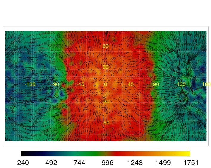
High in the atmosphere, there is a strong day-night temperature difference and wind speeds of several km s^-1 blow from day to night across the east terminator and over the poles (see Figure 1, top panel, at $\sim$2.5 mbar). As a rough measure of how quickly winds can move hot air from the dayside to the nightside, we calculate the advective timescale, $\tau_{\mathrm{adv}}=(\pi R_{p})/[u]_{\mathrm{eqtr}}$, where $R_{p}$ is the planet radius and $[u]_{\mathrm{eqtr}}$ is the zonal average of zonal wind at the equator. This advective timescale for east-west flow along the equator is generally faster than for the north-south flow. Above $\sim$200 mbar, the radiative timescales are less than the advective timescales and the temperature pattern is thus largely determined by the insolation, despite the supersonic km s^-1 winds.

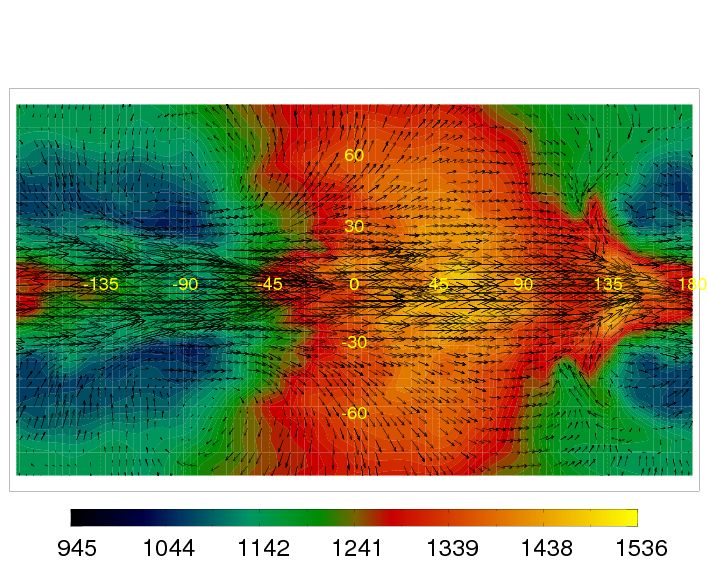
As the atmosphere transitions to having longitudinal advective timescales shorter than the radiative ones, there is significant advection of heated gas away from the substellar point, by $\sim$45^o to the east at $\sim$200 mbar. The winds are still supersonic, but now the flow is dominated by a super-rotating (eastward) equatorial jet, approximately extending from 30^o N to 30^o S in latitude (Figure 1, bottom panel, at $\sim$220 mbar). At high latitudes there are quasi-stationary vortices at the west terminator. Such vortices also exist in the shallower model of Menou & Rauscher (2009), although at a longitude of -135^o rather than -90^o like here. There is also a strongly convergent flow feature at a longitude of +135^o that we discuss in detail in §4.3.

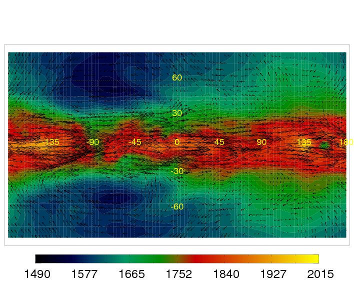
Below this level the advective timescales are much shorter than the radiative forcing times, the winds become subsonic, and the temperature pattern is more longitudinally homogenized. The equatorial jet, which has extended down through much of the atmosphere, ends at $\sim$4.4 bar (Figure 2, top panel). At this pressure level, vortices are found on the edges of the jet, as well as around the poles.

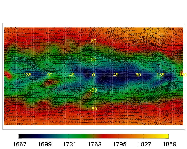
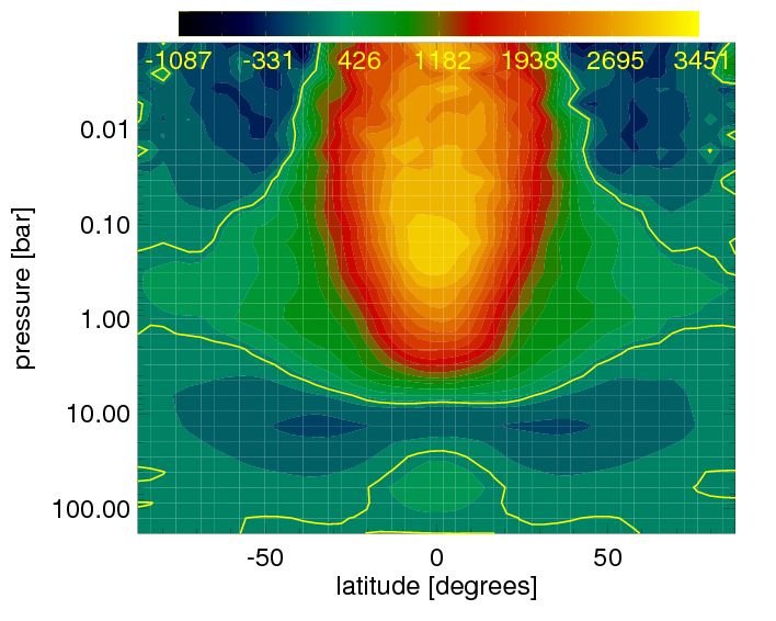
Below 10 bar the atmosphere is no longer heated by the stellar irradiation and the maximum wind speeds drop to several hundred m s^-1. The 20 bar level (Figure 2, bottom panel) is located below the main super-rotating jet (seen in Figure 1, bottom panel, and Figure 2, top panel) but also above another deeper, weaker, super-rotating jet (see Figure 3 below). The equatorial flow at 20 bar is retrograde (westward) and temperature increases with latitude, as expected from geostrophic balance with the anticyclonic flows around each pole.

3.2 Vertical structure

3.2.1 Wind profiles

For another view of how the flow structure changes throughout the atmosphere, we plot the zonal average of the zonal wind as a function of pressure and latitude, calculated as

$$[u(P,\phi)]\equiv\frac{1}{2\pi}\int_{0}^{2\pi}u(P,\lambda,\phi)\ d\lambda$$ (3)

where $u$ is the zonal (east-west) wind, $P$ is pressure, and $\phi$ and $\lambda$ are latitude and longitude. Figure 3 reveals the strong super-rotating jet that extends throughout most of the heated atmosphere (above 10 bar). The peak zonal wind speed in the jet occurs at the depth where the radiative and longitudinal advective timescales are roughly equal. The short radiative times in the upper atmosphere drive fast winds, but since the flow there is directed from day- to night-side across all regions of the terminator, the westward flow averages against the eastward flow. Thus the peak in the zonal wind speed occurs at a point of balance between absolute wind strength and zonal wind coherence, which is more clearly established at lower levels, where the flow is dominated by the eastward jet.

As shown in Fig. 3, the strongest westward flow at the equator occurs around 10 bar, as the atmosphere transitions from active to inert regions. The inert lower layers also develop a super-rotating jet, but it is much weaker than the one in the active layers. Although the mass of the atmosphere is dominated by the lowest levels, the region between 80 mbar - 6 bar contains $\sim 2/3$ of the total kinetic energy of the atmosphere, as we shall now see.

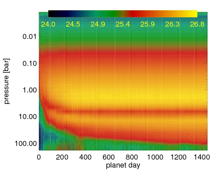
We plot the wind kinetic energy of each atmospheric layer as a function of time for the length of our run in Figure 4 to characterize the development of the modeled flow. The atmosphere begins at rest, but by planet day 1 supersonic winds have developed in layers above 150 mbar. By the end of the run the peak kinetic energy is located at $P\sim 2$ bar, but it takes about 300 planet days for these levels to fully adjust to the radiative forcing, where the local radiative timescales are relatively long ($\approx$ 5 planet days).

Below 10 bar, the atmosphere is not being driven by direct radiative forcing, but instead by transfer of heat and momentum from layers higher up. By the end of the run the layers below 10 bar have horizontal temperature variations of less than 100 K from their average values of $\sim$1800 K. Since these are small temperature differences, it seems that the main driver of the flow in the lower atmosphere would be momentum transport from above. This transport to deeper levels continues throughout the entire run and there is evidence that the lower levels have not reached a fully stationary state by the end of our run. We leave further discussion of concerns related to this issue until §4.2.

Lastly, we note the presence of some amount of horizontal kinetic energy associated with layers just above the model bottom boundary, especially early on, showing a quasi-oscillatory behavior. A run without initial surface pressure noise shows a similar behavior. We have not been able to unambiguously identify the origin of this flow feature, which may be related to some form of vertical propagation from the upper layers and subsequent interaction with the bottom boundary.

3.2.2 Temperature profiles

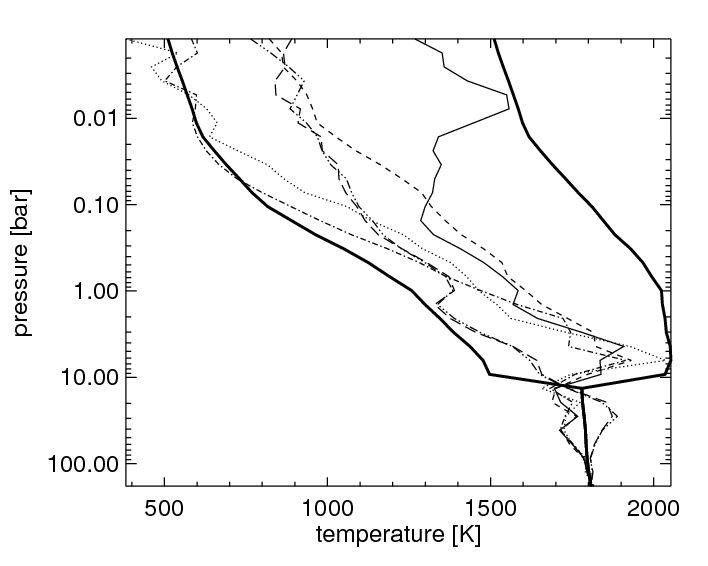
In addition to analyzing the variation of flow pattern with height, it is also worth considering the vertical temperature profiles around the planet. In Figure 5 we plot the variation of temperature with pressure for six representative locations: the sub- and antistellar points, the equator at the east and west terminators, and the north and south poles. Also shown are the radiative relaxation (forcing) profiles for the substellar point and everywhere on the nightside. Below 10 bar the atmosphere is not forced and instead we show an initial temperature profile for that region.

Interestingly, the profile at the substellar point contains a temperature inversion in the upper atmosphere. Our forcing profile is not inverted and so this inversion is due to dynamics alone. We note that this is not the first instance of a dynamically-induced temperature inversion in hot Jupiter atmospheric models, with inversions of similar magnitude found in Cooper & Showman (2006) and Showman et al. (2008a). However, given the growing observational evidence for temperature inversions on some hot Jupiters (Harrington et al., 2007; Knutson et al., 2008; Machalek et al., 2008; Knutson et al., 2009b), we find it worthwhile to emphasize that dynamics could play a role in creating such inversions. Radiative transfer models used to explain these observations generally invoke inversions that are much stronger than the one presented here (Burrows et al., 2008; Fortney et al., 2008), but it is possible that these models would not require as large an amount of absorbers as they do (e.g., Spiegel et al., 2009) if the role of dynamics in creating such inversions were included. Burrows et al. (2008) show that the presence of absorbing species are primarily responsible for the inversions, but advection of hot gas can play a secondary role.

Our terminator profiles at the east/west equator and the north/south poles are significantly hotter than if they were in local radiative equilibrium. The forcing profile, which defines local radiative equilibrium, is identical around the terminator and equal to the nightside profile shown in Figure 5. By comparison, we find atmospheric temperatures at the terminator which are hotter than the radiative equilibrium values by hundreds of Kelvin. Although the terminator relaxation profiles adopted in the present model cannot be considered as very realistic, a systematic bias toward hotter temperatures could have a significant impact on interpretations of transit spectroscopy observations (e.g., Sing et al., 2008; Swain et al., 2008b), especially since those measurements probe regions above $\sim$100 mbar, where we find the strongest deviations from radiative equilibrium.

Finally, an examination of vertical stability reveals that the nightside temperature profile, at the antistellar point, is convectively unstable across a few layers above the 40 mbar level. All of the other plotted profiles are stably stratified. Our code does not include any special treatment for convective columns and the occurrence of convection may thus introduce substantial errors in at least part of the modeled upper atmosphere. Convection acts as an efficient vertical mixing process and its occurrence in the upper atmosphere could facilitate the transport of minor absorbers, with possible consequences for the radiative transfer and the overall structure of the upper atmosphere (e.g., Spiegel et al., 2009). An adequate treatment of convective columns may thus be needed in future hot Jupiter atmospheric models although we note that Showman et al. (2009) do no report any convective columns in more advanced models with explicit non-gray radiative transfer.

4 Discussion

Our flow can be generally characterized as having an upper atmosphere dominated by radiative forcing, a transition to an advection-dominated regime at lower levels, and a low level of variability. This agrees at a basic level with the results of C&S, but we find several interesting differences that reveal possible areas of concern for future modeling efforts. We compare our results with C&S in detail in §4.1 and discuss possible reasons for these differences. In §4.2 and §4.3 we emphasize concerns related to vertical exchange between layers in the atmosphere and the presence of a shock-like feature.

4.1 Comparison with the work of Cooper & Showman

It is reassuring that our results agree at a basic level with those of C&S since they both are the consequence of the same set of physical equations applied to essentially identical conditions. The pressure levels plotted in Figure 1 of Cooper & Showman (2005) correspond to the levels shown in our Figure 1, top and bottom, and Figure 2, bottom. The top two levels show similar temperature and flow patterns, as well as matching maximum (supersonic) wind speeds. Points of interest are exactly where the models differ, as these indicate where our methods of solution for these equations may break down in the hot Jupiter regime.

First, however, we should focus on the greatest difference in set up between our model and that of C&S: the lower boundary. The model of C&S reaches down to 3 kbar while we only descend to 220 bar. This may be the main cause of differences between our 20 bar level flow (Figure 2, bottom panel) and that of Cooper & Showman (2005), shown in their Figure 1c. Our super-rotating equatorial jet descends to $\sim$7 bar whereas theirs reaches below 50 bar (compare our Figure 3 with Showman & Cooper, 2006, Fig. 2). In addition, their zonal profile shows a sharp distinction between the upper layers, where the flow is almost completely eastward, and the westward flow in the lower layers. In contrast, we find flow in both directions in our active layers. We partly attribute these differences in zonal flow to the extra momentum available from the deeper reservoir of inert layers in C&S. Since the simulation begins with no winds, the net angular momentum of the atmosphere must remain at the value set by the bulk planetary rotation at all times. For a deep eastward jet to form, the positive excess momentum must be balanced by a westward flow elsewhere in the atmosphere. The deepest model levels develop such a momentum balancing flow. In support of this interpretation, we note that our test run without any layers below 10 bar achieved a very similar flow in the upper layers while the eastward jet was constrained to terminate somewhat higher up in the atmosphere. We discuss the issue of vertical transport of momentum in more detail in the next section (4.2), but here we simply note that our fiducial model and the one without inert layers show good agreement except in the lowest model levels, suggesting that the difference in bottom boundary between our model and C&S does not strongly influence the modeled upper atmospheric flow.

Our next major difference with C&S is that our model contains significantly more detailed flow features, including vortices, especially at levels below 100 mbar. Since the large vortices in our model tend to extend all the way up to the poles (Figure 1, bottom panel) or flow around the poles (Figure 2), their absence in the work of C&S could be related to the traditional difficulty in treating the polar regions in a grid-based code. In fact, we note that the more recent work by Showman et al. (2009), which uses a cubed-sphere grid designed to address this polar issue specifically, contain “gyres” that extend up to high latitudes and may be analogous to the large scale vortices in our model.

The dynamical scales for jets and vortices on hot Jupiters are expected to be comparable to the planetary radius (Showman & Guillot, 2002; Menou et al., 2003). Showman et al. (2008a) have argued that the horizontal resolution in a model like ours or that in C&S should be sufficient to resolve the important atmospheric dynamical features. The model presented in Showman et al. (2008a) improves upon C&S by using relaxation temperature profiles calculated from one dimensional radiative transfer models for 14 insolation angles away from the substellar point, values of $\tau_{\mathrm{rad}}$ which depend on pressure and temperature, and twice the horizontal resolution. The flow pattern in their model of HD 209458b (shown in their Figure 5) more closely resembles our results than C&S in several ways, especially regarding the presence of a shock-like feature in the equatorial region around longitude +145^o E. We note that runs at twice the horizontal or vertical resolution produced very similar results, with only modest differences at the deepest model levels.

The emergence of sharp shock-like features in hot Jupiter atmospheres may have a significant impact on the nature of the atmospheric flow, as discussed in more detail in §4.3, but it may also lead to noticeable differences between models using different methods of solution, such as our model and that of C&S. Let us consider the issue of hyperdissipation as a specific example. In order to model the effect of dissipation on subgrid scales, atmospheric circulation models include an artificial term that works to damp features at the smallest resolved scales (e.g., Stephenson, 1994). C&S make use of a fourth-order hyperdiffusion term operating on the velocity field, $dv/dt\propto-\kappa\nabla^{4}v$, where $\kappa$ is a coefficient adjusted to dissipate the smallest model scales on a timescale of $\sim 30$ minutes. On the other hand, eighth-order hyperdissipation terms in our model act on the divergence and relative vorticity flow fields, as represented in Equation (2), on a timescale of $\sim 130$ minutes. Both methods are meant to prevent the build up of noisy features on small scales, but they may also have the unintended consequence of diffusing small-scale shock-like features that develop in hot Jupiter model flows. Such distinction could introduce an important algorithmic difference between models, to the extent that applying a diffusion operator on the velocity or the divergence field of a narrow divergent/convergent shock-like feature is significant. While hyperdiffusion terms may not be treating such features correctly, as we discuss in §4.3, they may also treat them differently and this could cause some of the dissimilarities between our model results and those of C&S.

4.2 Vertical exchange

There is a discontinuity between active and inert layers in our model and that of C&S, with a sudden jump from long radiative timescales to infinitely large ones. A more realistic transition is used by Showman et al. (2008a), with radiative timescales continuously increasing down through the atmosphere, so that there is no clear distinction between active and inert layers. Even then, the bottom boundary of the model is located above the convective interior and the nature of the interaction between the upper radiative atmosphere and the inner convective planetary interior is left unspecified. Understanding the nature of vertical exchanges in the deep atmospheres of gaseous giant planets is of great interest, whether it concerns hot Jupiters or Solar System giants (e.g., Lian & Showman, 2008; Schneider & Liu, 2009).

Vertical exchange of momentum and heat between our active and inert layers is seen to occur, as discussed in §3.2. One consequence of this interaction is apparent in Figure 3, where the levels above 10 bar are dominated by an eastward flow (with net excess angular momentum), with a compensating westward flow in the deeper inert layers (with a net angular momentum deficit). The ability of the upper layers to acquire angular momentum from the lower levels allows for stronger eastward flow than would otherwise be possible, e.g., if the radiatively forced layers were isolated. In the absence of momentum forcing, a much shallower atmosphere would have to maintain this net angular momentum budget by balancing an eastward flow with a westward flow essentially within the same atmospheric layer. This situation appears to be realized in the shallow hot Jupiter model presented by Menou & Rauscher (2009), leading to the development of strong horizontal shear and barotropic instabilities. By contrast, vertical transport of angular momentum between layers can occur throughout a deep atmosphere. It connects the dynamics of the upper atmosphere with various interior processes, with possibly significant implications for a planet’s tidal evolution and cooling history (e.g., Guillot & Showman, 2002; Showman & Guillot, 2002).

When modeling the upper atmosphere, the main difficulty in correctly treating interaction with the deeper layers and the planetary interior comes from our ignorance of the physical processes involved, as well as issues of timescales. In the upper atmosphere, the timescales of interest are much shorter than those in the interior. In fact, layers below 10 bar in our model have not reached a stationary state by the end of the run, as shown in Figure 4. They continue to acquire kinetic energy from interaction with the radiatively forced region, although this does not seem to significantly affect the upper atmospheric flow itself. As mentioned earlier, we ran a test model excluding inert layers, i.e., with a model lower boundary set at 10 bar, and found significant differences only in the bottom few layers, with a stronger westward flow just above 10 bar. This suggests that the nature of the upper atmospheric flow is dominated by radiative forcing rather than by exchange with deeper layers but the issue of vertical exchange of heat and momentum in the deep atmospheres of hot Jupiters probably deserves further attention in the future.

4.3 The shock-like feature

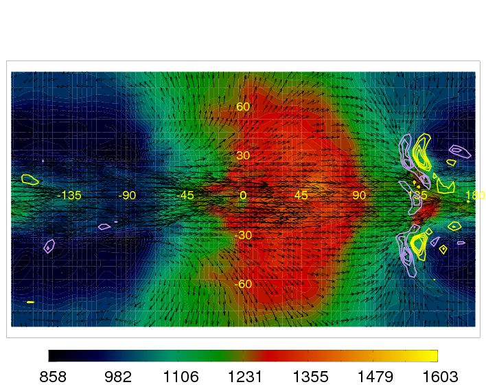
The bottom panel of Figure 1 shows the presence of a chevron-shaped feature in the 220 mbar temperature map, at longitude +135^o E. In Figure 6, we over-plot contours of horizontal flow convergence (and divergence) on a temperature and wind map one level higher in the atmosphere, at 150 mbar. There is a narrow region of strong horizontal flow convergence at the 150 mbar level which matches well the temperature feature seen at the same longitude, at the 220 mbar level, in Figure 1. We identify this flow feature as “shock-like” because unusually strong local flow convergence is a signature of hydrodynamical shocks. Our numerical solver does not include any special treatment of the shock physics, however. The feature extends vertically across a range of layers, with hints of it even as high as 2.5 mbar (Figure 1, top panel), but it is most apparent in levels from 50 - 150 mbar. The regions of strong horizontal convergence generally coincide with areas of higher temperatures for the atmospheric gas. Although we have not attempted a more detailed characterization of this flow feature, we note that it is consistent with adiabatic heating of a downward flow associated with horizontal convergence above (as discussed by Showman et al., 2009). The influence of this localized source of heating may extend rather deep into the atmosphere, so that the increased temperature region centered around longitude +135^o at the 4.4 bar level (Figure 2, top panel) may also be a consequence of the flow higher up, rather than being caused by horizontal advection of heat away from the substellar point.

Recently, Showman et al. (2009) reported a similar feature in their model of the hot Jupiter HD 189733b, which they identified as a hydraulic jump. Another such feature can be seen in their model for HD 209458b. In fact, a similar feature also seems to be present, but not commented upon, in the models of these same planets by Showman et al. (2008a). We note that the primitive equations of meteorology impose hydrostatic balance, which filters out vertically propagating sound waves. Horizontal sound waves, however, are permitted given appropriate boundary conditions (Kalnay, 2002; Vallis, 2006), so that finite amplitude waves of this nature (also known as Lamb waves) could presumably steepen into shocks. The partial-globe model of Dobbs-Dixon & Lin (2008) solves the full three dimensional Navier-Stokes equations and these authors also find a shock-like, chevron-shaped feature in their hot Jupiter model around +135^o longitude (see their Figure 6). Since shock-like features are present in models of increasing complexity (this work, Showman et al., 2008a, 2009), in a model that includes fully three dimensional sound waves (Dobbs-Dixon & Lin, 2008), and in models for different planets, it may be that the development of such features is a natural outcome of the hot Jupiter circulation regime. While the steepening of finite amplitude sound (or Lamb) waves is a possible path to the formation of shocks in an atmosphere with transonic wind speeds, the detailed nature of these shock-like features remains to be investigated and understood.

Most meteorological models are not designed to treat the three dimensional compressible nature of atmospheric flows or the formation of shocks because these are issues which are clearly subdominant in the context of Earth atmospheric modeling, with very subsonic wind speeds. Any model that assumes hydrostatic balance has filtered out vertically propagating sound waves, while the use of rigid top and bottom boundary conditions would exclude even horizontally propagating sound waves (i.e., Lamb waves; Kalnay, 2002). In meteorological models that do admit horizontal sound waves, there usually is no explicit treatment of shock physics, so that shocks would be subject to ill-constrained conditions on the smallest resolved model scales (see also the discussion of hyperdiffusion in §4.1). Physically, the dissipation of bulk kinetic energy in a shock, and its conversion to localized heating, could have a substantial impact on the flow, and one that cannot be easily estimated without an explicit treatment of shocks. Goodman (2009) clearly emphasizes various concerns regarding this issue. Future hot Jupiter models may thus need to include shock-capturing schemes to more faithfully describe this aspect of their new circulation regime.

5 Summary and Conclusions

It is reassuring to find a basic level of consistency between our work and that of C&S. In fact, the general agreement between our hot Jupiter model and more complex versions described by Showman et al. (2008a, 2009) seems to indicate that some of the basic attributes of the circulation regime in hot Jupiter atmospheres has been successfully captured. Nevertheless, significant discrepancies also emerge from our direct comparison with the work of C&S. These discrepancies could have their origin in the different methods of solution adopted and/or the fact the equations solved are missing some of the physics at work in the hot Jupiter context.

Meteorological solvers like our pseudo-spectral IGCM and the grid-based code used by C&S have been successfully compared to each other in the context of Earth atmospheric modeling (Held & Suarez, 1994). They very accurately solve the equations of meteorology and produce fully consistent results, which are also in agreement with the known general circulation regime on Earth. In the hot Jupiter modeling context, we cannot be certain of the accuracy and validity of these models until they can likewise produce consistent results. The discrepancies identified here between our model results and those of C&S suggest that one or both numerical solvers do not faithfully capture all of the atmospheric physics at work in the hot Jupiter context. Areas of specific concern for future hot Jupiter atmospheric modeling include the following.

• The interaction between the radiatively forced upper atmosphere, deeper atmospheric layers, and the convective planetary interior. Although the upper atmosphere seems to be rather weakly sensitive to the lower boundary condition on the relatively short timescales described by our model (hundreds of planet days), the nature of heat and momentum exchanges between the modeled atmosphere and the unmodeled planetary interior could be a significant source of uncertainties for hot Jupiter models.

• Dissipation of bulk kinetic energy and conversion to localized heating in shock-like features. Explicit treatment of this energy conversion process may have a first order effect on the flow thermodynamics, as emphasized by Goodman (2009). Previous atmospheric models, in circulation regimes with typically subsonic wind speeds, did not have to treat such shock-like features.

• Convection. If atmospheric columns are found to be convective in hot Jupiter models with more advanced treatments of radiative transfer and atmospheric chemistry, it will be necessary to implement convective adjustment schemes to properly describe the rapid vertical mixing of entropy and momentum. Vertical mixing of radiatively active species could also have important consequences for the atmospheric structure.

Finally, our hot Jupiter model results also inform some of the current efforts focused on the interpretation of a growing set of hot Jupiter observational data. We have emphasized the possibility that atmospheric dynamics alone could produce upper atmospheric temperature inversions, albeit not necessarily of the strength typically required to explain observed hot Jupiter secondary eclipse spectra. Nevertheless, it may be important to recognize the role of dynamics in this phenomenon. In addition, we have found that temperature profiles along the terminator in our model upper atmosphere are systematically raised above the local radiative equilibrium values. This is a potential source of bias for interpretations of transmission spectra which often rely on the assumption of temperature profiles in radiative equilibrium.

Figure 1: Temperature (in K) and wind maps at pressure levels of 2.5 mbar (top) and 220 mbar (bottom) in our hot Jupiter model. Each map is shown in Miller cylindrical projection, with the substellar point located at (0,0). The maximum wind speeds are 10 (top) and 4 km s^-1(bottom). High in the atmosphere, winds are very strong and directed away from the dayside, but the temperature pattern remains strongly determined by insolation. Somewhat deeper in the atmosphere, the winds become more efficient at advecting hot gas away from the dayside before it cools significantly. A strong super-rotating equatorial jet develops.

Figure 2: Temperature (in K) and wind maps, continued from Figure 1, at pressure levels of 4.4 bar (top) and 20 bar (bottom) in our hot Jupiter model. Maximum wind speeds are 1 (top) and 0.2 km s^-1(bottom). At these deeper levels, the winds have largely homogenized the longitudinal temperature structure, although some latitudinal gradient remains. The super-rotating equatorial jet descends through much of the atmosphere, down to approximately 7 bar.

Figure 3: Zonal average of the zonal wind in m s^-1, as a function of latitude and depth in the atmosphere. Yellow lines separate regions of positive (eastward) flow and negative (westward) flow. A strong super-rotating equatorial jet descends through much of the atmosphere. At the equator the maximum (eastward) zonal-average wind speed occurs where the radiative and advective timescales are comparable. Deep in the atmosphere, the minimum (peak westward) zonal-average wind speed occurs at the transition between radiatively forced and inert layers.

Figure 4: Logarithm (log₁₀) of the total wind kinetic energy (in joules) in each layer of the model atmosphere as a function of atmospheric depth and planet day in the run. The kinetic energy at each level is calculated as the horizontal integral of $\rho v_{H}^{2}/2$, where $\rho$ is the density and $v_{H}$ is the horizontal wind speed. The atmosphere starts at rest but it quickly develops a transonic flow. The equatorial jet shown in Figure 3 contains most of the kinetic energy of the atmosphere. The inert layers below 10 bar slowly gain kinetic energy by exchange with the radiatively forced layers above, and they have yet to reach a stationary state by the end of the run.

Figure 5: Temperature-pressure profiles at six points around the planet: the substellar point (thin solid), the antistellar point (dotted), the equator at the east terminator (dashed), the equator at the west terminator (dot-dashed), the north pole (triple dot-dashed), and the south pole (long dashed). The thick solid lines show the radiative relaxation (forcing) temperature profiles at the substellar point and on the nightside above 10 bar, as well as the initial temperature profiles below 10 bar (where there is no radiative forcing by construction). Note the presence of a dynamically-induced temperature inversion (“stratosphere”) at the substellar point and significant deviations from radiative equilibrium all around the limb.

Figure 6: Contours of horizontal flow convergence (in lavender) and divergence (in yellow) plotted over the temperature (in K) and wind map at the 150 mbar pressure level. The convergence/divergence contour levels are set at $\pm 1\times 10^{-4}$, $1.5\times 10^{-4}$, $2\times 10^{-4}$, and $2.5\times 10^{-4}$ s^-1. Clearly, the bulk of the flow has $|\nabla\cdot\mathbf{v}|<1\times 10^{-4}$ s^-1. The narrow region of strong convergence around longitude +135^o is what we refer to as a shock-like feature. An increase in temperature around longitude +135^o seen in the bottom panel of Figure 1, just one model level below the one shown here, is consistent with adiabatic heating by a downward flow associated with this shock-like feature.

References

- Agol et al. (2009) Agol, E., Cowan, N. B., Bushong, J., Knutson, H., Charbonneau, D., Deming, D., & Steffen, J. H. 2009, IAU Symposium, 253, 209
- Burkert et al. (2005) Burkert, A., Lin, D. N. C., Bodenheimer, P. H., Jones, C. A., & Yorke, H. W. 2005, ApJ, 618, 512
- Burrows et al. (2008) Burrows, A., Budaj, J., & Hubeny, I. 2008, ApJ, 678, 1436
- Charbonneau et al. (2005) Charbonneau, D., et al. 2005, ApJ, 626, 523
- Charbonneau et al. (2002) Charbonneau, D., Brown, T. M., Noyes, R. W., & Gilliland, R. L. 2002, ApJ, 568, 377
- Charbonneau et al. (2008) Charbonneau, D., Knutson, H. A., Barman, T., Allen, L. E., Mayor, M., Megeath, S. T., Queloz, D., & Udry, S. 2008, ApJ, 686, 1341
- Cho et al. (2003) Cho, J. Y.-K., Menou, K., Hansen, B. M. S., & Seager, S. 2003, ApJ, 587, L117
- Cho et al. (2008) Cho, J. Y.-K., Menou, K., Hansen, B. M. S., & Seager, S. 2008, ApJ, 675, 817
- Cooper & Showman (2005) Cooper, C. S., & Showman, A. P. 2005, ApJ, 629, L45 (C&S)
- Cooper & Showman (2006) Cooper, C. S., & Showman, A. P. 2006, ApJ, 649, 1048
- Cowan et al. (2007) Cowan, N. B., Agol, E., & Charbonneau, D. 2007, MNRAS, 552
- Deming et al. (2007) Deming, D., Harrington, J., Laughlin, G., Seager, S., Navarro, S. B., Bowman, W. C., & Horning, K. 2007, ApJ, 667, L199
- Deming et al. (2005) Deming, D., Seager, S., Richardson, L. J., & Harrington, J. 2005, Nature, 434, 740
- Demory et al. (2007) Demory, B.-O., et al. 2007, A&A, 475, 1125
- Dobbs-Dixon & Lin (2008) Dobbs-Dixon, I., & Lin, D. N. C. 2008, ApJ, 673, 513
- Fortney et al. (2008) Fortney, J. J., Lodders, K., Marley, M. S., & Freedman, R. S. 2008, ApJ, 678, 1419
- Goodman (2009) Goodman, J. 2009, ApJ, 693, 1645
- Grillmair et al. (2007) Grillmair, C. J., Charbonneau, D., Burrows, A., Armus, L., Stauffer, J., Meadows, V., Van Cleve, J., & Levine, D. 2007, ApJ, 658, L115
- Guillot & Showman (2002) Guillot, T., & Showman, A. P. 2002, A&A, 385, 156
- Harrington et al. (2006) Harrington, J. et al. 2006, Science, 314, 623
- Harrington et al. (2007) Harrington, J., Luszcz, S., Seager, S., Deming, D., & Richardson, L. J. 2007, Nature, 447, 691
- Held & Suarez (1994) Held, I. M., & Suarez, M. J. 1994, Bulletin of the American Meteorological Society, 75, 1825
- Hoskins & Simmons (1975) Hoskins, B. J., & Simmons, A. J. 1975, Quarterly Journal of the Royal Meteorological Society, 101, 637
- Iro et al. (2005) Iro, N., Bezard, B. & Guillot, T 2005, A&A, 436, 719
- Kalnay (2002) Kalnay, E. 2002, Atmospheric Modeling, Data Assimilation and Predictability, by Eugenia Kalnay, pp. 364. ISBN 0521791790. Cambridge, UK: Cambridge University Press, December 2002
- Knutson et al. (2007) Knutson, H. A., et al. 2007, Nature, 447, 183
- Knutson et al. (2009a) Knutson, H. A., et al. 2009a, ApJ, 690, 822
- Knutson et al. (2008) Knutson, H. A., Charbonneau, D., Allen, L. E., Burrows, A., & Megeath, S. T. 2008, ApJ, 673, 526
- Knutson et al. (2009b) Knutson, H. A., Charbonneau, D., Burrows, A., O’Donovan, F. T., & Mandushev, G. 2009b, ApJ, 691, 866
- Kundu & Cohen (2004) Kundu, P. K. & Cohen, I. M. 2004, Fluid Mechanics: Third Edition. Published by Academic Press, Elsevier, Inc., London, England.
- Langton & Laughlin (2007) Langton, J., & Laughlin, G. 2007, ApJ, 657, L113
- Laughlin et al. (2009) Laughlin, G., Deming, D., Langton, J., Kasen, D., Vogt, S., Butler, P., Rivera, E., & Meschiari, S. 2009, Nature, 457, 562
- Lian & Showman (2008) Lian, Y. & Showman, A. P. 2008, Icarus 195, 597
- Machalek et al. (2008) Machalek, P., McCullough, P. R., Burke, C. J., Valenti, J. A., Burrows, A., & Hora, J. L. 2008, ApJ, 684, 1427
- Menou et al. (2003) Menou, K., Cho, J. Y.-K., Seager, S., & Hansen, B. M. S. 2003, ApJ, 587, L113
- Menou & Rauscher (2009) Menou, K., & Rauscher, E. 2009, ApJ, 700, 887
- Pont et al. (2008) Pont, F., Knutson, H., Gilliland, R. L., Moutou, C., & Charbonneau, D. 2008, MNRAS, 385, 109
- Richardson et al. (2007) Richardson, L. J., Deming, D., Horning, K., Seager, S., & Harrington, J. 2007, Nature, 445, 892
- Schneider & Liu (2009) Schneider, T. & Liu, J. 2009, J. Atmos. Sci. 66, 579
- Showman & Cooper (2006) Showman, A. P., & Cooper, C. S. 2006, Tenth Anniversary of 51 Peg-b: Status of and prospects for hot Jupiter studies, 242, arXiv:0705.2836v1
- Showman et al. (2008a) Showman, A. P., Cooper, C. S., Fortney, J. J., & Marley, M. S. 2008a, ApJ, 682, 559
- Showman et al. (2009) Showman, A. P., Fortney, J. J., Lian, Y., Marley, M. S., Freedman, R. S., Knutson, H. A., & Charbonneau, D. 2009, ApJ, 699, 564
- Showman & Guillot (2002) Showman, A. P. & Guillot, T. 2002, A&A, 385, 166
- Showman et al. (2008b) Showman, A. P., Menou, K., & Cho, J. Y.-K. 2008b, Astronomical Society of the Pacific Conference Series, 398, 419
- Sing et al. (2008) Sing, D. K., Vidal-Madjar, A., Lecavelier des Etangs, A., Désert, J.-M., Ballester, G., & Ehrenreich, D. 2008, ApJ, 686, 667
- Spiegel et al. (2009) Spiegel, D. S., Silverio, K., & Burrows, A. 2009, arXiv:0902.3995
- Stephenson (1994) Stephenson, D. B. 1994, Q. J. R. Meteo. Soc. 120, 211
- Suarez & Takacs (1995) Suarez, M. J., & Takacs, L. L. 1995, Documentation of the ARIES/GEOS Dynamical Core, ver. 2 (NASA Tech. Memo 104606, Vol. 5; Greenbelt: GSFC)
- Swain et al. (2008a) Swain, M. R., Bouwman, J., Akeson, R. L., Lawler, S., & Beichman, C. A. 2008a, ApJ, 674, 482
- Swain et al. (2008b) Swain, M. R., Vasisht, G., & Tinetti, G. 2008b, Nature, 452, 329
- Tinetti et al. (2007) Tinetti, G., et al. 2007, Nature, 448, 169
- Vallis (2006) Vallis, G.K. 2006, ’Atmospheric and Oceanic Fluid Dynamics’ (Cambridge University Press)