Understanding interference experiments with polarized light through photon trajectories
Abstract
Bohmian mechanics allows to visualize and understand the quantum-mechanical behavior of massive particles in terms of trajectories. As shown by Bialynicki-Birula, Electromagnetism also admits a hydrodynamical formulation when the existence of a wave function for photons (properly defined) is assumed. This formulation thus provides an alternative interpretation of optical phenomena in terms of photon trajectories, whose flow yields a pictorial view of the evolution of the electromagnetic energy density in configuration space. This trajectory-based theoretical framework is considered here to study and analyze the outcome from Young-type diffraction experiments within the context of the Arago-Fresnel laws. More specifically, photon trajectories in the region behind the two slits are obtained in the case where the slits are illuminated by a polarized monochromatic plane wave. Expressions to determine electromagnetic energy flow lines and photon trajectories within this scenario are provided, as well as a procedure to compute them in the particular case of gratings totally transparent inside the slits and completely absorbing outside them. As is shown, the electromagnetic energy flow lines obtained allow to monitor at each point of space the behavior of the electromagnetic energy flow and, therefore, to evaluate the effects caused on it by the presence (right behind each slit) of polarizers with the same or different polarization axes. This leads to a trajectory-based picture of the Arago-Fresnel laws for the interference of polarized light.
keywords:
Maxwell equations , Photon wave function , Hydrodynamic formulation of Electromagnetism , Electromagnetic energy flow line , Photon trajectory , Bohmian mechanics , Quantum trajectoryPACS:
03.50.De , 42.50.-p , 42.50.Ar , 03.65.Ta , 42.25.Hz , 42.25.Ja1 Introduction
By means of different experimental techniques based on the use of low-intensity beams, nowadays it is possible to observe the gradual emergence of interference patterns in the case of both massive particles [1, 2] and light (photons) [3, 4, 5]. That is, the patterns are built up by detecting single events (one by one) which can be followed on a screen as a function of time. In the pattern formation sequence, at short time scales, when the number of events (or detections) recorded is still relatively low, seemingly random distribution of points can be observed on a screen used to monitor the experiment. However, as time proceeds and the number of detections increases sufficiently, the well-known band structure of alternate light and dark interference fringes starts to appear. Hence, moving from the darker regions of the pattern to the lighter ones means that the density of particles detected increases. This kind of experiments constitutes a nice manifestation of the statistical nature of Quantum Mechanics, which, in the large count-number limit, establishes that both massive particles [6] and photons [7] distribute according to a certain probability density.
Based on this kind of experiments, one could assume that each point on the screen corresponds to the final position of the trajectory pursued by a detected particle. This immediately leads to considering trajectory-based formulations to explain interference processes, where the analysis of the properties displayed by (particle) trajectories provides a dynamical explanation and interpretation of the process. In other words, these formulations would contain the mechanisms that allow to account for the appearance of fringes in interference experiments with quantum particles (either massive particles or photons) in the large-number limit of single-event counts, this outcome being in agreement with the results obtained from standard wave-based formulations. This is an important and remarkable advantage, for these approaches thus constitute physical models where both corpuscular and wave-like properties are compatible.
In the case of interference experiments with massive particles, different trajectory-based studies can be found in the literature [8, 9, 10, 11, 12, 13, 14, 15, 16], which are aimed to establish a bridge between the single counts observed experimentally and the statistical quantum-mechanical description in terms of smooth, continuous probability densities. Many of them rely on Bohmian mechanics [17, 18, 19, 20, 21], a hydrodynamic formulation of Quantum Mechanics in terms of trajectories, which, to some extent, can be considered at the same level as Newtonian mechanics with respect to (classical) Liouvillian mechanics. Bohmian trajectories evolve following the streamlines associated with the quantum probability current density (quantum flow) and, therefore, reproduce exactly the quantum-mechanical probability distribution in both the near and the far field when a large number of them is considered, in particular, in interference experiments [9, 10, 14]. Alternatively, the emergence of interference patterns in the far field has also been simulated by using trajectories determined from the momentum distribution (MD trajectories) associated with the particle wave function [16].
In the case of interference processes with light (photons), similar descriptions are not so numerous. Some early attempts to explain interference and diffraction in terms of electromagnetic energy (EME) flow lines were those of Braunbek and Laukien [22] and Prosser [23, 24]. Within this approach, based on Maxwell’s equations, the photon trajectories are associated with the EME flow lines [24], which are obtained after solving a trajectory equation arising from the Poynting energy flow vector [25]. Similarly, but starting from the Dirac equation instead of Maxwell’s ones, Ghose et al. [26] also determined photon trajectories. The formal grounds of these approaches are similar to those of the hydrodynamic formulation of Electromagnetism developed by Bialynicki-Birula [27, 28, 29, 30]. This formalism arises after assuming that, as happens with massive particles, photons can also be described by a well-defined wave function, this being a problem which has received much attention in the literature [27, 28, 29, 30, 31, 32, 33, 34, 35, 36, 37, 38, 39, 40, 41, 42]. Specifically, by following the same argumentation that led Dirac to the relativistic equation for the electron, Bialynicki-Birula [27, 28, 29, 30] reaches Maxwell’s equations. Accordingly, though these equations have a purely classical origin, they can be expressed as a Dirac-like equation, with the wave function satisfying it being a complex vector encompassing both the electric and magnetic field, namely the Riemann-Silberstein [43, 44] (see Appendix A).
More specifically, in order to better understand the relationship between EME flow lines and photons, consider the following. As mentioned above, the EME flow lines describe the paths along which the EME flows. Assuming that a wave function defined in terms of the EM field can be associated to a quantum of energy or photon [27, 28, 29, 30, 31, 32, 33, 34, 35, 36, 37, 38, 39, 40, 41, 42], the probability that a photon arrives at a certain region on a screen will be proportional to the EME density at that region, i.e., to the density of flow lines reaching such a region. Hence, one could interpret that the trajectory arrivals somehow simulate the arrivals of single photons to the screen, as seen experimentally [4, 5]. That is, the trajectories are the paths along which the EME flows and ensembles of them will constitute the eventual/possible paths taken by single photons. However, a photon itself has to be represented by an ensemble of trajectories in order to satisfy the condition of energy quantization. Throughout this work, we are going to use the term “photon trajectory” to denote any of the eventual EME flow lines or trajectories that a photon can pursue, but taking into account the previous discussion.
Recently, we have considered [45] Prosser’s approach (a simplified view of the more general Bialynicki-Birula hydrodynamical formulation) to study Young’s experiment and the Talbot effect for a monochromatic, linearly polarized incident electromagnetic (EM) field (or wave) reaching the diffracting grating. This study was carried out in the region between the grating (behind it) and the detection screen, thus the photon trajectories were computed directly from the diffracted wave function, which was obtained by requiring that the components of both the electric and the magnetic vector fields satisfied Maxwell’s equations as well as the boundary conditions imposed by the grating. The trajectories obtained showed how the EME redistributes in space from the grating to the detection screen, located far away from the former in the Fraunhofer region [9, 10]. By properly sampling the field at the slits, one could also observe how, as time proceeds, the accumulation of trajectory arrivals, which eventually led to the appearance of the well-known fringe-like pattern, just as in the analogous real experiment [3, 4, 5] or as in Quantum Mechanics, where the formation of similar patterns arises after a large count of particle trajectories.
In this work, we go a step forward and present a more general trajectory-based analysis of Young-type experiments carried out with polarized light. Experiments with high-intensity polarized beams are well-known since the beginning of the XIXth century, when Arago and Fresnel enunciated their laws for Young’s interference experiment with polarized light [46]. According to these laws, no interference pattern is observed if, for example, the two interfering beams are linearly polarized in orthogonal directions [47] or both are elliptically polarized but with opposite handedness [48]. By means of the Bialynicki-Birula hydrodynamical formulation of Electromagnetism [27, 28, 29, 30], here we provide a trajectory picture for this kind of experiments. Since we are interested in the interference phenomenon and its relationship with the polarization of the interfering waves, we start the calculation of the photon trajectories behind the slits. By assuming that the incoming wave is a polarized monochromatic EM plane wave, the components of the electric and magnetic fields can be expressed in terms of a function that explicitly takes into account the boundary conditions imposed by the two slits (here, the grating is considered to be totally transparent inside the slits and completely absorbing outside them). Within this scenario, we provide expressions to determine the photon trajectories as well as a procedure to compute them in the particular case of gratings totally transparent inside the slits and completely absorbing outside them. As is shown, the photon trajectories obtained allow to monitor at each point of space the behavior of the electromagnetic energy flow and, therefore, to evaluate the effects caused on it by the presence (right behind each slit) of polarizers with the same or different polarization axes. This thus constitutes a very interesting pictorial view of the Arago-Fresnel laws for the interference of polarized light, consistent with the more conventional one based on standard Electromagnetism.
The organization of this paper is as follows. In order to be self-contained, in Section 2 we introduce some fundamental theoretical grounds related to the photon-trajectory formalism, starting from Maxwell’s equation, as also done within the framework of the Bialynicki-Birula hydrodynamical formulation of Electromagnetism. Particularly, we will focus on those elements related to the analysis of experiments with polarized light. In Section 3, we describe the incident EM field and its polarization, as well as the derivation of the corresponding photon trajectories before reaching the interference grating. In Section 4, the EM field at and behind the grating is obtained as a solution of Maxwell’s equations. This field is going to be used to calculate later the associated photon trajectories. In Section 5, we present and discuss the photon trajectories behind a two-slit grating in the case of an incident circularly polarized EM field. In Section 6 an analogous analysis is carried out, but when the slits are covered with polarizers with orthogonal polarization axes. Calculations of photon trajectories for the cases of incident linearly and circularly polarized EM fields are shown. Finally, in Section 7 the conclusions arisen from this work are summarized.
2 Maxwell’s equations, EME flow lines and photon trajectories
Consider a monochromatic EM field propagating in vacuum. Under these conditions, the electric and magnetic components of this field can be expressed as harmonic waves, as
| (1) |
respectively, where the space dependent parts of these fields satisfy the time-independent Maxwell’s equations,
| (2) | |||||
| (3) | |||||
| (4) | |||||
| (5) |
as well as the boundary conditions associated with the particular problem under study. Equivalently, from (2)-(5), it is readily shown that both and satisfy the Helmholtz equation,
| (6) | |||
| (7) |
where .
The EME flow lines are obtained from the real part of the time-averaged complex Poynting vector [25],
| (8) |
as follows. We know that this vector describes the flow of the time-averaged EME density through space,
| (9) |
That is, the EME density is transported through space as a flow described by . Formally, this can be expressed as
| (10) |
where is a local effective velocity vector field, namely the ray velocity [49]. This velocity indicates the direction of the EME flow at each space point and its magnitude is equal to the EME that crosses in unit time an area perpendicular to the flow direction (given by the Poynting vector ) divided by the EME per unit volume. Taking into account the Bialynicki-Birula hydrodynamical viewpoint, one can assume that the EME travels along streamlines defined by (10). Therefore, this equation can be recast in a more convenient way as
| (11) |
whose solutions, , are the streamlines or EME flow lines followed by the EME density in configuration space or, within a Bohmian-like reinterpretation of the Bialynicki-Birula hydrodynamical formulation, the photon trajectories. Here, is simply a parameter which labels the evolution across space of the corresponding trajectory, however, for practical purposes, later we will reparametrize the solutions in terms of one of the coordinates —in particular, we consider the reparametrization .
In the particular case of interference experiments, a functional form for (11) can be found by means of the following considerations. The screen containing the grating is on the plane, at , and the slits are parallel to the -axis, their width () being much larger along this direction than along the -direction (i.e., ). Accordingly, we can assume that the EME density is independent of the -coordinate and, therefore, the electric and magnetic fields will not depend either on this coordinate. This allows us to consider a simplification in the analytical treatment, for, as mentioned in [49], a problem independent of one Cartesian coordinate is essentially scalar and, therefore, can be formulated in terms of one dependent variable. Thus, if we introduce here
| (12) |
into Eqs. (4) and (5), we obtain two independent sets of equations,
| (13) |
and
| (14) |
The set (13) only involves , and , and therefore is commonly referred as a case of -polarization, while the set (14), which only involves , and , is referred to as -polarization.
More specifically, as infers from the set of equations (13), in the case of -polarization the electric field is polarized along the -direction, while the magnetic field is confined to the plane . That is, , with the components of the magnetic field satisfying
| (15) |
Substituting these expressions for and into the second line of (13) yields
| (16) |
We thus have
| (17) | |||||
| (18) |
with satisfying Helmholtz’s equation, according to (16). Analogously, in the case of -polarization the magnetic field is polarized along the -direction and the electric one confined to the plane (i.e., ), with the components of the latter being
| (19) |
Substituting now these relations into the second line of (14) yields
| (20) |
which allows us to characterize -polarization as
| (21) | |||||
| (22) |
with satisfying the Helmholtz equation (20). Therefore, any general (time-independent) solution will be expressible as
| (23) | |||||
| (24) |
Since and satisfy Helmholtz’s equation, consider now that both are proportional to a scalar field, , which also satisfies this equation, i.e.,
| (25) | |||||
| (26) |
Here, and are real quantities and the phase shift between both components is given by ; (5) has been used to obtain the correct dimensionality in the r.h.s. of (26). If (25) and (26) are substituted into Eqs. (23) and (24), respectively, the latter become
| (27) | |||||
| (28) |
with their time-dependent counterparts being
Equations (LABEL:eq31) and (LABEL:eq32) are general time-dependent solutions for a problem which can be described in terms of superpositions, as also happens with (23) and (24). Once this set of equations is set up, the whole problem reduces to finding and its propagation along and (by the above hypothesis, the set of equations does not depend on ), which is a boundary condition problem.
3 Incident EM plane wave, its polarization and photon trajectories
Before reaching the two slits, we assume that both the electric and magnetic fields propagate along the -direction. Moreover, we also assume that the incident scalar field is a monochromatic plane wave,
| (31) |
Of course, this is just a simplification in order to develop some analytical expressions, where we have assumed that the incident wave is locally plane in a region that will cover the two slits. However, in a more realistic case, one could consider a more general incident wave function of a limited extension, like a beam or a wave packet. In the case of massive particles, the effects associated with incident wave functions of limited extension in two-slit experiments have been studied in [11, 12] (similarly, a study of the effects of the outgoing diffracted waves can be found in [10]).
Introducing (31) into (LABEL:eq31) and (LABEL:eq32) yields
| (32) | |||||
| (33) | |||||
From these solutions, it follows that the polarization is going to play an important role in the interference patterns observed, and also in the topology displayed by the photon trajectories.
Consider the electric field (32), whose real components are
| (34) | |||||
| (35) |
Since the magnetic field displays the same polarization properties as the electric field due to their relationship through the Maxwell equations (4) and (5), we will only argue in terms of the electric field without loss of generality. Thus, expressing (34) and (35) as
| (36) | |||||
| (37) |
and then squaring and rearranging terms, we reach
| (38) |
According to this relation, several cases are possible depending on the value of the phase-shift :
-
(a)
When or ,
(39) This case describes linear polarization, for any arbitrary and .
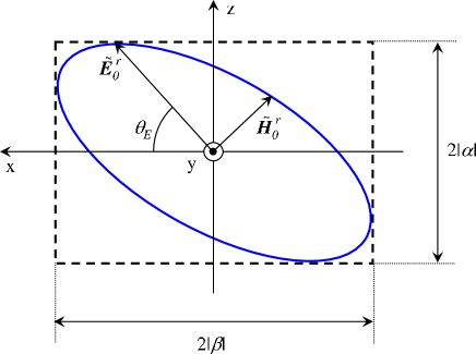
Figure 1: Diagram showing the general elliptic motion described by the electric field due to its polarization (the same applies to the magnetic field, which is perpendicular). If and , the ellipse becomes a circle (circular polarization), and if or , it reduces to a segment (linear polarization) regardless of the and values. -
(b)
For any other value of , there is elliptic polarization. In this case, (38) is the equation of an ellipse inscribed in a rectangle parallel to the plane, with sides and (see Fig. 1). The electric field (and also the magnetic one, which is perpendicular) can move clockwise or anticlockwise, as seen by an observer toward whom the EM wave is moving. These rotations define, respectively, right-handed or left-handed polarization states. The polarization handedness can be determined by computing the time derivative of the angle formed by the two components of the electric field, ,
(40) As can be noticed, the information about the handedness is contained in the prefactor of this expression, since the second factor (the time-dependent one) is always positive. Thus, if and are chosen positive, will be positive for and negative for . In the first case, the field is right-handed polarized ( increases with time) and, in the second one, it is left-handed ( decreases with time).
-
(c)
In the particular case , we have
(41) If , the ellipse described by (41) reduces to the equation of circle. We then have circular polarization.
The particular values of , and , which define the polarization state of the incident plane wave, are very important regarding the observation of interference patterns behind the slits according to the Arago-Fresnel laws [46]. But they are also going to be very important with respect to the topology of the corresponding photon trajectories, as shown below.
In Sec. 4, we will tackle the calculation of the EM field and photon trajectories behind gratings with and two slits. In the second case, we will not only consider free passage through the slits, but also when they are covered by linear polarizers parallel to the plane, whose polarization axes are oriented along the -axis in one of the slits and along the -axis in the other. Moreover, and without loss of generality, we are going to assume that the polarizer oriented along the -axis produces -polarization, while the polarizer along the -axis gives rise to -polarization. As can be shown, the action of these polarizers on an incident plane wave which propagates along the -axis, such as (31), justifies this specific labelling. Note that, after passing through such polarizers, the EM field described by Eqs. (32) and (33) gives rise to transmitted fields, and , with the following polarizations:
-
a)
If the polarization axis is oriented along the -axis:
(42) (43) -
b)
If the polarization axis is oriented along the -axis:
(44) (45)
Regarding the photon trajectories, before the EM field reaches the grating, they are obtained from
| (46) | |||||
| (47) | |||||
where the time-independent parts of (32) and (33) have been considered. Substituting (46) and (47) into (11), we obtain
| (48) |
which, after integration, yields
| (49) | |||||
| (50) |
That is, the EME flow evolves along the -direction and, therefore, photons pursue straight lines parallel to the -axis. Since we are in vacuum, we can assume that the distance travelled by a photon during a time is given by and, therefore, (50) can also be expressed as
| (51) |
4 EM field behind a grating
According to Sec. 2, the EM field behind a grating can be described by Eqs. (27) and (28) (or Eqs. (LABEL:eq31) and (LABEL:eq32), respectively, if we consider time-dependence), with the scalar function satisfying both Helmholtz’s equation and the boundary conditions at the grating. If the incident EM field is monochromatic, we can also assume that the incident scalar function is given by (31).
Traditionally, the exact solution for the slit array that we are going to consider here arises from Helmholtz’s equation (see Eqs. (6) and (7)) and is expressed as a Fresnel-Kirchhoff integral [49],
| (52) |
where denotes the wave function right behind the two slits. Then, after assuming some appropriate approximations, expressions valid to describe Fresnel and Fraunhofer diffraction can be obtained from the corresponding general solutions. Alternatively, Arsenović et al. [50] have shown that the solution behind a grating can also be expressed as a superposition of transverse modes of the fields multiplied by an exponential function of the longitudinal coordinate, i.e.,
| (53) |
where
| (54) |
As also shown by Arsenović et al. [51, 52], the solution (53) is equivalent to the Fresnel-Kirchhoff integral (52) whenever the wave number associated with the transverse mode of a general slit satisfies the condition , which occurs in most cases of physical interest.
For a grating which is totally transparent inside the slits and completely absorbing outside them, the boundary conditions are: for any belonging to the slit support and for any within the apertures, with being the wave function incident on the grating, here given by (31). Thus, in the case of an incident beam illuminating openings of width and mutual distance , a simple analytical calculation [53] renders
| (55) |
In the particular case , i.e., the well-known double-slit experiment, it is useful to express Eqs. (52) and (54) as
| (56) | |||||
and
| (57) | |||||
respectively, where refers to the scalar field coming from slit 1, centered at , and is the scalar field coming from slit 2, at . After carrying out each integral in (57), we obtain
| (58) |
which, when they are added, yield
| (59) |
5 Photon trajectories behind the two slits
In order to obtain the photon trajectories behind the grating, first we substitute (27) and (28) into (8), which yields the components of the Poynting vector along the different directions,
| (62) | |||||
| (63) | |||||
| (64) |
Proceeding similarly with (9) leads us to the EME density,
| (65) |
which describes the interference pattern at the observation screen.
Before computing the photon trajectories, it is interesting to note the following feature about the interference pattern. Consider (65) expressed in terms of the two scalar fields, and , i.e.,
| (66) | |||||
In short-hand notation, (66) can also be expressed as
| (67) |
where and are the EME densities associated with and (the first and second terms in (66)), respectively. On the other hand, (the last two terms in (66)) is the EME density arising form the interference of these waves. Since the polarization part (prefactor in terms of and ) and the space part (depending on ) appear factorized in (65), the interference pattern observed will not depend on the polarization state of the incident field, in agreement with the Arago-Fresnel laws.
Substituting now (62)-(65) into (11) renders the corresponding trajectory equations along each direction,
| (68) |
| (69) |
| (70) |
As can be noticed from these expressions, all the information about the polarization state of the diffracted EM wave is contained in the prefactor of (70). Thus, regardless of the polarization of the initial EM wave, since the diffracted waves arising from each slit have the same polarization state, one will always observe interference fringes, which is in agreement with the Arago-Fresnel laws [46].
In the case of linear polarization, (70) vanishes [45] and we can solve the photon-trajectory equations simply by parametrizing, for example, as a function of , i.e.,
| (71) |
while the solution of (64) is simply . On the contrary, in the case of elliptic polarization, the -component does play an important role, as can be noticed when the photon-trajectory equations are computed,
| (72) | |||||
| (73) |
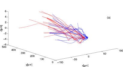
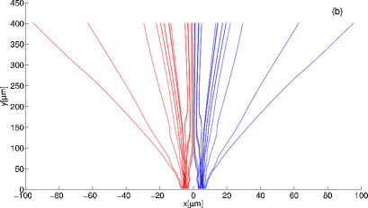
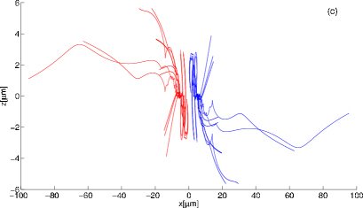
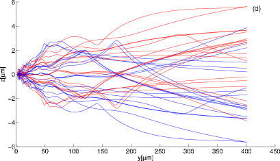
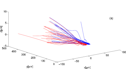
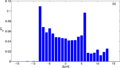
In Fig. 2, the photon trajectories associated with the diffraction of an incident EM field circularly polarized (, ) are plotted. The parameters considered in the simulation are: nm, m and m. The projections of these flow lines on the plane, shown in Fig. 2(b), are identical to those for incident linearly polarized light [45] (note that (72) is exactly the same as (71)). As shown elsewhere [54] within the context of Bohmian mechanics, for equations like (72), which describes the photon-trajectory projections on the , trajectories exiting through one slit never cross the trajectories coming up from the other one. Moreover, if both slits are identical (here this means they have the same width and transmission function), the EME fluxes coming out from each slit are symmetric with respect to the axis . Now, although neither the electric nor the magnetic field depend on the -coordinate, the photon trajectories display some remarkable features along this direction, as seen in Figs. 2(c) and 2(d). This is an effect of having circular (or elliptical, in general) polarization, which vanishes in the case of linear polarization, when or .
In order to understand the somewhat unexpected motion along the -direction, let us go back to (64). Rearranging terms and using (62) and (63), this equation can be rewritten as
| (74) |
where
| (75) |
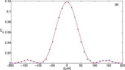
According to (74), the presence of a polarization state gives rise to a flow along the -direction in terms of the vorticity manifested by the fields and , which may lead the photon trajectories to display loops out of the plane. Nodal structures and other singularities and topological structures may then appear, as shown by Nye [55] within the context of wave dislocations [56] and by other authors within the context of the Riemann-Silberstein complex formulation of Maxwell’s equations [38, 57, 58] (see Appendix A). Experimentally, what one would observe on the plane is simply the typical fringe-like interference pattern constituted by dark and light parallel strips, which results from the accumulation of photons arriving at this plane. Note that (65) describes the interference pattern, which results from transporting the EME density through space (from the slits to some detection screen) in accordance to the guidance or continuity equation (10). This means that, if we make a histogram with the arrivals of a statistical distribution of photon trajectories along the -direction (from now on, we will label the normalized amount of such counts as , with ), the well-known interference pattern emerges, as can be seen in Fig. 3(a). However, from (75), all the arrivals at a certain height will not arise from positions at the slits at the same height , but there is a flux upwards and downwards which breaks the longitudinal (along the -direction) symmetry of the experiment when it is studied from the viewpoint of photon trajectories. This gives rise to a certain distribution of arrivals along the -direction, as shown in Fig. 3(b). Since the photon trajectories distribute evenly around (here, along positive and negative , since we have chosen ), as can be appreciated in Fig. 2(d), their distribution is also going to be symmetric with respect to in the histogram of Fig. 3(b). Nonetheless, we would like to point out that this effect along the -axis arises because we are considering a particular initial value of the -coordinate. If this coordinate is sampled properly up and down, this effect cannot be appreciated, but only a homogenous distribution, unlike what happens along the -coordinate.

6 The EM field and photon trajectories behind two slits, each followed by a linear polarizer
According to the Arago-Fresnel laws [46], if two diffracted beams with different polarization states interfere, the visibility of the interference pattern will decrease. Indeed, if the polarization states are orthogonal the pattern will disappear totally. In order to describe this effect with photon trajectories, we consider the EM field behind a grating with two slits, each followed by a linear polarizer, such that behind the slit 1 there is a polarizer with its polarization axis oriented along the -axis and behind the slit 2 the polarizer is oriented along the -axis. As in Sec. 4, we will also start expressing the total EM field in terms of the superposition of two fields, each propagating from one of the slits (see (60) and (61)). However, due to the presence of the polarizers and their filtering effect on the incident EM field, instead of Eqs. (25) and (26), now we will express the electric and magnetic fields in terms of and , described by (56), i.e.,
| (76) | |||
| (77) |
By substituting (76) and (77) into (23) and (24), we will obtain the EM field behind the two slits covered by the polarizers,
| (78) | |||||
| (79) |
From these fields, we obtain the expressions for the EME density and the Poynting vector,
| (80) | |||||
and
| (81) | |||||
| (82) | |||||
| (83) | |||||
respectively. As can be noticed in (80), describes the bare addition of EME densities associated with the fields diffracted by each slit, with no interference term. This means that no interference pattern is going to be observed at the detection screen, in accordance to the Arago-Fresnel law for the interference of two beams with orthogonal polarization states (perpendicularly polarized in the case of linear polarization [47] or with opposite handedness in the case of elliptic or circular polarization [48]). Regarding the Poynting vector, we note that the EME flux along the and -direction is also given by the simple addition of fluxes coming from each slit. Thus, unlike the diffraction problem dealt with in the previous section, now it is not possible to factorize the flux (neither the EME density) in terms of its spatial and polarization parts. This has a consequence on the EME flux along the -direction, which does not satisfy the rotational character described by (75). On the other hand, since the third and forth terms in (83) do not vanish, there will be an EME flux along the -direction even in the case of linear polarization (remember from Sec. 5 that, for linear polarization, ). This can also be seen from the photon-trajectory equations,
| (84) | |||||
| (85) |
Note in (84) that , effectively, does not vanish, not only for or (the conditions for linear polarization), but neither for any other value.

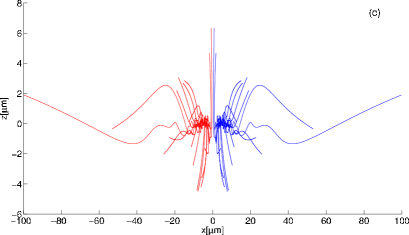

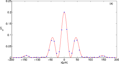
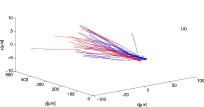
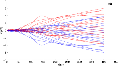
In Fig. 4, we observe an ensemble of photon trajectories for an incident EM field linearly polarized (, ). As before, the parameters considered in the simulation are: nm, m and m. As can be noticed, when polarizers with orthogonal polarization directions act on the diffracted wave, the topology of the flow lines changes dramatically when compared with that observed in Fig. 2. When one looks at the projection (see Fig. 4(b)), the wiggling behavior that gives rise to the different interference fringes of the pattern in the Fraunhofer region are lacking. This reflects the fact that the EME density, described by (80), is just the sum of the EME densities associated with the components of the wave that arise from each slit, which can be appreciated in the histogram presented in Fig. 5(a). This histogram reproduces the distribution pattern of the photon trajectories in the Fraunhofer region, which simply consists of the direct sum of the two single-slit diffraction patterns associated with the EM field arising from each slit. In particular, since the grating is assumed as fully transparent along the space covered by the slits and opaque elsewhere, the single-slit diffraction pattern is a square sinc function, this leading to the appearance of the maxima and minima observed in Fig. 5(a). The reason why this pattern looks like the one arising from a single slit rather than the sum of two of them is very simple. The observation distance (1 mm) is much larger than the distance between the two slits (10 m) and, therefore, the single-slit diffraction pattern associated with each slit basically overlap. For example, the first minima for slit 1 occur at m and m, while for slit 2 they are at m and m; therefore, the minima of the total pattern will appear at m, as can be seen in Fig. 5(a). It is worth mentioning that the loss of the interference fringes as well as the lack of wiggling features in the trajectories is similar to the behavior found in trajectories for massive particles in the case of decoherence [59, 60].
If we look at the topology of the photon trajectories along the -direction (see Figs. 4(c) and (d)), we note that there is a symmetry with respect to (see Fig. 4(c)). This is the result of the breaking of the rotationality property mentioned in the previous section. The same “symmetry” breaking can also be observed by looking at the distribution of the trajectories along the -direction, as shown in Fig. 5(b). If we changed the initial polarization state, from to , we would obtain the same pattern, but inverted with respect to . Again, as we discussed in Sec. 5, this is an effect arising from considering a particular initial value of the -coordinate for the photon trajectories, which will disappear when a sampling along the -axis is considered.


In the case of an incident EM field circularly polarized, displayed in Fig. 6, we find that the photon-trajectory projections on the plane (see Fig. 6(b)) look exactly the same as those for the incident EM field linearly polarized (see Fig. 4(b)), in accordance to Eq. (85). However, as seen in Sec. 5, due to the rotationality associated with circular polarization, a breaking of the specular symmetry with respect to will take place, and the EME flux leaving each slit is going to be different, as shown in Figs. 6(c) and 6(d). This will give rise to a histogram like the one shown in Fig. 5(a) when photon are counted along the -direction and another similar to that of Fig. 3(b) when they are counted along the -direction.
7 Final discussion and conclusions
Interference experiments with non-relativistic massive particles and photons can be well understood on the theoretical grounds provided by the (non-relativistic) Schrödinger and Maxwell equations, respectively. Thus, if one wishes to determine photon trajectories on the same footing as Bohmian trajectories, the most appropriate theoretical framework is the one based on Maxwell’s equations, more specifically their hydrodynamical formulation, proposed by Bialynicki-Birula [27, 28, 29, 30]. Within this formulation, a close analogy can be established between the trajectory equations based on the latter and Bohm’s approach when the particle aspect of both light and matter is taken into consideration. This allows to compare on the same grounds the (Bohmian) trajectories for massive particles with the trajectories derived for photons from classical electromagnetism. The photon trajectories (EME flow lines) are determined from the Poynting vector, with the components of the electric and magnetic vector fields expressed in terms of a function that explicitly takes into account the boundary conditions imposed by the grating. It is remarkable that, in the case of photons, any trajectory-based interpretation will be complementary to the standard Huyghens’ one, based on the superposition of secondary wavelets. Furthermore, the topology displayed by the photon trajectories is strikingly similar to that displayed by massive particles. As happens in the case of massive particles [14], such a topology can also be inferred and explained from the corresponding trajectory equation.
Here, we have considered the Bialynicki-Birula hydrodynamical framework to analyze the effects of polarization on interference pattern for waves which arise from an initially polarized monochromatic EM plane wave. According to the Arago-Fresnel laws of interference with polarized light in Young-type experiments [46], if, for example, the two interfering beams are linearly polarized in orthogonal directions [47] or both are elliptically polarized but with opposite handedness [48], no interference will be observed. The photon trajectories presented in this work show how the EME density distributes in configuration space, giving rise to the appearance or not of interference fringes. This thus constitutes a very interesting corpuscular-like description of the Arago-Fresnel laws for the interference of polarized light, consistent with the more standard wave description. Moreover, it is clear that the photon wave function can be interpreted as an energy localization amplitude or detection amplitude within the hydrodynamical approach to Electromagnetism. Now, from the agreement between the histograms and the corresponding EME density distribution (which follows from (10) or (11)), this density can also be understood as a probability density function in the sense that arrivals are going to distribute statistically according to it, as can be seen in the recent experiment carried out by Dimitrova and Weis [4], for example.
Acknowledgements
MD and MB acknowledge support from the Ministry of Science of Serbia under Project “Quantum and Optical Interferometry”, No. 141003; ASS and SMA acknowledge support from the Ministerio de Ciencia e Innovación (Spain) under Project FIS2007-62006. ASS also thanks the Consejo Superior de Investigaciones Científicas (Spain) for a JAE-Doc Contract.
Appendix A Appendix A: Photon trajectories within the Riemann-Silberstein formulation of Electromagnetism
Both Maxwell’s and Schrödinger’s equations describe the evolution of fields in configuration space, namely the EM field and probability fields associated with non-relativistic massive particles, respectively. From these fields, one can obtain trajectories which show how they evolve in space, namely photon trajectories or Bohmian trajectories, respectively. However, Maxwell’s equations look quite different formally from the Schrödinger equation as they are usually given. A formulation that allows one to put Maxwell’s equations on similar formal grounds as Schrödinger’s one (but without due to the lack of mass of photons) is the complex form of Maxwell’s equations [43, 44], which is based on the so-called Riemann-Silberstein complex EM vector [27, 28],
| (86) |
with the change of variable
| (87) | |||||
| (88) |
where and are real fields. Introducing (87) and (88) into Maxwell’s equations in the absence of electrical charge densities, we obtain
| (89) | |||||
| (90) |
As can be noticed, (89) is the analog for photons of the Dirac equation for massive particles, while (90) describes the conservation of the EME density through space. This analogy within the Riemann-Silberstein formulation becomes more apparent by gathering (89) and (90) in a single equation. This is done by applying the operator to both sides of (89) and then rearranging terms taking into account (90) and the vectorial relation
| (91) |
where is a general vector field. This renders
| (92) |
which has the well-known form of the Klein-Gordon equation. In the particular case of diffraction problems, which can be reduced to boundary condition problems because of their time-independence, the space and time parts of (92) are separable. Thus, can be decomposed as
| (93) |
where the space part, , satisfies Helmholtz’s equation,
| (94) |
and its time-dependent part the differential equation
| (95) |
with .
Within this formulation, the EME density is given by
| (96) |
and its flux, described by the Poynting vector, is straightforwardly obtained after developing the time-derivative of to yield
| (97) |
where the relation
| (98) |
for any two vectors, and , has been taken into account. From these magnitudes, we can now obtain the stationary photon trajectories within the Riemann-Silberstein formulation as,
| (99) |
(here, denotes the time-average of the magnitude ), which transport the time-averaged EME density, , as described by the (also time-averaged) Poynting vector, .
If the electric and magnetic fields are complex and the definition of the Riemann-Silberstein vector is kept as in (86), i.e., the real and imaginary parts are given by the electric and magnetic fields, respectively, then we need to include into the formulation two of these vectors in order to have a complete description of the problem, each one associated with the real or the imaginary parts of the electric and magnetic fields. That is, if
| (100) |
with and () being real vector fields satisfying the corresponding Maxwell equations, we will have
| (101) |
The EME density (96) and the Poynting vector (97) then read as
| (102) | |||||
| (103) |
respectively, and their time-averaged homologous, assuming the decomposition (93), as
| (104) | |||||
| (105) |
References
- [1] A. Tonomura, J. Endo, T. Matsuda, T. Kawasaki, H. Ezawa, Am. J. Phys. 57 (1989) 117.
- [2] F. Shimizu, K. Shimizu, H. Takuma, Phys. Rev. A 46 (1992) R17.
- [3] S. Parker, Am. J. Phys. 39 (1971) 420; 49 (1972) 1003.
- [4] T.L. Dimitrova, A. Weis, Am. J. Phys. 76 (2008) 137.
- [5] http://ophelia.princeton.edu/page/single-photon.html
- [6] M. Born, Z. Phys. 37 (1926) 863 (1926); 38 (1926) 803; Nature 119 (1927) 354.
- [7] R. Loudon, The Quantum Theory of Light, Oxford University Press, Oxford, 1983.
- [8] C. Philippidis, C. Dewdney, B.J. Hiley, Nuovo Cimento B52 (1979) 15.
- [9] A.S. Sanz, F. Borondo, S. Miret-Artés, Phys. Rev. B 61 (2000) 7743.
- [10] A.S. Sanz, F. Borondo, S. Miret-Artés, J. Phys.: Condens. Matter 14 (2002) 6109.
- [11] R. Guantes, A.S. Sanz, J. Margalef-Roig, S. Miret-Artés, Surf. Sci. Rep. 53 (2004) 199.
- [12] A.S. Sanz, S. Miret-Artés, in: D. Micha, I. Burghardt (Eds.), Quantum Dynamics of Complex Molecular Systems, Vol. 83, Springer, New York, 2006, p. 343.
- [13] M. Gondran, A. Gondran, Am. J. Phys. 73 (2005) 507.
- [14] A.S. Sanz, S. Miret-Artés, J. Chem. Phys. 126 (2007) 234106.
- [15] M. Davidović, D. Arsenović, M. Božić, A.S. Sanz, S. Miret-Artés, Eur. Phys. J.-Spec. Top. 160 (2008) 95.
- [16] M. Božić, D. Arsenović, Acta Phys. Hung. B 26 (2006) 219.
- [17] E. Madelung, Z. Phys. 40 (1926) 322.
- [18] D. Bohm, Phys. Rev. 85 (1952) 166; 85 (1952) 184.
- [19] T. Takabayashi, Prog. Theor. Phys. 8 (1952) 143; 9 (1953) 187.
- [20] P.R. Holland, The Quantum Theory of Motion, Cambridge University Press, Cambridge, 1993.
- [21] D. Dürr, S. Teufel, Bohmian Mechanics, Springer, Berlin, 2009.
- [22] W. Braunbek, G. Laukien, Optik 9 (1952) 174.
- [23] R.D. Prosser, Int. J. Theor. Phys. 15 (1976) 169.
- [24] R.D. Prosser, Int. J. Theor. Phys. 15 (1976) 181.
- [25] J.D. Jackson, Classical Electrodynamics, Wiley, New York, 1998, 3rd ed.
- [26] P. Ghose, A.S. Majumdar, S. Guha, J. Sau, Phys. Lett. A 290 (2001) 205.
- [27] I. Bialynicki-Birula, Acta Phys. Pol. 86 (1994) 97.
- [28] I. Bialynicki-Birula, in: J.H. Eberly, L. Mandel, E. Wolf (Eds.), Coherence and Quantum Optics, Vol. 8, Plenum, New York, 1996, p. 313.
- [29] I. Bialynicki-Birula, Prog. Opt. 36 (1996) 245.
- [30] I. Bialynicki-Birula, in: E. Infeld, R. Zelazny, A. Galkowski (Eds.), Nonlinear Dynamics, Chaotic and Complex Systems, Cambridge University Press, Cambridge, 1997, p. 64.
- [31] J.E. Sipe, Phys. Rev. A 52 (1995) 1875.
- [32] L.D. Landau, R. Peierls, Z. Phys. 62 (1930) 188.
- [33] P.A.M. Dirac, The Principles of Quantum Mechanics, Clarendon Press, Oxford, 1958.
- [34] R.J. Cook, Phys. Rev. A 25 (1982) 2164; 26 (1982) 2754.
- [35] T. Inagaki, Phys. Rev. A 49 (1994) 2839.
- [36] M.O. Scully, M.S. Zubairy, Quantum Optics, Cambridge University Press, Cambridge, 1997.
- [37] D.H. Kobe, Found. Phys. 29 (1999) 1203.
- [38] M.V. Berry, J. Opt. A 6 (2004) S175.
- [39] P.R. Holland, Proc. R. Soc. A 461 (2005) 3659.
- [40] M.G. Raymer, B.J. Smith, Proc. SPIE 5866 (2005) 1.
- [41] B.J. Smith, M.G. Raymer, New J. Phys. 9 (2007) 414.
- [42] W. Zhi-Yong, X. Cai-Dong, K. Ole, Chin. Phys. Lett. 24 (2007) 418.
- [43] L. Silberstein, Ann. Phys. 22 (1907) 579; 24 (1907) 783.
- [44] H. Bateman, The Mathematical Analysis of Electrical and Optical Wave Motion on the Basis of Maxwell’s Equations, Dover, New York, 1955.
- [45] M. Davidović, A.S. Sanz, D. Arsenović, M. Božić, S. Miret-Artés, Phys. Scr. T135 (2009) 14009.
- [46] R. Barakat, J. Opt. Soc. Am. A 10 (1993) 180.
- [47] J.L. Hunt, G. Karl, Am. J. Phys. 38 (1970) 1249.
- [48] D. Pescetti, Am. J. Phys. 40 (1972) 735.
- [49] M. Born, E. Wolf, Principles of Optics, Pergamon Press, Oxford, 2002, 7th ed.
- [50] M. Božić, D. Arsenović, L. Vušković, Z. Naturf. A56 (2001) 173.
- [51] D. Arsenović, M. Božić, O.V. Man’ko, V.I. Man’ko, J. Russ. Laser Res. 26 (2005) 94.
- [52] M. Davidović, M. Božić, D. Arsenović, J. Russ. Laser Res. 27 (2006) 220.
- [53] D. Arsenović, M. Božić, L. Vušković, J. Opt. B: Quantum Semiclass. Opt. 4 (2002) S358.
- [54] A.S. Sanz, S. Miret-Artés, J. Phys. A 41 (2008) 435303.
- [55] J.F. Nye, Proc. R. Soc. Lond. A 387 (1983) 105; 389 (1983) 279.
- [56] J.F. Nye, M.V. Berry, Proc. R. Soc. Lond. A 336 (1974) 165.
- [57] I. Bialynicki-Birula, Z. Bialynicka-Birula, Phys. Rev. A 67 (2003) 062114.
- [58] G. Kaiser, J. Opt. A: Pure Appl. Opt. 6 (2003) S243.
- [59] A.S. Sanz, F. Borondo, Eur. Phys. J. D 44 (2007) 319.
- [60] A.S. Sanz, F. Borondo, Chem. Phys. Lett. 478 (2009) 301.
- [61] A.G. Borisov, S.V. Shabanov, J. Comp. Phys. 209 (2005) 643; 216 (2006) 391.
- [62] A.G. Borisov, F.J. García de Abajo, S.V. Shabanov, Phys. Rev. B 71 (2005) 075408.