Multigrid and preconditioning strategies for implicit PDE solvers for degenerate parabolic equations

Abstract

The novel contribution of this paper relies in the proposal of a fully implicit numerical method designed for nonlinear degenerate parabolic equations, in its convergence/stability analysis, and in the study of the related computational cost. In fact, due to the nonlinear nature of the underlying mathematical model, the use of a fixed point scheme is required and every step implies the solution of large, locally structured, linear systems. A special effort is devoted to the spectral analysis of the relevant matrices and to the design of appropriate iterative or multi-iterative solvers, with special attention to preconditioned Krylov methods and to multigrid procedures: in particular we investigate the mutual benefit of combining in various ways suitable preconditioners with V-cycle algorithms. Numerical experiments in one and two spatial dimensions for the validation of our multi-facet analysis complement this contribution. AMS SC: 65N12, 65F10 (65N22, 15A18, 47B35)

1 Introduction

We consider a single equation of the form

$$\frac{\partial u}{\partial t}=\nabla\cdot\left(D(u)\nabla u\right),$$ (1)

where $D(u)$ is a non-negative function. The the equation is parabolic and it called degenerate whenever $D(u)$ vanishes for some values of $u$. For the convergence analysis of our numerical methods, we will require that $D(u)$ is at least differentiable and that $D^{\prime}(u)$ is Lipschitz continuous, while the existence of solutions is guaranteed under the milder assumption of continuity (see Vázquez, 2007).

The classical porous medium equation (where $D(u)$ is restricted to be a power law) or its generalized form have important applications in many fields of science. Their name arise from the model of Darcy’s flow of a gas through a porous medium ($D(u)=\kappa u^{\gamma}$ where $\gamma$ is the specific heat ratio), but classical applications range from ground-water flow (Boussinesq equation) to spatial population dynamics (where crowding effects require nonlinear degenerate diffusion terms). Moreover models based on equation (1) have been proposed as useful approximations of more complex models like thin films motion (when disregarding surface tension), water-oil mixtures in porous medium, boundary layer in fluid flow past an obstacle, magma in volcanoes, etc. More recently they have been studied as limits of kinetic particle models, with applications for the diffusion in semiconductors. Finally we mention that some contrast-enhancement filters for image processing like the one by Perona-Malik are based on (1). For more details on the aplications, see e.g. Vázquez (2007, Chap 2 and 21) and the references therein.

The present investigation is part of the search for suitable numerical techniques to integrate for long times nonlinear, possibly degenerate, parabolic equations appearing in models for monument degradation (see Aregba Driollet et al. (2004)) when chemical/micro-biological pollutants are taken into consideration. We wish to point out that the techniques developed here have applications that go beyond the aforementioned models. For example, again in the area of conservation of the cultural heritage, they could be adapted to numerically investigate the more complete sulfation model described in Alì et al. (2007) and the consolidation model presented in Clarelli et al. (2009). Some applications in the field of monument conservation have been presented in Semplice et al. (2009), where the mathematical tools developed in the present paper are employed for forecasting marble deterioration. Of course, in such a context, given the wide variety of artefacts, an important challenge is the combination of the approximation scheme with the related linear algebra solvers, in presence of complicate geometries and griddings.

In the literature, degenerate parabolic equations have been discretized mainly using explicit or semi-implicit methods, thus avoiding to solve the nonlinear equation arising from the elliptic operator. A remarkable class of methods arise directly from the so-called non-linear Chernoff formula Brézis & Pazy (1972) for time advancement, coupling it with a spatial discretization: for finite differences the latter study was started in Berger et al. (1979) and for finite elements in Magenes et al. (1987). More recently, another class related to the relaxation approximation emerged: such numerical procedures exploit high order non-oscillatory methods typical of the discretization of conservation laws and their convergence can be proved making use of semigroup arguments similar to those relevant for proving the Chernoff formula (Cavalli et al., 2007).

In this paper we start from the Crandall-Liggett formula

$$U(t^{n},x)-\mathrm{\Delta}tL_{D}(U(t^{n},x))=U(t^{n-1},x),$$ (2)

where time has been discretized with steps $\mathrm{\Delta}t=t^{n}-t^{n-1}$, and $-L_{D}(\cdot)$ denotes the elliptic operator $u\mapsto-\nabla\cdot(D(u)\nabla u)$. The computation of the numerical solution $U(t^{n},x)$ requires to solve a nonlinear equation whose form is determined by the elliptic operator and the nonlinear function $D(u)$, but the convergence is guaranteed without restrictions on the time step $\mathrm{\Delta}t$ (Crandall & Liggett, 1971). Furthermore, due to the nonlinear nature of the underlying mathematical model, the use of a fixed point scheme is required and the choice of the Newton-like methods implies the solution at every step of large, locally structured (in the sense of Tilli, 1998) linear systems. A special effort is devoted to the spectral analysis of the relevant matrices and to the design of appropriate iterative or multi-iterative solvers (see Serra-Capizzano, 1993), with special attention to preconditioned Krylov methods and to multigrid procedures (see Greenbaum (1997); Saad (2003); Hackbusch (1985); Trottenberg et al. (2001) and references therein for a general treatment of iterative solvers). Although most of the analysis is developed in the one-dimensional case (from Section 2 to Section 4), we also indicate in Section 5 how to generalize our approach to two spatial dimensions. we also perform numerical experiments for the validation of our analysis in both settings (see Section 4 and Section 5, respectively).

The paper is organized as follows. In Section 2 we couple the time discretization (2) with a spatial discretization based on finite differences and set up a Newton method for the resulting system of nonlinear equations. We report the explicit form of the Jacobian appearing in the Newton iterations and we prove the convergence of the Newton methods under a mild restriction on $\mathrm{\Delta}t$. In Section 3 we consider various iterative methods for the solution of the inner linear systems involved in the Newton method. A brief spectral analysis of the related matrix structures is provided in order to give an appropriate motivation for the good behaviour of the proposed iterative and multi-iterative solvers. In Section 4 we perform some numerical tests. In Section 5 we describe a generalization of the previous methods to a two-dimensional case and perform numerical tests in this setting too. Finally, a conclusion section with a short plan for future investigations completes the paper.

2 Numerical methods in one dimension

In order to discretize equations like (1), we will employ a time semi-discretization given by the Crandall-Liggett formula and a space discretization based on finite differences, explained in the following subsection. The latter numerical choice leads to a system of coupled nonlinear equations that need to be solved at each discrete timestep in order to compute the solution of the PDE: this is achieved using the Newton method, as detailed in Subsection 2.2, where we also prove and comment convergence results.

2.1 Finite difference discretization

We take into consideration a standard discretization in space using finite differences. Denoting $x_{\xi}=a+\xi h$, we consider $N+2$ points with equal spacing $h=(b-a)/(N+1)$ in the interval $[a,b]$ and we denote by $u^{n}_{k}$ the approximate solution at time $t^{n}$ and location $x_{k}$, where $k=0,\ldots,N+1$. Let $\mathbf{u}^{n}$ be the vector containing the collection of the unknown values $u^{n}_{k}$. When no potential confusion can arise, we will sometimes drop in both notations the superscript indicating the time level. Of course, when considering Dirichlet boundary conditions, the values $u_{0}$ and $u_{N+1}$ are known and can be eliminated by the equations, leaving a vector of unknowns $\mathbf{u}^{n}$ that contains only $u_{k}^{n}$ for $k=1,\ldots,N$. Boundary conditions of Neumann or Robin type can be treated in similar ways.

We choose a standard 3-points second order approximation of the differential operator $(D(u)u_{x})_{x}$. Denoting with the subscript $\xi$ the evaluation at the point $x_{\xi}$, we have that:

$$\left.\frac{\partial}{\partial x}\left(D(u)\tfrac{\partial u}{\partial x}\right)\right|_{j}=\frac{D(u)_{j+1/2}\left.\tfrac{\partial u}{\partial x}\right|_{j+1/2}-D(u)_{j-1/2}\left.\tfrac{\partial u}{\partial x}\right|_{j-1/2}}{h}+o(1)\\ =\frac{D(u)_{j+1/2}(u_{j+1}-u_{j})-D(u)_{j-1/2}(u_{j}-u_{j-1})}{h^{2}}+o(1)\\ =\frac{(D(u_{j+1})+D(u_{j}))(u_{j+1}-u_{j})-(D(u_{j})+D(u_{j-1}))(u_{j}-u_{j-1})}{2h^{2}}+o(1)$$ (3)

where the $o(1)$ error term is of order $h^{2}$ under the assumption that the composition

$$\phi(\cdot)=D(u(\cdot))$$

is at least continuously differentiable, with Lipschitz continuous first derivative. Putting together all the contributions for different grid points, we end up with $L_{D(\mathbf{u})}\mathbf{u}$, where the tridiagonal matrix

$$L_{D(\mathbf{u})}=\begin{bmatrix}-D_{1/2}-D_{3/2}&D_{3/2}&\\ D_{3/2}&-D_{3/2}-D_{5/2}&D_{5/2}&\\ &D_{5/2}&\ddots&\ddots&\\ &&\ddots&\ddots&D_{N-1/2}\\ &&&D_{N-1/2}&-D_{N-1/2}-D_{N+1/2}\\ \end{bmatrix}$$ (4)

conatins the values

$$D_{j+1/2}=\frac{D(u_{j+1})+D(u_{j})}{2}\,,\qquad j=0,\ldots,N,$$

and thus depends nonlinearly on the $u_{j}$’s. It should be noticed that the latter is a second order approximation of $\phi(x_{j+1/2})$ since $u^{n}_{k}$ differs from $u(t^{n},x_{k})$ by $O(h^{2})$ thanks to the second order scheme and since, by standard Taylor expansions, we have

$$D_{j+1/2}=\frac{D(u_{j+1})+D(u_{j})}{2} = \frac{\phi(x_{j+1})+\phi(x_{j})}{2}+O(h^{2})$$

$$= \phi(x_{j+1/2})+\frac{h^{2}}{8}\phi_{xx}(\eta(h,j))+O(h^{2})$$

$$= \phi(x_{j+1/2})+O(h^{2}),\ \quad\eta(h,j)\in(x_{j-1},x_{j}),$$

under the mild assumption that $\phi_{xx}(\cdot)$ is a bounded function. Of course, the same conclusion holds if $\phi_{x}(\cdot)$ is Lipschitz continuous.

In the following, we denote by $\mathsf{tridiag}_{k}[\beta_{k},\alpha_{k},\gamma_{k}]$ a square tridiagonal matrix of order $N$ with entries $\beta_{k}$ on the lower diagonal, $k=2,\cdots,N$, $\alpha_{k}$ on the main diagonal, $k=1,\cdots,N$, and $\gamma_{k}$ on the upper diagonal, $k=1,\cdots,N-1$. With this notation, $L_{D(\mathbf{u})}=\mathsf{tridiag}_{k}[D_{k-1/2},-D_{k-1/2}-D_{k+1/2},D_{k+1/2}]$. We also denote with $\mathsf{diag}_{k}[\alpha_{k}]$ the square diagonal matrix with $\alpha_{k}$ on the $k^{\text{th}}$ row.

As already observed $L_{D(\mathbf{u})}$ is a symmetric real tridiagonal matrix. Since $D(\cdot)$ is a nonnegative function, the matrix $-L_{D(\mathbf{u})}$ is always positive semidefinite, beacuse it is weakly diagonally dominant by row, or equivalently thanks to the first Gerschgorin Theorem (see e.g. Golub & Van Loan, 1996). Furthermore, we have positive definiteness (i.e. invertibility), at least for every $N$ large enough, if in addition $\phi(\cdot)$ has only isolated zeros in $(a,b)$. In that case, for $N$ large enough, the matrix is irreducible or block diagonal with irreducible blocks. In particular, when $\phi(\cdot)$ is strictly positive in $(a,b)$ then $-L_{D(\mathbf{u})}$ is positive definite and irreducible for any $N$.

When introducing numerical methods for the approximation of the differential equation we will encounter nonlinear systems involving the matrices $-L_{D(\mathbf{u})}$. At that point more sophisticated (spectral) relations and features will be discussed, when choosing the appropriate iterative solvers for the global linearised system (see Subsection 3.1). For the moment we just observe that, thanks to the previous preliminary spectral analysis, all the classical iterative solvers like Jacobi and Gauss-Seidel (and their damped version with damping parameter belonging to $(0,2)$) are all convergent for the solution of a linear system with such a coefficient matrix. The problem is that the spectral radii are very close to $1$, with a gap ranging between $O(N^{-2})$, reached by all these classical iterations with the only exception of the optimally damped Gauss-Seidel, and $O(N^{-1})$, reached for Gauss-Seidel with optimal damping parameter (see Varga, 1962). When considering the whole system things become slightly better since the gap between the spectral radius and $1$ reduces for all the considered procedures to $O(N^{-1})$. However, as a partial conclusion, we can safely claim the considered iterations would be unacceptably slow and the search for specialised iterative solvers becomes mandatory. This latter is the main subject of Section 3.

2.2 The nonlinear system and the Newton iteration

Following the Crandall-Liggett formula (2), in order to compute $\mathbf{u}^{n}$ from $\mathbf{u}^{n-1}$, we need to solve the nonlinear vector equation

$$\mathbf{u}^{n}=\mathbf{u}^{n-1}+\frac{\mathrm{\Delta}t}{h^{2}}L_{D(\mathbf{u}^{n})}\mathbf{u}^{n}$$

and thus we set up Newton iterations for the vector function

$$F(\mathbf{u})=\mathbf{u}-\frac{\mathrm{\Delta}t}{h^{2}}L_{D(\mathbf{u})}\mathbf{u}-\mathbf{u}^{n-1}.$$ (5)

In the following, we denote $\mathbf{u}^{n,s}$ the $s^{\text{th}}$ Newton iterate for the computation of $\mathbf{u}^{n}$. The generic partial derivative of $F(\mathbf{u})$ is

$$\frac{\partial F_{k}}{\partial u_{j}}=\delta_{jk}-\frac{\mathrm{\Delta}t}{h^{2}}\left.L_{D(\mathbf{u})}\right|_{j,k}-\frac{\mathrm{\Delta}t}{2h^{2}}\left[\begin{aligned} &\delta_{k-1,j}D^{\prime}_{k-1}(u_{k-1}-u_{k})+\\ &+\delta_{k,j}D^{\prime}_{k}(u_{k-1}-2u_{k}+u_{k+1})+\\ &+\delta_{k+1,j}D^{\prime}_{k+1}(u_{k+1}-u_{k}).\end{aligned}\right]\,,$$ (6)

so that the Jacobian is

$$F^{\prime}(\mathbf{u}) =X_{N}(\mathbf{u})+Y_{N}(\mathbf{u}),$$ (7)

$$X_{N}(\mathbf{u}) =I_{N}-\frac{\mathrm{\Delta}t}{h^{2}}L_{D(\mathbf{u})},$$ (8)

$$Y_{N}(\mathbf{u}) =-\frac{\mathrm{\Delta}t}{2h^{2}}T_{N}(\mathbf{u})\mathsf{diag}_{k}[D^{\prime}_{k}],$$ (9)

$$T_{N}(\mathbf{u}) =\mathsf{tridiag}_{k}[u_{k-1}-u_{k},u_{k-1}-2u_{k}+u_{k+1},u_{k+1}-u_{k}].$$ (10)

The matrix $X_{N}(\mathbf{u})$ is symmetric positive definite and $\lambda_{\text{min}}(X_{N}(\mathbf{u}))\geq 1$, where $\lambda_{\text{min}}(A)$ denotes the minimum eigenvalue of the matrix $A$. We note that the inequality is strict under assumption of isolated zeros. If $\mathsf{diag}_{k}[D^{\prime}_{k}]$ is positive semidefinite, i.e. if $D(\cdot)$ is a smooth nondecreasing function, then, setting $E^{2}=\mathsf{diag}_{k}[D^{\prime}_{k}]$, $E$ is a positive semidefinite diagonal matrix and $Y_{N}(\mathbf{u})$ is similar to $-\frac{\mathrm{\Delta}t}{2h^{2}}ET_{N}(\mathbf{u})E$. Moreover, defining

$$\tilde{Y}_{N}(\mathbf{u}) =-\frac{\mathrm{\Delta}t}{2h^{2}}\tilde{T}_{N}(\mathbf{u})\mathsf{diag}_{k}[D^{\prime}_{k}],$$ (11)

$$\tilde{T}_{N}(\mathbf{u}) =\mathsf{tridiag}_{k}[u_{k-1}-u_{k},0,u_{k+1}-u_{k}]=T_{N}(\mathbf{u})-\mathsf{diag}_{k}[u_{k-1}-2u_{k}+u_{k+1}],$$ (12)

we have that $\tilde{Y}_{N}(\mathbf{u})$ is similar to $-\frac{\mathrm{\Delta}t}{2h^{2}}E\tilde{T}_{N}(\mathbf{u})E$, with the latter being anti-symmetric, which implies a pure imaginary spectrum.

In the following we will denote by $\|\cdot\|$ the Euclidean norm for vectors and the induced spectral norm for matrices.

Remark 2.1.

If $\mathbf{u}$ is a sampling of a solution $u$ of (1) at least continuous and $\omega_{u}(\cdot)$ denotes its modulus of continuity, then

$$\|Y_{N}(\mathbf{u})\|\leq e_{u}(\mathrm{\Delta}t,h)$$

with

$$e_{u}(\mathrm{\Delta}t,h)=4\frac{\mathrm{\Delta}t}{h^{2}}\|D^{\prime}(u)\|_{\infty}\omega_{u}(h).$$

In order to deduce the latter, it is enough to recall that for normal matrices the spectral norm is bounded by any induced norm and in particular by the the matrix norm induced by the infinity vector norm. In particular, if $u$ is Hölder continuous with exponent $\alpha\in(0,1]$ and constant $M>0$, then the estimate above can be written as

$$e_{u}(\mathrm{\Delta}t,h)=4M\frac{\mathrm{\Delta}t}{h^{2-\alpha}}\|D^{\prime}(u)\|_{\infty}.$$

Of course if $u$ is continuously differentiable, then we find $\alpha=1$ and $M=\|u^{\prime}\|_{\infty}$. Furthermore, when $u$ is two times continuously differentiable, we notice that $u_{k-1}-2u_{k}+u_{k+1}=h^{2}u^{\prime\prime}(\xi_{k})$ which leads to a more refined expression i.e.

$$e_{u}(\mathrm{\Delta}t,h)=\left(2\frac{\mathrm{\Delta}t}{h}\|u^{\prime}\|_{\infty}+\mathrm{\Delta}t\|u^{\prime\prime}\|_{\infty}\right)\|D^{\prime}(u)\|_{\infty}.$$

Finally, if we are interested in evaluating $\|Y_{N}(\mathbf{\tilde{u}})\|$ where $\tilde{u}$ is an approximation to the true solution $u$ (this happens naturally in the numerical process discussed in the present section), then

$$\|Y_{N}(\mathbf{\tilde{u}})\|\leq e_{\tilde{u}}(\mathrm{\Delta}t,h)\leq e_{u}(\mathrm{\Delta}t,h)+4\frac{\mathrm{\Delta}t}{h^{2}}\|D^{\prime}(u)\|_{\infty}\|u-\tilde{u}\|_{\infty}=4\frac{\mathrm{\Delta}t}{h^{2}}\|D^{\prime}(u)\|_{\infty}\left(\omega_{u}(h)+\|u-\tilde{u}\|_{\infty}\right).$$

Hence, since we are using second order formulae, the error $\|u-\tilde{u}\|_{\infty}=O(h^{2})$ and therefore $\|Y_{N}(\mathbf{\tilde{u}})\|$ is dominated by $\omega_{u}(h)$, which is of order $h$ if the solution is Lipschitz continuous, that is

$$\|Y_{N}(\mathbf{\tilde{u}})\|\leq 4M\frac{\mathrm{\Delta}t}{h}\|D^{\prime}(u)\|_{\infty}+O(\mathrm{\Delta}t).$$

In conclusion, we can safely claim that the global spectrum of the Jacobian $F^{\prime}(\mathbf{\tilde{u}})$ is decided, up to small perturbations, by the matrix $X_{N}(\mathbf{\tilde{u}})$. For making more explicit the latter statement, if we assume that $\mathrm{\Delta}t=Ch$, where $C>0$ is independent of $h$, then $\lambda_{\text{min}}(X_{N}(\mathbf{u}))\geq 1$, $\|X_{N}(\mathbf{\tilde{u}})\|=O(h^{-1})$, while $\|Y_{N}(\mathbf{\tilde{u}})\|=O(1)$.

In order to prove the convergence of the Newton method, we first consider some auxiliary results.

Lemma 2.1.

For a generic matrix $A$, the minimum singular value is

$$\sigma_{\rm min}(A)\geq\lambda_{\rm min}\left(\frac{A+A^{\mathsf{T}}}{2}\right).$$ (13)

Proof.

Consider the symmetric matrix

$$B=\left[\begin{aligned} &0&A^{\mathsf{T}}\\ &A&0\end{aligned}\right]$$

with eigenvalues $\lambda_{1}(B)=\sigma_{1}(A)\geq\dots\geq\lambda_{N}(B)=\sigma_{N}(A)\ \geq\lambda_{N+1}(B)=-\sigma_{N}(A)\geq\dots\geq\lambda_{2N}(B)=-\sigma_{1}(A)$, since the Schur decomposition of $B$ is easily written in terms of the singular value decomposition of $A$ (see Bhatia, 1997; Golub & Van Loan, 1996). Let $\cal V$ be a vector space and $\mathbf{x}\in\mathbb{R}^{N}$ such that $\|\mathbf{x}\|_{2}>0$. Thanks to the minimax principle (Bhatia, 1997), we obtain

$$\sigma_{\rm min}(A)=\lambda_{N}(B)=\max_{\dim({\cal V})=N}\;\min_{\mathbf{y}\in{\cal V}}\frac{\mathbf{y}^{T}B\mathbf{y}}{\mathbf{y}^{T}\mathbf{y}}\geq\min_{\begin{subarray}{c}\mathbf{y}=[\mathbf{x}^{T}\!\!,\;\mathbf{x}^{T}]^{T}\\ \mathbf{x}\in\mathbb{R}^{N}\end{subarray}}\frac{\mathbf{y}^{T}B\mathbf{y}}{\mathbf{y}^{T}\mathbf{y}}=\min_{\mathbf{x}\in\mathbb{R}^{N}}\frac{\mathbf{x}^{T}(A^{T}+A)\mathbf{x}}{2\mathbf{x}^{T}\mathbf{x}}=\lambda_{\rm min}\left(\frac{A+A^{T}}{2}\right).$$

∎

Remark 2.2.

The proof technique used for bounding from below the minimal singular value of a matrix $A$ is part of a more general framework useful for refining, when necessary, the estimates. In fact, in general it can be proved that for any complex-valued matrix $A$ the minimal singular value is not less than the distance $d_{r}$ of any straight line $r$ separating the numerical range of $A$ from the complex zero. Therefore a better estimate can be obtained by computing the sup (that we call $d$) of $d_{r}$, over all straight lines that induce the separation. In our case we used the fact that the real part of $A$ (that is ${\rm Re}(A)=(A+A^{\mathsf{T}})/2$) is positive definite and so our straight line becomes the set of all complex numbers having real part equal to $\lambda_{\rm min}({\rm Re}(A))$. The estimate could be poor since the latter straight line is not necessarily tangent to the numerical range (a convex set by the Toeplitz-Hausdorff theorem, see Bhatia (1997)): thus $d$ could be much larger than $d_{r}$. However in our setting such an estimate is already very satisfactory, as also stressed by the numerical experiments.

Proposition 2.3.

Consider $F(\mathbf{u})$ as defined in (5), where $\mathbf{u}$ is a sampling (at a given time $t$) of a solution $u$ of (1) with $D$ differentiable and having first derivative Lipschitz continuous. If, in addition, $\mathbf{u}$ is differentiable with Lipschitz continuous first derivative, then

$$\left\|F^{\prime}(\mathbf{u})^{-1}\right\|\leq 1+O(\mathrm{\Delta}t).$$ (14)

When using the induced $l^{\infty}$ norm, we have

$$\left\|F^{\prime}(\mathbf{u})^{-1}\right\|_{\infty}\leq C_{1}$$ (15)

for $h$ sufficiently small and under the additional assumption that $\mathrm{\Delta}t\leq C_{\infty}h$ for some $C_{\infty}>0$.

Proof.

For the sake of notational simplicity, we set $A=F^{\prime}(\mathbf{u})$. First of all we write the symmetric part of $A$ as

$$\frac{A+A^{\mathsf{T}}}{2}=X_{N}(\mathbf{u})+Z_{N}(\mathbf{u})\,,$$

where

$$Z_{N}(\mathbf{u})=-\frac{\mathrm{\Delta}t}{4h^{2}}\,\mathsf{tridiag}_{k}\left[(D^{\prime}_{k-1}-D^{\prime}_{k})(u_{k-1}-u_{k}),2D^{\prime}_{k}(u_{k-1}-2u_{k}+u_{k+1}),(D^{\prime}_{k+1}-D^{\prime}_{k})(u_{k+1}-u_{k})\right].$$

By the regularity of $D$ and $u$, we have that every entry of $Z_{N}(\mathbf{u})$ is of order $\frac{\mathrm{\Delta}t}{h^{2}}h^{2}$ that is $O(\mathrm{\Delta}t)$ and hence $\|Z_{N}(\mathbf{u})\|=O(\mathrm{\Delta}t)$. Thus, recalling that $\lambda_{\min}(X_{N})\geq 1$, it holds

$$\lambda_{\rm min}\left(\frac{A+A^{\mathsf{T}}}{2}\right)\geq 1-\widetilde{C}\mathrm{\Delta}t$$ (16)

for some $\tilde{C}>0$, that contains the infinity norms of the first derivatives of $u$ and $D$ and their Lipschitz constants. Using Lemma 2.1

$$\|A^{-1}\|=\frac{1}{\sigma_{\rm min}(A)}\leq\lambda_{\rm min}\left(\frac{A+A^{T}}{2}\right)^{-1}.$$ (17)

Inequality (14) now follows combining (17) and (16).

For the proof of the the estimate in $l^{\infty}$ norm, we note that

$$F^{\prime}(\mathbf{u})=X_{N}(\mathbf{u})-\frac{\mathrm{\Delta}t}{2h}\mathsf{tridiag}_{k}\left[u^{\prime}(\hat{\xi}_{k}),O(h),u^{\prime}(\tilde{\xi}_{k})\right]\mathsf{diag}_{k}\left[D^{\prime}_{k}\right],$$

where $\hat{\xi}_{k}\in[x_{k-1}x_{k}]$, $\tilde{\xi}_{k}\in[x_{k},x_{k+1}]$ and the constant in the $O(h)$ contains the Lipschitz constant of $u^{\prime}$. We split $F^{\prime}(\mathbf{u})$ as

$$F^{\prime}(\mathbf{u})=\frac{\mathrm{\Delta}t}{h^{2}}\left(Z_{N}-W_{N}\right),$$ (18)

where

$$Z_{N} =\mathsf{diag}_{k}[z_{k}]=\mathsf{diag}_{k}\left[\frac{h^{2}}{\mathrm{\Delta}t}+D_{k-1/2}+D_{k+1/2}+O(h^{2})D^{\prime}_{k}\right],$$

$$W_{N} =\mathsf{tridiag}_{k}\left[D_{k-1/2}+\frac{h}{2}u^{\prime}(\hat{\xi}_{k})D^{\prime}_{k-1},0,D_{k+1/2}+\frac{h}{2}u^{\prime}(\tilde{\xi}_{k})D^{\prime}_{k+1}\right].$$

From (18), we have

$$\left[F^{\prime}(\mathbf{u})\right]^{-1}=\frac{h^{2}}{\mathrm{\Delta}t}\left(I-Z_{N}^{-1}W_{N}\right)^{-1}Z_{N}^{-1}.$$ (19)

For the factor $Z_{N}^{-1}$, it holds

$$\|Z_{N}^{-1}\|_{\infty}=\max_{k}\frac{1}{|D_{k-1/2}+D_{k+1/2}+\frac{h^{2}}{\mathrm{\Delta}t}\left(1+O(\mathrm{\Delta}t)D^{\prime}_{k}\right)|}\leq c\frac{\mathrm{\Delta}t}{h^{2}},$$ (20)

for $h$ sufficiently small and assuming that $\mathrm{\Delta}t\leq C_{\infty}h$, recalling that $D(\cdot)\geq 0$. For the remaining factor $(I-Z_{N}^{-1}W_{N})^{-1}$, we note that

$$Z_{N}^{-1}W_{N}=\mathsf{tridiag}_{k}\left[\frac{D_{k-1/2}+\tfrac{h}{2}u^{\prime}_{k}D^{\prime}_{k}+O(h^{2})}{z_{k}},\,0,\,\frac{D_{k+1/2}+\tfrac{h}{2}u^{\prime}_{k}D^{\prime}_{k}+O(h^{2})}{z_{k}}\right]$$

and hence

$$\|Z_{N}^{-1}W_{N}\|_{\infty}\leq\max_{k}\frac{D_{k-1/2}+D_{k+1/2}+O(h)}{|D_{k-1/2}+D_{k+1/2}+\tfrac{1}{C_{\infty}}h\left(1+O(\mathrm{\Delta}t)D^{\prime}_{k}\right)|}\leq\alpha<1,$$

for $C_{\infty}>0$ sufficiently small. Thus the spectral radius of $Z^{-1}W$ is $\rho(Z^{-1}W)<1$ and we have

$$\left(I-Z_{N}^{-1}W_{N}\right)^{-1}=\sum_{j=0}^{\infty}\left(Z_{N}^{-1}W_{N}\right)^{j}\quad\Rightarrow\quad\|\left(I-Z_{N}^{-1}W_{N}\right)^{-1}\|_{\infty}\leq\frac{1}{1-\alpha}.$$ (21)

Finally, combining (21) and (20) with (19), the (15) holds with $C_{1}=\tfrac{c}{1-\alpha}$. ∎

Remark 2.4.

The above result, with minor changes, can be proved under weaker assumptions. Indeed if both $u(\cdot)$ and $D(\cdot)$ are continuously differentiable, then every entry of $Z_{N}(\mathbf{u})$ is of order

$$O\left(\max\left\{\frac{\mathrm{\Delta}t}{h}\omega_{u^{\prime}}(h),\frac{\mathrm{\Delta}t}{h}\omega_{D^{\prime}}(h)\|u^{\prime}\|_{\infty}\right\}\right),$$

with $\omega_{v}(\cdot)$ denoting the modulus of continuity of a given function $v$. Therefore with the choice of $\mathrm{\Delta}t$ proportional to $h$ and setting $\alpha(h)=\max\{\omega_{u^{\prime}}(h),\omega_{D^{\prime}}(h)\}=o(1)$, we find

$$\lambda_{\rm min}\left(\frac{A+A^{\mathsf{T}}}{2}\right)\geq 1-\widetilde{C}\alpha(h)$$

and by Lemma 2.1 $\|A^{-1}\|\leq 1+C\alpha(h)$. Furthermore, if we require that $u$ is only Lipschitz continuous then the inequality regarding the norm of $A^{-1}$ reads as $\|A^{-1}\|\leq C$ where $C$ linearly depends on the Lipschitz constant of $u$. Finally, the same results can be obtained with minor changes, when using the induced $l^{\infty}$ norm.

Remark 2.5.

In general, the solution $u$ to (1) is not smooth, but only piecewise smooth with a finite number of cusps. For instance with $D(u)=u^{m}$ and continuous data with piecewise continuous derivative, the derivative of $u$ is not defined in a finite number of points in 1D and in a finite number of smooth curves in 2D; see Vázquez (2007). The latter implies that the related matrices have the same features up to low rank correction terms whose cumulative rank is $O(N^{d-1})$ if the equation is in $d$ dimensions.

Since the Crandall-Liggett formula does not induce any restriction on the the timestep $\mathrm{\Delta}t$ (Crandall & Liggett, 1971), we have only to prove the convergence of the Newton method. We are interested in the choice $\mathrm{\Delta}t=Ch$ for a constant $C$ independent of $h$, which gives a method which is overall first order convergent. This is no restriction due to the presence of singularities at degenerate points: higher order methods would be more computationally intensive without reaching their convergence rate, even if in practice a certain reduction of the error is expected.

Indeed, concerning the stopping criterion $\|\mathbf{u}^{n+1,s+1}-\mathbf{u}^{n+1,s}\|\leq\varepsilon$ for the Newton method, the following observation is of interest. Since the method is of first order in time $\mathrm{\Delta}t$ can be chosen equal to $h$, it is sufficient to set $\varepsilon=c\cdot h$ where $c$ is moderately small constant independent of $h$. In fact, more precision will be useless in practice and would make the Newton process more expensive by increasing the iteration count. The following result is a classical tool (see Ortega & Rheinboldt (1970)) for handling the global convergence of the Newton procedure.

Theorem 2.6 (Kantorovich).

Consider the Newton method for approximating the zero of a vector function $F(\mathbf{u})$, starting from the initial approximation $\mathbf{u}^{(0)}$. Under the assumptions that

$$\|\left[F^{\prime}(\mathbf{u}^{(0)})\right]^{-1}\|\leq\beta\,,$$ (22a)

$$\|\left[F^{\prime}(\mathbf{u}^{(0)})\right]^{-1}F(\mathbf{u}^{(0)})\|\leq\eta\,,$$ (22b)

$$\|F^{\prime}(\mathbf{u})-F^{\prime}(\mathbf{v})\|\leq\gamma\|\mathbf{u}-\mathbf{v}\|\,,$$ (22c)

and that

$$\beta\eta\gamma<\frac{1}{2}\,,$$ (23)

the method is convergent and, in addition, the stationary point of the iterations lies in the ball with centre $\mathbf{u}^{(0)}$ and radius

$$\frac{1-\sqrt{1-2\beta\eta\gamma}}{\beta\gamma}.$$

For the choice $\mathrm{\Delta}t=Ch$ we can prove the following result.

Theorem 2.7.

The Newton method for $F(\mathbf{u})$ defined in (5) for computing $\mathbf{u}^{n}$ is convergent when initialised with the solution at the previous timestep (i.e. $\mathbf{u}^{n,0}=\mathbf{u}^{n-1}$) and for $\mathrm{\Delta}t\leq Ch$, for a positive constant $C$ independent of $h$.

Proof.

We will make use of the Kantorovich Theorem 2.6, so we need the estimates (22) and to show that (23) is satisfied. We will use the $l^{p}$ vector norm $\|\mathbf{u}\|_{p}^{p}=\sum|v_{j}|^{p}$ and the related induced matrix norms. When $p=2$ we find the Euclidean vector norm and the induced spectral norm; in general they are simply denoted as $\|\cdot\|$.

Concerning (22a), Proposition 2.3 and the assumption $\mathrm{\Delta}t\leq C_{\infty}h$ imply

$$\beta\leq C_{1},$$ (24)

at least for $p=2,\infty$, $C_{1}=C_{1}(p)$ and $h$ small enough.

Regarding (22b)

$$\left\|\left[F^{\prime}(\mathbf{u}^{n-1})\right]^{-1}F(\mathbf{u}^{n-1})\right\|_{p}\leq\beta\left\|F(\mathbf{u}^{n-1})\right\|_{p}=\beta\left\|\frac{\mathrm{\Delta}t}{h^{2}}L_{D(\mathbf{u}^{n-1})}\mathbf{u}^{n-1}\right\|_{p}=\beta\left\|\mathbf{u}^{n-2}-\mathbf{u}^{n-1}\right\|_{p}\leq\beta C_{2}\mathrm{\Delta}th^{-1/p}$$

for a constant $C_{2}=C_{2}(p)$ independent of $h$. The first equality in the previous calculation follows from (5), while the second one is a consequence of the fact that $\mathbf{u}^{n-1}$ is the stationary point of the Newton iteration for the previous time step and thus it satisfies

$$\mathbf{u}^{n-1}+\frac{\mathrm{\Delta}t}{h^{2}}L_{D(\mathbf{u}^{n-1})}\mathbf{u}^{n-1}=\mathbf{u}^{n-2}.$$

It follows that

$$\eta=C_{2}\beta\mathrm{\Delta}th^{-1/p}.$$ (25)

From now on we consider only the $\|\cdot\|_{\infty}$ norm i.e. $p=\infty$, which leads to the most convenient estimate in (25) and hence to the weakest constraint on the timestep $\mathrm{\Delta}t$.

For the Lipschitz constant of $F^{\prime}$, i.e., for estimating (22c), observe that $F^{\prime}(\mathbf{u})-F^{\prime}(\mathbf{v})$ is a tridiagonal matrix with two contributions:

$$F^{\prime}(\mathbf{u})-F^{\prime}(\mathbf{v})=\frac{\mathrm{\Delta}t}{h^{2}}(L_{D(\mathbf{u})}-L_{D(\mathbf{v})})+(Y_{N}(\mathbf{u})-Y_{N}(\mathbf{v})),$$ (26)

with $Y_{N}(\cdot)$ as in (9). The first term can be estimated as follows:

$$\|L_{D(\mathbf{u})}-L_{D(\mathbf{v})}\|_{\infty}\leq 4\|D^{\prime}\|_{\infty}\|\mathbf{u}-\mathbf{v}\|_{\infty}.$$ (27)

In order to check that the last inequality is satisfied, one observes that the sum of the absolute values of the entries in each row of $L_{D(\mathbf{u})}-L_{D(\mathbf{v})}$ is smaller than the sum of $4$ terms of the form

$$\left|D_{k\pm 1/2}(\mathbf{u})-D_{k\pm 1/2}(\mathbf{v})\right|=\left|D\left(\frac{u_{k\pm 1}+u_{k}}{2}\right)-D\left(\frac{v_{k\pm 1}+v_{k}}{2}\right)\right|\\ =\left|D^{\prime}(\zeta)\right|\frac{|u_{k\pm 1}+u_{k}-v_{k\pm 1}-v_{k}|}{2}\leq\|D^{\prime}\|_{\infty}\|\mathbf{u}-\mathbf{v}\|_{\infty}.$$

For the second term in (26), we have

$$\|Y_{N}(\mathbf{u})-Y_{N}(\mathbf{v})\|_{\infty}\leq\frac{\mathrm{\Delta}t}{2h^{2}}\|D^{\prime}\|_{\infty}\|M\|_{\infty},$$ (28)

where

$$M=\mathsf{tridiag}_{k}\left[\begin{aligned} &(u_{k-1}-u_{k})-(v_{k-1}-v_{k})\\ &(u_{k-1}-2u_{k}+u_{k+1})-(v_{k-1}-2v_{k}+v_{k+1})\\ &(u_{k+1}-u_{k})-(v_{k+1}-v_{k})\end{aligned}\right]$$

and hence

$$\|M\|_{\infty}\leq 8\|\mathbf{u}-\mathbf{v}\|_{\infty}.$$ (29)

Replacing equation (29) in (28) and combining (28) and (27) with (26), we obtain

$$\gamma\leq 8\|D^{\prime}\|_{\infty}\frac{\mathrm{\Delta}t}{h^{2}}.$$ (30)

Finally, combining equations (24), (25), and (30), Theorem 2.6 implies that Newton converges provided that

$$\frac{1}{2}\geq C_{1}^{2}C_{2}8\|D^{\prime}\|_{\infty}\frac{(\mathrm{\Delta}t)^{2}}{h^{2}}\geq\beta\eta\gamma,$$

i.e., $\mathrm{\Delta}t\leq Ch$, for $h$ sufficiently small and for $C=\min\{C_{\infty},1/(4C_{1}\sqrt{C_{2}\|D^{\prime}\|_{\infty}\|D^{\prime}\|_{\infty}}\,)\}$ (essentially) independent on $h$. ∎

3 Algorithms for the resulting linear systems

At each Newton iteration, we need to solve a linear system whose coefficient matrix is represented by the Jacobian $F^{\prime}(\mathbf{u})$ with entries as in (6). In principle, the Jacobian is recomputed at each Newton iteration, so we are interested in efficient iterative methods for solving the related linear system.

We note in passing that the form of the Jacobian matrix used here is very similar to the one that is obtained discretizing in space with $P_{1}$ conforming finite elements. Thus the methods considered here can be to some extent generalized to finite elements approximations. In particular, when considering real $2D$ and $3D$ cases, the structure of the relevant matrices will depend heavily on the geometry of the domain, on the triangulation/gridding (often generated automatically), and on the type of finite elements (higher order or non Lagrangian etc.). Therefore fast methods that are based on a rigid algebraic structure (e.g. of Toeplitz type) cannot be adapted because the structure is lost, in the general framework. However there exists a kind of information depending only on the continuous operator and which is inherited virtually unchanged in both finite differences and finite elements, provided that the grids are quasi-uniform in finite differences and the angles are not degenerating in finite elements. Such information consists in the locally Toeplitz structure (see Serra-Capizzano (2006); Tilli (1998)) and in the related spectral features (conditioning, subspaces related to small eigenvalues etc.). We remind that these spectral features are conveniently used when defining ad hoc preconditioned Krylov methods or multigrid algorithms, working uniformly well in one or more dimensions.

In order to choose appropriate iterative methods for solving the jacobian linear system, we first analyse the spectral properties of the matrix $F^{\prime}(\mathbf{u})$. This will lead us to consider preconditioned Krylov methods, multigrid and their combinations.

3.1 Spectral analysis for the resulting matrix-sequences

We start by introducing the notion of spectral distribution for a matrix sequence. Then we will briefly report a concise analysis of some delicate spectral features of the matrices involved in the definition of the Jacobian. Since the emphasis of this work relies in the computational aspects, we will not report all possible details, nuances, and generalisations of the spectral analysis.

Definition 3.1.

Let $\mathcal{C}_{0}({\mathbb{R}}^{+}_{0})$ be the set of continuous functions with bounded support defined over the nonnegative real numbers, $d$ a positive integer, and $\theta$ a complex-valued measurable function defined on a set $G\subset\mathbb{R}^{d}$ of finite and positive Lebesgue measure $\mu(G)$. Here $G$ will be often equal to $(-\pi,\pi)^{d}$ so that $e^{\mathrm{i}\overline{G}}={\mathbb{T}}^{d}$ with $\mathrm{i}^{2}=-1$ and ${\mathbb{T}}$ denoting the complex unit circle. A matrix sequence $\{A_{N}\}$ is said to be distributed $($in the sense of the eigenvalues$)$ as the pair $(\theta,G)$, or to have the eigenvalue distribution function $\theta$ ($\{A_{N}\}\sim_{\lambda}(\theta,G)$), if, $\forall F\in\mathcal{C}_{0}({\mathbb{C}})$, the following limit relation holds

$$\lim_{N\rightarrow\infty}{\frac{1}{N}}\sum_{j=1}^{N}F\left(\lambda_{j}(A_{N})\right)=\frac{1}{\mu(G)}\,\int_{G}F(\theta(t))\,dt,\qquad t=(t_{1},\ldots,t_{d}).$$ (31)

Furthermore, a matrix sequence $\{A_{N}\}$ is said to be distributed $($in the sense of the singular values$)$ as the pair $(\theta,G)$, or to have the distribution function $\theta$ ($\{A_{N}\}\sim_{\sigma}(\theta,G)$), if, $\forall F\in\mathcal{C}_{0}({\mathbb{R}}^{+}_{0})$, the following limit relation holds

$$\lim_{N\rightarrow\infty}{\frac{1}{N}}\sum_{j=1}^{N}F\left(\sigma_{j}(A_{N})\right)=\frac{1}{\mu(G)}\,\int_{G}F(|\theta(t)|)\,dt,\qquad t=(t_{1},\ldots,t_{d}).$$ (32)

Along with the distribution in the sense of singular values/eigenvalues (weak*-convergence), for the practical convergence analysis of iterative solvers we are also interested in a further asymptotic property called here the clustering.

Definition 3.2.

A matrix sequence $\{A_{N}\}$ is strongly clustered at $s\in\mathbb{C}$ (in the eigenvalue sense), if for any $\varepsilon>0$ the number of the eigenvalues of $A_{N}$ off the disk

$$D(s,\varepsilon):=\{z:|z-s|<\varepsilon\}$$

can be bounded by a pure constant $q_{\varepsilon}$ possibly depending on $\varepsilon$, but not on $n$. In other words

$$q_{\varepsilon}(n,s):=\#\{\lambda_{j}(A_{N}):\lambda_{j}\notin D(s,\varepsilon)\}=O(1),\quad n\to\infty.$$

If every $A_{N}$ has only real eigenvalues (at least for all $n$ large enough), then $s$ is real and the disk $D(s,\varepsilon)$ reduces to the interval $(s-\varepsilon,s+\varepsilon)$. Furthermore, $\{A_{N}\}$ is strongly clustered at a nonempty closed set $S\subset\mathbb{C}$ (in the eigenvalue sense) if for any $\varepsilon>0$

$$q_{\varepsilon}(n,S):=\#\{\lambda_{j}(A_{N}):\lambda_{j}\not\in D(S,\varepsilon):=\cup_{s\in S}D(s,\varepsilon)\}=O(1),\quad n\to\infty,$$ (33)

$D(S,\varepsilon)$ is the $\varepsilon$-neighbourhood of $S$, and if every $A_{N}$ has only real eigenvalues, then $S$ has to be a nonempty closed subset of $\mathbb{R}$. Finally, the term “strongly” is replaced by “weakly”, if

$$q_{\varepsilon}(n,s)=o(n),\qquad\bigl{(}q_{\varepsilon}(n,S)=o(n)\bigr{)},\quad n\to\infty,$$

in the case of a point $s$ (a closed set $S$), respectively. The extension of the notion in the singular value sense is trivial and is not reported in detail.

Remark 3.3.

It is clear that $\{A_{N}\}\sim_{\lambda}(\theta,G)$ ($\{A_{N}\}\sim_{\sigma}(\theta,G)$) with $\theta\equiv s$ a constant function is equivalent to $\{A_{N}\}$ being weakly clustered in the eigenvalues sense at $s\in\mathbb{C}$ (in the singular value sense at $s\in{\mathbb{R}}^{+}_{0}$).

Now we briefly use the above concepts in our specific setting. Given the linear restriction on $\mathrm{\Delta}t$ imposed by the convergence of the Newton method (Theorem 2.7), we are interested in the choice $\mathrm{\Delta}t=Ch$ for $C>0$ independent of $h$. However, for notational simplicity, here we assume $\mathrm{\Delta}t=h$ and note that analogous results hold for $C>0$.

Taking into account $\mathrm{\Delta}t=h$ and the re-scaling $A_{N}=hF^{\prime}(\mathbf{u})$, we consider the sequence $\{A_{N}\}$ such that

$$A_{N} = -L_{D(\mathbf{u})}+R_{N}(\mathbf{u})$$

$$R_{N}(\mathbf{u}) = hI_{N}-\frac{1}{2}T_{N}(\mathbf{u})\mathsf{diag}_{k}(D^{\prime}_{k})$$

with $T_{N}$ defined as in (10).

We have the following results, which are of crucial interest in the choice, in the design, and in the analysis of efficient solvers for the involved linear systems.

Remark 3.4.

The conditioning in spectral norm of $A_{N}$ is of order $N$: this is implied directly by Proposition 2.3. More in detail, by using the Bendixson Theorem (see Stoer & Bulirsch, 2002, Theorem 3.6.1) the eigenvalues of $A_{N}$ are localised in a rectangle having real part in $[ch,C]$ and imaginary part in $[-dh,dh]$ for some positive constants $c$, $d$, $C$ independent of $N$. This statement is again implied by the analysis provided in Proposition 2.3 for the real part, while for the imaginary part we note that $(A-A^{T})/2=-\frac{1}{4}\mathsf{tridiag}_{k}[(D^{\prime}_{k-1}+D^{\prime}_{k})(u_{k-1}-u_{k}),\;0,\;(D^{\prime}_{k+1}+D^{\prime}_{k})(u_{k+1}-u_{k})]$.

Remark 3.5.

$\{A_{N}\}\sim_{\lambda,\sigma}(\theta,G)$ with $\theta(x,s)=D(u(x))(2-2\cos(s))$, $G=[a,b]\times[0,2\pi]$ (distribution of the zero order main term). The distribution of $\{L_{D(\mathbf{u})}\}$ is already known (see Tilli, 1998), if we assume that $\mathbf{u}$ is a sampling of a given function over a uniform grid. In our case the entries of $\mathbf{u}$ represent an approximation in infinity norm of the true solution, the latter being implied by the convergence of the method, and therefore by standard perturbation arguments we deduce $\{L_{D(\mathbf{u})}\}\sim_{\lambda,\sigma}(-\theta,G)$ with $\theta$ and $G$ as above. Moreover the trace norm (sum of all singular values i.e. Schatten $p$ norm with $p=1$; see Bhatia (1997)) of the remaining part $R_{N}(\mathbf{u})$ is bounded by a pure constant $C$ independent of $N$, when assuming that $D^{\prime}$ is bounded and $u$ is at least Lipschitz continuous. The latter implies that the distribution of $\{A_{N}\}$ is decided only by the symmetric part that is, essentially, $\{L_{D(\mathbf{u})}\}$ (see Golinskii & Serra-Capizzano, 2007, Theorem 3.4). Moreover any real interval containing the spectrum $\{L_{D(\mathbf{u})}\}$ is also a strong eigenvalue clustering set for $\{A_{N}\}$ (see Golinskii & Serra-Capizzano, 2007, Corollary 3.3 and Theorem 3.5).

Concerning the negligible term, we have that $\{R_{N}(\mathbf{u})\}\sim_{\lambda,\sigma}(0,G)$ and $\{R_{N}(\mathbf{u})/h\}\sim_{\lambda,\sigma}(\psi,G)$ with $\psi(x,s)=1-D^{\prime}(u(x))2\mathrm{i}\sin(s))$, $G=[a,b]\times[0,2\pi]$ (distribution of the first order term).

Remark 3.6.

Setting

$$P_{N}=-L_{D(\mathbf{u})}+hI_{N},$$

we have $\{P_{N}^{-1}A_{N}\}\sim_{\lambda,\sigma}(1,G)$ (equivalent, as already observed, to a weak eigenvalue/singular value clustering): it follows from the property of algebra of the Generalized Locally Toeplitz (GLT) sequences (see Serra-Capizzano, 2006).

In fact the preconditioned sequence $\{P_{N}^{-1}A_{N}\}$ is also strongly clustered at $1$ both in the eigenvalue and singular value sense: we remark that the strong clustering property can be recovered via local domain analysis, by employing the same tools and the same procedure as in Bertaccini et al. (2005, Theorem 3.7); see also Section 3.1 and the conclusion section in Beckermann & Serra-Capizzano (2007) and references therein.

More in detail, by the Bendixson Theorem the eigenvalues of $P_{N}^{-1}A_{N}$ are localised in a rectangle having real part in $[1-c_{1}h,\,1+c_{2}h]$ and imaginary part in $[-d,\,d]$ for some positive constants $c_{1}$, $c_{2}$, $d$ independent of $N$. This statement follows by noting that the eigenvalues of $P_{N}^{-1}A_{N}$ belong to the field of value of $P_{N}^{-1/2}A_{N}P_{N}^{-1/2}$. Considering $\alpha=\mathbf{x}^{H}P_{N}^{-1/2}A_{N}P_{N}^{-1/2}\mathbf{x}$, for all $\mathbf{x}\in\mathbb{C}^{n}$, $\|\mathbf{x}\|=1$, it holds that the real part of $\alpha$ is $\mathbf{x}^{H}P_{N}^{-1/2}(A_{N}+A_{N}^{T})P_{N}^{-1/2}\mathbf{x}/2$ which belongs to $[1-c_{1}h,\,1+c_{2}h]$ by the analysis provided in Proposition 2.3. A similar analysis stands for the imaginary part of $\alpha$ similarly to Remark 3.4.

Remark 3.6 is very important in practice, since it is crucial for deducing that the number of iterations of preconditioned GMRES is bounded by a constant depending on the precision, but not on the mesh that is on $h$ (optimality of the method). This will be discussed in the next section.

3.2 Iterative methods for the linear system

In this section we consider some iterative methods for solving the linear system at each Newton step and study their convergence properties on the matrix sequence $\{A_{N}\}$. A classical reference for the results quoted below is Saad (2003).

GMRES

We first consider the GMRES algorithm, since the antisymmetric part of $A_{N}$ is negligible but not zero.

Assume that $A_{N}$ is diagonalisable and let $A_{N}=W\Lambda{W}^{-1}$, where $\Lambda=\mathsf{diag}_{k}(\lambda_{k})$ is the diagonal matrix of the eigenvalues. Define

$$\epsilon^{(m)}=\min_{p\in\mathbb{P}_{m}:p(0)=1}\max_{k=1,\ldots,N}|p(\lambda_{k})|.$$

Denoting with $r^{(m)}$ the residual at the $m^{\text{th}}$ step of GMRES, it is a classical result that

$$\|r^{(m)}\|_{2}\leq\kappa_{2}(W)\epsilon^{(m)}\|r^{(0)}\|_{2}.$$

Thanks to Remark 3.4, $\kappa_{2}(W)\approx 1$. Thus the GMRES convergence is determined by the factor $\epsilon^{(m)}$. Thanks to Remark 3.4, it is possible to construct an ellipse properly containing the spectrum of $A_{N}$ and avoiding the complex $0$, so that when one applies GMRES to the matrix $A_{N}$, it holds that

$$\epsilon^{(m)}\leq\left(1-C\sqrt{h}\right)^{m}$$ (34)

for a positive constant $C$ that is independent of the problem size $N$.

Similarly, using $P_{N}$ as preconditioner, Remark 3.6 implies that

$$\epsilon^{(m)}\leq\widetilde{C}^{m}$$ (35)

for some $\widetilde{C}\in(0,1)$, independent of the problem size $N$. Even if the solution $u$ is not enough regular to assure that the spectrum of $P_{N}^{-1}A_{N}$ belongs to $[1-c_{1}h,\,1+c_{2}h]\times\mathrm{i}[-d,\,d]$, the strong cluster at $1$ leads in practice to the super-linear convergence.

Conjugate gradient (CG)

Let $S_{N}=(A_{N}+A^{\mathsf{T}}_{N})/2$ be the symmetric part of $A_{N}$ and define $\|\mathbf{x}\|_{S_{N}}=\|(S_{N})^{1/2}\mathbf{x}\|_{2}$. Denoting $\kappa_{2}(S_{N})=\|S_{N}\|_{2}\|S_{N}^{-1}\|_{2}$, we recall the following classical result about the convergence of the CG:

$$\|\mathbf{x}_{m}-\mathbf{x}_{*}\|_{S_{N}}\leq 2\left(\frac{\sqrt{\kappa_{2}(S_{N})}-1}{\sqrt{\kappa_{2}(S_{N})}+1}\right)^{m}\|\mathbf{x}_{0}-\mathbf{x}_{*}\|_{S_{N}},$$ (36)

where $\mathbf{x}_{m}$ is the approximate solution obtained at the $m^{\text{th}}$ step of the CG algorithm and $\mathbf{x}_{*}$ the exact solution.

Thus, combining (36) with Remark 3.4, we expect the CG algorithm to converge in $O(\sqrt{N})$ iterations when applied to $S_{N}$. On the other hand, using $P_{N}$ as preconditioner, (36) together with Remark 3.6 imply that CG converges in a constant number of iterations, independently on the size $N$ of the problem.

Finally, according to Remarks 3.4 and 3.5, the antisymmetric part of $A_{N}$ is negligible. Thus in practice one may apply the CG algorithm to the matrix $A_{N}$, expecting a convergence behaviour similar to that for $S_{N}$, in both the unpreconditioned and preconditioned cases.

Multigrid method (MGM)

From Remark 3.5 we have that $A_{N}$ has the same spectral behaviour of $-L_{D(\mathbf{u})}$. Hence, if an iterative method is effective for $L_{D(\mathbf{u})}$ and robust, it should be effective also for $A_{N}$. This is the case of MGM largely used with elliptic PDEs (Trottenberg et al., 2001).

MGM has essentially two degrees of indetermination: the choice of the grid transfer operators and the choice of the smoother (pre- and post-smoother, if necessary). In particular, let $P_{i+1}^{i}$ be the prolongation operator from a coarse grid $i+1$ to a finer grid $i$. We consider a Galerkin strategy: the restriction operator is $(P_{i+1}^{i})^{\mathsf{T}}$ and the coefficient matrix of the coarse problem is $A_{i+1}=(P_{i+1}^{i})^{\mathsf{T}}A_{i}P_{i+1}^{i}$, where $A_{i}$ is the coefficient matrix on the $i^{\text{th}}$ grid.

For the prolongation we consider the classical linear interpolation. We note that it is not necessary to resort to more sophisticated grid transfer operators since $A_{N}$ is spectrally distributed as $-L_{D(\mathbf{u})}$. The restriction is the full-weight since, according to the Galerkin approach, it is the transpose of the linear interpolation. Concerning the smoother damped Jacobi, damped Gauss-Seidel and red-black Gauss-Seidel are considered.

Remark 3.7.

The robustness of MGM could be improved in several way. A possibility is to use as post-smoother a damped method that reduces the error in the middle frequencies whose could be not well dealt with the pre-smoother and the coarse grid correction. This is called as “intermediate iteration” in the multi-iterative methods (Serra-Capizzano, 1993). Another degree of freedom is the number of smoothing iterations depending on the grid $i$. Indeed in Serra-Capizzano & Tablino-Possio (2004) it is shown that a polynomial growth with $i$ does not affect the global cost, that remains linear for banded structures, only changing the constants involved in the big $O$.

In our present setting is not necessary to resort to the strategies described in the previous remark. In fact the method that achieves the smallest theoretical cost and that minimises the CPU times, for reaching the solution with a preassigned accuracy $\epsilon$, is the simplest V-cycle with only one step of damped Jacobi as pre-smoother. The reason of the observed behaviour relies in the spectral features of our linear algebra problem: indeed, $A_{N}$ can be viewed, after re-scaling, as a regularised weighted Laplacian since in the coefficient matrix one adds $h$ times the identity (see the previous subsection). In this way the conditioning is not growing as $N^{2}$ as in the standard Laplacian but grows only linearly with $N$ (see Remark 3.4).

Therefore the basic V-cycle, with one single step of damped Jacobi as pre-smoother, is already optimal for $A_{N}$, i.e. the number of iterations is independent of the system size (Trottenberg et al., 2001). Moreover, as we will see in the numerical tests of section 4.2, the number of iterations for reaching a given accuracy is already very moderate. Therefore the additional cost per iteration, that should be paid for increasing the number of smoothing steps and for the use of a post-smoother, can not be compensated by a remarkable reduction of the iteration count.

Finally, we stress that a robust and effective strategy is to use a multigrid iteration as preconditioner for GMRES as confirmed in the numerical experiments. In fact we showed that $P_{N}$ is an optimal preconditioner for GMRES and the MGM is an optimal solver for a linear system with matrix $P_{N}$.

4 Numerical tests

In this section we consider as a test case the porous medium equation written in the form

$$\frac{\partial u}{\partial t}=\frac{\partial}{\partial x}\left(mu^{m-1}\frac{\partial u}{\partial x}\right)$$ (37)

with homogeneous Dirichlet boundary conditions. Here $m\geq 1$, with $m=1$ corresponding to the heat equation. In particular we consider the exact self-similar solution

$$u(t,x)=t^{-\alpha}\left[1-\alpha\tfrac{m-1}{2m}\left(|x|t^{-\alpha}\right)^{2}\right]_{+}^{\frac{1}{m-1}},\qquad\alpha=\tfrac{1}{m+1}$$ (38)

due to Barenblatt and Pattle Vázquez (2007). (The subscript $+$ denotes the positive part). The experiments are carried out in Matlab 7.5.

4.1 Convergence of the global method and of Newton’s method

First we check the convergence of the method. We perform test for $m$ ranging from $2$ to $5$, observing no appreciable difference in the convergence properties of the algorithm. In all tests we choose $\mathrm{\Delta}t=h$.

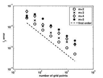
Figure 1 plots the $l_{2}$ errors between the numerical solution at time $t=20/32$ and the exact solution (38) and shows that the method is first order convergent, as expected for this choice of time stepping procedure and also due to the presence of the singularity in the first derivative of the exact solution. The dashed line is a reference slope for first order schemes. We observe that the convergence is not significantly affected by the parameter $m$.

Figure 1: $l_{2}$ error at final time for $N=32,64,\ldots,2048$, $m=2$, final time $t=20/32$, $\mathrm{\Delta}t=h$.

(a)	(b)

Figure 2: Average, minimum and maximum number of Newton iterations performed during the integration until final time. In (a) $\mathrm{\Delta}t$ was kept fixed and $m$ varied, in (b) $m=2$ was kept fixed and $\mathrm{\Delta}t$ varied.

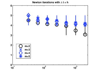
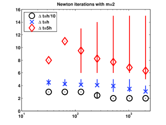
Figure 2 plots the number of Newton iterations employed by the algorithm during the integration from $t=0$ to $t=20/32$. We plot the average (circles), minimum and maximum (solid lines) number of Newton iterations per timestep. Taking $\mathrm{\Delta}t=h$ (Figure 2a), we observe that the number of Newton iterations slowly decreases when $N$ increases and that, for any given $N$ it increases only very moderately when $m$ increases. In the case $m=2$ we also tried to vary the step size from $\mathrm{\Delta}t=h/10$ to $\mathrm{\Delta}t=5h$. The results are reported in Figure 2b, showing that the number of Newton iterations grows when taking larger $\mathrm{\Delta}t$ in (2). The larger variability (for fixed $N$) and the irregular behaviour of the mean value when increasing $N$ in the case $\mathrm{\Delta}t=5h$ preludes to the loss of convergence that we observe if $\mathrm{\Delta}t$ is taken even larger.

Figure 3: History of the convergence of the Newton iterations during the first timestep. Black solid lines correspond to $m=2$ and red dashed ones to $m=3$. We show the results for $N$ ranging from $32$ to $4096$, with $\mathrm{\Delta}t=h$: the behaviour under grid refinement is indicated by the thin arrow.

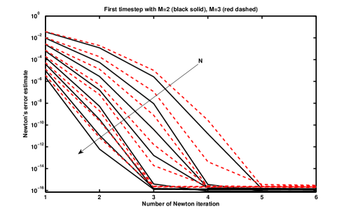
Next we verify the convergence of the Newton’s method. In Figure 3 we plot the Newton’s error estimate $\|\mathbf{u}^{1,k+1}-\mathbf{u}^{1,k}\|/\|\mathbf{u}^{1,k}\|$ obtained when computing the first timestep $\mathbf{u}^{1}$. We compare different number of grid points ($N=32,64,\ldots,4096$) as indicated by the thin arrow and two values for the exponent $m$ appearing in (37).

We emphasise that as prescribed in Proposition 2.7 the choice of $\mathrm{\Delta}t=h$ is acceptable for the convergence both of the global numerical scheme and for the convergence of the Newton procedure.

4.2 Solution of the linear system

This section is devoted to computational proposals for the solution of a linear system where the coefficient matrix is the Jacobian in (7), which is required at every step of the Newton procedure. For all the tests, we set $m=2$, final time $t=20/32$, $\mathrm{\Delta}t=h$, and we let $N$ be equal to $32,64,\ldots,1024$ for checking the optimality of the proposed best solvers.

As already stressed in Remark 2.1, the matrix is (weakly) non-symmetric so we start by considering the use of preconditioned GMRES (PGMRES).

4.2.1 GMRES

(a)	(b)

Figure 4: Average, minimum and maximum number of GMRES iterations (a) and preconditioned GMRES iterations (b) performed during the integration until final time. The dashed line in panel (a) is the least square fit.

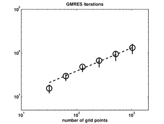
In Figure 4a we plot the average (circles), minimum and maximum (vertical lines) number of GMRES iterations performed during the integration until final time, at different spatial resolutions. A least square fit (dashed line) shows that the number of iterations grows as $N^{0.5320}$. This fact is in complete accordance with the analysis of Subsection 3.2 and in particular with equation (34).

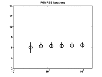
In Remark 3.5 we proved that $Y_{N}(\mathbf{u})$ is negligible with respect to the symmetric positive definite term $X_{N}(\mathbf{u})$. Accordingly, in Remark 3.6 the use of $X_{N}(\mathbf{u})$ as preconditioner for $F^{\prime}(\mathbf{u})$ was analysed and it was shown to provide a strong spectral clustering of the preconditioned matrix at $1$ and therefore we expect a number of iterations not depending on the size $N$ of the matrix as in (35): this fact is observed in practice and indeed the iteration count of the PGMRES is almost constant, with average value equal to 6 iterations (see Figure 4b).

At this point we are left with the problem of solving efficiently a generic linear system with coefficient matrix $X_{N}(\mathbf{u})$, which is a regularised version of a weighted Laplacian (i.e., by re-scaling, it is a shift of $-L_{D(\mathbf{u})}$ by $h^{2}/\mathrm{\Delta}t$ times the identity). A standard V-cycle is thus optimally convergent since $X_{N}(\mathbf{u})$ is slightly better conditioned than a standard Laplacian.

4.2.2 CG

(a)	(b)

Figure 5: Average, minimum and maximum number of CG iterations (a) and PCG iterations (b), performed during the integration until final time. The dashed line in panel (a) is the least square fit.

Since the non-symmetric part of $F^{\prime}(\mathbf{u})$ is negligible, we can try directly the solution of the whole system by using techniques such as the preconditioned CG (PCG) or the multigrid method which in theory should suffer from the loss of symmetry in the linear system.

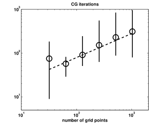
In Figure 5a we plot the average (circles), minimum and maximum (vertical lines) number of CG iterations performed during the integration until final time, at different spatial resolutions. A least square fit shows that the number of iterations grows as $N^{0.5491}$. As previously observed in connection with the GMRES method, the number of iterations is again essentially proportional to $\sqrt{N}$, which agrees with the discussion in Subsection 3.2.

However, the number of iterations for fine grids is a lot higher that the ones with GMRES (up to $950$ instead of $160$ with a grid of $1024$ points) so the latter has to be preferred.

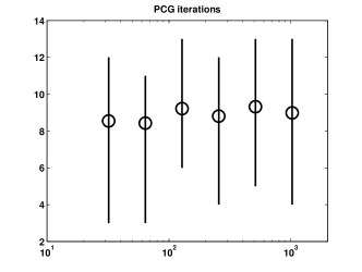
In a similar way, we consider $X_{N}(\mathbf{u})$ as preconditioner in the PCG method. Results are shown in Figure 5b. The number of iteration is again essentially constant with respect to $N$, but also in the preconditioned version, the GMRES is slightly better since the number of PCG iterations, 8 or 9, is higher that the number of PGMRES iterations which was equal to 6. Furthermore we have a higher variance in the number of iterations, due to the weak non-symmetry of whole matrix.

4.2.3 MGM

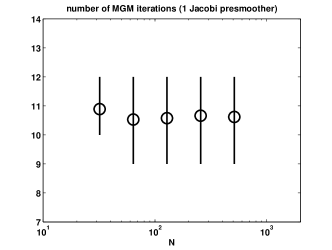
We test the optimality of MGM, as discussed in Section 3.2. We apply a single recursive call, that is the classical $V$-cycle procedure. As smoother, we use a single Jacobi step with damping factor equal to $2/3$. We observe mesh independent behaviour with 10 or 11 iterations (see Figure 6).

Figure 6: Average, minimum and maximum number of MGM iterations performed during the integration until final time.

We also tried other more sophisticated multi-iterative approaches by adding one step of post-smoother with Gauss-Seidel or standard Jacobi: the number of iterations drops to 6, but the cost per iteration is almost doubled, so that we do not observe a real advantage. The use of one step of CG or one step of GMRES as post-smoother is not better while one step of PGMRES with preconditioner equal to $X_{N}(\mathbf{u})$ reduces the number of iterations, but not enough compared with the cost of the solver needed for handling a generic system with the preconditioner as coefficient matrix.

4.2.4 Krylov methods with MGM as preconditioner

(a)	(b)

Figure 7: Average, minimum and maximum number of PGMRES (a) and PCG (b) iterations performed during the integration until final time, when using one MGM V-cycle as preconditioner.

The previous experiments confirm that the MGM is an excellent solver for our linear system. Often this method is also applied as preconditioner in a Krylov method instead of employing it as a solver. In other words, as preconditioning step, we perform a single V-cycle iteration, with the same coefficient matrix and where the datum is the residual vector at the current iteration.

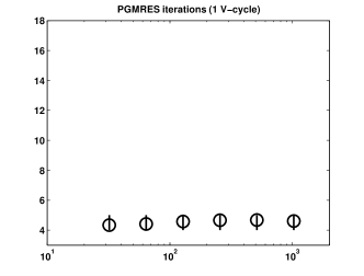
With the use of such very cheap MGM preconditioning, the PGMRES converges within 4 or 5 iterations independently of the size of the involved matrices (see Figure 7a). Comparing with the GMRES method preconditioned with the symmetric part of $F^{\prime}(\mathbf{u})$ considered in 4.2.1 and Figure 4b, the present preconditioning strategy is not only computationally cheaper, but it is also more effective since it achieves a stronger reduction of the number of GMRES iterations.

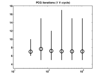
Analogously, the application of the same MGM preconditioning in the PCG method leads to a convergence within 7 or 8 iterations, again independently of the system sizes (see Figure 7b).

In conclusion, V-cycle preconditioning in connection with GMRES has to be preferred, taking into account the simplicity, the robustness (less variance in the iteration count), and the number of iterations. Indeed, due to the small iteration count, also the memory requirement does not pose any difficulty, since the number of vectors that have to be stored in the GMRES process is very reasonable.

5 2D generalization

In this section we describe a straightforward 2D generalization of the numerical approach studied in the previous part of the paper. To this end, we consider a rectangular domain $\Omega=[a_{0},a_{1}]\times[b_{0},b_{1}]\subset\mathbb{R}^{2}$ and the grid points $x_{i,j}=(a_{0}+ih,b_{0}+jk)$. For simplicity and without loss of generality, we also assume that the region $\Omega$ is square and choose identical discretization steps in the two directions (i.e. $h=k$), so that using $N$ points per direction we have $h=k=(a_{1}-a_{0})/(N+1)=(b_{1}-b_{0})/(N+1)$. The grid is thus composed of the $(N+2)^{2}$ points $x_{i,j}$ for $i$ and $j$ ranging from $0$ to $N+1$. We denote with $u_{i,j}$ the numerical value approximating $u(x_{i,j})$. Of course, as in the one-dimensional case the use of Dirichlet boundary conditions allows to reduce to gridding to the $N^{2}$ internal points.

In this setting, we generalize the finite difference discretization (3) of the differential operator as follows:

$$\left.\frac{\partial}{\partial x}\left(D(u)\frac{\partial u}{\partial x}\right)+\frac{\partial}{\partial y}\left(D(u)\frac{\partial u}{\partial y}\right)\right|_{x=x_{i,j}}\\ =\frac{D_{i+1/2,j}u_{i+1,j}-\left(D_{i+1/2,j}+D_{i-1/2,j}\right)u_{i,j}+D_{i-1/2,j}u_{i-1,j}}{h^{2}}\\ +\frac{D_{i,j+1/2}u_{i,j+1}-\left(D_{i,j+1/2}+D_{i,j-1/2}\right)u_{i,j}+D_{i,j-1/2}u_{i,j-1}}{h^{2}}+o(1),$$ (39)

where we denoted

$$D_{i+1/2,j}=\frac{D_{i+1,j}+D_{i,j}}{2}\qquad D_{i,j+1/2}=\frac{D_{i,j+1}+D_{i,j}}{2}.$$

In order to write in matrix form the approximated differential operator above, we must choose an ordering of the unknowns $u_{i,j}$, arranging them into a vector $\mathbf{u}$ and approximate

$$\left[\nabla\cdot(D(u)\nabla{u})(x_{i,j})\right]_{i,j=1}^{n}\simeq\frac{1}{h^{2}}L_{D(\mathbf{u})}\,\mathbf{u}.$$

The positions of the nonzero entries of the matrix $L_{D(\mathbf{u})}$ of course depend on the chosen ordering, so here we keep a double-index notation for the elements of $\mathbf{u}$ and of the matrix entries. Therefore, following (39), $L_{D(\mathbf{u})}$ has entries

$$\left[L_{D(\mathbf{u})}\right]_{i,j}^{l,m}=\delta_{i,l}\delta_{j,m}\left(-D_{i+1/2,j}-D_{i-1/2,j}-D_{i,j+1/2}-D_{i,j-1/2}\right)\\ +\delta_{l,i+1}\delta_{m,j}D_{i+1/2,j}+\delta_{l,i-1}\delta_{m,j}D_{i-1/2,j}\\ +\delta_{l,i}\delta_{m,j+1}D_{i,j+1/2}+\delta_{l,i}\delta_{m,j-1}D_{i,j-1/2}$$

on the $(i,j)^{\text{th}}$ row and $(l,m)^{\text{th}}$ column. The actual sparsity pattern of the resulting matrix thus depends on the ordering of the unknowns $u_{i,j}$; with the usual lexicographic ordering that has $u_{i,j}$ in the $(i+N(j-1))^{\text{th}}$ position of the vector $\mathbf{u}$, one may have, as in the case of the standard Laplacian operator, nonzero entries only on the main diagonal, on the $1^{\text{st}}$ and $N^{\text{th}}$ upper and lower diagonals.

Each timestep with the Crandall Liggett formula (2) thus requires the solution of the nonlinear equation defined by

$$F(\mathbf{u})=\mathbf{u}-\frac{\mathrm{\Delta}t}{h^{2}}L_{D(\mathbf{u})}\,\mathbf{u}-\mathbf{u}^{n-1}.$$

As in the one-dimensional case we propose to approximate the solution of the nonlinear equation with the Newton’s method; an analysis similar to that of Theorem 2.7 can be carried out in the new 2D context. The Jacobian of $F(\mathbf{u})$ is

$$F^{\prime}(\mathbf{u})=I-\frac{\mathrm{\Delta}t}{h^{2}}L_{D(\mathbf{u})}-\frac{\mathrm{\Delta}t}{h^{2}}Y(\mathbf{u})$$ (40)

where

$$Y_{i,j}^{l,m}(\mathbf{u})=\sum_{l,m}\frac{\partial\left[L_{D((\mathbf{u}))}\right]_{i,j}^{l,m}}{\partial u_{r,s}}u_{l,m}$$ (41)

with the double-index notation as above.

A tedious but straightforward computation yields

$$Y_{i,j}^{r,s}(\mathbf{u})=\frac{1}{2}D^{\prime}_{i,j}\delta_{i,r}\delta_{j,s}\left(-4u_{i,j}+u_{i+1,j}+u_{i-1,j}+u_{i,j+1}+u_{i,j-1}\right)\\ +\frac{1}{2}D^{\prime}_{i+1,j}\delta_{r,i+1}\delta_{s,j}\left(u_{i+1,j}-u_{i,j}\right)+\frac{1}{2}D^{\prime}_{i-1,j}\delta_{r,i-1}\delta_{s,j}\left(u_{i-1,j}-u_{i,j}\right)\\ +\frac{1}{2}D^{\prime}_{i,j+1}\delta_{r,i}\delta_{s,j+1}\left(u_{i,j+1}-u_{i,j}\right)+\frac{1}{2}D^{\prime}_{i,j-1}\delta_{r,i}\delta_{s,j-1}\left(u_{i,j-1}-u_{i,j}\right)$$

for the generic entry of $Y(\mathbf{u})$. (The obvious changes must be taken into account to implement the boundary conditions, e.g. either eliminating the unknowns for the points on the Dirichlet boundary or the unknowns on suitably chosen ghost points outside the Neumann boundary.)

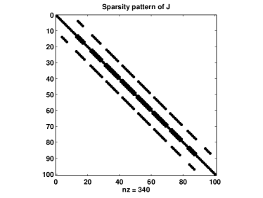(a)	(b)

Figure 8: Sparsity pattern of $Y(\mathbf{u})$ (a) and $F^{\prime}(\mathbf{u})$ (b) on a $10\times 10$ grid with the unknowns in lexicographic ordering.

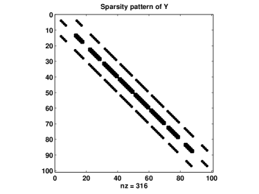
As in the one-dimensional case, the matrix $Y(\mathbf{u})$ may be written as $Y(\mathbf{u})=T(\mathbf{u})D^{\prime}(\mathbf{u})$ where $D^{\prime}(\mathbf{u})$ is a diagonal matrix with entries equal to $D^{\prime}(u_{i,j})$ and in smooth regions of the solution, the nonzero entries of $Y(\mathbf{u})$ are $O(h^{2})$ on the main diagonal and $O(h)$ outside. Moreover, entries of $Y(\mathbf{u})$ expected to be nonzero may in fact be null because the approximate solution is locally flat in a neighbourhood or because some of the $D^{\prime}(u_{k})$ may be null. When using the natural ordering of the unknowns described above, the sparsity patterns of $Y(\mathbf{u})$ and $F^{\prime}(\mathbf{u})$ for the Barenblatt solution are illustrated in figure 8. The gaps along the diagonals of $Y(\mathbf{u})$ correspond to the regions where the approximate solution $\mathbf{u}$ is flat.

Figure 9: Average, minimum and maximum number of Newton iterations performed during the integration until final time. The $3$ data series for each $N$ have been slightly shifted for clarity.

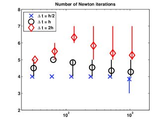
We performed our tests with the two-dimensional Barenblatt solution (see Vázquez, 2007) with exponent $m=4$ on grids of size $N\times{N}$ for $N$ ranging from $32$ to $1024$. First of all we note that the number of Newton iterations required at each timestep is almost independent of $N$ and is (on average) $4$ when $\mathrm{\Delta}t=0.5h$, $4.5$ when $\mathrm{\Delta}t=h$ and $6.5$ when $\mathrm{\Delta}t=2h$ (see Figure 9).

(a)	(b)

Figure 10: Number of GMRES iterations at different grid sizes, in 2D. (a) without preconditioning. (b) with V-cycle preconditioner. On the right, the $3$ data series for each $N$ have been slightly shifted for clarity.

We point out that the results of Section 3.1 generalize to the two-dimensional case and thus we perform numerical tests using a multigrid iteration as preconditioner for PGMRES which in Section 4 provided best results in the one dimensional case.

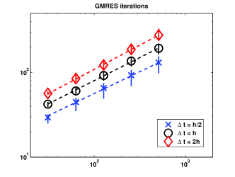
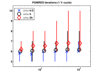
In particular we employ a single V-cycle iteration, with a Galerkin approach using the bilinear interpolation as prolongation operator and one step of red-black Gauss-Seidel as pre-smoother. In Figure 10 we plot the mean (symbols) and minimum-maximum (solid lines) number of GMRES iterations needed at different spatial resolutions. Different colours correspond to different choices of $\mathrm{\Delta}t$, namely $\mathrm{\Delta}t=h/2$ (blue crosses), $\mathrm{\Delta}t=h$ (black circles) and $\mathrm{\Delta}t=2h$ (red diamonds). The left panel shows that, without preconditioning, the number of GMRES iterations grows with the grid size: least square fits yield the approximations $N^{0.5165}$, $N^{0.5435}$ and $N^{0.5702}$ respectively for the number of GMRES iterations on an $N\times{N}$ grid with the three choices of $\mathrm{\Delta}t$ mentioned above. For homogeneity, the results for $N=1024$ are not reported in the graph, since they require the restarted GMRES method or a parallel implementation, due to memory limitations when run on a PC with 8Mb of RAM.

Figure 10b clearly demonstrates the optimality of the preconditioning strategy adopted, with the number of iterations being in the narrow range $5$–$10$ when $N$ ranges from $32$ to $1024$ and with all the three choices of the time step and with the average number of iterations being always between $5$ and $7$. We note in passing that we also employed damped Jacobi as a smoother with analogous results on the optimality, but observing a slightly higher number of iterations ($8$–$11$ on average).

6 Conclusions and future developments

The novel contribution of this paper relies in the proposal of a fully implicit numerical method for dealing with nonlinear degenerate parabolic equations, in its convergence and stability analysis, and in the study of the related computational cost. Indeed the nonlinear nature of the underlying mathematical model requires the application of a fixed point scheme. We identified the classical Newton method in which, at every step, the solution of a large, locally structured, linear system has been handled by using specialised iterative or multi-iterative solvers. In particular, we provide a spectral analysis of the relevant matrices which has been crucial for identifying appropriate preconditioned Krylov methods with efficient V-cycle preconditioners. Numerical experiments for the validation of our multi-facet analysis complement this contribution.

Among the vast range of possible applications of degenerate parabolic equations, we point out a recent one in the field of monument conservation in Semplice et al. (2009), where an approximation technique derived from the one analysed here has been successfully employed in the forecast of marble deterioration on monuments. Having in mind the application to more complicated monument geometry, we will pursue the extension of the results of this paper to the case of finite element methods for the space discretization.

References

- Alì et al. (2007) Alì, G., Furuholt, V., Natalini, R. & Torcicollo, I. (2007) A mathematical model of sulphite chemical aggression of limestones with high permeability. I. Modeling and qualitative analysis. Transp. Porous Media, 69, 109–122.
- Aregba Driollet et al. (2004) Aregba Driollet, D., Diele, F. & Natalini, R. (2004) A mathematical model for the aggression to calcium carbonate stones: numerical approximation and asymptotic analysis. SIAM J. Appl. Math., 64, 1636–1667.
- Beckermann & Serra-Capizzano (2007) Beckermann, B. & Serra-Capizzano, S. (2007) On the asymptotic spectrum of finite element matrix sequences. SIAM J. Numer. Anal., 45, 746–769 (electronic).
- Berger et al. (1979) Berger, A., Brezis, H. & Rogers, J. (1979) A numerical method for solving the problem . RAIRO numerical analysis, 13, 297–312.
- Bertaccini et al. (2005) Bertaccini, D., Golub, G. H., Serra Capizzano, S. & Tablino Possio, C. (2005) Preconditioned HSS methods for the solution of non-Hermitian positive definite linear systems and applications to the discrete convection-diffusion equation. Numer. Math., 99, 441–484.
- Bhatia (1997) Bhatia, R. (1997) Matrix analysis. Graduate Texts in Mathematics, vol. 169. New York: Springer-Verlag, pp. xii+347.
- Brézis & Pazy (1972) Brézis, H. & Pazy, A. (1972) Convergence and approximation of semigroups of nonlinear operators in Banach spaces. J. Functional Analysis, 9, 63–74.
- Cavalli et al. (2007) Cavalli, F., Naldi, G., Puppo, G. & Semplice, M. (2007) High-order relaxation schemes for non linear degenerate diffusion problems. SIAM Journal on Numerical Analysis, 45, 2098–2119.
- Clarelli et al. (2009) Clarelli, F., Giavarini, C., Natalini, R., Nitsch, C. & Santarelli, M. (2009) Mathematical models for the consolidation processes in stones. Proc. of “International Symposium: Stone Consolidation in Cultural Heritage - research and practice”. Lisbona, May 2008. to appear.
- Crandall & Liggett (1971) Crandall, M. & Liggett, T. (1971) Generation of Semi-Groups of non linear transformations on general Banach spaces. Amer. J. Math., 93, 265–298.
- Golinskii & Serra-Capizzano (2007) Golinskii, L. & Serra-Capizzano, S. (2007) The asymptotic properties of the spectrum of nonsymmetrically perturbed Jacobi matrix sequences. J. Approx. Theory, 144, 84–102.
- Golub & Van Loan (1996) Golub, G. H. & Van Loan, C. F. (1996) Matrix computations. Johns Hopkins Studies in the Mathematical Sciences, third edn. Baltimore, MD: Johns Hopkins University Press, pp. xxx+698.
- Greenbaum (1997) Greenbaum, A. (1997) Iterative methods for solving linear systems. Frontiers in Applied Mathematics, vol. 17. Philadelphia, PA: Society for Industrial and Applied Mathematics (SIAM), pp. xiv+220.
- Hackbusch (1985) Hackbusch, W. (1985) Multigrid methods and applications. Springer Series in Computational Mathematics, vol. 4. Berlin: Springer-Verlag, pp. xiv+377.
- Magenes et al. (1987) Magenes, E., Nochetto, R. H. & Verdi, C. (1987) Energy error estimates for a linear scheme to approximate nonlinear parabolic problems. RAIRO Modél. Math. Anal. Numér., 21, 655–678.
- Ortega & Rheinboldt (1970) Ortega, J. M. & Rheinboldt, W. C. (1970) Iterative solution of nonlinear equations in several variables. New York: Academic Press, pp. xx+572.
- Saad (2003) Saad, Y. (2003) Iterative methods for sparse linear systems, second edn. Philadelphia, PA: Society for Industrial and Applied Mathematics, pp. xviii+528.
- Semplice et al. (2009) Semplice, M., Donatelli, M. & Serra-Capizzano, S. (2009) Preconditioned fully implicit pde solvers for degenerate parabolic equations with applications to monument conservation. http:www.arXiv.org, 0907.2600v1.
- Serra-Capizzano (1993) Serra-Capizzano, S. (1993) Multi-iterative methods. Comput. Math. Appl., 26, 65–87.
- Serra-Capizzano (2006) Serra-Capizzano, S. (2006) The GLT class as a generalized Fourier analysis and applications. Linear Algebra Appl., 419, 180–233.
- Serra-Capizzano & Tablino-Possio (2004) Serra-Capizzano, S. & Tablino-Possio, C. (2004) Multigrid methods for multilevel circulant matrices. SIAM J. Sci. Comput., 26, 55–85 (electronic).
- Stoer & Bulirsch (2002) Stoer, J. & Bulirsch, R. (2002) Introduction to numerical analysis. Texts in Applied Mathematics, vol. 12, third edn. New York: Springer-Verlag, pp. xvi+744. Translated from the German by R. Bartels, W. Gautschi and C. Witzgall.
- Tilli (1998) Tilli, P. (1998) Locally Toeplitz sequences: spectral properties and applications. Linear Algebra Appl., 278, 91–120.
- Trottenberg et al. (2001) Trottenberg, U., Oosterlee, C. W. & Schüller, A. (2001) Multigrid. San Diego, CA: Academic Press Inc., pp. xvi+631. With contributions by A. Brandt, P. Oswald and K. Stüben.
- Varga (1962) Varga, R. S. (1962) Matrix iterative analysis. Englewood Cliffs, N.J.: Prentice-Hall Inc., pp. xiii+322.
- Vázquez (2007) Vázquez, J. L. (2007) The porous medium equation. Oxford Mathematical Monographs. Oxford: The Clarendon Press Oxford University Press, pp. xxii+624. Mathematical theory.