Constraining SUSY models with Fittino using measurements before, with and beyond the LHC

Abstract

We investigate the constraints on Supersymmetry (SUSY) arising from available precision measurements using a global fit approach. When interpreted within minimal supergravity (mSUGRA), the data provide significant constraints on the masses of supersymmetric particles (sparticles), which are predicted to be light enough for an early discovery at the Large Hadron Collider (LHC). We provide predicted mass spectra including, for the first time, full uncertainty bands. The most stringent constraint is from the measurement of the anomalous magnetic moment of the muon. Using the results of these fits, we investigate to which precision mSUGRA and more general MSSM parameters can be measured by the LHC experiments with three different integrated luminosities for a parameter point which approximately lies in the region preferred by current data. The impact of the already available measurements on these precisions, when combined with LHC data, is also studied. We develop a method to treat ambiguities arising from different interpretations of the data within one model and provide a way to differentiate between values of different digital parameters of a model (e. g. sign$(\mu)$ within mSUGRA). Finally, we show how measurements at a linear collider with up to 1 TeV centre-of-mass energy will help to improve precision by an order of magnitude.

1 Introduction

The Large Hadron Collider (LHC) will be the first collider to directly probe physics at the TeV energy scale, the Terascale. The LHC is supposed to provide first beam collisions in autumn 2009. Despite its tremendous success, the Standard Model (SM) of particle physics exhibits a number of shortcomings which – according to the belief of many – might be remedied by new physics showing up at the Terascale. One very popular extension of the SM is Supersymmetry (SUSY) Wess:1974tw . Among the virtues of SUSY are the elimination of the hierarchy problem, it can provide natural candidates to explain dark matter in the Universe and it allows for the unification of the gauge couplings at the scale of grand unification. Since no supersymmetric particles (sparticles) have been discovered to date, SUSY cannot be an exact symmetry of Nature at experimentally accessible energies. Unfortunately, the mechanism of SUSY breaking is unknown. This ignorance is efficiently parametrised in the Minimal Supersymmetric Standard Model (MSSM) Nilles:1983ge ; Haber:1984rc by the introduction of all possible soft SUSY-breaking terms into the Lagrangian with minimal sparticle content in a phenomenological way. While the most general MSSM Lagrangian introduces around 100 new parameters, mild assumptions on the absence of flavour-non-diagonal and CP-violating terms (motivated by the absence of strong flavour-changing neutral currents and electric dipole moments of the electron and neutron) and on the (effective) universality of the first two generations reduce the number of parameters to 18 (MSSM18). Still, it is a formidable experimental challenge to reconstruct 18 parameters simultaneously from future measurements. An alternative but less rigorous approach is to confront specific theoretical models of SUSY breaking (which typically reduce the number of free parameters significantly) directly with data. Among the most prominent of such models are minimal Supergravity (mSUGRA) AlvarezGaume:1983gj ; Ibanez:1982ee ; Ellis:1982wr ; Inoue:1982pi ; Chamseddine:1982jx and Gauge Mediated SUSY Breaking (GMSB) AlvarezGaume:1981wy ; Dine:1993yw ; Dine:1994vc ; Dine:1995ag .

If new phenomena which are compatible with SUSY are discovered at the LHC – which we assume in this work – one of the major challenges will be to find out the underlying model and to measure its parameters as precisely as possible. Several studies have already been performed to investigate the precision with which SUSY model parameters can be derived from measurements at the LHC and how much is gained by combining them with data from the International Linear Collider (ILC) (see e. g. Weiglein:2004hn ; Lafaye:2007vs ; Bechtle:2005vt ; Lester:2005je ). So far these studies assume an accuracy for the used observables which will only be attainable with a fairly large integrated luminosity. Thus they reflect the situation in which we might be in several years from now or – for studies including ILC measurements – even later.

In this paper we test the compatibility of various SUSY models with presently available data and constrain the corresponding parameters. Subsequently a projection of the present situation to the LHC era and beyond is performed to obtain a possible time evolution of the precision on SUSY parameters for mSUGRA and MSSM18. The fits are performed using Fittino Bechtle:2004pc version 1.5.0. The sparticle properties for a given set of Lagrangian parameters are calculated using SPheno version 3.0beta Porod:2003um which is interfaced with Fittino via the SUSY Les Houches Accord Skands:2003cj ; Allanach:2007zz . Previous work into this direction is found in Lafaye:2007vs ,Appelquist:1974tg -Flacher:2008zq .

In this paper, presently measured “low energy” (LE) observables are subjected to a global fit of the mSUGRA and GMSB model based on Markov Chain Monte Carlo techniques. To accomplish this, we take advantage of a recent compilation of up-to-date theoretical calculations of precision observables within the MSSM Buchmueller:2008qe . Also, for the first time, we combine future LHC measurements with LE observables to determine their impact in particular in the early phase of LHC data taking and within models with a large number of parameters such as the MSSM18.

This paper is organised as follows: in Section 2 we define and discuss the present and future measurements which serve as input to the global fit. We also describe briefly the computer codes employed to obtain precise theoretical predictions as a function of the SUSY parameters the data are confronted with. In Section 3, we outline in some detail the different methods used to estimate the SUSY parameters from a global $\chi^{2}$ variable. The advantages and disadvantages of the two main methods, Markov Chains and Toy Fits with Simulated Annealing, are discussed. We describe an approach to discriminate between different values for discrete parameters of the models and illustrate this approach for the parameter sign$(\mu)$ of the mSUGRA model. Also, a new method to deal with ambiguities arising from different interpretations of the data within the same model is discussed. In Section 4, the results of the different fits are presented. In Section 4.1, the constraints on mSUGRA and GMSB parameters are derived from available measurements, including observables from $K$- and $B$-decays, the anomalous magnetic moment of the muon $(g-2)_{\mu}$, precision electro-weak data from colliders and the value of the relic density of cold dark matter of the Universe, $\Omega_{\mathrm{CDM}}h^{2}$. We also determine the most sensitive observables, $(g-2)_{\mu}$ and $\Omega_{\mathrm{CDM}}h^{2}$ and show the effect of their exclusion from the fit. For the best fit point, we calculate the corresponding mass spectra of all sparticles. For the first time, the uncertainties on the parameters are converted into error bands on the sparticle masses. In Section 4.2, the results from fits to LHC data with integrated luminosities of 1, 10, 300 fb^-1 are displayed for an mSUGRA model point (SPS1a) which leads to a collider phenomenology similar to that of the best fit point. In Section 4.3, we LE data with future LHC data. We also show that by this, a stable fit of the MSSM18 can be achieved and the masses of most sparticles can be predicted. Finally, in Section 4.4 we investigate how precision measurements of sparticles at a linear electron-positron collider like the ILC with up to 1 TeV of centre-of-mass energy will turn SUSY into precision physics. The paper ends with conclusions in Section 5.

2 Measurements and Predictions

In this section, we describe the present and future experimental data which we confront with the SUSY parameter space. We use three different sets of measurements in an incremental way. These three sets are

1. ”Low energy” observables: existing experimental data which have the potential to constrain the allowed SUSY parameter space;

2. Simulated LHC measurements: expected SUSY measurements for the parameter set SPS1a at the LHC experiments ATLAS and CMS for three different integrated luminosities;

3. Simulated ILC measurements: expected SUSY measurements at the ILC running at $\sqrt{s}=500$ GeV and $\sqrt{s}=1000$ GeV.

These measurements are briefly discussed in the following sections. Finally, the codes used for the theoretical calculations are described in Section 2.4.

2.1 Low Energy Observables

While no direct evidence for SUSY particles has been found to date, these particles contribute to higher order corrections to measured physical observables in a well-defined and calculable way if SUSY is realised in Nature.

The measurements which are exploited to obtain constraints on the allowed SUSY parameter space, can be grouped in four classes:

1. Rare decays of B- and K-mesons;

2. The anomalous magnetic moment of the muon;

3. Precision measurements and the Higgs boson mass limit from high energy colliders: LEP, SLC, and Tevatron;

4. The relic density of cold dark matter in the Universe.

For reasons of comparability, the same measured values have been used for the fit as in Buchmueller:2008qe although some of them, e. g. the mass of the top quark have been updated meanwhile. The exploited measurements and their values are summarised in Table 1. In the next sections these measurements are briefly described and limitations on their interpretation in terms of SUSY are discussed.

Table 1: Available measurements from $B$-factories, kaon experiments, LEP, SLC and the Tevatron, as well as the measurement of $(g-2)_{\mu}$ and the cold dark matter relic density. Correlations amongst the electro-weak precision observables as given in :2005ema are studied for the fit to the existing measurements. No effect of the correlations on the allowed parameter regions is found.

Observable	Experimental	Uncertainty		Exp. Reference
	Value	stat	syst
${\cal B}(B\to s\gamma)/{\cal B}(B\to s\gamma)_{\mathrm{SM}}$	1.117	0.076	0.096	Barberio:2006bi
${\cal B}(B_{s}\to\mu\mu)$	$<$ 4.7$\times 10^{-8}$			Barberio:2006bi
${\cal B}(B_{d}\to\ell\ell)$	$<$ 2.3$\times 10^{-8}$			Barberio:2006bi
${\cal B}(B\to\tau\nu)/{\cal B}(B\to\tau\nu)_{\mathrm{SM}}$	1.15	0.40		Aubert:2004kz
${\cal B}(B_{s}\to X_{s}\ell\ell)/{\cal B}(B_{s}\to X_{s}\ell\ell)_{\mathrm{SM}}$	0.99	0.32		Barberio:2006bi
$\Delta m_{B_{s}}/\Delta m_{B_{s}}^{\mathrm{SM}}$	1.11	0.01	0.32	Bona:2007vi
$\frac{\Delta m_{B_{s}}/\Delta m_{B_{s}}^{\mathrm{SM}}}{\Delta m_{B_{d}}/\Delta m_{B_{d}}^{\mathrm{SM}}}$	1.09	0.01	0.16	Barberio:2006bi ; Bona:2007vi
$\Delta\epsilon_{K}/\Delta\epsilon_{K}^{\mathrm{SM}}$	0.92	0.14		Bona:2007vi
${\cal B}(K\to\mu\nu)/{\cal B}(K\to\mu\nu)_{\mathrm{SM}}$	1.008	0.014		Antonelli:2008jg
${\cal B}(K\to\pi\nu\bar{\nu})/{\cal B}(K\to\pi\nu\bar{\nu})_{\mathrm{SM}}$	$<$ 4.5			Artamonov:2008qb
$a_{\mu}^{\mathrm{exp}}-a_{\mu}^{\mathrm{\mathrm{SM}}}$	30.2$\times 10^{-10}$	8.8$\times 10^{-10}$	2.0$\times 10^{-10}$	Bennett:2004pv ; Moroi:1995yh
$\sin^{2}\theta_{\mathrm{eff}}$	0.2324	0.0012		:2005ema
$\Gamma_{Z}$	2.4952 GeV	0.0023 GeV	0.001 GeV	:2005ema
$R_{l}$	20.767	0.025		:2005ema
$R_{b}$	0.21629	0.00066		:2005ema
$R_{c}$	0.1721	0.003		:2005ema
$A_{\mathrm{fb}}(b)$	0.0992	0.0016		:2005ema
$A_{\mathrm{fb}}(c)$	0.0707	0.0035		:2005ema
$A_{b}$	0.923	0.020		:2005ema
$A_{c}$	0.670	0.027		:2005ema
$A_{l}$	0.1513	0.0021		:2005ema
$A_{\tau}$	0.1465	0.0032		:2005ema
$A_{\mathrm{fb}}(l)$	0.01714	0.00095		:2005ema
$\sigma_{\mathrm{had}}$	41.540 nb	0.037 nb		:2005ema
$m_{h}$	$>$ 114.4 GeV		3.0 GeV	Barate:2003sz ; Schael:2006cr ; Degrassi:2002fi
$\Omega_{\mathrm{CDM}}h^{2}$	0.1099	0.0062	0.012	Dunkley:2008ie
$1/\alpha_{em}$	127.925	0.016		Amsler:2008zzb
$G_{F}$	1.16637$\times 10^{-5}\mathrm{GeV}^{-2}$	0.00001$\times 10^{-5}\mathrm{GeV}^{-2}$		Amsler:2008zzb
$\alpha_{s}$	0.1176	0.0020		Amsler:2008zzb
$m_{Z}$	91.1875 GeV	0.0021 GeV		:2005ema
$m_{W}$	80.399 GeV	0.025 GeV	0.010 GeV	Amsler:2008zzb
$m_{b}$	4.20 GeV	0.17 GeV		Amsler:2008zzb
$m_{t}$	172.4 GeV	1.2 GeV		:2008vn
$m_{\tau}$	1.77684 GeV	0.00017 GeV		Amsler:2008zzb
$m_{c}$	1.27 GeV	0.11 GeV		:2005ema

2.1.1 Rare Decays of B and K mesons

A strong constraint on new physics can be derived from flavour physics experiments, especially at the $B$-factories. The reasons for that are two-fold: First, the flavour structure of the SM is remarkably exactly realised in Nature Charles:2004jd . The apparent absence of CP-violation or flavour changing neutral currents beyond the SM severely constrains models of new physics with additional flavour mixing. In this paper, we only study flavour-diagonal SUSY models which by construction fulfil these constraints. Second, the exact knowledge of branching fractions of rare decays, which are helicity suppressed or occur only at loop level with heavy particles in the loop, strongly constrains also flavour-diagonal models of new physics.

While the observables used here can be precisely measured (within the statistical limitations of the experiment), their prediction in the SM or in SUSY is often accompanied with theoretical uncertainties. The assumed systematical uncertainties on the theoretical predictions are listed in Table 1. They are added in quadrature to the experimental uncertainties. Amongst the most important constraints are the recent measurements of $B_{s}$ oscillations at the Tevatron, the branching fraction ${\cal B}(B\to\tau\nu)$ and the inclusive branching fraction of radiative penguin decays, $B\to s\gamma$ of the $B$ meson.

2.1.2 Anomalous Magnetic Moment of the Muon

Although the anomalous magnetic moment of the electron $(g-2)_{e}=2a_{e}$ is measured approximately a factor of 200 more precisely than the anomalous magnetic moment of the muon $(g-2)_{\mu}=2a_{\mu}$, the sensitivity to new physics of the anomalous magnetic moment of the muon is typically enhanced by a factor of $(m_{\mu}/m_{e})^{2}\approx 43\,000$, and represents a much stronger constraint. While its measurement is undisputed, there is ongoing debate about the exact value of the SM prediction for $(g-2)_{\mu}$. The reason is the fact that the non-perturbative contribution from the hadronic vacuum polarisation has to be extracted from other experiments such as low-energy $e^{+}e^{-}$ scattering at BES Bai:2001ct or from $\tau$ lepton decays Lautrup:1971jf ; Davier:2003pw ; Ghozzi:2003yn . Due to these uncertainties, the fit in Section 2.1 is performed with and without using $(g-2)_{\mu}$ as an observable.

2.1.3 Measurements from High Energy Colliders

The measurements of the $Z$ boson mass and width and of its couplings to left- and right-handed fermions in production and decay, the hadronic cross-section on the $Z$ pole, and the $W$ boson and top quark mass serve to constrain the properties of particles contributing at loop level. Due to their high precision and due the absence of any ambiguity in the interpretation of the measurement (as e. g. in the case of the relic density of cold dark matter) these measurements represent an important input to the fit.

As outlined in :2005ema , there are correlations within the LEP and SLD asymmetry measurements in the heavy flavour sector, respectively, and within the $Z$ pole observables. The effect of these correlations on the SUSY fit results have been tested for the baseline fit to the measurements from Table 1 as outlined in Section 4.1.1.

In addition and for completeness, we also use the measurements of the bottom and charm quark and tau lepton masses and the measurement of the strong coupling constant $\alpha_{s}$ as input to the fit.

2.1.4 Limit on the SM Higgs Boson Mass

The exclusion of a Higgs boson with SM-like properties below $m_{h}=114.4\,\mathrm{GeV}$ at 95% C.L. represents an important constraint on SUSY since at leading order, the lightest CP-even Higgs boson has a mass below $m_{Z}$. Only due to radiative corrections, its mass can be raised up to at most approximately 135-140 GeV Heinemeyer:1998np .

For a fit of the general MSSM to the existing data, the SM limit on the Higgs boson mass cannot be employed since for a given $m_{h}$ the gauge and Yukawa couplings of the lightest CP-even SUSY Higgs boson can deviate significantly from their SM values. Furthermore, additional decay channels, e. g. $h\to AA$ may occur.

As shown in Schael:2006cr , the experimental limits obtained for specific parameter choices can be as low as $m_{h}\geq 90$ GeV within the general CP-conserving and even lower for the CP-violating case.

In mSUGRA, however, it has been shown that such deviations cannot be realised Ellis:2001qv . For GMSB, such a general analysis is not available, but it has been checked that the model points selected by the fits in Section 4.1 do always maintain $\sin^{2}(\beta-\alpha)\approx 1$, where $\tan\beta$ is the ratio of the two Higgs vacuum expectation values and $\alpha$ the mixing angle of the two CP-even neutral Higgs bosons. This ensures a SM-like production of the lightest Higgs boson and the absence of additional decay modes such as $h\to AA$. Therefore, we can safely employ the SM limit on the Higgs boson mass in this study.

In principle, the full statistical information, i. e. $\mathrm{CL}_{s+b}(m_{h})$ on the compatibility of the search result with a SM Higgs boson of mass $m_{h}$ could be exploited and converted into a contribution to the $\chi^{2}$ function of the global fit. However, due to the theoretical uncertainty of 3 GeV on the prediction of the Higgs boson mass within SUSY, the use of this information would not have a significant impact on the results.

The recent exclusion of the SM Higgs in a small mass region around 160 GeV by the Tevatron experiments :2009pt is not considered since the SUSY models under study do not allow $m_{h}$ above approximately $135\,\mathrm{GeV}$ Heinemeyer:1998np .

2.1.5 Cold Dark Matter Relic Density

The results from the WMAP satellite on temperature fluctuations of the cosmic microwave background together with various other cosmological constraints have established a cosmological standard model, in which approximately 23 % of the total energy of the Universe is contained in cold dark matter (CDM). This is expressed in the fit in terms of $\Omega_{\mathrm{CDM}}h^{2}$. While the presence of dark matter is relatively undisputed, its nature is still unknown. If SUSY is $R$-parity conserving and the lightest SUSY particle (LSP) is neutral and sufficiently heavy to contribute to cold dark matter (or if a metastable neutral sparticle exists with a lifetime comparable to the lifetime of the Universe), it contributes to dark matter through its relic density, and it can make up all or part of the cosmologically observed dark matter. Therefore, in the fits shown later (see Section 2.1), the observable $\Omega_{\mathrm{CDM}}h^{2}$ is used in different ways or not at all as a constraint.

2.2 LHC Observables

As a case study, we assume that SUSY is realised with parameters as specified in the SPS1a parameter set of Allanach:2002nj . In Section  4.1), it will be shown that this bulk region point leads to a collider phenomenology rather similar to the best fit point obtained from low energy measurements.

For the SPS1a point, SUSY particles will be copiously produced at the LHC and a rather rich set of independent observables related to the masses and branching fractions of SUSY particles can be reconstructed. Many detailed experimental studies for this point (or phenomenologically similar points) exist.

A direct reconstruction of SUSY particle masses at the LHC is difficult due to the escaping LSPs. Therefore, where ever possible, we use observables which can be directly measured as input to the global fit. Such observables are the positions of kinematic edges and endpoint of invariant mass spectra. Where mass peaks can be reconstructed, those are used as well. Also, two ratios of branching fractions are employed.

Measured production rates are not considered in this study for two reasons: First, the prediction of rates has rather large theoretical uncertainties, in particular if the production mechanism involves the strong force. Second, the calculation of the theoretical prediction – if realistic experimental cuts are taken into account – is very time consuming since usually Monte Carlo techniques have to be used to obtain these predictions. Furthermore, the inherent statistical fluctuations of Monte Carlo predictions easily cause oscillations during the $\chi^{2}$ minimisation which destabilise the result.

Three different integrated luminosities are considered separately to define the sets of accessible observables and their statistical and systematic errors: 1 $\text{fb}^{-1}$, 10 $\text{fb}^{-1}$ and 300 $\text{fb}^{-1}$. A centre-of-mass energy of 14 TeV is assumed throughout. Most of the statistical uncertainties are taken from Weiglein:2004hn . Where ever results for the specified integrated luminosities are not available, reasonable interpolations/extrapolations are used. Dominant experimental systematic errors are expected to arise from the uncertainty of the lepton energy scale (LES) and the jet energy scale (JES). The LES uncertainty is assumed to be 0.2% for an integrated luminosity of 1 $\text{fb}^{-1}$ and 0.1% for higher integrated luminosity. For the JES uncertainty, 5% (1%) are assumed for 1 $\text{fb}^{-1}$ ($>1~{}\text{fb}^{-1}$). We assume that the energy scale uncertainties directly translate into equally large relative uncertainties on the positions of endpoints in mass spectra in case of fully leptonic or fully hadronic final states. Following Gjelsten:2004ki , half of the relative JES uncertainty is assumed as uncertainty on the endpoint for invariant mass spectra involving both leptons and jets. Uncertainties on the endpoints related to the JES and the LES are considered 100 % correlated between different measurements. Table 2 summarises all employed LHC observables together with their assumed uncertainties.

For the SPS1a point, it is possible to reconstruct sufficiently long decay chains of subsequent two-body decays, such that mass information can be extracted in a model independent way. However, it is necessary to assign the observed decay products to the correct SUSY particles from which they originate. The full combinatorics for decay chain ambiguities is not yet considered in this analysis. We assume that all decay chains are correctly identified. As a new approach to check the possible impact of misidentifications, we study the impact of a wrong assignment of an endpoint to its SUSY particles on the global fit as a case study. A more comprehensive analysis of these effects remains to be done.

Most information on SUSY particle masses within the SPS1a point can be obtained from the decay chain

$$\tilde{q}_{2}\to q\tilde{\chi}_{2}^{0}\to q\ell^{\pm}\tilde{\ell}_{R}^{\mp}\to q\ell^{+}\ell^{-}\tilde{\chi}_{1}^{0},$$ (1)

where $\ell$ denotes either electrons or muons. In total there are five different measurable invariant mass combinations possible for this decay chain: $m_{\ell\ell}^{\mathrm{max}}$, $m_{\ell\ell q}^{\mathrm{max}}$, $m_{\ell\ell q}^{\mathrm{thr}}$, $m_{\ell q\mathrm{(low)}}^{\mathrm{max}}$ and $m_{\ell q\mathrm{(high)}}^{\mathrm{max}}$ (for their definition see e. g. Gjelsten:2004ki ).

Similar to $m_{\ell\ell}^{\mathrm{max}}$, it is also possible to measure the endpoint $m_{\tau\tau}$ where the electrons/muons are replaced by tau leptons. The ratio of the total number of events in the $m_{\ell\ell}$ and the $m_{\tau\tau}$ distributions (corrected for efficiency differences) provides a measurement of

$$\frac{\mathcal{B}(\tilde{\chi}_{2}^{0}\rightarrow\tilde{\ell}_{R}\ell)\times\mathcal{B}(\tilde{\ell}_{R}\rightarrow\tilde{\chi}_{1}^{0}\ell)}{\mathcal{B}(\tilde{\chi}_{2}^{0}\rightarrow\tilde{\tau}_{1}\tau)\times\mathcal{B}(\tilde{\tau}_{1}\rightarrow\tilde{\chi}_{1}^{0}\tau)}.$$ (2)

Apart from the $m_{\ell\ell}$ endpoint there is also one additional $m_{\ell\ell}$ measurement included. It originates from $\tilde{\chi}_{4}^{0}$ decays instead of $\tilde{\chi}_{2}^{0}$. Decays of $\tilde{\chi}_{3}^{0}$ do not provide a visible $m_{\ell\ell}$ endpoint since it is mostly Higgsino for the considered benchmark point and therefore the couplings are too small. There are several $\tilde{\chi}_{4}^{0}$ decay chains providing two oppositely charged leptons. Of all possibilities, the chain is chosen which provides the largest $m_{\ell\ell}$ endpoint within the SPS1a scenario. This is the case for $\tilde{\chi}_{4}^{0}\to\ell^{\pm}\tilde{\ell}_{L}^{\mp}\to\ell^{+}\ell^{-}\tilde{\chi}_{1}^{0}$. The other endpoints are unlikely to be measurable due to the superimposed spectra from the other di-lepton decay channels.

Similar to the $\ell\to\tau$ replacement it is also possible to exchange light-flavoured jets $q$ with b-flavoured jets $b$. This yields a separate $m_{\ell\ell b}^{\text{thres}}$ measurement.

Jets which carry b-flavour also play an important role in obtaining information about the gluino mass. In SPS1a, the gluino decays via $\tilde{g}\to\tilde{q}q$ where $q$ can be any quark flavour. Due to combinatorial background, gluinos can be reconstructed best, if one focuses on

$$\tilde{g}\to b\tilde{b}_{1,2}\to bb\tilde{\chi}_{2}^{0}\to bb\ell^{\pm}\tilde{\ell}_{R}^{\mp}\to bb\ell^{+}\ell^{-}\tilde{\chi}_{1}^{0}$$ (3)

From this decay chain, the gluino mass can be reconstructed by calculating the invariant mass of the $\tilde{\chi}_{2}^{0}bb$ system, provided that the $\tilde{\chi}_{2}^{0}$ momentum is known. Due to the invisible $\tilde{\chi}_{1}^{0}$, the $\tilde{\chi}_{2}^{0}$ momentum cannot be measured directly, but in the chosen scenario it can be approximated reasonably well by Weiglein:2004hn

$$\vec{p}(\tilde{\chi}_{2}^{0})\approx\left(1-\frac{m_{\tilde{\chi}_{1}^{0}}}{m_{\ell\ell}}\right)\vec{p}_{\ell\ell}.$$ (4)

It turns out that the gluino mass estimate from this approach is highly correlated with the assumed $\tilde{\chi}_{1}^{0}$ mass, such that effectively $m_{\tilde{g}}-m_{\tilde{\chi}_{1}^{0}}$ is measured. Similarly $m_{\tilde{g}}-m_{\tilde{b}_{1}}$ and $m_{\tilde{g}}-m_{\tilde{b}_{2}}$ can be determined by measuring the difference between the invariant mass of the $\tilde{\chi}_{2}^{0}bb$ and the $\tilde{\chi}_{2}^{0}b$ system. The ratio of the total number of events in the $\tilde{b}_{1}$ and $\tilde{b}_{2}$ mass peaks can be used to determine

$$\frac{\mathcal{B}(\tilde{g}\rightarrow\tilde{b}_{2}b)\times\mathcal{B}(\tilde{b}_{2}\rightarrow\tilde{\chi}_{2}^{0}b)}{\mathcal{B}(\tilde{g}\rightarrow\tilde{b}_{1}b)\times\mathcal{B}(\tilde{b}_{1}\rightarrow\tilde{\chi}_{2}^{0}b)}.$$ (5)

The “stransverse mass” $m_{T2}$ Lester:1999tx ; Barr:2003rg is used to extract information on the $\tilde{q}_{R}$ and the $\tilde{\ell}_{L}$ mass. The exploited decay chains are $\tilde{q}_{R}\to q\tilde{\chi}_{1}^{0}$ and $\tilde{\ell}_{L}\to\ell\tilde{\chi}_{1}^{0}$, respectively. $\tilde{\ell}_{L}$ is studied in direct electro-weak di-slepton production via an s-channel Z/$\gamma$ exchange. It turns out that the endpoint of the $m_{T2}$ spectrum depends on the assumed $\tilde{\chi}_{1}^{0}$ mass in such a way that roughly $\sqrt{m_{\tilde{q}_{R}}^{2}-2m_{\tilde{\chi}_{1}^{0}}^{2}}$ and $\sqrt{m_{\tilde{\ell}_{L}}^{2}-2m_{\tilde{\chi}_{1}^{0}}^{2}}$ are measured, respectively.

Stop and sbottom sector information is obtained by a measurement of the endpoint of the invariant mass spectrum of the $tb$ system from the decay chains

$$\tilde{g} \to t\tilde{t}_{1}\to tb\tilde{\chi}_{1}^{\pm}$$ (6)

$$\tilde{g} \to b\tilde{b}_{1}\to tb\tilde{\chi}_{1}^{\pm}.$$ (7)

The variable $m_{tb}^{w}$ used in our fits is a branching fraction weighted average $m_{tb}$ endpoint for decay (6) and (7) to account for the possibility that the two endpoints might be too close to each other to be experimentally distinguishable.

To reconstruct charginos, the decay chain

$$\tilde{q}_{L}\to q\tilde{\chi}_{1}^{\pm}\to qW\tilde{\chi}_{1}^{0}\to qqq\tilde{\chi}_{1}^{0}$$ (8)

is exploited. The chargino mass is obtained from the invariant mass of the $qq\tilde{\chi}_{1}^{0}$ system where the two quarks come from the $W$ decay. The momentum of $\tilde{\chi}_{1}^{0}$ is reconstructed (up to a two-fold ambiguity) using a technique described in detail in Nojiri:2003tu .

The most precise determination of the Higgs boson mass for the considered mass range is obtained from measurements of the invariant mass of the four-lepton system in the decay $h\to ZZ\to\ell^{+}\ell^{-}\ell^{+\prime}\ell^{-\prime}$ and the di-photon mass of the decay $h\to\gamma\gamma$. The top mass is measured from a combination of several different final states and techniques, the most precise of which is a kinematic fit for the semi-leptonic final state, where one $W$ decays hadronically and the other $W$ leptonically.

Table 2: LHC observables which serve as input to the fits. The shown nominal SPS1a values have been calculated with SPheno. Most of the statistical uncertainties are taken from Weiglein:2004hn . Where numbers for the specified luminosities are not available, some interpolations/extrapolations are used. Uncertainties on the endpoints related to the jet energy scale (JES) and the lepton energy scale (LES) are considered 100 % correlated among different measurements.

Observable	Nominal	Uncertainty
	Value	1 fb-1	10 fb-1	300 fb-1	$\text{LES}_{1}$	$\text{LES}_{10,300}$	$\text{JES}_{1}$	$\text{JES}_{10,300}$	syst.
$m_{h}$	$109.6$		$1.4$	$0.1$		$0.1$
$m_{t}$	$172.4$	$1.1$	$0.05$	$0.01$			$1.5$	$1.0$
$m_{\tilde{\chi}_{1}^{\pm}}$	$180.2$			$11.4$				$1.8$
$\sqrt{m_{\tilde{\ell}_{L}}^{2}-2m_{\tilde{\chi}_{1}^{0}}^{2}}$	$148.8$			$1.7$		$0.1$			$6.0$
$m_{\tilde{g}}-m_{\tilde{\chi}_{1}^{0}}$	$507.7$		$13.7$	$2.5$				$5.1$	$10.0$
$\sqrt{m_{\tilde{q}_{R}}^{2}-2m_{\tilde{\chi}_{1}^{0}}^{2}}$	$531.0$	$19.6$	$6.2$	$1.1$			$22.7$	$4.5$	$10.0$
$m_{\tilde{g}}-m_{\tilde{b}_{1}}$	$88.7$			$1.5$				$0.9$
$m_{\tilde{g}}-m_{\tilde{b}_{2}}$	$56.8$			$2.5$				$0.6$
$m_{\ell\ell}^{\text{max}}(m_{\tilde{\chi}_{1}^{0}},m_{\tilde{\chi}_{2}^{0}},m_{\tilde{\ell}_{R}})$	$80.4$	$1.7$	$0.5$	$0.03$	$0.16$	$0.08$
$m_{\ell\ell}^{\text{max}}(m_{\tilde{\chi}_{1}^{0}},m_{\tilde{\chi}_{4}^{0}},m_{\tilde{\ell}_{L}})$	$280.6$		$12.6$	$2.3$		$0.28$
$m_{\tau\tau}^{\text{max}}(m_{\tilde{\chi}_{1}^{0}},m_{\tilde{\chi}_{2}^{0}},m_{\tilde{\tau}_{1}})$	$83.4$	$12.6$	$4.0$	$0.73$			$4.2$	$0.8$	$5.7$
$m_{\ell\ell q}^{\text{max}}(m_{\tilde{\chi}_{1}^{0}},m_{\tilde{q}_{L}},m_{\tilde{\chi}_{2}^{0}})$	$452.1$	$13.9$	$4.2$	$1.4$			$22.7$	$4.5$
$m_{\ell q}^{\text{low}}(m_{\tilde{\ell}_{R}},m_{\tilde{q}_{L}},m_{\tilde{\chi}_{2}^{0}})$	$318.6$	$7.6$	$3.5$	$0.9$			$16.2$	$3.2$
$m_{\ell q}^{\text{high}}(m_{\tilde{\chi}_{1}^{0}},m_{\tilde{\chi}_{2}^{0}},m_{\tilde{\ell}_{R}},m_{\tilde{q}_{L}})$	$396.0$	$5.2$	$4.5$	$1.0$			$19.9$	$4.0$
$m_{\ell\ell q}^{\text{thres}}(m_{\tilde{\chi}_{1}^{0}},m_{\tilde{\chi}_{2}^{0}},m_{\tilde{\ell}_{R}},m_{\tilde{q}_{L}})$	$215.6$	$26.5$	$4.8$	$1.6$			$10.8$	$2.2$
$m_{\ell\ell b}^{\text{thres}}(m_{\tilde{\chi}_{1}^{0}},m_{\tilde{\chi}_{2}^{0}},m_{\tilde{\ell}_{R}},m_{\tilde{b}_{1}})$	$195.9$		$19.7$	$3.6$				$2.0$
$m_{tb}^{\text{w}}(m_{t},m_{\tilde{t}_{1}},m_{\tilde{\chi}^{\pm}_{1}},m_{\tilde{g}},m_{\tilde{b}_{1}})$	$359.5$	$43.0$	$13.6$	$2.5$			$18.0$	$3.6$
$\frac{\mathcal{B}(\tilde{\chi}_{2}^{0}\rightarrow\tilde{\ell}_{R}\ell)\times\mathcal{B}(\tilde{\ell}_{R}\rightarrow\tilde{\chi}_{1}^{0}\ell)}{\mathcal{B}(\tilde{\chi}_{2}^{0}\rightarrow\tilde{\tau}_{1}\tau)\times\mathcal{B}(\tilde{\tau}_{1}\rightarrow\tilde{\chi}_{1}^{0}\tau)}$	$0.076$	$0.009$	$0.003$	$0.001$					$0.008$
$\frac{\mathcal{B}(\tilde{g}\rightarrow\tilde{b}_{2}b)\times\mathcal{B}(\tilde{b}_{2}\rightarrow\tilde{\chi}_{2}^{0}b)}{\mathcal{B}(\tilde{g}\rightarrow\tilde{b}_{1}b)\times\mathcal{B}(\tilde{b}_{1}\rightarrow\tilde{\chi}_{2}^{0}b)}$	$0.168$			$0.078$

2.3 ILC Observables

At a future linear electron positron collider like the ILC, a huge variety of precise measurements of SUSY particle properties from their electro-weak pair-production processes.

In this paper, in order to illustrate the potential of a linear collider, a subset of the observables used in Bechtle:2005vt is used. All expected mass measurements of Weiglein:2004hn are used together with the expected measurements of absolute Higgs branching fractions and a large variety of cross-sections times branching fraction measurements of all kinematically and statistically accessible SUSY final states. In contrast to Bechtle:2005vt , only measurements at $\sqrt{s}=500$ and $1000\,\mathrm{GeV}$ and at polarisations $(P_{e^{-}},P_{e^{+}})=(\pm 80\,\%,\mp 60\,\%)$ are used, assuming a long running time of the ILC with ${\cal L}^{\mathrm{int}}=500\,\mathrm{fb}^{-1}$ on each polarisation at $\sqrt{s}=500\,\mathrm{GeV}$ and at $\sqrt{s}=1\,\mathrm{TeV}$, respectively. The criteria used for the selection of expected cross-sections times branching fraction measurements is outlined in Bechtle:2005vt .

2.4 Theoretical Predictions

Different theoretical codes have been used for the prediction of the observables. The low energy observables are calculated by a selection of codes combined in the so-called Mastercode Buchmueller:2008qe . The RGE running of the parameters of the high-scale models down to the SUSY breaking scale are accomplished with SoftSUSY Allanach:2001kg . Subsequently, the observables of the Higgs sector and for $(g-2)_{\mu}$ are accomplished with FeynHiggs Frank:2006yh ; Heinemeyer:1998np ; Degrassi:2002fi . The flavour observables are calculated with SuperIso and other codes based on Isidori:2007jw ; Mahmoudi:2008tp . The electro-weak precision observables are derived in Heinemeyer:2006px ; Heinemeyer:2007bw and the cold dark matter relic density is calculated by Micromegas Belanger:2006is .

The SUSY mass spectrum for the LHC measurements, all direct sparticle decay branching fractions and the cross-sections for ILC are calculated with SPheno Porod:2003um .

The known systematic uncertainties for the presently available observables are included and listed in in Table 1.

Systematic uncertainties for the LHC predictions are estimated from the difference of the predictions between different RGE codes and from scale variations. The differences between RGE codes like SoftSUSY and SPheno are generally within the statistical and systematical measurements of the LHC measurements for ${\cal L}^{\mathrm{int}}=1$ and $10\,\mathrm{fb}^{-1}$, effectively making the LHC fits relatively robust against theoretical uncertainties on the order of $10-20\,\mathrm{GeV}$ Allanach:2003jw ; AguilarSaavedra:2005pw , which is in the order of magnitude of the jet energy scale uncertainties. For ${\cal L}^{\mathrm{int}}=300\,\mathrm{fb}^{-1}$ the experimental systematic uncertainties are expected to be smaller than the estimate of the theoretical uncertainties, especially in case of $m_{h}$, however improvements on the precision of the predictions can be expected until the LHC has acquired ${\cal L}^{\mathrm{int}}=300\,\mathrm{fb}^{-1}$. Theoretical uncertainties will be included for all luminosities into the fit at a later stage. Nevertheless we cross-checked the influence of an additional 3 GeV uncertainty on $m_{h}$ due to unknown higher-order corrections for some of our results and found that it does not have a significant effect on the fit results for high-scale models.

A special case is the prediction of $\Omega_{\mathrm{CDM}}h^{2}$ in GMSB models. Since the gravitino is typically a very light LSP in GMSB with a mass in the order of several MeV, it represents more hot than cold dark matter. Therefore $\Omega_{\mathrm{CDM}}h^{2}$ is not used as an observable for GMSB.

For the fits with ILC, theoretical uncertainties could play a major role, because the experimental precision assumed in Bechtle:2005vt is smaller than the current theoretical uncertainties even in the gaugino and squark sector, where uncertainties of around 1 GeV are expected Allanach:2003jw . However, the possible increase in theoretical precision until the existence of the ILC is yet unknown, hence theoretical uncertainties will be introduced into the fits with ILC at a later time.

Fittino and the calculator programs for the predictions are interfaced using the SUSY Les Houches Accord Skands:2003cj .

3 Parameter Estimation

In order to asses the consistency of a theoretical prediction (defined by a set of parameters within a specific SUSY model) for a given set of measurements the following $\chi^{2}$ is used:

$$\chi^{2}=(\vec{M}-\vec{O}(\vec{P}))^{T}\mbox{cov}_{M}^{-1}(\vec{M}-\vec{O}(\vec{P}))+\mbox{limits}.$$ (9)

Here $\vec{M}$ is a vector containing the list of measurements, $\vec{O}(\vec{P})$ a vector with the theoretical predictions for these observables for a given point in parameter space $\vec{P}$. $\mbox{cov}_{M}$ is the covariance matrix specifying the uncertainties and correlations of the measurements $\vec{M}$. In addition to the actual measurements $\vec{M}$, limits on observables can be specified (e. g. the limit on the SM Higgs mass in case of the fit of a model which ensures the presence of a SM-like Higgs boson). This is incorporated for $m$ lower (LL) or upper (UL) limits $L_{i}^{\mathrm{UL}/\mathrm{LL}}$ in the following way

$$\mbox{limits}=\sum_{i=1}^{m}\left\{\begin{array}[]{c}(O_{i}(\vec{P})-L_{i}^{\mathrm{UL}})^{2}/\sigma_{i}^{2}\quad\mbox{for}\,\,O_{i}(\vec{P})>L_{i}^{\mathrm{UL}}\\ (L_{i}^{\mathrm{LL}}-O_{i}(\vec{P}))^{2}/\sigma_{i}^{2}\quad\mbox{for}\,\,O_{i}(\vec{P})<L_{i}^{\mathrm{LL}}\\ 0\quad\mbox{for}\,\,L_{i}^{\mathrm{UL}}>O_{i}(\vec{P})>L_{i}^{\mathrm{LL}}\\ \end{array}\right.$$ (10)

where $\sigma_{i}$ specifies how steeply the limit is rising once it is reached.

Being measurements $\vec{M}$ and $\mbox{cov}_{M}^{-1}$ are independent of the theoretical model they are confronted with. Contrary to that $\vec{O}(\vec{P})$ depends on the model and it even depends on the interpretation of the data within a given model due to ambiguities in the mapping of an observed final state to its physical origin within the model (e. g. the assignment of kinematic edges in LHC mass spectra to the decays of the respective SUSY particles). The covariance matrix $\mbox{cov}_{M}$ is the sum of the statistical, systematical and theoretical covariance matrices, where the former is diagonal for independent measurements and the latter two can contain off-diagonal elements describing correlations. Using the $\chi^{2}$ expression of Equation 9, the following tasks can be addressed:

• find the absolute minimum $\chi^{2}$, i. e. the parameter point of a given model which fits the data best;

• determine the ${\cal P}$-value of the data given a best fit parameter point of a model;

• find secondary minima which could be confused with the absolute minimum;

• derive the probability that a secondary minimum of the $\chi^{2}$ surface of the exact observables in a given model turns into the absolute minimum of the experimentally observed $\chi^{2}$ surface due to statistical and systematical uncertainties of the experimental observables;

• derive the parameter uncertainties and correlations around the absolute minimum, with and without taking ambiguities in the interpretation of the data into account;

• derive the probability that due to the statistical and systematical uncertainties of the experimental data the true model of new physics is yielding a worse ${\cal P}$-value than an alternative, wrong model of new physics;

• derive predictions for most probable values of observables (and their expected variations) which are not used in the fit.

In the following, the statistical techniques used for these tasks are introduced. Their application is described and their advantages and shortcomings are discussed. We also propose an approach to estimate the uncertainties on parameters in the presence of different ambiguous interpretations of the data within the same model.

In this paper, Gaussian uncertainties are assumed both for statistical and systematic uncertainties. For systematic and theoretical uncertainties, there are other possible choices. For example, box-shaped contributions to the $\chi^{2}$ (instead of a quadratic function) are investigated elsewhere Flacher:2008zq . Given the general uncertainty on systematic and theoretical errors, we assume here that the final result does not depend on such subtle differences. In fact, a larger effect can arise from unknown correlations among the systematic and theoretical errors.

The $\chi^{2}$ hyper-surface for all considered SUSY models is highly non-trivial. As already shown in Bechtle:2004pc , gradient-based algorithms for global minimisation like MINUIT James:1975dr are insufficient for most of the problems under study. Rather more elaborate methods, based on Markov Chain Monte Carlo and Toy Fits algorithms are exploited to efficiently scan the multi-dimensional parameter space.

3.1 Minimisation and Scanning Techniques

Two different parameter estimation techniques are used in the following, a Markov Chain Monte Carlo and Toy Fits. These are briefly described in the following sections. Strong emphasis is laid on ensuring that the global minimum is found, that the errors are accurate, that the result is stable against different starting values, and that the sampling of the parameter space is fine-grained enough. This means that as many $N$-dimensional parameter combinations (where $N$ is the number of parameters of the problem) as possible are actually scanned at least within the range of $\chi^{2}-\chi^{2}_{\mathrm{min}}<6$ (approximately corresponding to the two-dimensional 95 % uncertainty interval around the best fit point). These two techniques are chosen because they are complementary in the way the uncertainties are defined and in the assumptions made for the definition of the uncertainties. An agreement in the uncertainties between the two methods provides a further strong evidence for the validity of the result.

3.1.1 Markov Chain Monte Carlo

The advantage of the Markov Chain Monte Carlo method is that it allows to obtain an efficient scan of the $\chi^{2}$ surface around its minima. Furthermore, it can be easily arranged that the sampling density in parameter space directly provides a likelihood distribution for the SUSY parameters in the Bayesian approach (see e. g. Allanach:2005kz , Allanach:2006cc ).

A Markov chain is a sequence of points $x_{i}$ $(i=1,\dots,n)$ in parameter space. Each of these points $x_{i}$ has an associated likelihood $\mathcal{L}(x_{i})$. For our study we use

$$\mathcal{L}=\exp\left(-\frac{\chi^{2}}{2}\right).$$ (11)

Using the Metropolis algorithm Metropolis:1953am , a new point $x_{n+1}$ which is randomly chosen according to a proposal probability density is added to the chain if $\mathcal{L}(x_{n+1})>\mathcal{L}(x_{n})$. Otherwise it is accepted with probability $\mathcal{L}(x_{n+1})/\mathcal{L}(x_{n})$. If the new point $x_{n+1}$ is not accepted, the old point $x_{n}$ is added to the end of the chain again and the process continues. The result is – under weak assumptions – independent of the specific choice of the proposal probability density function in the limit of infinite statistics. However, for finite statistics (even for order of 10 million parameter points for a typical 9-parameter model) the efficiency of the sampling strongly depends on the proposal distribution. Fittino implements the choice of box-shaped or Gaussian proposal distributions, where the width of the box or Gaussian can be adapted for each parameter. For each model and observable set, a set of pre-runs with several thousand points per chain is used to adapt the width parameters of each parameter individually such that the ratio of accepted and rejected points in the chain lies between $0.8$ and $1.2$, for which the best scanning efficiency is expected. This procedure takes the initial uncertainties on each parameter from the pre-run into account and is repeated manually until the result converges. For the results presented in this paper, only Gaussian proposal distributions are used.

The resulting Markov Chain can be interpreted in two different ways. In the Bayesian interpretation, it can be shown MacKay that, if the proposal probability density is properly chosen, the sampling density of points $x_{i}$ is proportional to the likelihood distribution $\mathcal{L}$, which in turn is proportional to the posterior probability in the case of flat priors (as assumed in this paper). Therefore, the best fit is obtained at the parameter point with the highest sampling density $\propto{\cal L_{\mathrm{max}}}$. The error on an individual parameter (or a subset of $D$ parameters) is derived by integrating (“marginalising”) the sampling density over all parameters apart from the parameter(s) under study. The resulting $D$-dimensional distribution can then be interpreted in terms of $-2\ln{\cal L}+2\ln{\cal L_{\mathrm{max}}}$, where ${\cal L_{\mathrm{max}}}$ is the likelihood for the parameter point with the highest likelihood. The $1\,\sigma$ uncertainty of a one-dimensional parameter distribution is defined by the region within $-2\ln{\cal L}+2\ln{\cal L_{\mathrm{max}}}=1$. In this interpretation, the marginalised $\mathcal{L}$ is the probability distribution of the true parameter value given the measurement. 68 % of this distribution is contained within $1\,\sigma$.

Figure 1: $\tan\beta$ sampling behaviour of Markov chain using LE and LHC measurements for an integrated luminosity of 1 fb^-1 within mSUGRA for two different starting points.

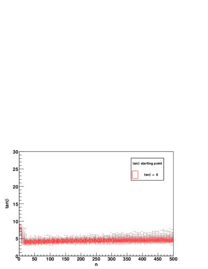
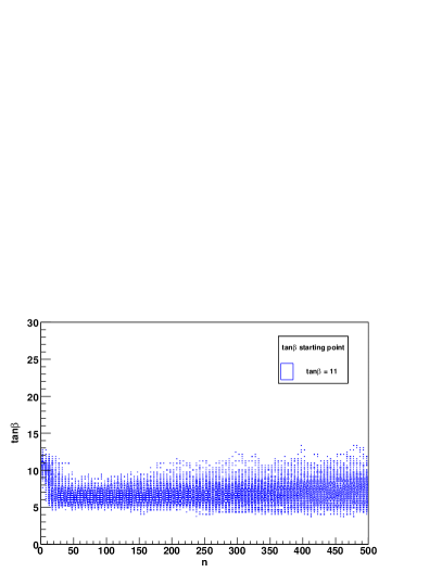
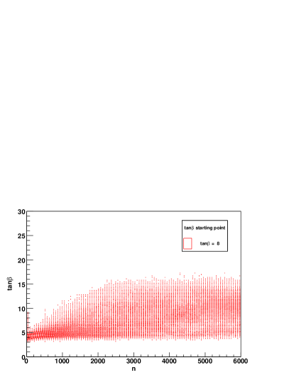
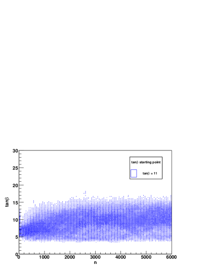
The Bayesian interpretation has to be handled with care for two independent reasons. First, the outcome can have a strong dependence on the chosen prior probability. This is e. g. exemplified in AbdusSalam:2009qd . Second, for very complex parameter spaces with many parameters (typically $8$ to $18$ in the case of the fits presented here) one needs to check carefully that the sampling has not only reached all relevant areas of the parameter space, but that in addition the sampling is completely in equilibrium, i. e. that the likelihood is really proportional to the sampling density. This problem is exemplified in Fig. 1, which shows the initial behaviour of two Markov Chains scanning same model space (mSUGRA) and the same measurements but with different starting points in the parameter $\tan\beta$. While above $n\approx 3000$ no dependence on the starting point can be observed in this example, below $n\approx 3000$ the point density is obviously not proportional to the likelihood. Therefore including this region into the calculation of the point density would distort the result unless the Markov Chain length is so large that this region has negligible impact. For all results presented in this paper which employ the Bayesian interpretation of the Markov Chain, two different starting values have been chosen. Only points for large enough $n$ are included in the chain analysis such that the projections of each parameter distribution are consistent within statistics.

While this is possible for cases with well-measured and thus strongly constraining observables and a small number of parameters (e. g. fits of a high-scale SUSY model like mSUGRA using LE and LHC measurements), this approach fails for more challenging problems like fits of an 18-dimensional more general MSSM. There are around 20 million points in a combination of several Markov Chains with different starting points. These can not be checked efficiently for the effect shown in Figure 1. Neither is it technically possible to provide sufficiently long chains due to computing limitations. Therefore, the Bayesian interpretation is used in this paper only in the case of fits of the mSUGRA model to the LHC data for illustration.

The Frequentist interpretation of the Markov Chain is used as a default in this paper. It does not make use of the sampling density directly, but employs only the obtained $\chi^{2}$ values found in the chain for each parameter point. The best fit point is directly defined by the parameter point with the lowest $\chi^{2}=\chi^{2}_{\mathrm{min}}$ (or equivalently the point with the largest likelihood $\mathcal{L}=\mathcal{L}_{\mathrm{max}}$). To obtain uncertainties for a subset of parameters this approach scans over all parameters except for those under study and chooses the scanned parameters such that $\mathcal{L}$ is maximised for each point in the studied parameter subspace. This procedure yields a profile likelihood. The $1\,\sigma\,(2\,\sigma)$ uncertainties in the one-dimensional case are defined by $\Delta\chi^{2}=\chi^{2}-\chi^{2}_{\mathrm{min}}=1\,(4)$ and, in the two-dimensional case, by $\Delta\chi^{2}=\chi^{2}-\chi^{2}_{\mathrm{min}}=2.3\,(5.99)$ BarlowBook . In the limit of Gaussian parameter distributions, i. e. a locally linear relation between measurements and parameters, the $1\,\sigma$ environment for a given set of measurements covers an area which contains the true parameter point in 68 % of all possible experimental outcomes.

This approach has several advantages over the Bayesian interpretation. First, it does not depend on prior distributions, since the likelihood in the hidden dimensions is not integrated. Instead the Markov Chain is simply used an efficient scanning technique for the parameter space: for each bin in the histogram of the parameter(s) under study the point with the lowest $\chi^{2}$ is chosen. Second, it is sufficient to scan different regions in parameter space with different granularity, as long as the obtained point density is fine enough to derive a smooth surface. This approach requires significantly less points than the Bayesian approach.

Figure 2: Frequentist interpretation of Markov chain fitting mSUGRA using only LE measurements for two different starting points.

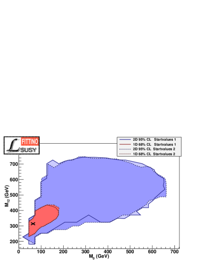
In order to test if the sampling density is sufficient to derive a smooth $\chi^{2}$ surface, the following procedure is used. For each result presented in this paper, at least two different parameter points in the parameter space are chosen as starting point. These starting points are chosen individually for each fit after an initial Markov Chain run such that they lie approximately $2\,\sigma$ away from the estimated best fit point. Then, Markov Chains are computed for each of the two starting points. An example for the comparison of the two results can be found in Figure 2. For a fit to be accepted, it is required that the differences in the shape and area of the $1\,\sigma$ and $2\,\sigma$ regions are within the differences of the binning, which is derived for each chain separately by dividing the observed $2\,\sigma$ region into $25\times 25$ bins. This procedure to ensure the robustness of the results turned out to be very important, in particular in the case of more complex fits, e. g. the MSSM fit to LE and LHC measurements and the mSUGRA fit to LE measurements. In these cases, several million sampling points turned out to be required.

The results of the Bayesian and Frequentist interpretations are compared for the case of mSUGRA fitted to LHC measurements. For more complex fits there is not enough confidence in the results of Bayesian interpretation for the reasons explained above (see also AbdusSalam:2009qd ).

As described above, the uncertainties on the model parameters can be derived from the $\Delta\chi^{2}$ values of each parameter point. It is important to note that the identification of $\Delta\chi^{2}=1$ with the $68\,\%$ uncertainty region is technically only true for problems with Gaussian uncertainties of the observables and linear dependencies between parameters and observables, hence for Gaussian parameter distributions. As visible already from Figure 2, this assumption is not fulfilled for all fits. Furthermore, for the interpretation of the fit result and especially for the derivation of conclusions on RGE running of parameters or the prediction of other observables which are not yet used in the fit, it is important to also derive correlations between the model parameters. The derivation of linear correlation coefficients can be achieved by interpreting the obtained $\chi^{2}$ surface of each combination of two parameters of the model as a numerical version of the Hesse-matrix of the problem. Normally, e. g. in MINUIT, the Hesse matrix is of course an approximation of the true $\chi^{2}$ surface. Hence the correlation coefficient can be calculated from the two-dimensional histogram of $-\Delta\chi^{2}$ for each parameter combination. For practical reasons the histogram is constrained to the region of $\Delta\chi^{2}<5.99$, corresponding to the two-dimensional $95\,\%$ uncertainty region around the best fit point. This is justified because the linear correlation coefficient are an approximation of the full non-linear correlations and are dominated by the area around the minimum.

The Frequentist analysis of the parameter space using Markov Chains could be further refined using MINUIT around the $\chi^{2}$ minimum found in the Markov Chains in order to better determine the position of the absolute minimum, independent of binning effects. However, in practice each set of Markov Chains with sufficient sampling of the $\Delta\chi^{2}<5.99$ region, as required above, ensures a sufficiently fine sampling around the absolute minimum, such that no significant improvement of a further refinement of the minimum in a MINUIT minimisation can be seen.

While Markov Chains provide a powerful tool for the study of complex parameter fits, there are a few shortcomings which make it desirable to cross-check the results with an alternative technique and to provide solutions for tasks which cannot be solved by Markov Chain Monte Carlos. First, it would be desirable to use a method which is independent of both the problem of priors (as the case in the Bayesian interpretation) or assumptions on (local) linearity of measurements and parameters (as the case in the Frequentist interpretation).

Second, the Markov Chains cannot be used to study how well a certain model can be distinguished from another model by the data, or how one interpretation of the observables is distinguished from another interpretation within the same model. Markov Chains just supply the ${\cal P}$-value of the best fit point of each model or each interpretation. They do not provide the probability to get a better ${\cal P}$-value for the “wrong” model than for the “correct” model under the assumption that one of the models is realised.

3.1.2 Toy Fits and Simulated Annealing

In addition to the Markov Chain analysis, Toy Fits are used to obtain an independent estimate of the parameter uncertainties and to compare different models or data interpretations quantitatively. The Toy Fit analysis consists of two steps. First, Markov Chains or minimisation through Simulated Annealing (for a description of the implemented algorithm of Simulated Annealing see Bechtle:2004pc ) is used to find the absolute $\chi^{2}$ minimum of a given problem. Second, Monte Carlo Toy data are created around the observables corresponding to best fit point. In the first step, the best fit parameters $\vec{P}_{o}$ are determined. Then the set of observables $\vec{M}_{o}$ corresponding to this set is calculated. This set is then used to create $N$ different MC Toy sets of pseudo-measurements $\vec{M}_{i}$ (i. e. other possible experimental outcomes which are consistent with that parameter set) by smearing around $\vec{M}_{o}$ according to the Gaussian uncertainties and correlations as defined in $\mbox{cov}_{M}$. For each of the $N$ MC Toy sets $\vec{M}_{i}$ a fit is performed using Simulated Annealing followed by a MINUIT minimisation at the minimum of the Simulated Annealing fit. This procedure yields a set of $N$ “best fit” parameter points $\vec{P}_{i}$. The distributions and correlations of $\vec{P}_{i}$ are then interpreted as the expected distributions of all possible experimental outcomes given the best fit parameter set $\vec{P}_{o}$.

In contrast to the Frequentist interpretation of the Markov Chain Monte Carlo, the uncertainties and correlations can be directly calculated from the (co-)variances of $\vec{P}_{i}$. Therefore, the results represent an estimate for the expected distribution of all possible results (including all possible non-Gaussianities). They even include possible secondary $\chi^{2}$ minima, which are turned into the absolute minimum for a subset of the observable set $\vec{M}_{i}$, where statistical and systematic uncertainties of the measurements can invert the order of the different $\chi^{2}$ minima.

Toy Fits allow for a robust cross-check of the validity of the results: For problems which are sufficiently Gaussian the distribution of the $\chi^{2}_{\mathrm{min}}$ values has to be consistent with a $\chi^{2}$ distribution for $n-m$ degrees of freedom, where $n$ is the number of observables and $m$ is the number of parameters. This criterion is checked by fitting the $\chi^{2}$ distribution to each $\chi^{2}_{\mathrm{min}}$ histogram and requiring that the fitted number of degrees of freedom agrees with the expectation for the problem within $2\,\sigma$ for a fit to be accepted.

In addition, as for Markov Chains, starting values for the parameters have been varied and the result is required to be independent of the starting value up to statistical fluctuations.

However, there is also a disadvantage of the Toy Fits with respect to the Markov Chains. In case of two different $\chi^{2}$ minima very far apart from each other (with respect to the parameter uncertainties, and with a very high $\chi^{2}$ barrier in between) which both have almost identical minimal $\chi^{2}$, one set of Toy Fits with one given starting point $\vec{P}_{s1}$ of the fits would not necessarily find both minima, requiring possibly more than two different starting points. In the limit of infinite computing power this can be overcome by starting the individual Toy Fits from randomised positions within the parameter space in order to scan for additional minima. If additional minima with acceptable ${\cal P}$-values are found and if the $\chi^{2}$ barriers between them are too high to be traversed within one minimisation, different sets of Toy Fits with starting values around the different minima can be directly treated as different models using the prescription proposed in Section 3.2. This also allows to assign a numerical value to the parameter uncertainties stemming from the different minima.

3.2 Model Discrimination and Ambiguities

All techniques discussed above are directed towards determining the uncertainties of the parameters of one model in the presence of a given set of data with one fixed interpretation of the data. In this paper a new method is proposed to use Toy Fits to solve the two remaining tasks, namely to measure how often fluctuations of the data lead to wrongly identifying a different model than the true model as the model with the best ${\cal P}$-value, and determining how ambiguities in the mapping between measurements (i.e. edges in LHC mass spectra) and predicted observables, translate into the uncertainties of the model parameters.

The first of these problems cannot be answered directly by using the ${\cal P}$-value. It represents the probability that the given experimental data are observed given a certain model with certain best fit parameters, and hence can be used to determine which models (or which interpretations of the data in a given model) are acceptable and which models are rejected by the data due to their low ${\cal P}$-value. However, it cannot be used to determine how likely it is to obtain a certain ${\cal P}$-value for a given model if the data are actually caused by another model. Such a situation can occur often for not very well constrained problems, as e. g. visible in Sections 4.1.1, 4.1.3 and 4.3.1. This question can be answered by the Toy Fits directly by fitting an arbitrary number of different models (or different interpretations of the data in the same model) $j$ with different predictions $\vec{O}(\vec{P}^{j}_{i})$ to the same set of smeared measurements $\vec{M}_{i}$. Then the probability $p_{w}$ to prefer the “wrong” models over the “correct” model, from which the observable set $\vec{M}_{o}$ is derived, can be directly determined by counting how often one of the “wrong” models achieved a better $\chi^{2}_{\mathrm{min}}$ than the “correct” model. Since in reality the “correct” model is not known, this interpretation can be repeated for each model which yields a reasonable ${\cal P}$-value. Examples using this procedure are presented in Section 4.3.1.

The second problem can be solved directly using the simultaneous Toy Fit method proposed above. The uncertainty of a model parameter is defined and measured as the square root of the variance of the parameter distribution. Each entry $\vec{P}_{i}$ in the Toy Fit parameter distributions corresponds to one individual best fit point for one model, one interpretation of the data and one individual set of smeared measurements $\vec{M}_{i}$.

In the presence of several interpretations of the data (or e. g. different possible values of a discrete parameter of the model, i. e. in all cases where different model/data combination can be fitted with the same parameters and the same measurements) the distributions of the $\vec{P}_{i}$ can be exchanged against the distribution of the $\vec{P}^{j}_{i}$, where for each smeared simulated Toy measurement $i$ the model or interpretation $j$ yielding the best fit is chosen which yields the best $\chi^{2}$. This is the natural extension of the method exploited usually in Toy Fits and described in Section 3.1.2, since in the presence of one given set of measurements $\vec{M}_{i}$ all remaining ambiguities of the interpretation of the data would be tested and for the final result the interpretation with the lowest $\chi^{2}$ (i. e. highest ${\cal P}$-value) would be chosen. The uncertainty stemming from the ambiguities is then taken into account by not citing the parameter uncertainties of the best fit interpretation of the data only, but by citing the uncertainty including the possibility that a different interpretation would have been chosen as the one with the best ${\cal P}$-value, as proposed here. Note that this interpretation naturally leaves the parameter distribution $\vec{P}_{i}$ unchanged if only one model is always yielding the best ${\cal P}$-value, i. e. if the method proposed above determines that there is 0 % probability to prefer a “wrong” model over the “correct” model. An application of this method is presented in Section 4.3.1.

4 Results

In this chapter, results are presented in terms of allowed areas in the SUSY parameter space. Also, allowed regions for SUSY particle masses are calculated from the fitted parameters.

In Section 4.1, the high-scale SUSY models mSUGRA and GMSB are tested against presently available measurements. Predictions for discovery at the LHC and the expected range of SUSY masses are presented. In Section 4.2, the constraint from LHC observables are studied alone. In Section 4.3, the expected measurements at the LHC are combined with already available observables. Here both mSUGRA and a more general 18-parameter MSSM are studied. Finally, in Section 4.4, the impact of SUSY precision measurements at the ILC together with ${\cal L}^{\mathrm{int}}=300\,\mathrm{fb}^{-1}$ of LHC data is studied, in particular for the general MSSM.

4.1 Present Low-Energy Observables

Several studies of the mSUGRA parameter space in the light of different sets of available measurements have been performed recently Buchmueller:2008qe ; AbdusSalam:2009qd . In this section, parts of these studies are repeated and extended. Emphasis is laid on understanding the impact of the most important observables on the parameter uncertainties, and on the study of the uncertainties of SUSY particle mass predictions. The methods outlined in Section 3 are used to extract parameter correlations. The impact of the SM parameters is also studied. In addition, a comparison of the predicted mSUGRA sparticle spectrum with a GMSB spectrum is presented.

In order to study the effect of the different observables, first a baseline fit with all observables from Table 1 is performed. In order to accommodate the uncertainties of the most important observables, $(g-2)_{\mu}$ in terms of its SM prediction, and $\Omega_{\mathrm{CDM}}h^{2}$ in terms of its origin, several other fits are then shown. Additionally, these observables are treated in different ways, removed one by one or removed simultaneously.

4.1.1 Fits of the mSUGRA Model

Table 3: Result of the fit of the mSUGRA model with $\mathrm{sign}(\mu)=+1$ including four additional SM parameters to all measurements listed in Table 1. The minimum $\chi^{2}$ value is $20.6$ for 22 degrees of freedom, corresponding to a ${\cal P}$-value of 54.4 %.

Parameter	Best Fit		Uncertainty
sign$(\mu)$	+1
$\alpha_{s}$	0.1177	$\pm$	0.0020
$1/\alpha_{em}$	127.924	$\pm$	0.017
$m_{Z}$ (GeV)	91.1871	$\pm$	0.0020
$m_{t}$ (GeV)	172.4	$\pm$	1.09
$\tan\,\beta$	13.2	$\pm$	7.2
$M_{1/2}$ (GeV)	331.5	$\pm$	86.6
$M_{0}$ (GeV)	76.2		${}^{+79.2}_{-29.1}$
$A_{0}$ (GeV)	383.8	$\pm$	647

The mSUGRA (or sometimes the CMSSM, which has $\mu$ as additional free continuous SUSY parameter) scenario is the best studied SUSY scenario at colliders. For the purpose of this paper, it is appealing to study it in detail using the low energy observables, since experimental studies of possible LHC measurements are available from ATLAS Aad:2009wy and CMS Ball:2007zza for several well studied mSUGRA parameter points. Knowing the allowed parameter space using the already existing observables allows the selection of a mSUGRA scenario studied at LHC which is within the currently experimentally allowed parameter region.

The baseline fit is performed using all measurements from Table 1, i. e. assuming that the current predictions for the SM contribution to $(g-2)_{\mu}$ are correct and that the cold dark matter in the Universe is entirely caused by the relic density of SUSY LSPs, which in the mSUGRA scenario has to be the lightest neutralino $\tilde{\chi}^{0}_{1}$. For all fits in this paper, if not stated otherwise, all parameter points with charged stable LSPs are excluded from the fit. The fit has been performed using the Markov Chain Monte Carlo technique described in Section 3.1.1 and applying the Frequentist interpretation. Using two different starting values of the Markov Chains, approximately 20 million points per chain have been tested with consistent results for the different starting points. The sampling density around the minimum is large enough such that an additional MINUIT minimisation is not necessary. The $\chi^{2}$ minimum of $20.6$ for 22 degrees of freedom, corresponding to a ${\cal P}$-value of 54.4 %, can be determined with good precision from the distribution of the sampled points. The ${\cal P}$-value is significantly larger than the ${\cal P}$-value of the SM fit Collaboration:2008ub of around $18\,\%$, which does not include the limits from direct Higgs searches. With the direct Higgs search limit included, the ${\cal P}$-value is $17\,\%$ Flacher:2008zq . However the analysis of the variable pulls explained below shows that this is not directly due to a better description of the SM precision variables, which cause the moderate to low ${\cal P}$-value of the SM fit. It can be seen that mSUGRA provides an excellent description of the presently available precision data.

Correlations among the observables of Table 1, as described in Section 2.1.3, are studied in a separate fit. While the minimal $\chi^{2}$ is lowered by $1.1$ due to the correlations, the results of the allowed parameter regions for the fit including correlations are identical to those of the baseline fit without correlations in the input observables. The reason for that lies in the fact that $(g-2)_{\mu}$ and $\Omega_{\mathrm{CDM}}h^{2}$ (which are uncorrelated) constrain the parameter space more strongly than any other combination of variables (see Section 4.1.2). Therefore there is no significant impact of the correlations among the electroweak precision observables.

The result of the baseline fit is given in Table 3. Due to the deviation of $(g-2)_{\mu}$ from the SM prediction towards larger values, a positive sign of $\mu$ is preferred, which is chosen for this fit. A comparison with $\mathrm{sign}(\mu)=-1$ is shown below. It can be seen that moderate values of $\tan\beta$ between 5 and 20 are preferred. The gaugino mass parameter $M_{1/2}$ is expected in the range of 200 GeV to 400 GeV, while a low scalar mass parameter $M_{0}$ between 50 GeV and 150 GeV is preferred. The universal trilinear coupling $A_{0}$ is not very well constrained and is expected to be between $-$300 GeV and 1000 GeV. As it is shown below, this region of parameter space is very favourable for early discoveries at LHC and for a rich phenomenology at ILC. In Table 3, as well as in the following tables, we quote symmetrical uncertainties whenever upper and lower uncertainties agree within 20 %, and asymmetrical uncertainties are given otherwise. It should be noted that the probability densities for the fitted parameters are usually not Gaussian, i. e. that the one-dimensional $2\,\sigma$ uncertainty at $\Delta\chi^{2}=4$ are not twice the $1\,\sigma$ uncertainty at $\Delta\chi^{2}=1$.

Note that the uncertainty of the SM parameters exactly corresponds to the uncertainties of the measurements to which the given parameter is 100 % correlated (see Table 1). This means that the direct measurement of the parameters is so precise that the additional observables from Table 1 do not play any role in their determination, which has consequences for their correlations with other parameters.

It also has to be noted that $G_{F}$ is omitted from Table 3, since $G_{F}$ is measured so precisely that virtually no effect of the inclusion of $G_{F}$ into the fit can be observed. This has been checked using a second baseline fit including $G_{F}$, which yields identical results for the other SM parameters and the mSUGRA parameters. Hence $G_{F}$ has been omitted from all subsequent fits to save computing effort. For completeness however, it is included in the discussion of the parameter correlations.

Table 4: Correlations of the mSUGRA model and the SM parameters (with $\mathrm{sign}(\mu)=+1$) using all measurements listed in Table 1. Very small correlations between SM and mSUGRA parameters is observed while there is significant correlation among the mSUGRA parameters.

Parameter	$\alpha_{s}$	$G_{F}$	$1/\alpha_{em}$	$m_{Z}$	$m_{t}$	$\tan\,\beta$	$M_{1/2}$	$M_{0}$	$A_{0}$
$\alpha_{s}$	1.000	$-$0.005	0.006	$-$0.003	$-$0.007	$-$0.003	$-$0.005	$-$0.013	$-$0.009
$G_{F}$		1.000	$-$0.003	$-$0.001	$-$0.003	$-$0.002	$-$0.022	0.007	$-$0.006
$1/\alpha_{em}$			1.000	$-$0.008	0.006	$-$0.001	$-$0.003	0.009	0.007
$m_{Z}$				1.000	$-$0.0348	0.053	0.035	0.046	0.029
$m_{t}$					1.000	0.075	0.088	0.075	0.093
$\tan\,\beta$						1.000	0.358	0.833	0.457
$M_{1/2}$							1.000	0.449	0.236
$M_{0}$								1.000	0.632
$A_{0}$									1.000

In addition to the parameter uncertainties, it is important to study the parameter correlations. Calculating uncertainties of quantities derived from the parameters does not only depend on the absolute value of the uncertainties, but also on the correlations. The prescription proposed for the calculation of correlations from Markov Chain Monte Carlos in Section 3.1.1 is used for the results in Table 4. It is interesting to note that while there are significant correlations among the mSUGRA parameters, there is no correlation in excess of $10\,\%$ between any SM parameter and any mSUGRA parameter. In addition, there are hardly any correlations among the SM parameters themselves. The reason for this is the fact that every SM parameter can be measured using an observable to which the parameter is correlated 100 %. This ensures that each SM parameter is fixed by itself to a strong precision (due to the impressive success of the SM precision measurements) without any impact of any other parameter. It should be noted however, that the correlations of Table 4 are the linear correlations of the parameters within the two-dimensional $2\,\sigma$ area. For some choices of observables (e. g. without the use of $(g-2)_{\mu}$, see below) the preferred parameter space exhibits strong non-linear correlations, restricting the reliability of this method to well-constrained fits like the baseline fit described here.

Figure 3: Pull for low energy observables used in the mSUGRA parameter fit using the observables from Table 1 and the best fit point from Table 3.

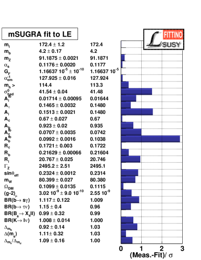
The individual pull of each observable is shown in Figure 3. Again it can be seen that the SM parameters can all be fitted individually exactly to the values of their corresponding observables. When comparing the result with the SM fits in Collaboration:2008ub ; Flacher:2008zq , the main difference is that $m_{h}$ is not a free parameter anymore, but a function of the SUSY parameters. This has the effect that the electroweak precision observables can be satisfied with a significantly larger $P$-value than for the SM fit. The preferred value of $m_{h}$ is 113.3 GeV and this is below the 95 % CL lower limit of the SM Higgs boson searches, which are applicable to mSUGRA, as outlined in Section 2.1.4. The preferred value is within 1/3 of $1\,\sigma$ of the theoretical uncertainty with respect to the 95 % CL lower limit at $m_{h}>114.4\,\mathrm{GeV}$, and even within approximately $1\,\sigma$ of the lowest mass point where the $CL_{s}$ of the combined searches is 0.5 at around $m_{h}=116.5\,\mathrm{GeV}$. The latter is corresponding to the mean value of a “measurement” of $m_{h}$, if the searches are interpreted as such Barate:2003sz .

It can be observed that apart from the change in $m_{h}$, the fit results are remarkably similar to the SM fit. This is due to the decoupling of the sparticles heavier than the electro-weak scale from the processes contributing to the precision measurements, hence rendering the result very SM-like. It can be seen that while rendering $m_{h}$ naturally heavier, mSUGRA does not mitigate the tension in some of the SM precision observables.

Figure 4: mSUGRA parameter regions compatible with relic density constraint and with all low energy measurements for various parameter combinations and sign$(\mu)$ fixed to $+1$. For both cases two-dimensional 95 % confidence level and one-dimensional 68 % confidence regions are shown. From the latter $1\,\sigma$ uncertainties for individual parameters can be derived from a projection of the area to the respective axis. The dashed lines represent the result when all observables are included. For the full lines, the measured relic dark matter density is only regarded as an upper limit of the predicted SUSY dark matter density. All other observables remain the same.

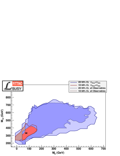
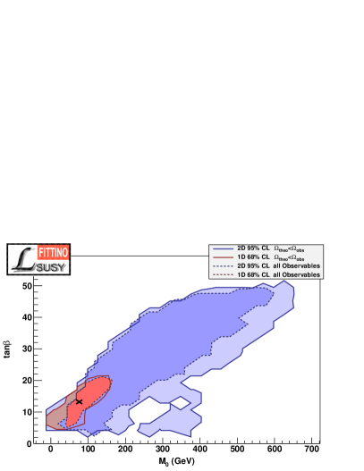
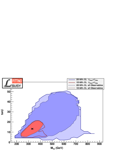
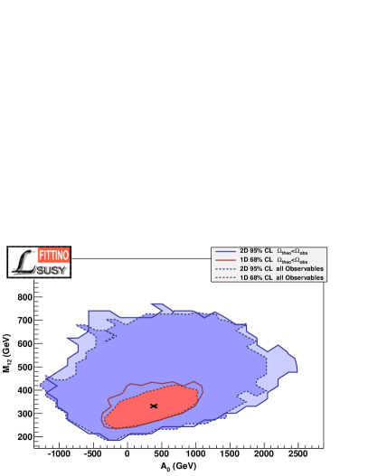
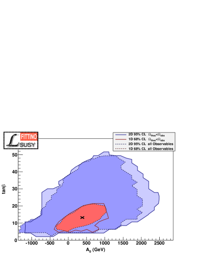
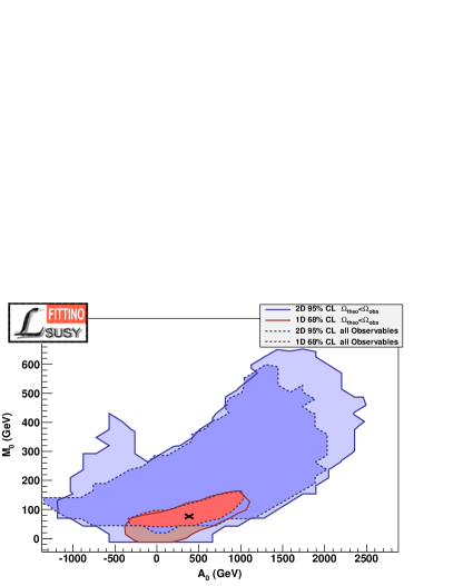
Apart from looking at the numerical results of the baseline mSUGRA fit, it is interesting to study the allowed parameter regions in detailed two-dimensional projections of each mSUGRA parameter against another parameter, as shown in the profile likelihood plots obtained using the Frequentist interpretation of the Markov Chains in Figure 4. The SM parameters have been suppressed due to their negligible correlations with themselves and with the mSUGRA parameters (see Table 4). The plots show the two-dimensional 95 % CL allowed region of the fits in blue (corresponding to $\Delta\chi^{2}=5.99$) and the one-dimensional 68 % region in red (corresponding to $\Delta\chi^{2}=1$). There are two reasons why the unusual choice of showing the $\Delta\chi^{2}=1$ curve in a two-dimensional plot has been made. First because by this the one-dimensional uncertainties of the parameters can be directly read off from the plot, which is not possible for the choice of the two-dimensional 68 % CL area at $\Delta\chi^{2}=2.3$. Second, the two-dimensional 95 % CL area gives a good indication of the experimentally allowed area, while two-dimensional 68 % CL area leaves a large room for parameter points outside the 68 % contour. The most common projection is shown in the upper left plot, which compares the allowed region in $M_{0}$ and $M_{1/2}$ between the baseline fit described above and a fit requiring only $\Omega_{\mathrm{theo}}h^{2}\leq\Omega_{\mathrm{obs}}h^{2}$, as described below in Section 4.1.2. It can be seen that on the upper left side the allowed region is directly adjacent to the excluded region where $\tilde{\tau}^{\pm}_{1}$ is the LSP, which is excluded from the fit because a stable charged LSP is in conflict with cosmological measurements. The results also show that on the $2\,\sigma$ level $M_{1/2}<800\,\mathrm{GeV}$ and $M_{0}<600\,\mathrm{GeV}$ is expected, yielding relatively light sparticles and hence good discovery prospects for the LHC. The upper right plot shows the projection of $\tan\beta$ versus $M_{0}$, showing that on the $2\,\sigma$ level $\tan\beta$ values are allowed between 3 and 50. This means that in a full simultaneous fit of all parameters $\tan\beta$ is not constrained strongly. This implies that a wide variety of different signatures is possible, as outlined in more detail below. In the middle plot on the right side it can be seen again that $A_{0}$ is not constrained very strongly, leaving a lot of room for the phenomenology of the third generation. However, this has only a small effect on the discovery prospects at LHC, since both $\tan\beta$ and $A_{0}$ have limited effects on the first two generations and the gauginos, which are most important for the discovery modes at the LHC.

Figure 5: Allowed mSUGRA parameter space from Table 3 overlaid upon the expected ATLAS discovery reach using $1~{}\mathrm{fb}^{-1}$ of data at $\sqrt{s}=14$ TeV Aad:2009wy .

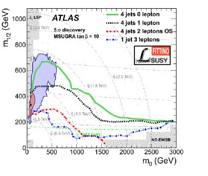
The direct comparison of the allowed parameter space of the baseline fit with the expected discovery reach of the ATLAS experiment is shown in Figure 5. The ATLAS discovery reach plot is calculated for $\tan\beta=10$ and $A_{0}=0\,\mathrm{GeV}$. Although the central values of the baseline fit of these parameters do not exactly agree with these settings, it is justified to compare the fit results with the ATLAS discovery reach plot. This is the case because first the fixed values in the discovery reach plot are within the uncertainties of the fit and second because the discovery reach depends mainly on the gluino and first generation squark masses. These are very insensitive to $A_{0}$ and not very sensitive to $\tan\beta$ due to the absence of mixing on tree level. The lines in Figure 5 correspond to the boundaries of the $5\,\sigma$ discovery region. The most sensitive search is expected to be an inclusive measurement of the effective mass spectrum of 4 jets and missing transverse energy. It can be seen that almost the entire mSUGRA parameter space allowed at 95 % CL is observable already with 1 fb^-1 of well-understood data at $\sqrt{s}=14\,\mathrm{TeV}$ of the ATLAS experiment Aad:2009wy .

Figure 6: SUSY mass spectrum as predicted by mSUGRA parameter fit to low energy measurements with sign$(\mu)$ fixed to $+1$.

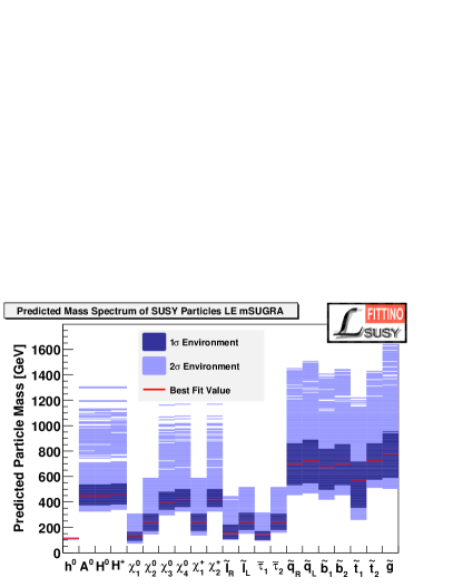
From the Markov Chain results, also the probability densities for the sparticle masses can be deduced. In Figure 6 the expected masses of the Higgs bosons and sparticles are shown for the baseline fit. The red lines indicate the masses corresponding to the best fit parameter point. The dark (light) blue regions denote the one-dimensional 68 % (95 %) CL area, corresponding to the $\Delta\chi^{2}<1$ ($\Delta\chi^{2}<4$) region around the absolute minimum. The expected spectrum shows several distinct features: The Higgs boson mass is well constrained to $m_{h}=113.3\pm 2.5\,\mathrm{GeV}$, just above the LEP exclusion bound. The lightest SUSY particle (LSP) is the stable $\tilde{\chi}^{0}_{1}$ at $m_{\tilde{\chi}^{0}_{1}}=130\pm 35\,\mathrm{GeV}$ with a relatively small mass difference to the next-to-lightest SUSY particle (NLSP) $\tilde{\tau}_{1}$ at $m_{\tilde{\tau}_{1}}=140\pm 25\,\mathrm{GeV}$, with the mass difference between NLSP and LSP being rather precisely constrained: $m_{\tilde{\tau}_{1}}-m_{\tilde{\chi}^{0}_{1}}=9.5\pm 2.5\,\mathrm{GeV}$. If mSUGRA is realised in Nature, this would provide challenging experimental conditions for precision measurements at the LHC, since the very small mass difference between NLSP and LSP would provide many final states with very soft particles, dominated by $\tau$-leptons, as the last reconstructable particles in the SUSY decay chain. In comparison with the discovery reach from Figure 5 it can be seen that mSUGRA would allow for relatively easy discovery in inclusive channels but difficult precision measurements in exclusive reconstruction of SUSY cascades.

Furthermore, all light neutralinos, charginos and sleptons are expected well below $m\approx 600\,\mathrm{GeV}$. The squarks and the gluino could be found below 1.6 TeV. The heavy Higgs bosons are expected below $m_{H/A}<1.2\,\mathrm{TeV}$ and would be challenging to discover even with more than $10\,\mathrm{fb}^{-1}$ of luminosity at the LHC, since $\tan\beta$ is not large enough Aad:2009wy .

Table 5: Result of the fit of the mSUGRA model with $\mathrm{sign}(\mu)=-1$ including four additional SM parameters to all measurements listed in Table 1. The minimum $\chi^{2}$ value is $31.1$ for 22 degrees of freedom, corresponding to a ${\cal P}$-value of 9.4 %.

Parameter	Best Fit		Uncertainty
sign$(\mu)$	$-$1
$\alpha_{s}$	0.1177	$\pm$	0.0018
$1/\alpha_{em}$	127.924	$\pm$	0.014
$m_{Z}$ (GeV)	91.188	$\pm$	0.0022
$m_{t}$ (GeV)	172.5	$\pm$	1.02
$\tan\,\beta$	9.6		${}^{+17.8}_{-4.5}$
$M_{1/2}$ (GeV)	125.1		${}^{+70.0}_{-25.1}$
$M_{0}$ (GeV)	2313.5		${}^{+622}_{-940}$
$A_{0}$ (GeV)	$-$29.1	$\pm$	2048

The baseline fit uses a fixed value of the discrete parameter $\mathrm{sign}(\mu)=+1$, since this choice is preferred by the positive deviation of the measured anomalous magnetic moment of the muon $a_{\mu}^{\mathrm{exp}}$ from the SM prediction. However, the difference in the overall agreement between the choice of $\mathrm{sign}(\mu)=+1$ and $\mathrm{sign}(\mu)=-1$ has to be assessed with a global fit to the same observables as used by the baseline fit, but for $\mathrm{sign}(\mu)=-1$. The result of the this fit (again using Markov Chains) is shown in Table 5. Due to the tension in $a_{\mu}^{\mathrm{exp}}-a_{\mu}^{\mathrm{SM}}$ of $3.4\,\sigma$, the minimal $\chi^{2}$ of the fit rises to $31.09$, corresponding to a ${\cal P}$-value of 9.4 %, compared to 54.4 % for the baseline fit. This result shows that $\mathrm{sign}(\mu)=-1$ is disfavoured but not excluded. The preferred parameter regions for both choices of $\mathrm{sign}(\mu)=-1$ show similar preferred values for $\tan\beta$ and $M_{1/2}$. For $\mathrm{sign}(\mu)=-1$, much larger values of $M_{0}$ are preferred.

Figure 7: mSUGRA parameter regions compatible with the relic density constraint and with all low energy measurements for various parameter combinations and sign$(\mu)$ fixed to $-1$. For both cases two-dimensional 95 % confidence level and one-dimensional 68 % confidence regions are shown. From the latter $1\sigma$ uncertainties for individual parameters can be derived from a projection of the area to the respective axis.

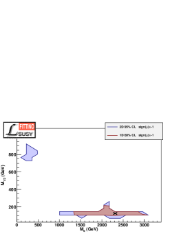
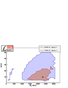
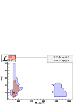
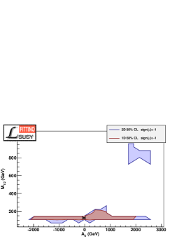
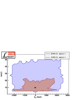
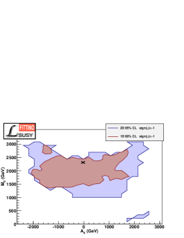
The two-dimensional projections of the mSUGRA parameters for $\mathrm{sign}(\mu)=-1$ are given in Figure 7. In contrast to the baseline fit, where one continuous two-dimensional 95 % CL area is observed, two distinct areas are found for $\mathrm{sign}(\mu)=-1$. One is located at large $M_{1/2}$ and small $M_{0}$, while the other one exhibits the opposite signature. The reason is that in both regions the negative SUSY contribution to $(g-2)_{\mu}$ is reduced, while a correct contribution to the cold dark matter relic density is preserved. The region of both large $M_{1/2}$ and $M_{0}$ is therefore cut out by the constraint of $\Omega_{\mathrm{CDM}}h^{2}$.

Figure 8: SUSY mass spectrum as predicted by mSUGRA parameter fit to low energy measurements with sign$(\mu)$ fixed to $-1$.

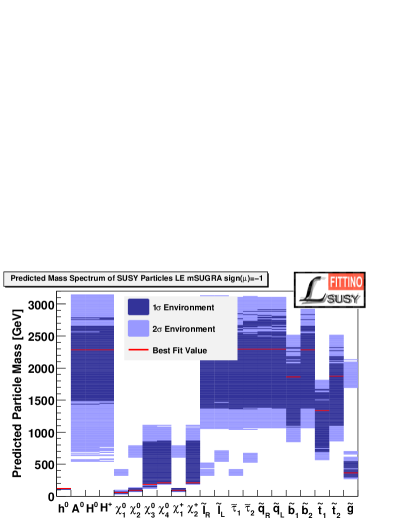
As before, the result can also be expressed in terms of the preferred sparticle masses. Fig 8 shows the best fit and the 68 % and 95 % CL areas of the observable masses for the mSUGRA fit with $\mathrm{sign}(\mu)=-1$. Since large $M_{0}$ and small $M_{1/2}$ is preferred over large $M_{1/2}$ and small $M_{0}$, as visible in Figure 7, the expected gaugino masses in this scenario are small. With $m_{\tilde{\chi}^{0}_{1}}=55^{+15}_{-10}\,\mathrm{GeV}$ a very light LSP is predicted just above the LEP mSUGRA limit of $m_{\tilde{\chi}^{0}_{1}}>47\,\mathrm{GeV}$ Heister:2003zk . In contrast to the baseline fit, heavy sleptons and squarks are expected due to the large value of $M_{0}$. The gluino is predicted to be lighter than all squarks and sleptons such that it decays via three-body decays to two jets and the LSP.

No tension between the predicted lightest Higgs boson mass with the LEP limits is present for $\mathrm{sign}(\mu)=-1$. The obtained Higgs mass value is $m_{h}=118.3\pm 3\,\mathrm{GeV}$ well above the LEP bound at $m_{h}>114.4,\mathrm{GeV}$ and also above the preferred LEP Higgs mass of $m_{h}\approx 116.5\,\mathrm{GeV}$.

Table 6: Expected branching fractions of the SUSY particles in the mSUGRA model with $\mathrm{sign}(\mu)=+1$. The results shown for the first generation are also valid for the second generation.

Decay Mode	Expected Branching Fraction	Uncertainty
$\tilde{\chi}^{0}_{2}\to\tilde{\tau}_{1}\tau$	0.46	${}^{+0.38}_{-0.44}$
$\tilde{\chi}^{0}_{2}\to\tilde{\nu}_{\tau_{1}}\nu_{\tau}$	0.076	${}^{+0.039}_{-0.067}$
$\tilde{\chi}^{0}_{2}\to\tilde{e}_{R}e$	0.040	${}^{+0.044}_{-0.038}$
$\tilde{\chi}^{0}_{2}\to\tilde{\chi}^{0}_{1}h$	0.036	${}^{+0.13}_{-0.035}$
$\tilde{\chi}^{0}_{2}\to\tilde{\chi}^{0}_{1}Z$	0.018	${}^{+0.0098}_{-0.018}$
$\tilde{\chi}^{0}_{2}\to\tilde{e}_{L}e$	0.00018	${}^{+0.14}_{-0.00018}$
$\tilde{\chi}^{0}_{2}\to\tilde{\tau}_{2}\tau$	0.	${}^{+0.014}_{-0}$
$\tilde{\chi}^{\pm}_{1}\to\tilde{\tau}_{1}\nu_{\tau}$	0.40	${}^{+0.42}_{-0.39}$
$\tilde{\chi}^{\pm}_{1}\to\tilde{\nu}_{e_{L}}e$	0.15	${}^{+0.10}_{-0.15}$
$\tilde{\chi}^{\pm}_{1}\to\tilde{\nu}_{\tau_{1}}\tau$	0.15	${}^{+0.10}_{-0.15}$
$\tilde{\chi}^{\pm}_{1}\to\tilde{\chi}^{0}_{1}W^{\pm}$	0.12	${}^{+0.079}_{-0.12}$
$\tilde{\chi}^{\pm}_{1}\to\tilde{\tau}_{2}\nu_{\tau}$	0	${}^{+0.14}_{-0}$
$\tilde{g}\to\tilde{u}_{L}u$	0.052	${}^{+0.020}_{-0.023}$
$\tilde{g}\to\tilde{u}_{R}u$	0.094	${}^{+0.030}_{-0.054}$
$\tilde{g}\to\tilde{d}_{L}d$	0.051	${}^{+0.018}_{-0.021}$
$\tilde{g}\to\tilde{d}_{R}d$	0.093	${}^{+0.031}_{-0.055}$
$\tilde{g}\to\tilde{t}_{1}t$	0.090	${}^{+0.166}_{-0.066}$
$\tilde{g}\to\tilde{t}_{2}t$	0	${}^{+0.056}_{-0}$
$\tilde{g}\to\tilde{b}_{1}b$	0.179	${}^{+0.022}_{-0.056}$
$\tilde{g}\to\tilde{b}_{2}b$	0.11	${}^{+0.009}_{-0.038}$
$\tilde{e}_{R}\to\tilde{\chi}^{0}_{1}e$	1	${}^{+0}_{-0}$
$\tilde{e}_{L}\to\tilde{\chi}^{0}_{1}e$	1	${}^{+0}_{-0.23}$
$\tilde{e}_{L}\to\tilde{\chi}^{0}_{2}e$	0	${}^{+0.085}_{-0}$
$\tilde{\tau}_{1}\to\tilde{\chi}^{0}_{1}\tau$	1	${}^{+0}_{-0}$
$\tilde{\tau}_{2}\to\tilde{\chi}^{0}_{1}\tau$	0.99	${}^{+0.011}_{-0.42}$
$\tilde{\tau}_{2}\to\tilde{\chi}^{0}_{2}\tau$	0.0007	${}^{+0.040}_{-0.0007}$
$\tilde{\tau}_{2}\to\tilde{\chi}^{\pm}_{1}\nu_{\tau}$	0.0044	${}^{+0.078}_{-0.0043}$
$\tilde{u}_{L}\to\tilde{\chi}^{0}_{1}u$	0.008	${}^{+0.0049}_{-0.0026}$
$\tilde{u}_{L}\to\tilde{\chi}^{0}_{2}u$	0.31	${}^{+0.013}_{-0.0061}$
$\tilde{u}_{L}\to\tilde{\chi}^{\pm}_{1}d$	0.64	${}^{+0.019}_{-0.0094}$
$\tilde{u}_{L}\to\tilde{\chi}^{\pm}_{2}d$	0.025	${}^{+0.0092}_{-0.018}$
$\tilde{u}_{R}\to\tilde{\chi}^{0}_{1}u$	0.99	${}^{+0.012}_{-0.0080}$
$\tilde{u}_{R}\to\tilde{\chi}^{0}_{2}u$	0.0078	${}^{+0.0064}_{-0.0072}$
$\tilde{t}_{1}\to\tilde{\chi}^{0}_{1}t$	0.18	${}^{+0.073}_{-0.037}$
$\tilde{t}_{1}\to\tilde{\chi}^{0}_{2}t$	0.15	${}^{+0.006}_{-0.069}$
$\tilde{t}_{1}\to\tilde{\chi}^{\pm}_{1}b$	0.51	${}^{+0.21}_{-0.28}$
$\tilde{t}_{1}\to\tilde{\chi}^{\pm}_{2}b$	0.15	${}^{+0.11}_{-0.15}$
$\tilde{b}_{1}\to\tilde{\chi}^{\pm}_{1}t$	0.37	${}^{+0.13}_{-0.039}$
$\tilde{b}_{1}\to\tilde{\chi}^{0}_{2}b$	0.25	${}^{+0.12}_{-0.068}$
$\tilde{b}_{1}\to\tilde{t}_{1}W^{\pm}$	0.043	${}^{+0.29}_{-0.043}$

In addition to the mass spectrum and the important mass differences, the expected dominant sparticle decay modes can be studied. A selection of branching fractions of the mSUGRA parameter points preferred by the baseline fit is shown in Table 6. The central values correspond to the best fit, the uncertainties are given by $\Delta\chi^{2}<1$ with respect to the best fit. It can be generally observed that the uncertainties of the expected branching fractions are very large, often close to 100 %. Also, there are only few sparticles with only one relevant decay mode. Therefore a rich phenomenology with many competing decay modes can be expected at the LHC. Branching fractions of the electro-weak gauginos are typically largest for the third generation, with smaller contributions from the first and second generation. In connection with the small mass difference between $m_{\tilde{\tau}_{1}}$ and $m_{\tilde{\chi}^{0}_{1}}$, the larger branching fractions into $\tau$ leptons compared to other leptons represent a challenge for the measurement of ratios of branching fractions and di-tau mass endpoints.

Following the expected decay chains, the gluino decays into squarks with a slight but not dominant preference for $\tilde{b}_{1/2}$. Generally, the branching fractions into the spartners of the right-handed degrees of freedom are larger by almost a factor of 2 than the branching fractions into the left-handed counterparts. The right squark $\tilde{q}_{R}$ decays into $\tilde{\chi}^{0}_{1}q$ almost exclusively. As expected, the decay of the $\tilde{q}_{L}$ is predicted to be more complex with decays into $\tilde{\chi}^{0}_{2}q$ and $\tilde{\chi}^{\pm}_{1}q^{\prime}$. The chargino has a preference for decays into $\tilde{\tau}_{1}\nu_{\tau}$, but includes significant contributions of decays into sneutrinos and into $\tilde{\chi}^{0}_{1}W^{\pm}$. The $\tilde{\chi}^{0}_{2}$ has a similarly rich spectrum of decays, with a dominance of $\tilde{\tau}_{1}\tau$, but with small contributions of sneutrinos, other leptons and $\tilde{\chi}^{0}_{1}h^{0}$ and $\tilde{\chi}^{0}_{1}Z^{0}$. The sleptons exhibit branching fractions of close to 100 % into $\tilde{\chi}^{0}_{1}$ and the corresponding lepton.

The results of the baseline mSUGRA fits with $\mathrm{sign}(\mu)=+1$ and $-1$ provide clear predictions for the expected measurements at the LHC. However, there are several interesting questions which remain. First, it remains to be assessed which measured observables constrain the parameter space and the regions of LHC observables in which way, i. e. which features of the measurements dominate the prediction of parameters and future observables. Second, as outlined in Section 2.1, the interpretation of some of the measurements in terms of mSUGRA is not necessarily unique. Third, alternative SUSY breaking models may predict other features for the LHC. These questions are addressed in the next sections.

4.1.2 Fits of mSUGRA to Low-Energy Observables with reduced Sets of Observables

In this section, the baseline fit with $\mathrm{sign}(\mu)=+1$ is modified by fitting the same parameters to reduced sets of observables. As described in Section 2.1, both $\Omega_{\mathrm{CDM}}h^{2}$ and $(g-2)_{\mu}$ suffer from uncertainties concerning their interpretation in terms of SUSY. In this section we show that these observables provide the strongest constraints in the parameter space, therefore the uncertainty in the interpretation of these observables has to be evaluated for the predicted parameter space and collider observables.

For $\Omega_{\mathrm{CDM}}h^{2}$ there is very little doubt about the measurement itself. However, the cosmological measurement of the cold dark matter relic density does not imply that the SUSY LSP is solely responsible for the dark matter. Therefore, we study three different possibility: First, a stable neutral SUSY LSP in the context of a $R$-parity conserving model is the only source of $\Omega_{\mathrm{CDM}}h^{2}$, and the process of the LSP production after the Big Bang and the freeze-out of the LSP is completely understood, as e. g. implemented in Belanger:2006is . This is assumed for the baseline fit in Section 4.1.1. Second, the SUSY LSP contributes to dark matter, but other unknown additional sources of dark matter are not excluded. This scenario is tested in this section by requiring that the LSP is stable and neutral and that the predicted cold dark matter relic density is smaller or equal than the observed one $\Omega_{\mathrm{theo}}h^{2}\leq\Omega_{\mathrm{obs}}h^{2}$. This still includes the assumptions that the mechanisms of CDM creation are understood. Third, additional features like a CDM creation different from the current understanding, or a meta-stable LSP, could cause differences between the measured CDM relic density and the predicted CDM relic density. The maximal effect of such uncertainties are tested by removing $\Omega_{\mathrm{CDM}}h^{2}$ from the observables in the fit.

Similarly, three different scenarios can be distinguished concerning $(g-2)_{\mu}$, where there is an ongoing debate about uncertainties on the SM prediction (see e. g. Stockinger:2008zz ; Passera:2009zz ; Jegerlehner:2009ry ; Davier:2009ag ). Therefore, in addition to the baseline fit, which uses the current mean value of measurements and the SM and SUSY prediction from Moroi:1995yh , deducing the hadronic corrections from $e^{+}e^{-}$ collision data, three other options are tested. First, in order to show the importance of the $(g-2)_{\mu}$ measurement, it is removed from the observables used in the fit. Second, it is assumed for illustration that the current deviation between SM prediction and measurement is a statistical deviation or a insufficiency in the SM prediction, i. e. that there is no visible SUSY contribution to $(g-2)_{\mu}$. Third, the prediction deducing the hadronic corrections from $\tau$ decay data Davier:2009ag is used. Several combinations of the above mentioned possibilities are studied in the following.

Table 7: Result of the fit of the mSUGRA model with $\mathrm{sign}(\mu)=+1$ including four additional SM parameters to all measurements listed in Table 1 except $\Omega_{\mathrm{CDM}}h^{2}$, for which only $\Omega_{\mathrm{\mathrm{theo}}}h^{2}\leq\Omega_{\mathrm{obs}}h^{2}$ is required. The minimum $\chi^{2}$ value is $20.4$ for 21 degrees of freedom, corresponding to a ${\cal P}$-value of 49.3 %.

Parameter	Best Fit		Uncertainty
sign$(\mu)$	+1
$\alpha_{s}$	0.1176	$\pm$	0.0025
$1/\alpha_{em}$	127.925	$\pm$	0.020
$m_{Z}$ (GeV)	91.1866	$\pm$	0.0021
$m_{t}$ (GeV)	172.2	$\pm$	1.1
$\tan\,\beta$	9.0		${}_{-3.6}^{+11.4}$
$M_{1/2}$ (GeV)	303.4		${}^{+133}_{-59.0}$
$M_{0}$ (GeV)	27.6		${}^{+122}_{-27.5}$
$A_{0}$ (GeV)	143.2		${}^{+850}_{-478}$

Since the composition of the cosmos and its dynamics are a very dynamic field of study, it is a strong assumption that only the LSP contributes to cold dark matter. Therefore, a fit of mSUGRA with the preferred choice of $\mathrm{sign}(\mu)=+1$ is performed requiring $\Omega_{\mathrm{theo}}h^{2}\leq\Omega_{\mathrm{obs}}h^{2}$ and leaving all other observables unchanged. In this fit, $\Omega_{\mathrm{theo}}h^{2}$ does not contribute to the $\chi^{2}$ for $\Omega_{\mathrm{theo}}h^{2}\leq\Omega_{\mathrm{obs}}h^{2}$ and contributes $(\Omega_{\mathrm{theo}}h^{2}-\Omega_{\mathrm{obs}}h^{2})/\sigma_{\Omega_{\mathrm{CDM}}h^{2}}$ for $\Omega_{\mathrm{theo}}h^{2}>\Omega_{\mathrm{obs}}h^{2}$. The result of this fit is shown in Table 7. The overall $\chi^{2}$ of the fit improves marginally with respect to the baseline fit. The preferred regions of $\tan\beta$, $M_{0}$ and $A_{0}$ move to slightly smaller values, but the variations are not large compared to the uncertainties. $M_{0}$ remains almost unchanged. The uncertainties increase with respect to the baseline fit, but the order of magnitude remains the same. The two-dimensional 95 % CL areas of the parameter projections are increasing, but no qualitatively new features are observed, as seen in the overlay of parameter regions with the baseline fit in Figure 4. Therefore, for this modification of the baseline fit, the predicted collider observables do not differ significantly from the baseline fit.

Figure 9: SUSY mass spectrum as predicted by mSUGRA parameter fit to low energy measurements, requiring $\Omega_{\mathrm{theo}}h^{2}\leq\Omega_{\mathrm{obs}}h^{2}$ with sign$(\mu)$ fixed to $+1$.

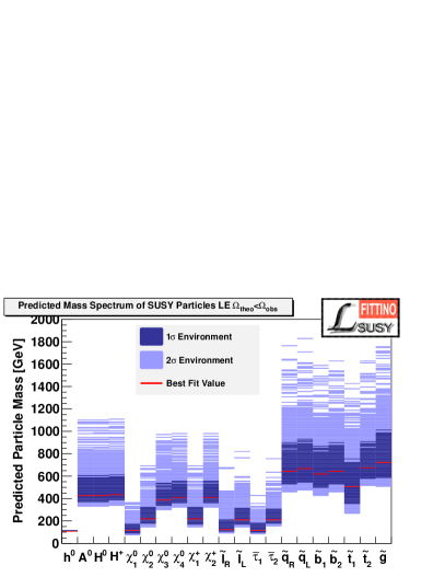
In Figure 9, the predicted Higgs boson and sparticle mass ranges are shown. The observed mass ranges are very similar to those observed in Figure 6. While the overall range of masses remains similar, there are subtle changes in the mass differences, which are explained below.

Table 8: Result of the fit of the mSUGRA model with $\mathrm{sign}(\mu)=+1$ including four additional SM parameters to all measurements listed in Table 1 except $\Omega_{\mathrm{CDM}}h^{2}$. The minimum $\chi^{2}$ value is $20.4$ for 21 degrees of freedom, corresponding to a ${\cal P}$-value of 49.3 %.

Parameter	Best Fit		Uncertainty
sign$(\mu)$	+1
$\alpha_{s}$	0.1177	$\pm$	0.0019
$1/\alpha_{em}$	127.924	$\pm$	0.014
$m_{Z}$ (GeV)	91.1870	$\pm$	0.0022
$m_{t}$ (GeV)	172.2	$\pm$	0.83
$\tan\,\beta$	10.9		${}_{-5.1}^{+9.9}$
$M_{1/2}$ (GeV)	316.2		${}_{-69.7}^{+122.9}$
$M_{0}$ (GeV)	45.1		${}_{-43.8}^{+119.3}$
$A_{0}$ (GeV)	209.1		${}_{-494.1}^{+973.5}$

Figure 10: SUSY mass spectrum as predicted by mSUGRA parameter fit to low energy measurements except $\Omega_{\mathrm{CDM}}h^{2}$ with sign$(\mu)$ fixed to $+1$.

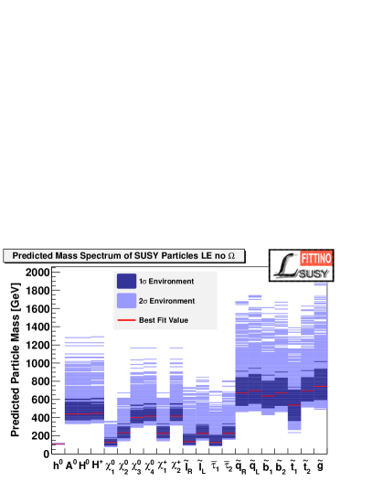
Removing $\Omega_{\mathrm{CDM}}h^{2}$ completely from the list of observables does not change the fit result significantly. The best fit point is identical within the $1\,\sigma$ uncertainty with the best fit point for $\Omega_{\mathrm{theo}}h^{2}\leq\Omega_{\mathrm{obs}}h^{2}$. The fit result is presented in Table 8. Again the uncertainties increase with respect to the baseline fit and the fit with $\Omega_{\mathrm{theo}}h^{2}\leq\Omega_{\mathrm{obs}}h^{2}$, but the order of magnitude of the results and single parameter uncertainties remain unchanged. This is exemplified in Figure 11, which shows the direct comparison of the fit results with and without $\Omega_{\mathrm{CDM}}h^{2}$. The increase in correlation through the addition of $\Omega_{\mathrm{CDM}}h^{2}$ is clearly visible. The predicted mass ranges in Figure 10 are similar to Figure 9.

Figure 11: Region in the space of the mSUGRA scenario allowed by fits with and without $\Omega_{\mathrm{CDM}}h^{2}$. It can be seen that $\Omega_{\mathrm{CDM}}h^{2}$ increases the parameter correlations, but leaves the one-dimensional projections in a similar range.

Figure 12: Region in the space of the LSP mass $m_{\tilde{\chi}^{0}_{1}}$ and $m_{\tilde{\tau}_{1}}$, which for most parameter points is the NSLP, as predicted by a mSUGRA model compatible with existing data. Using all constraints, only a area with small $m_{\mathrm{NLSP}}-m_{\mathrm{LSP}}$ remains.

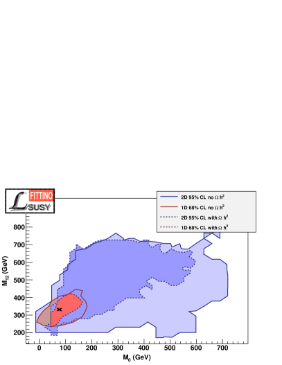
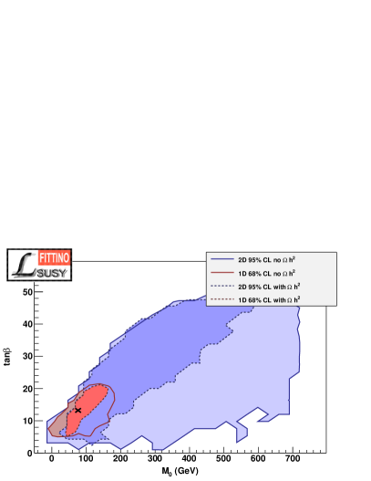
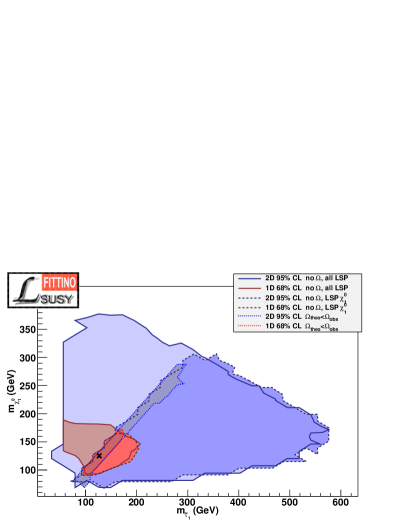
While the overall range of the accessible parameter space is not affected very strongly by including or excluding the constraint on $\Omega_{\mathrm{CDM}}h^{2}$ in the presence of the other strong observables from Table 1, there is a strong influence of $\Omega_{\mathrm{CDM}}h^{2}$ on the mass differences between the sparticles. This is shown in Figure 12 using the prediction for $m_{\tilde{\chi}^{0}_{1}}$ and $m_{\tilde{\tau}_{1}}$. If no requirements on the LSP are made at all, i. e. if also charged LSPs are allowed, a large area of chargino and stau masses are allowed. The requirement of a neutral LSP excludes the upper left area in Figure 12, where $m_{\tilde{\tau}_{1}}<m_{\tilde{\chi}^{0}_{1}}$. The remaining area is allowed without applying further constraints on $\Omega_{\mathrm{CDM}}h^{2}$. It exhibits a wide range of mass differences between LSP and NLSP, between 0 GeV and 450 GeV. The additional constraint of $\Omega_{\mathrm{theo}}h^{2}\leq\Omega_{\mathrm{obs}}h^{2}$ severely constrains this mass difference. Only a small band close to $\Omega_{\mathrm{theo}}h^{2}=\Omega_{\mathrm{obs}}h^{2}$ remains, with $m_{\tilde{\tau}_{1}}-m_{\tilde{\chi}^{0}_{1}}<22\,\mathrm{GeV}$ at 95 % CL. As already outlined in the discussion of the baseline fit, this result has significant impact on the expected exclusive collider measurements. This shows that the correlations among the parameters changes in a significant way if $\Omega_{\mathrm{CDM}}h^{2}$ is included into the fit, while the overall range of parameter uncertainties remains similar.

Table 9: Result of the Fit of the mSUGRA model with $\mathrm{sign}(\mu)=+1$ including four additional SM parameters to all measurements listed in Table 1, but with $a_{\mu}^{\mathrm{exp}}=a_{\mu}^{\mathrm{SM}}$. The minimum $\chi^{2}$ value is $19.7$ for 22 degrees of freedom, corresponding to a ${\cal P}$-value of 60.2 %.

Parameter	Best Fit		Uncertainty
sign$(\mu)$	+1
$\alpha_{s}$	0.1174	$\pm$	0.0021
$1/\alpha_{em}$	127.927	$\pm$	0.017
$m_{Z}$ (GeV)	91.1874	$\pm$	0.0020
$m_{t}$ (GeV)	172.50	$\pm$	1.19
$\tan\,\beta$	7.4		${}_{-4.6}^{+9.1}$
$M_{1/2}$ (GeV)	903.6		${}_{-778.4}^{+67.5}$
$M_{0}$ (GeV)	180.1		${}_{-110.0}^{+1566.0}$
$A_{0}$ (GeV)	956.9		${}_{-3048.3}^{+1515.6}$

The result of a mSUGRA fit to the observables from Table 1, but with $a_{\mu}^{\mathrm{exp}}=a_{\mu}^{\mathrm{SM}}$ is shown in Table 9. This shows the allowed mSUGRA parameter space for $\mathrm{sign}(\mu)=+1$ in case the difference between measurement and theoretical SM prediction of $a_{\mu}=(g-2)_{\mu}/2$ should vanish in the future, either due to statistical fluctuations or due to systematic shifts in the prediction because of a different treatment of the hadronic corrections. The preferred parameter space in this case changes dramatically with respect to the baseline fit, in contrast to the fits with different treatments of $\Omega_{\mathrm{CDM}}h^{2}$. The best fit value of $M_{1/2}$ moves to 903 GeV, but with large uncertainties towards smaller values. In contrast, the preferred value of $M_{0}$ remains small, but with very large uncertainties towards larger values. The parameter $\tan\beta$ does not change dramatically, and $A_{0}$ is basically unconstrained.

Figure 13: SUSY mass spectrum as predicted by mSUGRA parameter fit to low energy measurements with $a_{\mu}^{\mathrm{exp}}=a_{\mu}^{\mathrm{SM}}$ and with sign$(\mu)$ fixed to $+1$.

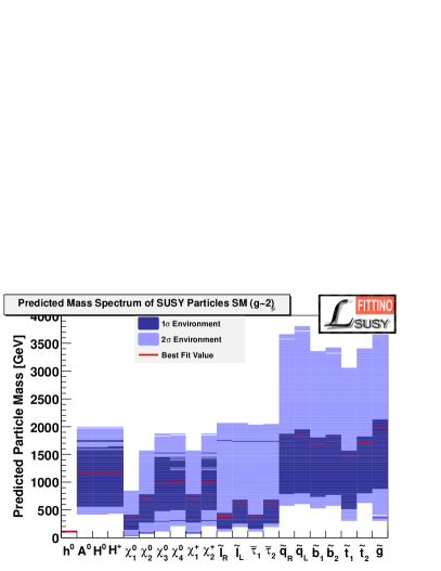
This has significant consequences for the expected sparticle masses, as shown in Figure 13. In comparison to the prediction for the baseline fit, the situation changes dramatically. The gluino and squarks tend towards masses between 500 GeV and 3500 GeV, severely reducing the expected production cross-section of colour-charged sparticles. In contrast to the heavy squarks, the slepton and electro-weak gaugino masses remain in the range below 500 GeV.

Figure 14: Expected mSUGRA parameter regions for the fit to low energy measurements with $a_{\mu}^{\mathrm{exp}}=a_{\mu}^{\mathrm{SM}}$. Results for $\mathrm{sign}(\mu)=+1$ and $\mathrm{sign}(\mu)=-1$ are overlaid. The best fit point is shown for the result with $\mathrm{sign}(\mu)=+1$

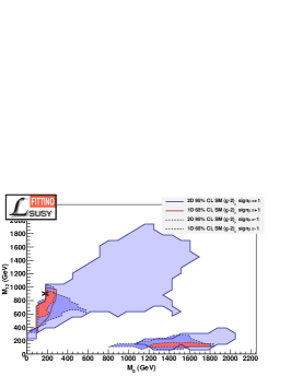
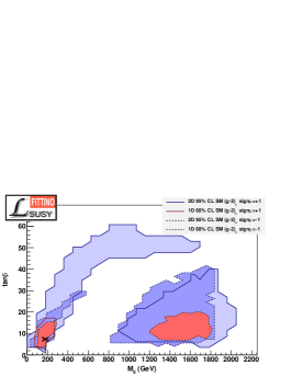
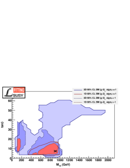
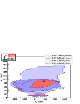
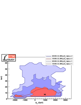
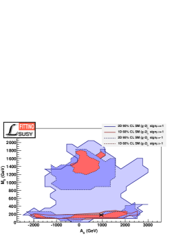
The change with respect to the baseline fit is also visible in the allowed parameter space in the detailed two-dimensional projections, as shown in Figure 14. Two distinct parameter regions both for the $1\,\sigma$ and the $2\,\sigma$ environment can be seen in several parameter projections, together with a tendency towards larger values of the mass parameters $M_{0}$ and $M_{1/2}$ and hence higher values of the expected sparticle masses, especially for the case of $\mathrm{sign}(\mu)=-1$.

Table 10: Result of the fit of the mSUGRA model with $\mathrm{sign}(\mu)=-1$ including four additional SM parameters to all measurements listed in Table 1, but with $a_{\mu}^{\mathrm{exp}}=a_{\mu}^{\mathrm{SM}}$. The minimum $\chi^{2}$ value is $19.1$ for 22 degrees of freedom, corresponding to a ${\cal P}$-value of 64.0 %.

Parameter	Best Fit		Uncertainty
sign$(\mu)$	$-$1
$\alpha_{s}$	0.1175	$\pm$	0.0018
$1/\alpha_{em}$	127.929	$\pm$	0.018
$m_{Z}$ (GeV)	91.1872	$\pm$	0.0022
$m_{t}$ (GeV)	172.25	$\pm$	1.14
$\tan\,\beta$	11.65		${}_{-7.92}^{+8.03}$
$M_{1/2}$ (GeV)	129.9		${}_{-28.8}^{+819.1}$
$M_{0}$ (GeV)	1760.1		${}_{-1654.7}^{+24.4}$
$A_{0}$ (GeV)	62.1		${}_{-2016.3}^{+2000.9}$

If the positive deviation of the measurement of $a_{\mu}$ from the SM prediction is removed, there is no remaining clear preference among the measured observables for either $\mathrm{sign}(\mu)=+1$ or $-1$. The fit of the mSUGRA scenario with $a_{\mu}^{\mathrm{exp}}=a_{\mu}^{\mathrm{SM}}$ and $\mathrm{sign}(\mu)=+1$ yields a minimal $\chi^{2}$ of $19.7$, while the fit with $\mathrm{sign}(\mu)=-1$ yields $\chi^{2}_{\mathrm{min}}=19.1$ for 22 degrees of freedom. The results of the latter fit are shown in Table 10. The best fit values of $M_{1/2}$ and $M_{0}$ are strongly different between the two results, but the uncertainties span similar areas. No significant differences are obtained for $\tan\beta$ and $A_{0}$.

Figure 15: SUSY mass spectrum as predicted by mSUGRA parameter fit to low energy measurements with $a_{\mu}^{\mathrm{exp}}=a_{\mu}^{\mathrm{SM}}$ and with sign$(\mu)$ fixed to $-1$.

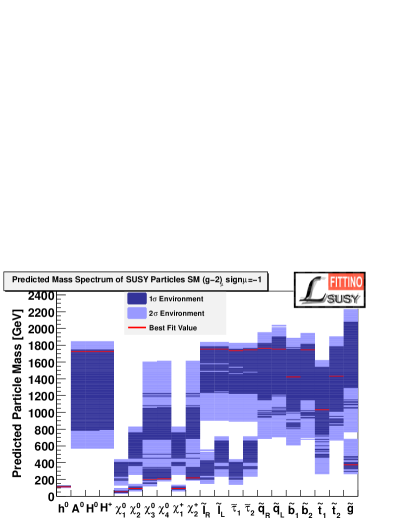
The expected sparticle masses and uncertainties for the mSUGRA fit with $a_{\mu}^{\mathrm{exp}}=a_{\mu}^{\mathrm{SM}}$ and $\mathrm{sign}(\mu)=-1$ are shown in Figure 15. In contrast to the result for $\mathrm{sign}(\mu)=+1$, very light gauginos are expected due to the low value of $M_{0}$. The best fit result for the squark masses is at around 1800 GeV at a similar level, but the uncertainty does not extend to much higher values. Especially for the sleptons there are two distinct regions predicted, which is a consequence of the prominent distinct allowed regions in the $M_{0}$ and $M_{1/2}$ distributions shown in Figure 14. Again, the gluino is expected to be lighter than the squarks, leading to decay signatures strongly different from the chain of several two-body decays expected for the baseline fit.

Table 11: Result of the fit of the mSUGRA model with $\mathrm{sign}(\mu)=+1$ including four additional SM parameters to all measurements listed in Table 1 except $(g-2)_{\mu}$. The minimum $\chi^{2}$ value is $19.47$ for 21 degrees of freedom, corresponding to a ${\cal P}$-value of 55.5 %.

Parameter	Best Fit		Uncertainty
sign$(\mu)$	+1
$\alpha_{s}$	0.1177	$\pm$	0.0019
$1/\alpha_{em}$	127.925	$\pm$	0.015
$m_{Z}$ (GeV)	91.1875	$\pm$	0.0020
$m_{t}$ (GeV)	172.5	$\pm$	1.1
$\tan\,\beta$	7.5		${}_{-4.6}^{+8.9}$
$M_{1/2}$ (GeV)	389.2		${}_{-117.5}^{+568.9}$
$M_{0}$ (GeV)	72.2		${}_{-22.1}^{+145.0}$
$A_{0}$ (GeV)	270.0		${}_{-1985.9}^{+1492.5}$

In order to explore the significance of $(g-2)_{\mu}$ for the fit result, Table 11 shows the result of the mSUGRA fit with $\mathrm{sign}(\mu)=+1$ to the observables from Table 1 excluding $(g-2)_{\mu}$. Due to the lower minimal $\chi^{2}$ of $19.5$ than the fit with $a_{\mu}^{\mathrm{exp}}=a_{\mu}^{\mathrm{SM}}$, no secondary minima are observed, therefore smaller allowed regions in $M_{0}$ are obtained for the fit without $a_{\mu}^{\mathrm{exp}}$ than with $a_{\mu}^{\mathrm{exp}}=a_{\mu}^{\mathrm{SM}}$. The comparison of Table 11 with the results of the baseline fit in Table 3 shows that $(g-2)_{\mu}$ represents an important constraint, but that the remaining observables still favour SUSY in the mass range below 1 TeV.

Table 12: Result of the fit of the mSUGRA model with $\mathrm{sign}(\mu)=+1$ including four additional SM parameters to all measurements listed in Table 1, using the predicted SM-value of $(g-2)_{\mu}$ from Davier:2009ag . The minimum $\chi^{2}$ value is $19.6$ for 22 degrees of freedom, corresponding to a ${\cal P}$-value of 60.6 %. The fit results of the SM parameters are consistent with the other fits in this section.

Parameter	Best Fit		Uncertainty
sign$(\mu)$	+1
$\tan\,\beta$	7.9		${}_{-3.9}^{+10.6}$
$M_{1/2}$ (GeV)	350.3		${}_{-79.0}^{+331.06}$
$M_{0}$ (GeV)	65.9		${}_{-15.8}^{+123.8}$
$A_{0}$ (GeV)	100.4		${}_{-852.6}^{+1435.1}$

Figure 16: SUSY mass spectrum as predicted by mSUGRA parameter fit to low energy measurements using the predicted SM-value of $(g-2)_{\mu}$ from Davier:2009ag with sign$(\mu)$ fixed to $+1$.

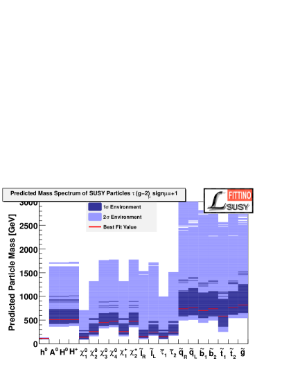
For illustration of the difference between the SM predictions of $(g-2)_{\mu}$ from $e^{+}e^{-}$ and $\tau$ data, the fit of mSUGRA using the predicted SM value and uncertainties from Davier:2009ag is shown in Table 12 and the corresponding mass spectrum in Figure 16. The mean value of the sparticle masses and mSUGRA parameters is compatible with the result of the baseline fit within their uncertainties, but the 95 % CL area of the predicted sparticle masses ranges up to around 3 TeV, in contrast to the baseline fit wit hits upper limit at 1.6 TeV at 95 % CL.

Figure 17: mSUGRA parameter regions compatible with all low energy measurements except (a) $(g-2)_{\mu}$ and (b) $\Omega_{\mathrm{CDM}}h^{2}$ for various parameter combinations and sign$(\mu)$ fixed to $+1$. For both cases two-dimensional 95 % confidence level and one-dimensional 68 % confidence regions are shown. From the latter $1\sigma$ uncertainties for individual parameters can be derived from a projection of the area to the respective axis.

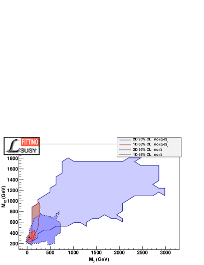
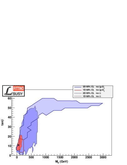
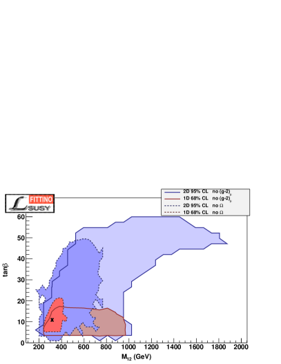
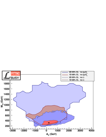
The impact of the two most stringent observables $\Omega_{\mathrm{CDM}}h^{2}$ and $(g-2)_{\mu}$ is compared in Figure 17. The dark blue areas indicate the two-dimensional 95 % CL allowed parameter region for the fit without $\Omega_{\mathrm{CDM}}h^{2}$, showing that the remaining observables constrain the allowed mSUGRA parameter space to regions below 700 GeV both in $M_{0}$ and $M_{1/2}$, accesible at LHC. The light blue region indicates the allowed parameter space for the fit without $(g-2)_{\mu}$. It can be seen that the two constraints are complementary. Without $(g-2)_{\mu}$ significantly larger values of $M_{0}$ and $M_{1/2}$ are allowed, but there is a narrower allowed band at low $M_{0}$ and $M_{1/2}$, caused by the constraint from $\Omega_{\mathrm{CDM}}h^{2}$ favouring the co-annihilation region.

Figure 18: SUSY mass spectrum as predicted by mSUGRA parameter fit to low energy measurements except $(g-2)_{\mu}$ with sign$(\mu)$ fixed to $+1$.

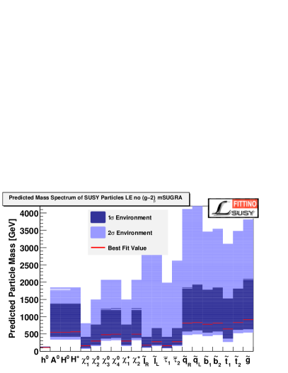
Since the uncertainties of the mSUGRA parameters for the fit without $(g-2)_{\mu}$ in Figure 17 extend to much larger values of the mass parameters, also the maximal values of the sparticle masses allowed at 95 % CL are increasing significantly with respect to the baseline fit or the fit without $\Omega_{\mathrm{CDM}}h^{2}$. This is visible in Figure 18. This result shows again, similar to the result for $a_{\mu}^{\mathrm{exp}}=a_{\mu}^{\mathrm{SM}}$, that $(g-2)_{\mu}$ plays a major role in constraining the allowed mSUGRA sparticle masses to values below 1.6 TeV in the baseline fit.

Table 13: Result of the fit of the mSUGRA model with $\mathrm{sign}(\mu)=+1$ including four additional SM parameters to all measurements listed in Table 1 except $\Omega_{\mathrm{CDM}}h^{2}$ and $(g-2)_{\mu}$. The minimum $\chi^{2}$ value is $19.5$ for 20 degrees of freedom, corresponding to a ${\cal P}$-value of 49.1 %. Due to the very weak remaining constraint on the SUSY parameter space, in this fit a complete coverage of the possible two-dimensional $2\,\sigma$ parameter space can not be ensured within the available statistics. Hence the uncertainties are to be treated as lower boundaries on the uncertainties.

Parameter	Best Fit		Uncertainty
sign$(\mu)$	+1
$\alpha_{s}$	0.1179	$\pm$	0.0021
$1/\alpha_{em}$	127.925	$\pm$	0.015
$m_{Z}$ (GeV)	91.1876	$\pm$	0.0022
$m_{t}$ (GeV)	172.4	$\pm$	1.2
$\tan\,\beta$	7.4		${}_{-4.7}^{+47.3}$
$M_{1/2}$ (GeV)	432.6		${}_{-307.1}^{+4405.6}$
$M_{0}$ (GeV)	64.3		${}_{-62.8}^{+6816.7}$
$A_{0}$ (GeV)	387.8		${}_{-10364.9}^{+6341.4}$

The previous results show that $\Omega_{\mathrm{CDM}}h^{2}$ has a strong role in constraining the size of the uncertainties, but does not affect the best fit result or the shape of the predicted sparticle mass spectrum. On the other hand, $(g-2)_{\mu}$ has a decisive impact on the shape of the allowed parameter regions, the best fit values of the parameters, their uncertainties and hence on the predicted particle spectrum. The prediction of a rich sparticle spectrum in the kinematic range accessible by the LHC however remains stable for all explored fits including or excluding either $\Omega_{\mathrm{CDM}}h^{2}$ or $(g-2)_{\mu}$, which is a very encouraging result for the discovery potential of LHC. The question remains whether there are other observables among those shown in Table 1 which constrain the mSUGRA parameter space. This is addressed by removing both $\Omega_{\mathrm{CDM}}h^{2}$ and $(g-2)_{\mu}$ from the fit and looking for remaining constraints. The result of this fit with $\mathrm{sign}(\mu)=+1$ is shown in Table 13. The results show that the uncertainties increase strongly with respect to the baseline fit as well as with respect to the fits without either $\Omega_{\mathrm{CDM}}h^{2}$ or $(g-2)_{\mu}$. This shows both the complementarity of the $\Omega_{\mathrm{CDM}}h^{2}$ and $(g-2)_{\mu}$ constraints, respectively, and the lack of other strongly constraining observables in Table 1. Since no significant constraints on low-energy SUSY can be placed anymore without these observables, the corresponding fit with $\mathrm{sign}(\mu)=-1$ is omitted.

Figure 19: mSUGRA parameter regions compatible with the collider precision observables from Table 1 and with the requirement of a neutral LSP, but without any requirement on $\Omega_{\mathrm{CDM}}h^{2}$ and $(g-2)_{\mu}$, overlaid with the allowed parameter regions using only no $\Omega_{\mathrm{CDM}}h^{2}$ or no $(g-2)_{\mu}$.

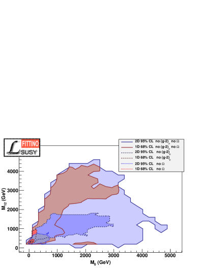
A comparison of the size of the allowed parameter space in the $M_{0}$ and $M_{1/2}$ projections, for the fits without $\Omega_{\mathrm{CDM}}h^{2}$, $(g-2)_{\mu}$ and without both is shown in Figure 19. For the fit without both observables the Markov Chains does not completely explore the two-dimensional $2\,\sigma$ uncertainty space, hence the uncertainty region is to be interpreted as a lower bound on the uncertainties. This could be remedied by using significantly larger statistics in the Markov Chains. For the result shown here this is not done, since the results show clearly that SUSY within the reach of the LHC or the ILC is not ensured without using $\Omega_{\mathrm{CDM}}h^{2}$ and $(g-2)_{\mu}$.

Figure 20: SUSY mass spectrum as predicted by mSUGRA parameter fit to low energy measurements except $(g-2)_{\mu}$ and $\Omega_{\mathrm{CDM}}h^{2}$ with sign$(\mu)$ fixed to $+1$.

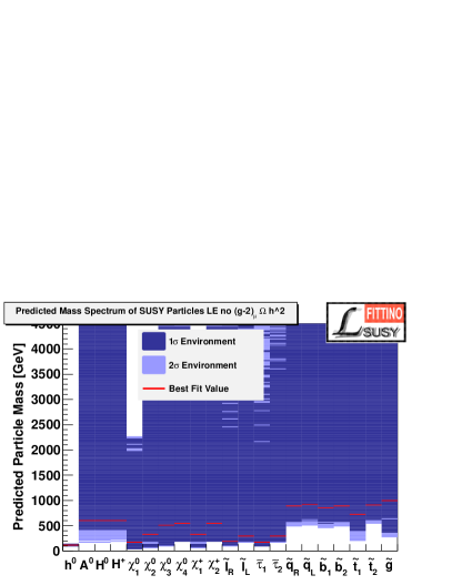
A part of the allowed sparticle mass spectrum is shown in Figure 20. The $1\,\sigma$ allowed ranges of all particles apart from the lightest Higgs boson, neutralino and chargino extend well beyond a mass of $4\,\mathrm{TeV}$. Hence no discovery at LHC or ILC can be predicted apart from the SM-like lightest SUSY Higgs boson, which is difficult to be distinguished from the SM Higgs boson at the LHC AguilarSaavedra:2001rg . The allowed mass range of the lightest Higgs boson is $m_{h}=114.0^{+14}_{-3}\,\mathrm{GeV}$, showing that the precision data still has a tendency to push the Higgs mass towards the lowest values allowed by the direct searches. At the same time, the push is not strong enough to exclude that the light Higgs boson mass is close to the theoretically allowed upper limit at around $m_{h}^{\mathrm{theo}}<135\,\mathrm{GeV}$ in this scenario.

No detailed effect of other observables is tested due to the failure of the remaining observables to constrain the mSUGRA parameter space to the region accessible with the next generation of collider experiments. However, this does not mean that the precision observables or the flavour physics data will not have a decisive role in helping to understand SUSY once sparticles are discovered. The reasons for the strong impact of the precision data are demonstrated in Section 4.3. If a Higgs boson is discovered, the precision of its mass measurement will be much better than the precision of $\sigma_{m_{h}}\approx\pm 3\,\mathrm{GeV}$ obtained from the low-energy, cosmological and precision data. Therefore a further improvement on the uncertainties of the precision observables would be beneficial for an ultimate cross-check of the collider data below and above the electro-weak scale.

In addition, Figure 20 shows a very clear impact of the precision and flavour physics observables and especially of the Higgs searches at LEP in form of an implicit lower bound on the sparticle masses above or around the current direct search limits (e. g. Heister:2003zk ; Abazov:2009zi ; Aaltonen:2009fm ; Heister:2001nk ). The lightest neutralino mass is expected above 45 GeV, the lightest chargino mass above 100 GeV, and the $\tilde{\tau}_{1}$ mass above 110 GeV. A small region with a chargino NLSP is allowed at the $2\,\sigma$ level, with most points featuring a $\tilde{\tau}_{1}$ NLSP.

4.1.3 Fits of the GMSB Model

The mSUGRA scenario studied so far has the strong advantage that it solves a very large amount of experimental and theoretical challenges of the SM. In addition, it is very well studied at colliders, making it an ideal testing ground. Therefore it is the main SUSY scenario studied in this paper. However, it is not the only way how SUSY can be broken at the expected Grand Unified Theory scale of around $\Lambda_{\mathrm{GUT}}\approx 10^{16}\,\mathrm{GeV}$. As an example of a different SUSY breaking mechanism, Gauge Mediated Supersymmetry Breaking (GMSB) Dine:1994vc is explored. It has the disadvantage that it includes a very light gravitino in the range of $m_{\tilde{G}}\approx{\cal O}(1-10\,\mathrm{MeV})$ as LSP, which leads to hot dark matter. This is difficult to be reconciled with structure formation in the Universe Pierpaoli:1997im ; Staub:2009ww . Therefore, $\Omega_{\mathrm{CDM}}h^{2}$ is not included in the analysis.

Table 14: Result of the fit of the GMSB model with different values of sign$(\mu)$ and $N_{5}$ including four additional SM parameters to all measurements listed in Table 1 except $\Omega_{\mathrm{CDM}}h^{2}$. The minimum $\chi^{2}$ value is $19.30$ for 21 degrees of freedom, corresponding to a ${\cal P}$-value of 56.5 %. The uncertainties correspond to the entry for $\mathrm{sign}(\mu)=+1$ and $N_{5}=1$.

Parameter	Best Fit	Best Fit	Best Fit	Best Fit	Best Fit		Uncertainty for
							$N_{5}=1,\mathrm{sign}(\mu)=+1$
sign$(\mu)$	+1	-1	+1	+1	+1
$N_{5}$	1	1	2	3	4
$\tan\,\beta$	19.2	19.4	17.9	18.3	18.5		${}_{-6.7}^{+15.3}$
$\Lambda$ (GeV)	87050	307629	53284	40080	32643		${}_{-17151}^{+31970}$
$M_{\mathrm{mess}}$ (GeV)	431752	334662	688567	$1.038\times 10^{6}$	539328		${}_{-352952}^{+1.74\times 10^{6}}$
$C_{\mathrm{grav}}$	411.4	446.1	885.5	460.1	3368.1		${}_{-411.3}^{+10042.5}$
$\chi^{2}_{\mathrm{min}}$	19.3	31.0	19.4	19.5	19.5

In GMSB, there are four continuous variables: $\tan\beta=v_{2}/v_{1}$ is the ratio of the Higgs vacuum expectation values, $\Lambda$ is universal mass scale of SUSY particles at the GUT scale, $M_{\mathrm{mess}}$ denotes the mass scale of the messenger gauge particles between the SUSY breaking sector and the visible sector, and $C_{\mathrm{grav}}$ is the scale of the gravitino coupling. In addition, there are two discrete parameters, namely $\mathrm{sign}(\mu)$ and the number of messenger fields $N_{5}$. As before, separate fits are performed for different values of the discrete parameters. A selection of the results is shown in Table 14. It can be seen that there is a similar sensitivity to $\mathrm{sign}(\mu)$ through the positive value of $a_{\mu}^{\mathrm{exp}}-a_{\mu}^{\mathrm{SM}}$. There is, however, no sensitivity to $N_{5}$, since all performed fits with $N_{5}=1,2,3,4$ achieve the same value of $\chi^{2}_{\mathrm{min}}=19.5$, corresponding to a ${\cal P}$-value of 56.5 %. It can be seen that no sensitive limit can be placed on $M_{\mathrm{mess}}$ and $C_{\mathrm{grav}}$, while $\tan\beta$ and $\Lambda$ can be constrained. Since the prediction for $\tan\beta$ and $\Lambda$ is stable for different areas in $M_{\mathrm{mess}}$ and $C_{\mathrm{grav}}$, the remaining large uncertainty does not affect the constrained regions for $\tan\beta$ and $\Lambda$ given the existing measurements. This shows an interesting complementarity to the expected LHC measurements, where constraints cannot be set on $\tan\beta$ and $C_{\mathrm{grav}}$ or $M_{\mathrm{mess}}$ alone, but on $C_{\mathrm{grav}}\times M_{\mathrm{mess}}$ Culbertson:2000am through the measurement of sparticle masses and gaugino lifetimes.

Figure 21: Pull for the low energy observables used in the GMSB parameter fit with $N_{5}=1$ and sign$(\mu)=+1$, using the observables from Table 1 and the best fit point from Table 14.

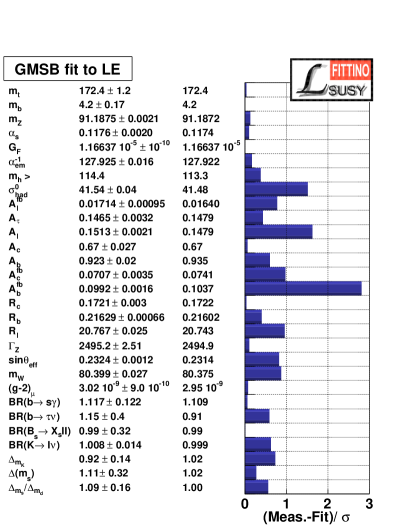
The pull of the individual variables with respect to the best fit result of the fit with $\mathrm{sign}(\mu)=+1$ and $N_{5}=1$ is shown in Figure 21. The obtained pattern is very similar to the pattern for the mSUGRA scenario, which again confirms that the tension of the SM with the electro-weak precision observables cannot be remedied by Supersymmetry, apart from moving the Higgs boson mass close to or above the experimental limit. The prediction of GMSB is $m_{h}=(113.5\pm 2)\,\mathrm{GeV}$, very similar to mSUGRA.

Figure 22: GMSB parameter regions with sign$(\mu)=+1$ and different values of $N_{5}$ compatible with the existing data from Table 1 except $\Omega_{\mathrm{CDM}}h^{2}$.

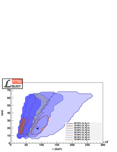
The allowed parameter range in $\tan\beta$ and $\Lambda$ is shown in Figure 22 for different values of $N_{5}$. It is interesting to observe that, as already visible in Table 14, the predictions and hence $\chi^{2}_{\mathrm{min}}$ remains unchanged for different values of $N_{5}$. There are different preferred parameter regions in $\Lambda$, leaving $\Lambda\times N_{5}$ approximately unchanged. Intermediate values of $\tan\beta$ are preferred, but neither large nor high values can be excluded at the $2\,\sigma$ level.

Figure 23: SUSY mass spectrum as predicted by GMSB parameter fit to low energy measurements except $\Omega_{\mathrm{CDM}}h^{2}$ with $N_{5}$ fixed to 1 and sign$(\mu)=+1$.

Figure 24: SUSY mass spectrum as predicted by GMSB parameter fit to low energy measurements except $\Omega_{\mathrm{CDM}}h^{2}$ with $N_{5}$ fixed to 2 and sign$(\mu)=+1$.

Figure 25: SUSY mass spectrum as predicted by GMSB parameter fit to low energy measurements except $\Omega_{\mathrm{CDM}}h^{2}$ with $N_{5}$ fixed to 3 and sign$(\mu)=+1$.

Figure 26: SUSY mass spectrum as predicted by GMSB parameter fit to low energy measurements except $\Omega_{\mathrm{CDM}}h^{2}$ with $N_{5}$ fixed to 4 and sign$(\mu)=+1$.

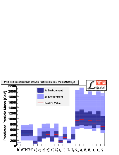
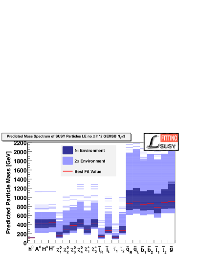
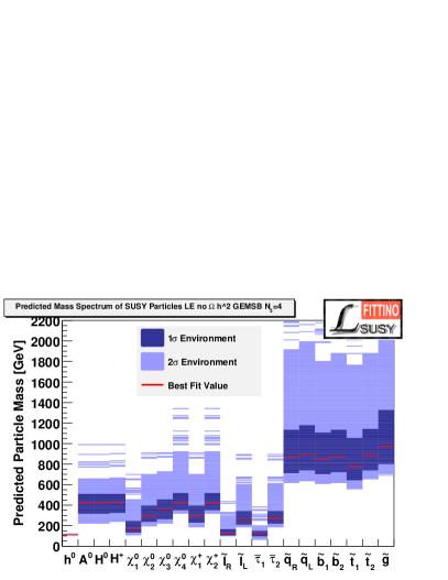
The predicted sparticle spectrum is also insensitive to $N_{5}$ itself, as shown in Figures 23 to 26, where an almost perfect agreement between the spectra for different values of $N_{5}$ is shown. Generally the expected spectrum looks similar to the expected mSUGRA spectrum. This is a strong hint that given the existing measurements, Supersymmetry generally provides for the prediction of a rich observable particle spectrum at the LHC, independent of the SUSY breaking mechanism. In GMSB, there is a tendency towards higher values of the squark and gluino masses with respect to mSUGRA, but the difference in the predictions is not decisive enough to base a distinction between the scenarios on the mass hierarchies for scenarios with similar visible parts of the decay chains in GMSB and mSUGRA.

4.1.4 Conclusions for SUSY Scenarios at Colliders

The results show that Supersymmetry, broken at the GUT scale, offers several possibilities to fit the existing precision data. In the mSUGRA breaking scenario, all parameters can be constrained and the existing data from cosmological, low-energy, flavour physics and precision collider sources clearly prefer parameter ranges which are accessible at the next generation of collider experiments. It is shown that as expected $\Omega_{\mathrm{CDM}}h^{2}$ and $(g-2)_{\mu}$ provide for the most sensitive constraints among the available measurements. Even if individual, very sensitive, variables are removed, or if deviations between data and the SM prediction are assigned to unknown systematic uncertainties, a clear constraint in the accessible mass regions remains. Only voluntarily removing both $\Omega_{\mathrm{CDM}}h^{2}$ and $(g-2)_{\mu}$ simultaneously from the list of observables used in the fit, removes the experimental constraint to the parameter region accessible at the LHC.

The best fit parameter spectrum and the uncertainties from present data clearly prefers a SUSY scenario with a rich phenomenology both at the LHC and the ILC. At the $1\,\sigma$ level, all Higgs bosons, gauginos (apart from the gluino) and all sleptons are expected below $m\leq 600\,\mathrm{GeV}$. The squarks and gluinos are expected below $m\leq 900\,\mathrm{GeV}$. While this provides for relatively early discovery at the LHC, the rich expected spectrum with many concurrent production and decay modes will contribute to a challenging reconstruction of the LHC observables sensitive to SUSY masses and branching fractions. In particular, a very small mass difference between the neutralino LSP and the NLSP, which is the $\tilde{\tau}_{1}$ of $m_{\mathrm{NLSP}}-m_{\mathrm{LSP}}<22\,\mathrm{GeV}$ at the 95 % CL level leads to dominating decays of the gauginos into final states with $\tau$ leptons. However, the exact branching fractions cannot be predicted with strong precision.

4.2 Expected LHC Measurements

Based on the results of the previous section, we now investigate the prospects for the determination of SUSY parameters from future LHC measurements. Within the mSUGRA model, the preferred parameters from existing LE measurements and constraints clearly point towards rather light sparticle masses. In order to be consistent with the measured dark matter relic density, co-annihilation of the LSP and the NLSP has to contribute to the dark matter annihilation process. For this process to be efficient, the mass difference between NLSP and LSP has to be rather small. For the best fit point, within mSUGRA, the difference $m(\tilde{\tau}_{1})-m(\tilde{\chi}^{0}_{1})$ is only 8 GeV, and the difference $m(\tilde{e}_{R})-m(\tilde{\chi}^{0}_{1})$ is 22 GeV. No detailed experimental studies for LHC prospects are available for this specific parameter point. However, detailed studies exist for the SPS1a parameter point with parameters $\tan\beta=10$, $A_{0}=-100$ GeV, $M_{1/2}=250$ GeV, $M_{0}=100$ GeV, sign$(\mu)=+1$ Allanach:2002nj . These parameters taken at face value lead to a significantly larger dark matter relic density due to mass differences $m(\tilde{\tau}_{1})-m(\tilde{\chi}^{0}_{1})=37$ GeV and $m(\tilde{e}_{R})-m(\tilde{\chi}^{0}_{1})=47$ GeV. Apart from this difference, the collider phenomenology of SPS1a is very similar to that of the best fit point. The smaller mass differences lead to softer spectra for the final state leptons, which is a small caveat to be kept in mind in the following analysis and should serve to trigger more optimisation of soft lepton identification within the LHC experiments. We assume in the following as a plausible scenario that SUSY is realised with electro-weak scale parameters derived from the high-scale SPS1a parameters and will be discovered by the LHC experiments. As input measurements we use the observables specified in Section 2.2 for three different integrated luminosities. If taken at face value, the lightest Higgs boson mass in SPS1a calculated with SPheno is 109 GeV, slightly below the LEP exclusion. Given the theoretical uncertainty as well as the strong dependence of $m_{h}$ on the top quark mass we do not consider this as an inevitable constraint. Technically, we set the LEP Higgs mass limit slightly below 109 GeV for the luminosity scenarios where no Higgs boson has been found yet at the LHC and we assume that a 109 GeV Higgs boson could be discovered at the LHC with similar sensitivity as for 115 GeV.

4.2.1 mSUGRA Fit with fixed sign$(\mu)$

Figure 27: Results of the Toy Fits to the expected LHC “measurements” from Table 2 for different integrated luminosities. The upper plots show the expected distribution of best fit points, exhibiting the strong increase in precision for ${\cal L}^{\mathrm{int}}\geq 10\,\mathrm{fb}^{-1}$. The lower row of plots shows the $\chi^{2}$ distributions for the Toy Fits with integrated luminosities of 1 fb^-1 and 300 fb^-1, showing very good agreement with the expected $\chi^{2}$ distributions for the respective degrees of freedom.

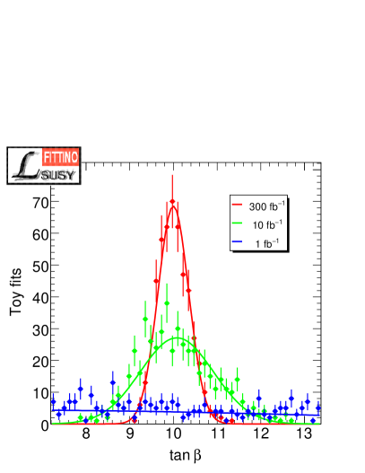
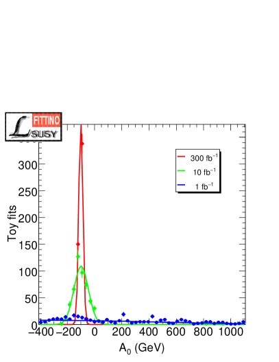
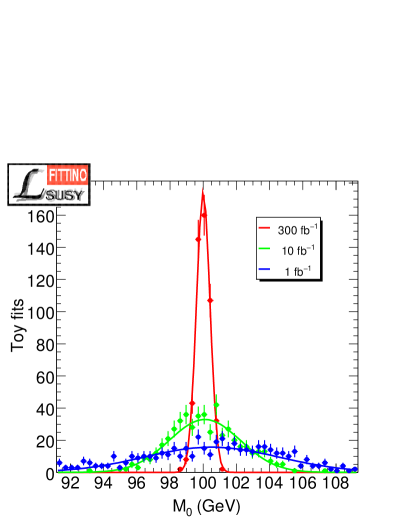
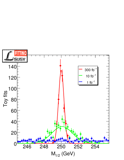
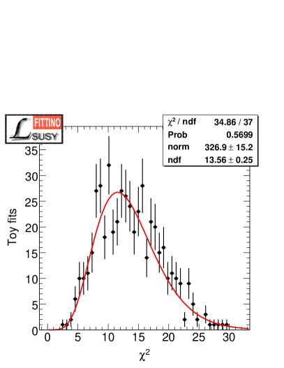
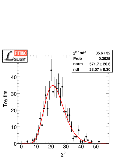
The good agreement in collider phenomenology between SPS1a and the mSUGRA best fit point offers the possibility to use the wealth of Monte Carlo studies performed for this benchmark point to attempt a projection of the SUSY model discrimination power and parameter constraints to the LHC era. This is done by performing fits to Toy data which have been obtained by smearing the observable values according to a Gaussian around the nominal SPS1a values as explained in Section 3. In the top four plots in Figure 27 the distributions for the fitted parameters from these Toy Fits are shown assuming $\mu>0$ for integrated luminosities of 1 fb^-1, 10 fb^-1 and 300 fb^-1. The fitted central values and their uncertainties are obtained from a Gaussian fit to the parameter distributions. The corresponding values are listed in Table 15, 16 and 17. The two bottom plots of Figure 27 display, as examples, the $\chi^{2}$ distributions from the Toy Fits for the smallest and largest considered luminosity. The fact that the $\chi^{2}$ distributions are in very good agreement with the expectations for the respective degrees of freedom provides confidence that the $\chi^{2}$ minimisation algorithm works reliably.

Already with 1 fb^-1 of LHC data it is possible to constrain the scalar mass parameter $M_{0}$ and the gaugino mass parameter $M_{1/2}$ to the level of a few percent due to the already relatively precise measurements of the endpoints of the $\ell q$ and the $\ell\ell q$ invariant mass spectra. For the determination of $M_{1/2}$ also the $m_{T2}$ measurement in events with $\tilde{q}_{R}\to q\tilde{\chi}_{1}^{0}$ decays is important. $\tan\beta$ and $A_{0}$ are more difficult to determinee. For $\tan\beta$, approximately 40 % precision and for $A_{0}$ only an order of magnitude estimate is obtained. With 1 fb^-1 the best constraints on these parameters come from measurements involving third generation particles, in particular from $m_{tb}^{w}$.

Table 15: Result of the fit of the mSUGRA model to the expected LHC observables for 1 fb^-1.

Parameter	Best Fit		Uncertainty
sign$(\mu)$	$+$1
$\tan\,\beta$	9.1	$\pm$	3.7
$A_{0}$ (GeV)	$-$131.8	$\pm$	742.1
$M_{0}$ (GeV)	100.2	$\pm$	4.2
$M_{1/2}$ (GeV)	249.7	$\pm$	6.7

The increased precision on $M_{0}$ for an integrated luminosity of 10 fb^-1 mainly comes from more precise measurements of the endpoints of the $\ell q$ spectra. For $M_{1/2}$ also new sensitive measurements become available with a larger data sample, in particular $m_{\tilde{g}}-m_{\tilde{\chi}_{1}^{0}}$. The measurement of $m_{tb}^{w}$ still remains important to constrain $\tan\beta$ and $A_{0}$. In addition $m_{\ell\ell}^{\mathrm{max}}$ from $\tilde{\chi}_{4}^{0}$ decays provides valuable additional information on $\tan\beta$ and $A_{0}$ at 10 fb^-1. For $\tan\beta$ also the ratio of branching fractions (2) starts to contribute.

Table 16: Result of the fit of the mSUGRA model to the expected LHC observables for 10 fb^-1.

Parameter	Best Fit		Uncertainty
sign$(\mu)$	$+$1
$\tan\,\beta$	10.08	$\pm$	0.84
$A_{0}$ (GeV)	$-$98.0	$\pm$	52.9
$M_{0}$ (GeV)	100.1	$\pm$	2.1
$M_{1/2}$ (GeV)	250.1	$\pm$	1.2

With 300 fb^-1 of LHC data it will finally be possible to constrain $M_{0}$ and $M_{1/2}$ down to (a few) permille level. The driving factor is an increased precision on $m_{\ell q}^{\mathrm{high}}$, $m_{\ell q}^{\mathrm{low}}$ and – in case of $M_{1/2}$ – also on $m_{\ell\ell q}^{\mathrm{max}}$. Similarly the improvement on $A_{0}$ can be traced back to better measurements of those observables which already provide the best constraints for 10 fb^-1, namely $m_{\ell\ell}^{\mathrm{max}}$ from $\tilde{\chi}_{4}^{0}$ decays and $m_{tb}^{w}$. $\tan\beta$ at 300 fb^-1 is mainly controlled by measurements of quantity (2) and the lightest Higgs mass $m_{h}$. For $\tan\beta$ ($A_{0}$) a relative precision of approximately 4 % (11 %) is finally achieved from the given list of observables.

Table 17: Result of the fit of the mSUGRA model to the expected LHC observables for 300 fb^-1.

Parameter	Best Fit		Uncertainty
sign$(\mu)$	$+$1
$\tan\,\beta$	9.98	$\pm$	0.35
$A_{0}$ (GeV)	$-$100.2	$\pm$	11.1
$M_{0}$ (GeV)	100.0	$\pm$	0.39
$M_{1/2}$ (GeV)	250.0	$\pm$	0.30

Concerning the most constraining observables mentioned above it should be noted that they might be very sensitive to small changes of the input measurements. Therefore they ought to be taken with some care and should not be generalised without further cross-checks.

4.2.2 Determination of sign$(\mu)$

Figure 28: $\chi^{2}$ correlations for mSUGRA fits with $\mu>0$ and $\mu<0$ to the same Toy data set (left/middle/right for an integrated LHC luminosity of 1 fb^-1/10 fb^-1/300 fb^-1).

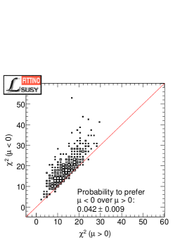
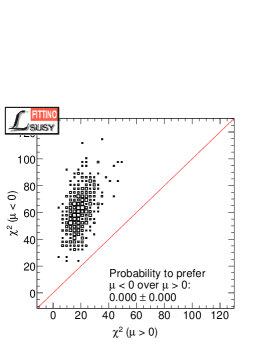
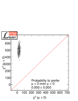
For the LHC fit results described above, we have not yet discussed how to find the correct sign of $\mu$. Using the technique described in Section 3.2, we also checked how well the sign of $\mu$ can be determined from LHC data. This is done by performing Toy Fits for each sign of $\mu$ to the identical set of Toy data. Figure 28 shows the $\chi^{2}$ correlations obtained from such fits. If we choose the value for sign of $\mu$ which yields the best $\chi^{2}$ for a given set of LHC measurements we can estimate the probability to make the wrong choice by counting the number of Toy Fits below the red bisecting line in Figure 28 and normalise it to the total number of Toy Fits. The corresponding numbers can be read off the plots. Already with 1 fb^-1 there is a good chance to extract sign$(\mu)$ correctly. The probability for a wrong choice is less than 5 %. Based on 10 fb^-1 or more of LHC data, sign$(\mu)$ can be determined with negligible error probability.

4.2.3 First Investigation of Chain Ambiguities

Figure 29: $\chi^{2}$ correlations obtained from fits to the same Toy data set for two different interpretations of $m_{\ell\ell}^{\text{max}}$.

Figure 30: Parameter distributions (for 10 fb^-1) of the mSUGRA model of two different interpretations of the data, fitted to the same Toy data set. The parameter distributions assuming the correct endpoint assignment is shown in blue, those using the wrong interpretation is indicated in red and the distribution which is obtained if always the interpretation with the lowest minimal $\chi^{2}$ is chosen is displayed in black.

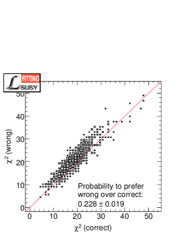
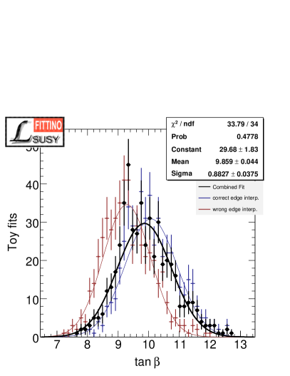
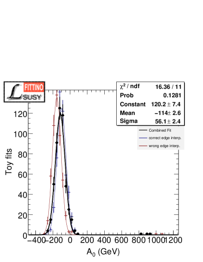
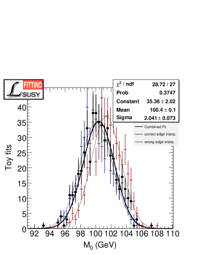
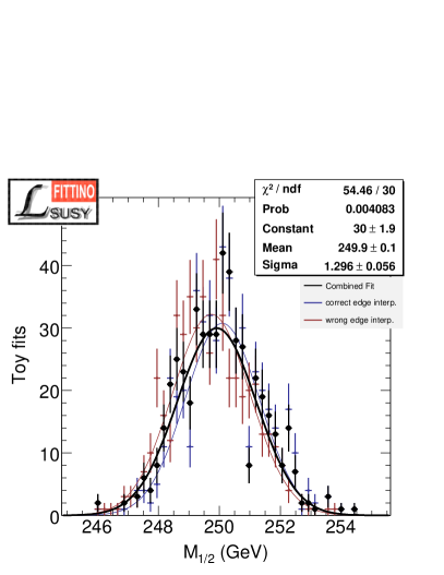
All the above LHC fit results are based on the idealised assumption that one knows the contributing decay chain for a given mass spectrum. In reality this is, of course, not the case. Therefore there are in general various possible decays which can contribute to a specific mass spectrum. In the context of this study we do not yet address this problem systematically. A fully realistic analysis, taking the full combinatorics for such chain ambiguities into account, can be performed when data are present. Here we constrain ourselves to the case where we check the impact of misinterpreting a single observable to test the methodology. To accomplish this we perform fits to the same Toy data set for each possible interpretation of a mass spectrum. As an example we allow for two different interpretations of one particular di-lepton endpoint as either (correct) $m_{\ell\ell}^{\text{max}}(m_{\tilde{\chi}_{1}^{0}},m_{\tilde{\chi}_{4}^{0}},m_{\tilde{\ell}_{L}})$ or (wrong) $m_{\ell\ell}^{\text{max}}(m_{\tilde{\chi}_{1}^{0}},m_{\tilde{\chi}_{4}^{0}},m_{\tilde{\ell}_{R}})$ for the case of 10 fb^-1 of integrated luminosity.

Figure 29 shows the $\chi^{2}$ correlations obtained from fits to the same Toy data set for these two different interpretations of $m_{\ell\ell}^{\text{max}}$. If one always chooses the interpretation which yields the smallest minimal $\chi^{2}$ the probability to make a wrong decision is approximately 23 %. Figure 30 shows the mSUGRA parameter distributions from Toy Fits assuming the correct endpoint assignment (blue), the wrong interpretation (red) and the distribution which is obtained if the one with the lowest minimal $\chi^{2}$ is always chosen (black). It is apparent that this chain ambiguity has some impact on the reconstructed parameters leading to a bias on the mean and to systematically larger values for the uncertainties on the parameters, but these effects are rather small compared to the uncertainty on the parameters. While this observation certainly cannot be generalised to arbitrary ambiguities in the decay chains, the principal method can always be applied. Depending on the result of the $\chi^{2}$ comparison, the ambiguity can be either translated into increased parameter errors or certain hypotheses can be discarded if they yield significantly worse $\chi^{2}$.

4.3 Role of Low Energy Observables in the LHC Era

Now we address the question to which extent low energy measurements still contribute to the determination of SUSY parameters once LHC results become available. We perform this study for two different SUSY models, namely mSUGRA and MSSM18. The input observables for these analyses comprise all the low energy observables listed in Table 1 in addition to the LHC observables of Table 2. To ensure a consistent set of “measurements” for these analyses, nominal SPS1a values are used for the low energy observables instead of the actually measured values.

Figure 31: Discrimination power of the expected low-energy and LHC results from Table 1 and 2 for ${\cal L}^{\mathrm{int}}=1\,\mathrm{fb}^{-1}$ (left) and ${\cal L}^{\mathrm{int}}=10\,\mathrm{fb}^{-1}$ in a 2-dimensional plot of the minimal $\chi^{2}$ values of simultaneous Toy Fits of two different models ($\mathrm{sign}(\mu)=+1$ and $\mathrm{sign}(\mu)=-1$). In comparison with Figure 28 a clear increase in separation power for ${\cal L}^{\mathrm{int}}=1\,\mathrm{fb}^{-1}$ is observed.

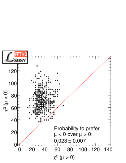
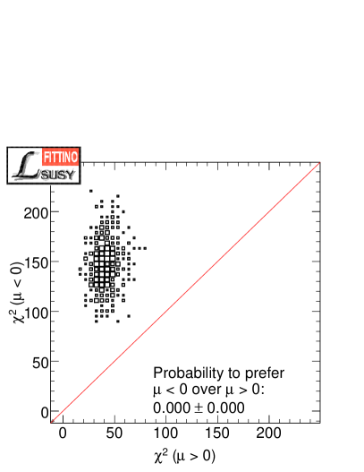
4.3.1 mSUGRA Fit

Figure 32: Results of the Toy Fits to the low-energy measurements and the expected LHC results from Table 1 and 2 for different integrated luminosities. The upper plots shows the expected distribution of best fit points, exhibiting the strong increase in precision for ${\cal L}^{\mathrm{int}}\geq 10\,\mathrm{fb}^{-1}$. The lower row of plots shows the $\chi^{2}$ distributions of the Toy Fits with integrated luminosities of 1 fb^-1 and 300 fb^-1, showing very good agreement with the expected degrees of freedom. In comparison with Figure 27, a clear increase in precision is observed, especially for ${\cal L}^{\mathrm{int}}=1\,\mathrm{fb}^{-1}$ and for the parameters $\tan\beta$ and $M_{0}$.

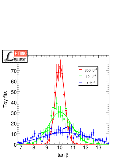
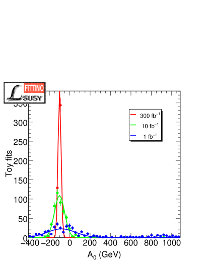
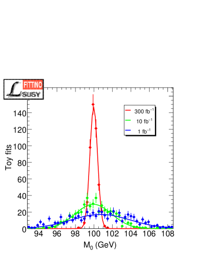
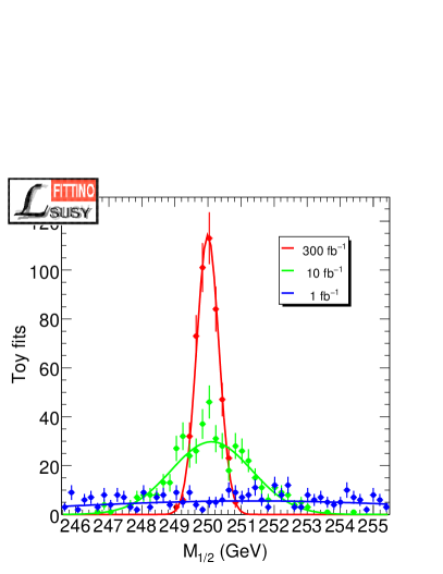
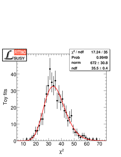
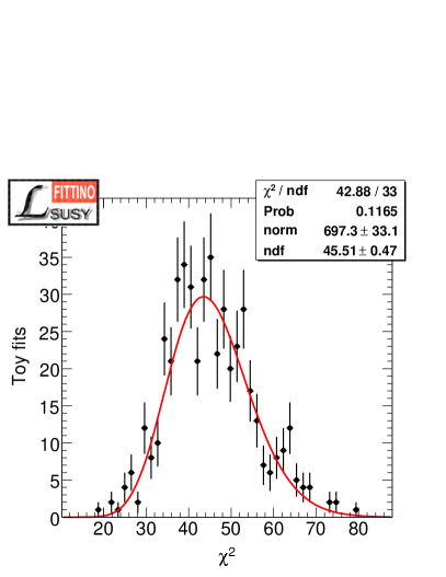
The fit results of the mSUGRA Toy Fits using low energy and LHC observables for the three different luminosities are shown in Figure 32. The corresponding fitted mSUGRA parameters and the corresponding correlation coefficients are summarised in Tables 18, 19, 20, 21, 22 and 23. As described in Section 4.2 $\tan\beta$ and $A_{0}$ are rather weakly constrained by LHC measurements alone at low luminosity. For these parameters the addition of low energy measurements clearly improves the situation. At 1 fb^-1, $(g-2)_{\mu}$ is an important additional measurement constraining $\tan\beta$ and $A_{0}$. For $M_{0}$, the cold dark matter relic density $\Omega_{\mathrm{CDM}}h^{2}$ becomes the most sensitive observable followed by $m_{\ell q}^{\mathrm{high}}$, the most important LHC quantity. The precision on $M_{1/2}$ is still dominated by the LHC “measurements” listed in Section 4.2. Nevertheless some improvements are also achieved for this parameter, mainly due to $(g-2)_{\mu}$.

At 10 fb^-1 and above the role of low energy measurements is largely repressed by LHC observables such that the precision on the mSUGRA parameters for increasing luminosity asymptotically approaches the precision obtained from LHC observables alone.

These results can be used to derive the complete SUSY particle mass spectrum assuming the mSUGRA model and the best fitting parameters. Figure 33 shows the mass spectrum for an integrated LHC luminosity of 1 fb^-1 as obtained from low energy and LHC observables. The respective mean and most probable values are indicated in black and red. $1\,\sigma$, $2\,\sigma$ and $3\,\sigma$ uncertainties are indicated by the blue bands. It should be noted that the masses derived in this way are model dependent statements and not direct mass measurements. While the masses of the light Higgs boson, the light gauginos and the sleptons can already be constrained quite well, the masses of the heavy Higgs bosons, the heavy gauginos and the squarks are still quite imprecise. The situation improves significantly if one goes to a luminosity of 10 fb^-1 (see Figure 34). Increasing the luminosity to 300 fb^-1 (Figure 35) again means a clear increase in precision with respect to the 10 fb^-1 result. This means that stringent spectroscopic tests of the mSUGRA model will be possible using the experimentally accessible sparticles and precise mass predictions are feasible for those SUSY particles which cannot be directly probed at the LHC.

In addition to Toy Fits we also perform a Markov Chain analysis. Figure 36 shows the quantity $\Delta\chi^{2}=-2\ln(\mathcal{L})+2\ln(\mathcal{L}_{\mathrm{max}})$ for all possible mSUGRA parameter pairs for the three considered LHC luminosities of 1 fb^-1/10 fb^-1/300 fb^-1 (left/middle/right). $\mathcal{L}$ is the two-dimensional profile likelihood and $\mathcal{L}_{\mathrm{max}}$ the global maximum of the likelihood. The black dotted contours represent $\Delta\chi^{2}=1$ contours. The results are in good agreement with those obtained from the Toy Fits and nicely show the partly strong correlation between the parameters which is also reflected in Tables 19, 21 and 23.

For illustrative purposes Figure 37 shows the outcome of the same Markov Chain for the parameter pair $A_{0}$-$\tan\beta$ using Bayesian statistics. The lines again indicate $\Delta\chi^{2}=-2\ln(\mathcal{L})+2\ln(\mathcal{L}_{\mathrm{max}})$ contours but this time $\mathcal{L}$ denotes the marginalised posterior probability (using a flat prior probability). Compared to the results derived from the profile likelihood the contour lines are more jagged for the same Markov Chain length. Apart from these fluctuations good agreement between the results derived from the marginalised posterior probability and those from the profile likelihood (shown in Figure 36) is found.

Table 18: Result of the fit of the mSUGRA model to low energy and LHC observables for 1 fb^-1.

Parameter	Best Fit		Uncertainty
sign$(\mu)$	$+$1
$\tan\,\beta$	10.2	$\pm$	2.3
$A_{0}$ (GeV)	$-$76.3	$\pm$	184
$M_{0}$ (GeV)	100.6	$\pm$	3.4
$M_{1/2}$ (GeV)	250.2	$\pm$	5.3

Figure 33: SUSY mass spectrum consistent with the existing low-energy measurements from Table 1 and the expected LHC measurements from Table 2 at ${\cal L}^{\mathrm{int}}=1\,\mathrm{fb}^{-1}$ for the mSUGRA model. The uncertainty ranges represent model dependent uncertainties of the sparticle masses and not direct mass measurements. This is especially visible for the heavy Higgs states $A,H$ and $H^{\pm}$, for which no direct measurement is expected in the SPS1a scenario.

Table 19: Correlation coefficients for the fitted parameters of the mSUGRA model to the expected low energy and LHC observables for 1 fb^-1.

	$\tan\,\beta$	$A_{0}$	$M_{0}$	$M_{1/2}$
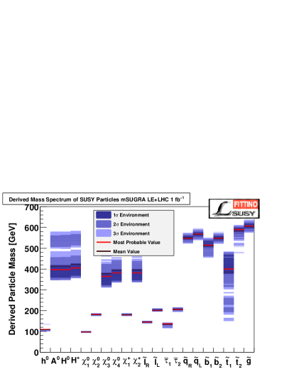
$\tan\,\beta$	1.000	0.534	$-$0.405	0.793
$A_{0}$	0.534	1.000	$-$0.184	0.493
$M_{0}$	$-$0.405	$-$0.184	1.000	$-$0.077
$M_{1/2}$	0.793	0.493	$-$0.077	1.000

Table 20: Result of the fit of the mSUGRA model to low energy and LHC observables for 10 fb^-1.

Parameter	Best Fit		Uncertainty
sign$(\mu)$	$+$1
$\tan\,\beta$	10.0	$\pm$	0.79
$A_{0}$ (GeV)	$-$99.1	$\pm$	48.3
$M_{0}$ (GeV)	100.0	$\pm$	1.9
$M_{1/2}$ (GeV)	250.1	$\pm$	1.1

Figure 34: SUSY mass spectrum consistent with the existing low-energy measurements from Table 1 and the expected LHC measurements from Table 2 at ${\cal L}^{\mathrm{int}}=10\,\mathrm{fb}^{-1}$ for the mSUGRA model. The uncertainty ranges represent model dependent uncertainties of the sparticle masses and not direct mass measurements. With respect to Figure 33, a clear increase in precision is observed.

Table 21: Correlation coefficients for the fitted parameters of the mSUGRA model to the expected low energy and LHC observables for 10 fb^-1.

	$\tan\,\beta$	$A_{0}$	$M_{0}$	$M_{1/2}$
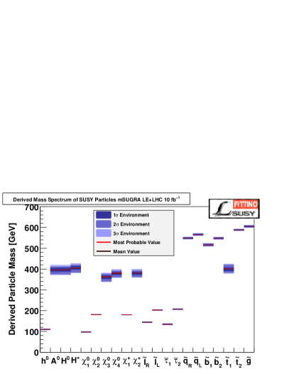
$\tan\,\beta$	1.000	0.805	$-$0.328	0.415
$A_{0}$	0.805	1.000	$-$0.483	0.548
$M_{0}$	$-$0.328	$-$0.483	1.000	0.241
$M_{1/2}$	0.415	0.548	0.241	1.000

Table 22: Result of the fit of the mSUGRA model to low energy and LHC observables for 300 fb^-1.

Parameter	Best Fit		Uncertainty
sign$(\mu)$	$+$1
$\tan\,\beta$	10.00	$\pm$	0.36
$A_{0}$ (GeV)	$-$99.1	$\pm$	12.0
$M_{0}$ (GeV)	100.00	$\pm$	0.39
$M_{1/2}$ (GeV)	250.01	$\pm$	0.33

Figure 35: SUSY mass spectrum consistent with the existing low-energy measurements from Table 1 and the expected LHC measurements from Table 2 at ${\cal L}^{\mathrm{int}}=300\,\mathrm{fb}^{-1}$ for the mSUGRA model. The uncertainty ranges represent model dependent uncertainties of the sparticle masses and not direct mass measurements. With respect to Figure 34, again a clear increase in precision is observed.

Table 23: Correlation coefficients for the fitted parameters of the mSUGRA model to the expected low energy and LHC observables for 300 fb^-1.

	$\tan\,\beta$	$A_{0}$	$M_{0}$	$M_{1/2}$
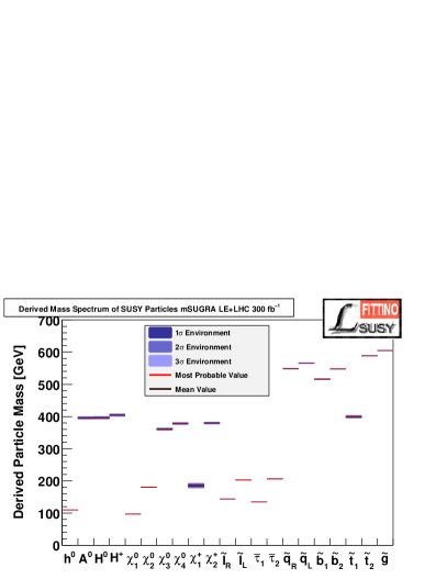
$\tan\,\beta$	1.000	0.356	0.178	0.134
$A_{0}$	0.356	1.000	$-$0.266	0.673
$M_{0}$	0.178	$-$0.266	1.000	0.391
$M_{1/2}$	0.134	0.673	0.391	1.000

Figure 36: $\Delta\chi^{2}=-2\ln(\mathcal{L})+2\ln(\mathcal{L}_{\mathrm{max}})$ contours from Markov Chain for the mSUGRA model using observables from Tables 1 and 2. $\mathcal{L}$ is the two-dimensional profile likelihood and $\mathcal{L}_{\mathrm{max}}$ the global maximum of the likelihood. The black dotted contours represent $\Delta\chi^{2}=1$ contours. The plots are for integrated LHC luminosities of 1 fb^-1/10 fb^-1/300 fb^-1 (left/middle/right).

Figure 37: For comparison with Figure 36, the outcome of the same Markov chain for the parameter pair $A_{0}$-$\tan\beta$ is shown using Bayesian statistics. The lines indicate $\Delta\chi^{2}=-2\ln(\mathcal{L})+2\ln(\mathcal{L}_{\mathrm{max}})$ contours with $\mathcal{L}$ being the marginalised posterior probability (using a flat prior probability). The black dotted contours represent $\Delta\chi^{2}=1$ contours.

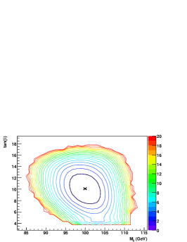
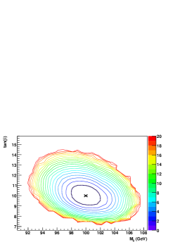
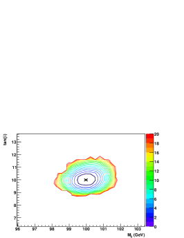
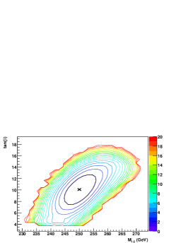
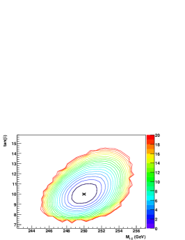
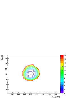
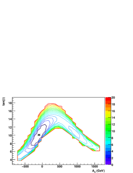
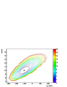
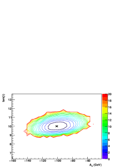
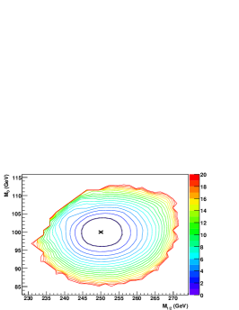
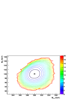
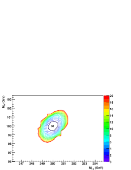
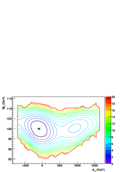
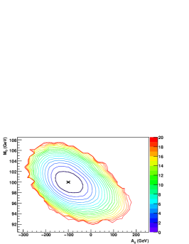
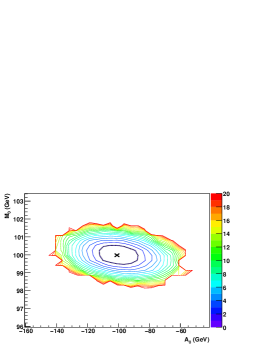
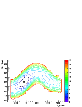
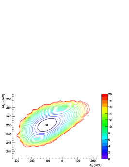
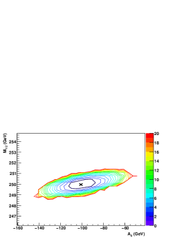
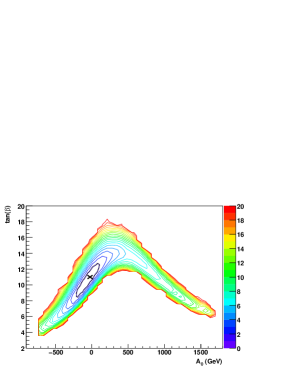
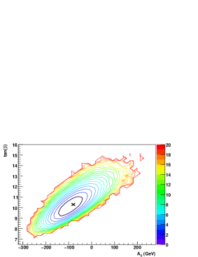
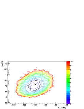
4.3.2 MSSM18

So far, we only considered SUSY models with specific assumptions on the SUSY breaking mechanism, namely mSUGRA and GMSB (for the fits to low energy measurements). As shown in Section 4.3.1 the LHC measurements together with LE measurements allow to derive tight constraints on the mSUGRA parameters if sufficient luminosity is accumulated at the LHC. In this section we investigate if it is possible to relax the strong constraints imposed on sparticle masses and couplings by the requirement of a specific breaking scenario. If it will be possible to measure the parameters of a more general model, like e. g. the MSSM18, at the electro-weak scale, properties of SUSY breaking models could be investigated in a bottom-up approach Blair:2002pg .

The results of a Markov Chain analysis of the MSSM18 model using LE and LHC observables with an integrated luminosity of 300 fb^-1 are shown in Table 25. Most parameters can be determined to the level of a few percent, except for third generation sfermion mass parameters, the trilinear coupling parameters $X_{\tau}=A_{\tau}-\mu\tan\beta$, $X_{b}=A_{b}-\mu\tan\beta$ and $X_{t}=A_{t}-\mu\cot\beta$ and the Higgs parameters $\tan\beta$ and $m_{A}$. The precision on the Higgs parameters $\tan\beta$ and $m_{A}$ suffers from the fact that for the analysed benchmark point SPS1a the heavy Higgs bosons are not directly accessible at the LHC.

Whereas for the mSUGRA fit to LE and LHC observables the impact of LE observables is almost negligible for 300 fb^-1 of LHC data, the situation for the MSSM18 is different. For some parameters the most stringent constraints still come from LE measurements. The most prominent examples are $\mathcal{B}(B\to s\gamma)$ and $(g-2)_{\mu}$. $\mathcal{B}(B\to s\gamma)$ is sensitive to the charged Higgs boson mass $m_{H^{\pm}}$ which in turn is tightly connected to the fitted SUSY parameter $m_{A}$. $(g-2)_{\mu}$ provides the most sensitive constraints on $M_{\tilde{\tau}_{L}}$ and $X_{\tau}$.

The obtained MSSM18 fit result can again be translated into a corresponding sparticle mass spectrum. This spectrum is presented in Figure 38. Again the masses in this Figure are model dependent predictions and do not represent direct mass measurements. Compared to the corresponding result for the more constrained mSUGRA model (Figure 35), some of the sparticle masses have significantly larger uncertainties in the MSSM18. This is particularly pronounced for the heavy Higgs boson masses, which are – as stated above – not directly accessible at the LHC for the considered SUSY benchmark point.

Although not studied explicitly for the MSSM18, one may expect that chain ambiguities may have a larger impact for this model than in the mSUGRA case. Since MSSM18 has more independently adjustable parameters, different decay chain interpretations can be more easily matched with the model due to the increased flexibility.

Figure 38: SUSY mass spectrum consistent with the existing low-energy measurements from Table 1 and the expected LHC measurements from Table 2 at ${\cal L}^{\mathrm{int}}=300\,\mathrm{fb}^{-1}$ for the MSSM18 model. The uncertainty ranges represent model dependent uncertainties of the sparticle masses and not direct mass measurements.

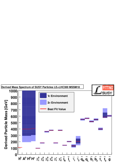
4.4 Low-Energy Observables, LHC and Expectations for ILC

The results of the previous sections show that the expected data of the LHC allow to obtain rather precise constraints on the mSUGRA parameters once sufficient luminosity is accumulated. However, for the MSSM18 scenario, the constraints severely diminish due to the increased theoretical freedom. The parameter uncertainties typically increase by a factor of 10 or more. Therefore an extrapolation of the SUSY parameters from the electro-weak scale to the GUT scale is afflicted with large uncertainties, if only low-energy, flavour physics, electro-weak precision, cosmological and LHC observables are used.

The expected measurements at the International Linear Collider, however, could dramatically increase the experimental precision of the measurements of sparticle masses and couplings. In addition to just increasing the experimental precision, the ILC is also expected to deliver a wealth of measurements of absolute branching fractions and cross-sections, many cross-section times branching fraction measurements, and many model-independent measurements of quantum numbers and CP-properties. This expected wealth of data, especially in a SUSY scenario with a rich phenomenology below a mass scale of 500 GeV, as predicted by the present measurements in Section 4.1, will strongly enhance the knowledge from the LHC due to the expected complementarity of ILC and LHC results Weiglein:2004hn .

In this section, first the expected precision on the parameters of the mSUGRA model is studied, followed by a detailed comparison of the results of the MSSM18 fit using only LE and LHC data with those obtained using LE, LHC and ILC data. Finally, the increase in precision is used to predict the cosmic cold dark matter relic density $\Omega_{\mathrm{CDM}}h^{2}$ from collider data, from fits excluding $\Omega_{\mathrm{CDM}}h^{2}$ itself from the list of observables.

4.4.1 mSUGRA

Table 24: Result of the fit of the mSUGRA model to the existing measurements and to the expected results from LHC with ${\cal L}^{\mathrm{int}}=300\,\mathrm{fb}^{-1}$ and ILC.

Parameter	Nominal value	Fit		Uncertainty
$\tan\beta$	10	9.999	$\pm$	0.050
$M_{1/2}$ (GeV)	250	249.999	$\pm$	0.076
$M_{0}$ (GeV)	100	100.003	$\pm$	0.064
$A_{0}$ (GeV)	$-$100	$-$100.0	$\pm$	2.4

Using the same available and expected measurements as in the fit using ${\cal L}^{\mathrm{int}}=300\,\mathrm{fb}^{-1}$ of LHC luminosity in Section 4.3.1, plus the expected ILC measurements discussed in Section 2.3, the fit of the mSUGRA model to the data of the SPS1a scenario is shown in Table 24. The comparison with the results without ILC in Table 22 shows the increase in precision by a factor of 5 to 10. However, the pure increase in precision for the fit of a high scale scenario is not the only improvement using ILC. First, possible deviations of the SUSY breaking implemented in Nature from a given GUT-scale SUSY breaking scenario, involving assumptions on unification, are much more visible using also ILC data. Second, the high accuracy and especially the larger variety (covering couplings, mixings, masses, widths and quantum numbers) and stronger model independence of the measurements allow to fit more general models of New Physics. This makes it possible to study the SUSY breaking mechanism using a bottom-up instead of a top-down approach.

4.4.2 MSSM18

As discussed in Section 4.3.2, the fit of the MSSM parameters at the SUSY breaking scale allows a bottom-up test of SUSY breaking and is independent of any assumptions about physics at the GUT scale. Section 4.3.2 showed that for the MSSM18 model, the parameter uncertainties from fits to existing data and expected LHC data are larger by at least one order of magnitude with respect to the fits of the mSUGRA scenario.

Table 25: Results of the Markov Chain MC analysis of the MSSM18 model using low energy observables, expected LHC results for ${\cal L}^{\mathrm{int}}=300\,\mathrm{fb}^{-1}$ and ILC.

Parameter	Nominal value	ILC Fit		$\sigma_{\mathrm{LE+LHC\,300}}$	$\sigma_{\mathrm{LE+LHC300+ILC}}$
$M_{\tilde{\ell}_{L}}$ (GeV)	194.31	194.315	$\pm$	6.4	0.068
$M_{\tilde{\ell}_{R}}$ (GeV)	135.76	135.758	$\pm$	10.5	0.071
$M_{\tilde{\tau}_{L}}$ (GeV)	193.52	193.46	$\pm$	43.0	0.33
$M_{\tilde{\tau}_{R}}$ (GeV)	133.43	133.45	$\pm$	38.2	0.35
$M_{\tilde{q}_{L}}$ (GeV)	527.57	527.61	$\pm$	3.4	0.64
$M_{\tilde{q}_{R}}$ (GeV)	509.14	509.3	$\pm$	9.0	9.0
$M_{\tilde{b}_{R}}$ (GeV)	504.01	504.2	$\pm$	33.3	2.4
$M_{\tilde{t}_{L}}$ (GeV)	481.69	481.6	$\pm$	15.5	1.5
$M_{\tilde{t}_{R}}$ (GeV)	409.12	409.2	$\pm$	103.8	1.6
$\tan\beta$	10	10.01	$\pm$	3.3	0.29
$\mu$ (GeV)	355.05	355.02	$\pm$	6.2	0.88
$X_{\tau}$ (GeV)	$-$3799.88	$-$3795.1	$\pm$	3053.5	46.6
$X_{t}$ (GeV)	$-$526.62	$-$526.8	$\pm$	299.2	4.7
$X_{b}$ (GeV)	$-$4314.33	$-$4252.1	$\pm$	5393.6	728.7
$M_{1}$ (GeV)	103.15	103.154	$\pm$	3.5	0.046
$M_{2}$ (GeV)	192.95	192.95	$\pm$	5.5	0.11
$M_{3}$ (GeV)	568.87	568.66	$\pm$	6.9	1.65
$m_{A}$ (GeV)	359.63	360.07	$\pm$	${}_{-99.3}^{+1181}$	1.83

Table 25 shows a comparison of the parameter uncertainties of the fits of the MSSM18 model using LE data in combination with ${\cal L}^{\mathrm{int}}=300\,\mathrm{fb}^{-1}$ of data at the LHC (LE+LHC300) and the latter plus the expected ILC results (LE+LHC300+ILC). The results of Markov Chain Monte Carlo scans and Toy Fits are in good agreement, therefore just the Markov Chain result is shown. For most parameters, the uncertainties decrease by approximately one order of magnitude. Interestingly, the increase in precision is not only limited to those parameters which are linked directly to observables at tree level. For example it is expected that the uncertainties of the gaugino mass parameters $M_{1}$ and $M_{2}$ are significantly decreased at ILC due to the increased precision on the $\tilde{\chi}^{0}_{1/2}$ and $\tilde{\chi}^{\pm}_{1}$ masses and the additional information from precise measurements of cross-sections times branching fractions for different polarisations. Also, the precision of the heavy Higgs sector parameter $m_{A}$ is expected to increase dramatically, since the heavy Higgs bosons $A$, $H$ and $H^{\pm}$ are not expected to be discovered at the LHC in this scenario, but to be precisely measured at the ILC Weiglein:2004hn . In contrast to those measurements, no additional experimental information is obtained on the gluino mass or the heavier squark masses at ILC. In any case, with the exception of $M_{\tilde{q}_{R}}$, all parameter uncertainties improve dramatically. The reason for this behaviour is the strong decrease of correlations. For example, the $\tilde{b}_{1/2}$ masses are determined by $M_{\tilde{q}_{L}}$ and $M_{\tilde{b}_{R}}$, but also by the off-diagonal elements $m_{b}X_{b}$ with $X_{b}=A_{b}-\mu\tan\beta$. Due to the strong increase in the determination of $\mu$ and $\tan\beta$ from the measurements in the Higgs sector (where also $A_{b}$ plays a role in loop effects) and the gaugino sector, also the precision of the parameter $M_{\tilde{b}_{R}}$ is strongly improved, although no direct measurement in the sbottom sector is made at the ILC in this scenario. This example highlights the importance of precision measurements for the detailed unravelling of the SUSY spectrum, and it is an example of the complementarity of LHC and ILC.

Figure 39: Derived mass distributions of the SUSY particles using existing measurements, expected results from LHC with ${\cal L}^{\mathrm{int}}=300\,\mathrm{fb}^{-1}$ and expected results from ILC.

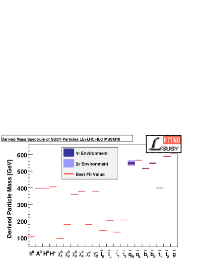
The resulting derived spectrum of sparticle masses is shown in Figure 39. It represents a very strong improvement over the results without ILC in Figure 38. The Higgs sector exhibits the strongest improvement due to the direct observation of heavy Higgs states. Apart from the squark mass $m_{\tilde{q}_{L}}$, solely governed by the parameter $M_{\tilde{q}_{R}}$, the uncertainties of all other derived masses increase dramatically.

Figure 40: Ratio of the predicted value of $\Omega_{\mathrm{pred}}h^{2}$ to the nominal value of $\Omega_{\mathrm{SPS1a}}h^{2}$ in the SPS1a scenario for a variety of Toy Fits without using $\Omega_{\mathrm{CDM}}h^{2}$ as an observable.

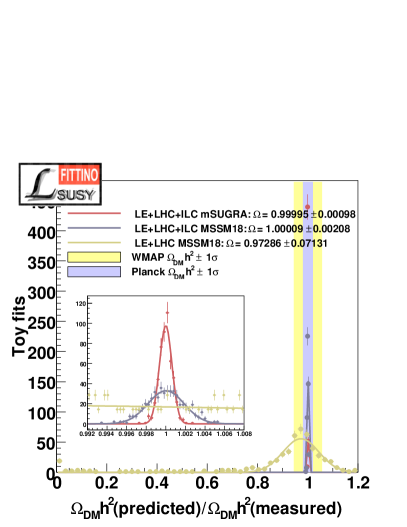
As a final test of the agreement between cosmology and collider data, and as a showcase for the predictive power of precision collider measurements, additional fits without $\Omega_{\mathrm{CDM}}h^{2}$ are performed with and without the use of ILC using the Toy Fit technique. The resulting predicted values of $\Omega_{\mathrm{CDM}}h^{2}$ are shown in Figure 40 and compared with the present and expected experimental precision of $\Omega_{\mathrm{CDM}}h^{2}$ from the WMAP Dunkley:2008ie and Planck Feng:2005uu data. The prediction of $\Omega_{\mathrm{CDM}}h^{2}$ from collider data without ILC in the MSSM18 model shows a long non-Gaussian tail down to $\Omega_{\mathrm{CDM}}h^{2}=0$. The Gaussian core of the distribution is one order of magnitude wider than the expected precision from the Planck satellite. Therefore witout ILC, the relic density constraints inferable from particle physics within the MSSM18 model do not match the precision of cosmological measurements.

In contrast to that, the result including ILC for the MSSM18 scenario achieves a relative precision on $(\Omega_{\mathrm{CDM}}^{\mathrm{pred}}h^{2})/(\Omega_{\mathrm{CDM}}^{\mathrm{meas}}h^{2})$ of $0.2\,\%$, which is an order of magnitude more precise than the expected Planck accuracy. An agreement between the collider result and the cosmological measurement would provide strong hints that SUSY LSPs make up the vast majority of dark matter and would allow to make predictions for direct dark matter search experiments. For comparison, the achievable accuracy on the relic density is also shown assuming mSUGRA. The uncertainty is improved again by a factor of two.

In summary, for a SUSY scenario in agreement with the present cosmological, low-energy and collider data, the ILC would tremendously improve the theoretical understanding of a SUSY model by improving the precision of bottom-up determinations of SUSY parameters without assumptions on unification and breaking mechanisms at the GUT scale. The precision would ensure that cosmological implications of New Physics could be predicted with a precision significantly better than the current and expected cosmological measurements.

5 Conclusions

We have performed a comprehensive study of current and future uncertainties and correlations of the parameters of supersymmetric models, i. e. the mSUGRA and GMSB model as well as the MSSM18.

For the case of LE data presently available we confirm the results of Buchmueller:2008qe leading to the conclusion that within the mSUGRA model, sparticles are predicted to be light enough for an early discovery at the LHC. In particular, the squark and gluino masses, which determine the major production cross-sections at the LHC are below 1 TeV at 68 % CL and below 1.6 TeV at 95 % CL. The most sensitive measurements are the muon anomalous magnetic moment $(g-2)_{\mu}$ and the cold dark matter density $\Omega_{\mathrm{CDM}}h^{2}$. For $(g-2)_{\mu}$ the results rely on the calculation of the hadronic vacuum corrections based on $e^{+}e^{-}$ cross-section data. Sparticle masses are less constrained for scenarios where the SM prediction of $(g-2)_{\mu}$ is closer to its measured value. This is currently the case for the prediction based on $\tau$-data for the hadronic vacuum corrections Davier:2009ag , where the heaviest sparticles are expected below 1.4 TeV at 68 % CL and 3 TeV at 95 % CL. With no deviation of $(g-2)_{\mu}$, sparticles are still constrained to lie below approximately 2 (3.5) TeV at 68 (95) % CL. A good fit of the data (excluding $\Omega_{\mathrm{CDM}}h^{2}$) can also be achieved within GMSB yielding sparticle masses approximately below 1.2 (2.0) TeV at 68 (95) % CL. This result shows that the feature of light sparticles is not exclusively true within mSUGRA, although it may not be true within the general MSSM. Furthermore the LE data and the value of $\Omega_{\mathrm{CDM}}h^{2}$ in particular point towards a small mass difference of the LSP and the NLSP which is $\tilde{\tau}_{1}$. The mass of the lightest Higgs boson is predicted to be just above the exclusion of the LEP experiments.

For the SPS1a parameter point, which provides a phenomenology rather similar to the region preferred by the LE fit we determined the prospects for parameter measurements at the LHC for a complete set of experimentally accessible and well-studied observables. Within mSUGRA, a coarse determination of the parameters can already be achieved with an integrated luminosity of 1 fb^-1. The precision can be significantly improved when LE data are combined with the early LHC measurements. For 300 fb^-1, a precision of better than 1 % can be achieved on $M_{0}$ and $M_{1/2}$. The parameter $\tan\beta$ ($A_{0}$) can be determined to 3.5 (11) % precision. At high luminosity the impact of LE data becomes small.

For the MSSM18, parameter determination is significantly more difficult and requires larger integrated luminosity. Nevertheless, for 300 fb^-1 a decent determination of all sparticle masses can be achieved to a few percent precision with the exception of $\tilde{t}_{2}$, $\tilde{\tau}_{2}$ and the heavy Higgs bosons. Here the inclusion of LE data still has significant impact, in particular in constraining third generation sparticles. With a linear collider like the ILC operating at up to 1 TeV, the MSSM18 can be reconstructed with a precision increased by approximately one order of magnitude.

It should be noted that the bulk region of the MSSM as exemplified in the SPS1a parameter point is certainly favourable for the prospects of parameter measurements at both the LHC and the ILC. For the LHC, various experimental studies of different parameter points exist, however no full analysis of more difficult regions exists to date. In particular in regions where long decay chains with charged leptons are suppressed, the reconstruction of SUSY parameters will be substantially more difficult and imprecise. However, given the constraints from LE data, such scenarios appear less likely. Given the smaller mass difference between sleptons and the lightest neutralino observed in the fit to the LE data when compared with SPS1a, a more detailed comprehensive experimental study of co-annihilation points at LHC would be beneficial.

In addition to these quantitative results we proposed some new methodological approaches to take care of ambiguities in the assignment of experimental observables to physical final states. It was shown, that in some cases these ambiguities may be translated into the uncertainty on the parameters when the ambiguities cannot be resolved statistically. We have also shown that the Bayesian and Frequentist interpretation of Markov Chain Monte Carlo lead to very similar results for fits including LHC data when flat priors are used in the Bayesian approach. For fits of LE data only, however, the two interpretations do not necessarily agree. It is observed that the Bayesian approach, which includes marginalisation of the hidden parameters requires a prohibitive amount of computing power. In such cases, only the Frequentist interpretation is exploited.

In the future, the technologies presented in this paper will be applied to a larger variety of models and finally to real data from the LHC. In addition, the proposed treatment of the assignment ambiguities will be extended to further possible self-consistent interpretations of the data and the resulting effect on parameter uncertainties and possible exclusions of assignments will be evaluated. It also is expected to be important to evaluate the effect of theoretical uncertainties stemming e. g. from missing higher order effects and differences between different implementations of RGE running in more detail. In addition to the uncertainties itself, the evaluation of correlations among theoretical uncertainties could be relevant. Finally, if SUSY is realised in Nature, sparticles could be discovered before the discovery of a SUSY Higgs boson. Therefore, the implementation of present and future limits on Higgs boson production in arbitrary models of New Physics, using Bechtle:2008jh could be important.

References

- (1) J. Wess and B. Zumino, Nucl. Phys. B 70 (1974) 39.
- (2) H. P. Nilles, Phys. Rept. 110 (1984) 1.
- (3) H. E. Haber and G. L. Kane, Phys. Rept. 117 (1985) 75.
- (4) L. Alvarez-Gaume, J. Polchinski and M. B. Wise, Nucl. Phys. B 221 (1983) 495.
- (5) L. E. Ibanez, Phys. Lett. B 118, 73 (1982).
- (6) J. R. Ellis, D. V. Nanopoulos and K. Tamvakis, Phys. Lett. B 121, 123 (1983).
- (7) K. Inoue, A. Kakuto, H. Komatsu and S. Takeshita, Prog. Theor. Phys. 68, 927 (1982) [Erratum-ibid. 70, 330 (1983)].
- (8) A. H. Chamseddine, R. L. Arnowitt and P. Nath, Phys. Rev. Lett. 49, 970 (1982).
- (9) L. Alvarez-Gaume, M. Claudson and M. B. Wise, Nucl. Phys. B 207 (1982) 96.
- (10) M. Dine and A. E. Nelson, Phys. Rev. D 48 (1993) 1277 [arXiv:hep-ph/9303230].
- (11) M. Dine, A. E. Nelson and Y. Shirman, Phys. Rev. D 51 (1995) 1362 [arXiv:hep-ph/9408384].
- (12) M. Dine, A. E. Nelson, Y. Nir and Y. Shirman, Phys. Rev. D 53 (1996) 2658 [arXiv:hep-ph/9507378].
- (13) G. Weiglein et al. [LHC/LC Study Group], Phys. Rept. 426 (2006) 47 [arXiv:hep-ph/0410364].
- (14) R. Lafaye, T. Plehn, M. Rauch and D. Zerwas, arXiv:0709.3985 [hep-ph].
- (15) P. Bechtle, K. Desch, W. Porod and P. Wienemann, Eur. Phys. J. C 46 (2006) 533 [arXiv:hep-ph/0511006].
- (16) C. G. Lester, M. A. Parker and M. J. White, JHEP 0601 (2006) 080 [arXiv:hep-ph/0508143].
- (17) P. Bechtle, K. Desch and P. Wienemann, Comput. Phys. Commun. 174 (2006) 47 [arXiv:hep-ph/0412012].
- (18) W. Porod, Comput. Phys. Commun. 153 (2003) 275 [arXiv:hep-ph/0301101].
- (19) P. Skands et al., JHEP 0407, 036 (2004) [arXiv:hep-ph/0311123].
- (20) B. Allanach et al., arXiv:0801.0045 [hep-ph].
- (21) T. Appelquist and J. Carazzone, Phys. Rev. D 11 (1975) 2856.
- (22) A. Dobado, M. J. Herrero and S. Penaranda, Eur. Phys. J. C 7 (1999) 313 [arXiv:hep-ph/9710313].
- (23) W. de Boer, A. Dabelstein, W. Hollik, W. Mosle and U. Schwickerath, Z. Phys. C 75 (1997) 627 [arXiv:hep-ph/9607286].
- (24) W. de Boer, A. Dabelstein, W. Hollik, W. Mosle and U. Schwickerath, arXiv:hep-ph/9609209.
- (25) G. C. Cho and K. Hagiwara, Nucl. Phys. B 574 (2000) 623 [arXiv:hep-ph/9912260].
- (26) G. C. Cho and K. Hagiwara, Phys. Lett. B 514 (2001) 123 [arXiv:hep-ph/0105037].
- (27) J. Erler and D. M. Pierce, Nucl. Phys. B 526 (1998) 53 [arXiv:hep-ph/9801238].
- (28) G. Altarelli, F. Caravaglios, G. F. Giudice, P. Gambino and G. Ridolfi, JHEP 0106 (2001) 018 [arXiv:hep-ph/0106029].
- (29) A. Djouadi, M. Drees and J. L. Kneur, JHEP 0108 (2001) 055 [arXiv:hep-ph/0107316].
- (30) W. de Boer, M. Huber, C. Sander and D. I. Kazakov, Phys. Lett. B 515, 283 (2001).
- (31) W. de Boer and C. Sander, Phys. Lett. B 585 (2004) 276 [arXiv:hep-ph/0307049].
- (32) G. Belanger, F. Boudjema, A. Cottrant, A. Pukhov and A. Semenov, Nucl. Phys. B 706 (2005) 411 [arXiv:hep-ph/0407218].
- (33) J. R. Ellis, K. A. Olive, Y. Santoso and V. C. Spanos, Phys. Rev. D 69 (2004) 095004 [arXiv:hep-ph/0310356].
- (34) J. R. Ellis, S. Heinemeyer, K. A. Olive and G. Weiglein, JHEP 0502 (2005) 013 [arXiv:hep-ph/0411216].
- (35) J. R. Ellis, D. V. Nanopoulos, K. A. Olive and Y. Santoso, Phys. Lett. B 633 (2006) 583 [arXiv:hep-ph/0509331].
- (36) J. R. Ellis, S. Heinemeyer, K. A. Olive and G. Weiglein, JHEP 0605 (2006) 005 [arXiv:hep-ph/0602220].
- (37) J. R. Ellis, S. Heinemeyer, K. A. Olive, A. M. Weber and G. Weiglein, JHEP 0708 (2007) 083 [arXiv:0706.0652 [hep-ph]].
- (38) E. A. Baltz and P. Gondolo, JHEP 0410 (2004) 052 [arXiv:hep-ph/0407039].
- (39) B. C. Allanach and C. G. Lester, Phys. Rev. D 73 (2006) 015013 [arXiv:hep-ph/0507283].
- (40) B. C. Allanach, Phys. Lett. B 635 (2006) 123 [arXiv:hep-ph/0601089].
- (41) B. C. Allanach, C. G. Lester and A. M. Weber, JHEP 0612 (2006) 065 [arXiv:hep-ph/0609295].
- (42) B. C. Allanach, K. Cranmer, C. G. Lester and A. M. Weber, JHEP 0708 (2007) 023 [arXiv:0705.0487 [hep-ph]].
- (43) R. R. de Austri, R. Trotta and L. Roszkowski, JHEP 0605 (2006) 002 [arXiv:hep-ph/0602028].
-
(44)
O. Buchmueller et al.,
JHEP 0809, 117 (2008)
[arXiv:0808.4128 [hep-ph]];
O. Buchmueller et al., Phys. Lett. B 657, 87 (2007) [arXiv:0707.3447 [hep-ph]]. - (45) H. Flacher, M. Goebel, J. Haller, A. Hocker, K. Moenig and J. Stelzer, Eur. Phys. J. C 60, 543 (2009) [arXiv:0811.0009 [hep-ph]].
- (46) [ALEPH Collaboration and DELPHI Collaboration and L3 Collaboration and OPAL Collaboration and SLD Collaboration], Phys. Rept. 427 (2006) 257 [arXiv:hep-ex/0509008].
- (47) E. Barberio et al. [Heavy Flavour Averaging Group (HFAG)], arXiv:hep-ex/0603003.
(48)
B. Aubert et al. [BABAR Collaboration],
Phys. Rev. Lett. 95, 041804 (2005)
[arXiv:hep-ex/0407038];
P. Chang, talk at ICHEP 2008, August 2008, Philadelphia, USA;
I. Adachi et al. [Belle Collaboration], arXiv:0809.3834 [hep-ex];
A. Gray et al. [HPQCD Collaboration], Phys. Rev. Lett. 95 (2005) 212001 [arXiv:hep-lat/0507015]. - (49) M. Bona et al. [UTfit Collaboration], JHEP 0803, 049 (2008) [arXiv:0707.0636 [hep-ph]].
- (50) M. Antonelli et al. [FlaviaNet Working Group on Kaon Decays], arXiv:0801.1817 [hep-ph].
- (51) A. V. Artamonov et al. [E949 Collaboration], Phys. Rev. Lett. 101, 191802 (2008) [arXiv:0808.2459 [hep-ex]].
- (52) G. W. Bennett et al. [Muon g-2 Collaboration], Phys. Rev. Lett. 92, 161802 (2004) [arXiv:hep-ex/0401008].
(53)
T. Moroi,
Phys. Rev. D 53 (1996) 6565
[Erratum-ibid. D 56 (1997) 4424]
[arXiv:hep-ph/9512396];
G. Degrassi and G. F. Giudice, Phys. Rev. D 58 (1998) 053007 [arXiv:hep-ph/9803384];
S. Heinemeyer, D. Stockinger and G. Weiglein, Nucl. Phys. B 690 (2004) 62 [arXiv:hep-ph/0312264];
S. Heinemeyer, D. Stockinger and G. Weiglein, Nucl. Phys. B 699 (2004) 103 [arXiv:hep-ph/0405255]. - (54) R. Barate et al. [LEP Working Group for Higgs boson searches and the LEP Collaborations], Phys. Lett. B 565 (2003) 61 [arXiv:hep-ex/0306033].
- (55) S. Schael et al. [LEP Working Group for Higgs boson searches and the LEP Collaborations], Eur. Phys. J. C 47 (2006) 547 [arXiv:hep-ex/0602042].
- (56) G. Degrassi, S. Heinemeyer, W. Hollik, P. Slavich and G. Weiglein, Eur. Phys. J. C 28, 133 (2003) [arXiv:hep-ph/0212020].
- (57) J. Dunkley et al. [WMAP Collaboration], Astrophys. J. Suppl. 180, 306 (2009) [arXiv:0803.0586 [astro-ph]].
- (58) C. Amsler et al. [Particle Data Group], Phys. Lett. B 667 (2008) 1.
- (59) [Tevatron Electroweak Working Group and CDF Collaboration and D0 Collaboration], arXiv:0808.1089 [hep-ex].
- (60) J. Charles et al. [CKMfitter Group], Eur. Phys. J. C 41 (2005) 1 [arXiv:hep-ph/0406184].
- (61) J. Z. Bai et al. [BES Collaboration], Phys. Rev. Lett. 88 (2002) 101802 [arXiv:hep-ex/0102003].
- (62) B. e. Lautrup, A. Peterman and E. de Rafael, Phys. Rept. 3, 193 (1972).
- (63) M. Davier, S. Eidelman, A. Hocker and Z. Zhang, Eur. Phys. J. C 31, 503 (2003) [arXiv:hep-ph/0308213].
- (64) S. Ghozzi and F. Jegerlehner, Phys. Lett. B 583 (2004) 222 [arXiv:hep-ph/0310181].
- (65) S. Heinemeyer, W. Hollik and G. Weiglein, Eur. Phys. J. C 9 (1999) 343 [arXiv:hep-ph/9812472].
(66)
J. R. Ellis, S. Heinemeyer, K. A. Olive and G. Weiglein,
Phys. Lett. B 515 (2001) 348
[arXiv:hep-ph/0105061];
S. Ambrosanio, A. Dedes, S. Heinemeyer, S. Su and G. Weiglein, Nucl. Phys. B 624, 3 (2002) [arXiv:hep-ph/0106255]. - (67) [CDF Collaboration and D0 Collaboration], arXiv:0903.4001 [hep-ex].
- (68) B. C. Allanach et al., in Proc. of the APS/DPF/DPB Summer Study on the Future of Particle Physics (Snowmass 2001) ed. N. Graf, In the Proceedings of APS / DPF / DPB Summer Study on the Future of Particle Physics (Snowmass 2001), Snowmass, Colorado, 30 Jun - 21 Jul 2001, pp P125, [arXiv:hep-ph/0202233].
- (69) B. K. Gjelsten, D. J. . Miller and P. Osland, JHEP 0412 (2004) 003 [arXiv:hep-ph/0410303].
- (70) C. G. Lester and D. J. Summers, Phys. Lett. B 463 (1999) 99 [arXiv:hep-ph/9906349].
- (71) A. Barr, C. Lester and P. Stephens, J. Phys. G 29 (2003) 2343 [arXiv:hep-ph/0304226].
- (72) M. M. Nojiri, G. Polesello and D. R. Tovey, arXiv:hep-ph/0312317.
- (73) B. C. Allanach, Comput. Phys. Commun. 143 (2002) 305 [arXiv:hep-ph/0104145].
(74)
M. Frank, T. Hahn, S. Heinemeyer, W. Hollik, H. Rzehak and G. Weiglein,
JHEP 0702, 047 (2007)
[arXiv:hep-ph/0611326];
S. Heinemeyer, W. Hollik and G. Weiglein, Comput. Phys. Commun. 124, 76 (2000) [arXiv:hep-ph/9812320]. -
(75)
G. Isidori, F. Mescia, P. Paradisi and D. Temes,
Phys. Rev. D 75, 115019 (2007)
[arXiv:hep-ph/0703035];
G. Isidori and P. Paradisi, Phys. Lett. B 639, 499 (2006) [arXiv:hep-ph/0605012]. -
(76)
F. Mahmoudi,
arXiv:0808.3144 [hep-ph];
F. Mahmoudi, Comput. Phys. Commun. 178, 745 (2008) [arXiv:0710.2067 [hep-ph]]. - (77) S. Heinemeyer, W. Hollik, D. Stockinger, A. M. Weber and G. Weiglein, JHEP 0608 (2006) 052 [arXiv:hep-ph/0604147].
- (78) S. Heinemeyer, W. Hollik, A. M. Weber and G. Weiglein, JHEP 0804, 039 (2008) [arXiv:0710.2972 [hep-ph]].
(79)
G. Belanger, F. Boudjema, A. Pukhov and A. Semenov,
Comput. Phys. Commun. 176, 367 (2007)
[arXiv:hep-ph/0607059];
G. Belanger, F. Boudjema, A. Pukhov and A. Semenov, Comput. Phys. Commun. 174, 577 (2006) [arXiv:hep-ph/0405253];
G. Belanger, F. Boudjema, A. Pukhov and A. Semenov, Comput. Phys. Commun. 149, 103 (2002) [arXiv:hep-ph/0112278]. - (80) B. C. Allanach, S. Kraml and W. Porod, JHEP 0303 (2003) 016 [arXiv:hep-ph/0302102].
- (81) J. A. Aguilar-Saavedra et al., Eur. Phys. J. C 46 (2006) 43 [arXiv:hep-ph/0511344].
- (82) F. James and M. Roos, Comput. Phys. Commun. 10, 343 (1975).
- (83) N. Metropolis, A. W. Rosenbluth, M. N. Rosenbluth, A. H. Teller and E. Teller, J. Chem. Phys. 21 (1953) 1087.
- (84) D. MacKay, Information Theory, Inference, and Learning Algorithms, Cambridge University Press (2003).
- (85) S. S. AbdusSalam, B. C. Allanach, F. Quevedo, F. Feroz and M. Hobson, arXiv:0904.2548 [hep-ph].
- (86) see e. g. R. J. Barlow, “Statistics”, John Wiley and Sons, Chichester, 1989
- (87) G. Aad et al. [The ATLAS Collaboration], arXiv:0901.0512 [Unknown].
- (88) G. L. Bayatian et al. [CMS Collaboration], J. Phys. G 34, 995 (2007).
- (89) [LEP Collaborations and Tevatron Collaborations and SLD Collaboration], arXiv:0811.4682 [hep-ex].
(90)
A. Heister et al. [ALEPH Collaboration],
Phys. Lett. B 583 (2004) 247;
[LEP Collaborations], LEPSUSYWG/04-07.1, (http://lepsusy.web.cern.ch/lepsusy/www/ lsp_cmssm_summer04/cMSSM_final.html), obtained 06/22/2009. - (91) D. Stockinger, Nucl. Phys. Proc. Suppl. 181-182 (2008) 32.
- (92) M. Passera, Pramana 72 (2009) 195.
- (93) F. Jegerlehner and A. Nyffeler, Phys. Rept. 477 (2009) 1 [arXiv:0902.3360 [hep-ph]].
- (94) M. Davier et al., arXiv:0906.5443 [hep-ph].
- (95) J. A. Aguilar-Saavedra et al. [ECFA/DESY LC Physics Working Group], arXiv:hep-ph/0106315.
- (96) V. M. Abazov et al. [D0 Collaboration], arXiv:0901.0646 [hep-ex].
- (97) T. Aaltonen et al. [CDF Collaboration], arXiv:0903.2618 [hep-ex].
(98)
Phys. Lett. B 526 (2002) 206
[arXiv:hep-ex/0112011];
J. Abdallah et al. [DELPHI Collaboration], Eur. Phys. J. C 31 (2004) 421 [arXiv:hep-ex/0311019];
P. Achard et al. [L3 Collaboration], Phys. Lett. B 580 (2004) 37 [arXiv:hep-ex/0310007];
G. Abbiendi et al. [OPAL Collaboration], Eur. Phys. J. C 32, 453 (2004) [arXiv:hep-ex/0309014]. -
(99)
E. Pierpaoli, S. Borgani, A. Masiero and M. Yamaguchi,
Phys. Rev. D 57 (1998) 2089
[arXiv:astro-ph/9709047];
M. Viel, J. Lesgourgues, M. G. Haehnelt, S. Matarrese and A. Riotto, Phys. Rev. D 71 (2005) 063534 [arXiv:astro-ph/0501562]. - (100) F. Staub, W. Porod and J. Niemeyer, arXiv:0907.0530 [hep-ph].
(101)
R. L. Culbertson et al. [SUSY Working Group Collaboration],
arXiv:hep-ph/0008070;
P. Fayet, Phys. Lett. B 84, 416 (1979);
P. Fayet, Phys. Lett. B 70, 461 (1977). - (102) G. A. Blair, W. Porod and P. M. Zerwas, Eur. Phys. J. C 27 (2003) 263 [arXiv:hep-ph/0210058].
- (103) J. L. Feng, J. Phys. G 32 (2006) R1 [arXiv:astro-ph/0511043].
- (104) P. Bechtle, O. Brein, S. Heinemeyer, G. Weiglein and K. E. Williams, arXiv:0811.4169 [hep-ph].