DNA-Protein Binding Rates: Bending Fluctuation and Hydrodynamic Coupling Effects
Abstract
We investigate diffusion-limited reactions between a diffusing particle and a target site on a semiflexible polymer, a key factor determining the kinetics of DNA-protein binding and polymerization of cytoskeletal filaments. Our theory focuses on two competing effects: polymer shape fluctuations, which speed up association, and the hydrodynamic coupling between the diffusing particle and the chain, which slows down association. Polymer bending fluctuations are described using a mean field dynamical theory, while the hydrodynamic coupling between polymer and particle is incorporated through a simple heuristic approximation. Both of these we validate through comparison with Brownian dynamics simulations. Neither of the effects has been fully considered before in the biophysical context, and we show they are necessary to form accurate estimates of reaction processes. The association rate depends on the stiffness of the polymer and the particle size, exhibiting a maximum for intermediate persistence length and a minimum for intermediate particle radius. In the parameter range relevant to DNA-protein binding, the rate increase is up to compared to the Smoluchowski result for simple center-of-mass motion. The quantitative predictions made by the theory can be tested experimentally.
I Introduction
Reactions between semiflexible polymers and small molecules are ubiquitous in cells, playing a crucial role in a large number of biological processes: examples include the interaction of gene-regulating proteins with specific target sites on DNA, and the polymerization of DNA or structural proteins such as actin and tubulin. Many of these reactions are diffusion-limited [1]—the activation free-energy is negligible compared to the thermal energy and the reaction is not hindered by other steric or conformational factors—so the overall association speed therefore depends on the rate at which the reactive molecules approach each other.
DNA-protein interaction has been the most widely studied process of this type [2, 3], attracting attention since the first measurement of the reaction rate between the lac repressor and operator [4] revealed that it far exceeds the 3D diffusion-limit. The quest to identify the underlying mechanism culminated in the seminal idea of facilitated diffusion by Berg, Winter, and von Hippel [5, 6, 7], but the general description of DNA-protein interaction is still far from complete. Although recent single molecule experiments show evidence that certain proteins indeed make use of facilitated diffusion [8, 9], the majority of measured reaction rates for DNA-binding proteins [2, 10, 11] do not exceed the Smoluchowski result for 3D diffusion [12]. Thus recent years have seen extensive theoretical efforts [13, 14, 15, 16, 17] revisiting the underlying assumptions of facilitated diffusion, and examining it anew in response to experimental advances.
Diffusion-controlled reactions with targets on flexible polymers are a well-established subject in polymer physics, with general analytical frameworks developed by Wilemski and Fixman [18, 19], and Szabo, Schulten, and Schulten [20] decades ago. Using the Wilemski-Fixman approach and a Gaussian model for circular polymers, a study by Berg looked at the influence of internal DNA motion on the binding of proteins [21]. But little is known about the role of chain stiffness, and both Berg’s study and the classic polymer reaction rate theories do not include hydrodynamics. This is a significant oversight, because solvent-mediated interactions modify not only the approach of the particle to the target site, but also the fluctuation of the entire polymer contour, and thus all time scales involved in the dynamics. Moreover, the two effects are in opposition: polymer fluctuations lead to the target site exploring a larger configurational space than simple center-of-mass diffusion, and hence the association rate is enhanced; the hydrodynamic coupling between the particle and coil, on the other hand, reduces their relative mobility, decreasing the rate. The observed binding rate is a subtle competition between these two phenomena. As experiments are providing an ever more detailed picture of biological reactions at the single molecule level, we need theories that begin to grapple with the full complexity of polymer-particle diffusive motion.
The paper is organized as follows: in Sec. II we briefly review the renewal approach used to derive first-passage times and association rates in the diffusion-controlled limit; a discussion of a few effects going beyond this limit is contained in Appendix A. The theoretical analysis of the dynamics in the polymer-particle system makes use of a mean field approach for the polymer dynamics and a heuristic approximation for inter-particle hydrodynamics. The main results are shown in Sec. II, while a brief review of the theory and calculational details are postponed to the appendices B and C. The Brownian dynamics (BD) simulation method used to independently test the theoretical description is described in Sec. III. The detailed validation of the theory through BD simulation results is presented in Sec. IV. We then investigate how the mechanical characteristics of the semiflexible polymer—the contour and persistence lengths—affect the reaction rate. Ultimately our theory yields quantitative predictions that can be tested empirically. Sec. V summarizes the main results and offers suggestions for future experiments.
II Theory
Diffusion-controlled reaction rates
In general, association rates are calculated by finding the steady-state solution of a diffusion equation with absorbing boundary conditions [22, 23]. In our case, we can employ the simpler renewal approach [24, 25], which avoids the necessity of imposing absorbing boundaries: first passage times and binding rates can be directly extracted from the solution of the unbounded problem, i.e. the dynamic Green’s function describing the time evolution of the relative distance between reactants subject to diffusive motion. The renewal approach is in principle equivalent to the Wilemski-Fixman formalism, and they share the same underlying approximations [26, 27]: (i) the Green’s function for the time evolution of the particle-target distance is assumed to be that of a stationary Markov process; (ii) excluded-volume between the reactants is ignored. In the following we briefly review the main aspects of the approach.
For a stochastic process in one dimension, the Green’s function specifies the probability to find the particle at at time given a starting point at time . If we are interested in paths that reach a boundary point in time , the corresponding transition probability can be written as a convolution,
| (1) |
where is the first passage time distribution: the probability of reaching in time starting from at without passing through along the way. A Laplace transformation acting on the time variable leads to
| (2) |
where Laplace transforms are denoted by . Note that is the Green’s function in the absence of absorbing boundary conditions; we assume only that the probability vanishes at .
To investigate the role of polymer fluctuations and of hydrodynamics on the reaction rates of diffusion controlled reactions, we consider an idealized situation: the only parameter relevant for the binding process then is the radial distance between the reactants meaning that the problem is effectively reduced to one dimension. Deviations from this simple picture and their impact on the association rates are discussed in Appendix A. In the case of perfect absorption, particles bind when they collide for the first time—when the relative distance reaches the absorption radius . As a result, the binding rate can be obtained from the first passage time distribution by integrating over all possible initial separations:
| (3) |
The steady-state rate reached at long times is extracted from the Laplace transform using the final value theorem:
| (4) |
For the simple case of two kinds of uncoupled Brownian particles with diffusion constants and , the radial Green’s function, which will explicitely be shown in the next section (Eqs. 10-11), can be easily written down and the result for the first passage time distribution in Laplace space reads
| (5) |
with total diffusion constant . Applying Eq. 3, which corresponds to imposing uniform initial concentrations at time , one obtains the association rate:
| (6) |
which at long times reduces to the well-known Smoluchowski rate [12] constituting the upper limit for reaction rates governed by Brownian diffusion in three dimensions.
For the more complicated polymer-particle case, the renewal method works analogously, but the Laplace transforms must be carried out numerically using standard numerical techniques [28]: the Laplace-transformation of the numerator in Eq. 2 is performed with the routine gsl_integration_qags with upper integration boundary , while the Laplace transform of the denominator in Eq. 2 and the numerical integration over initial separations in Eq. 3 are obtained using the routine gsl_integration_qagiu; a workspace of intervals was allocated for all these routines and the relative and absolute error bounds were set to . For the numerical implementation of the final value theorem in Eq. 4 a value ( being the diffusional time scale of a spherical particle of radius in a solvent of viscosity ) proved appropriate: within this range the numerical evaluation of the steady state Smoluchowski-rate coincided with the analytic result within a typical relative accuracy of . Results of the renewal approach applied to DNA-protein dynamics are presented in Sec. IV.
Dynamic Green’s functions
As outlined above the knowledge of dynamic Green’s functions specifying the probability that a radial distance between two objects is realized at time after starting at a radial distance allows the calculation of association rates.
The first step towards the description of the polymer-particle system consists in the analysis of the polymer motion itself: The dynamics of semiflexible polymers including hydrodynamics can be captured by a mean field theory discussed in detail in Ref. [29], where the model was shown to provide an accurate description of internal polymer kinetics, validated through extensive comparisons with BD simulations. Moreover, the theory can be independently tested by comparison to recent fluorescence correlation spectroscopy experiments [30]: without any fitting parameters, it exhibits excellent agreement for the mean square displacement (MSD) of tagged ends of single dsDNA fragments diffusing in solution [31].
Here we demonstrate that the mean field approach in addition also exhibits excellent agreement for the dynamic Green’s function characterizing the motion of specific points on the polymer contour when comparing theory and BD results. A short overview of the theory and details concerning the derivation can be found in Appendix B; the result of the calculation involving a normal mode expansion is a Gaussian Green’s function specifying the conditional probability that a point on the polymer contour (specified by the arc-length variable ) reaches spatial position in time given a start at :
| (7) | ||||
| (8) |
In Eq. 8 denotes the center-of-mass diffusion constant of the polymer coil and is given in Appendix B. The values of the fluctuation dissipation parameters and of the inverse relaxation times result from the (numerical) evaluation of the hydrodynamic interaction tensor; the normal modes with mode number additionally depend on polymer parameters, i.e. contour length and persistence length . The variance in Eq. 8 thus has contributions of the center-of-mass motion of the entire polymer coil and of internal fluctuations of the contour: on large time scales the variance reduces to and hence the motion is dominated by the Brownian diffusion of the polymer’s center-of-mass, for smaller times, however, the contribution from internal polymer modes becomes important. The radial Green’s function for a particle starting at is obtained by integrating over the surface of a sphere of radius :
| (9) |
In Sec. IV we compare the time evolution of this transition probability for the case of the end-monomer () to BD simulation results.
Hydrodynamic interactions influence the relative motion of diffusing objects: these interactions are included in our analytic approach by a heuristic approximation, which is motivated for the case of two spherical particles and for the case of a single diffusing particle and a specific target site on a polymer in Appendix C.
In general, the dynamic Green’s function takes the form of a Gaussian centered at the initial separation ; the integration over a sphere of radius leads to the radial Green’s function:
| (10) |
where the superscript discriminates between radial Green’s functions without and with hydrodynamics. In total, we distinguish four cases in our analysis: two spherical particles without hydrodynamics (i) and with hydrodynamics (ii), and a spherical particle and a specific target point on a semiflexible polymer without hydrodynamics (iii) and with hydrodynamics (iv), for which the respective variances are:
| (i) | (11) | |||
| (ii) | (12) | |||
| (iii) | (13) | |||
| (iv) | (14) |
where and are the diffusion constants in the case of relative diffusion of two spherical particles, is the diffusion constant of the free particle in the case of the polymer-particle reaction, is the polymer’s center-of-mass diffusion constant and the sums over the mode numbers again characterize the polymer’s contour fluctuations (compare Eq. 8). The slowing down of the relative motion due to hydrodynamics is reflected by the effective coupling parameter , which is motivated and shown in its full functional form in Appendix C. The non-hydrodynamic and hydrodynamic Green’s functions for the two systems we consider are compared to BD results in Sec. IV.
III Brownian dynamics simulations
To test the analytic results of Sec. II, we simulate a semiflexible polymer in solution adopting a standard Brownian dynamics scheme [32], in which the polymer is modeled as a chain of beads of radius . For the low Reynolds number regime, the Langevin equation governing the time evolution of the position of bead is given by
| (15) |
The long-range hydrodynamic interactions—the fact that a force acting on bead creates a flow-field affecting the motion of bead —are described by the Rotne-Prager mobility matrix [33]:
| (16) | ||||
| (17) |
where , , is the identity matrix, and is the Stokes self-mobility of a sphere of radius in a solvent of viscosity . The stochastic contributions in Eq. 15 are assumed to be Gaussian random vectors which are hydrodynamically correlated according to the fluctuation-dissipation theorem:
| (18) |
The inter-bead potential determining the configuration-dependent forces, where
| (19) |
consists of a shifted harmonic potential between adjacent beads of strength , a bending potential of strength between adjacent bonds, and a pairwise truncated Lennard-Jones potential of strength . Here is the angle between the bond vectors and . The first term in the worm-like chain potential keeps the contour length approximately fixed, while the second one with modulus takes care of the bending stiffness of the chain. The repulsive Lennard-Jones potential prevents significant bead overlap, which is a source of numerical instabilities. In Sec. IV, where we model the motion of a free particle (i.e. a protein or free monomer) relative to the polymer chain, the particle is represented by an additional bead, not connected to the polymer chain, and subject only to hydrodynamic interactions between the particle and the chain. We do not account for steric interactions between particle and polymer in order to simplify the comparison with the theoretical results where such effects cannot be properly included. A short discussion of excluded-volume effects is given in Appendix A. To avoid numerical instabilities in situations where the free particle overlaps with the polymer, in this case we use the Rotne-Prager-Yamakawa tensor [34], which modifies Eq. 17 for overlapping beads:
| (20) |
Eq. 15 is discretized and integrated numerically using the Euler algorithm. The correlated stochastic contributions of Eq. 18 are obtained from uncorrelated Gaussian noise by means of a Cholesky decomposition of the hydrodynamic matrix . In all the results below, lengths are measured in units of , energies in units of and time in units of . The time step is , and a typical simulation lasts steps, after an initial thermalization period of steps. To reduce computational costs the Cholesky decomposition is only performed every 5 time steps. For a given chain length and persistence length , the quantities of interest are averaged over different trajectories until the convergence is satisfactory.
IV Results
In order to validate the various analytical approaches described in Sec. II, we test them against BD simulations. Since the binding rates depend sensitively on having good estimates for the Green’s functions, we will focus on showing that the MFT approximation for the transition probabilities can reproduce the crucial physical effects: (i) the influence of internal polymer modes on the diffusion of the target site; (ii) the slow-down of relative motion between the free particle and target due to hydrodynamics. For simplicity, we concentrate in our analysis on one particular target site, the end-monomer of the chain. This has special relevance in biological processes, for example in the case of polymerization. Nevertheless, our theoretical approach is equally applicable to other target positions along the polymer contour: the results are similar though changes in the association rates are clearly less drastic because of the reduced mobility of target sites in the middle of the chain compared to the one at the chain’s end.
Polymer motion
We begin by considering just the internal relaxation of a polymer of total contour length : the radial Green’s function of Eqs. 8-9 describing the diffusive motion of the polymer end-point (). In Fig. 1 we compare this analytical MFT expression for to histograms extracted from simulations of a chain with , .
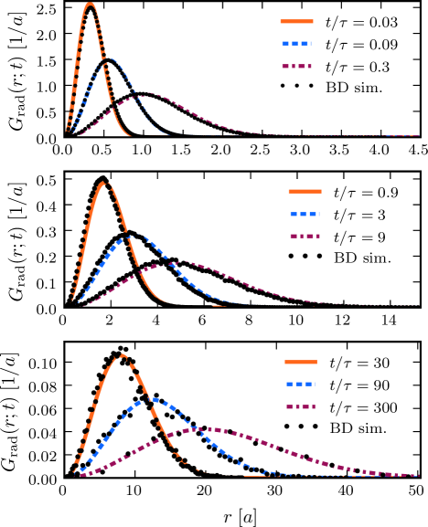
The histograms are based on the analysis of 25 independent trajectories, each with steps. The time evolution of the probability distribution is in excellent agreement with (Eqs. 8 and 9) over time scales spanning four orders of magnitude. Note that the largest time-scale considered () is less than the largest relaxation time of the polymer, , meaning that internal fluctuations dominate the polymer motion throughout this entire time range; the time evolution is illustrated more directly in the movie linked in Fig. 2 showing the remarkable agreement, even in the tails of the distribution (which are visible on the logarithmic scale spanning seven decades of magnitude).
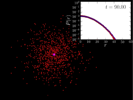
Our comparison here is more detailed than in the earlier MFT study of Ref. [29], since we consider the full transition probability and not just the end-point MSD. But the conclusion is the same: the MFT provides a highly accurate picture of internal polymer dynamics.
Relative motion of two spherical particles including hydrodynamics
Since the heuristic estimate for the hydrodynamic Green’s function of two freely diffusing particles (Eqs. 10 and 12) is the basis of our approach to polymer-particle interactions, we need to check that this estimate is reasonable. For this purpose, we performed hydrodynamic BD simulations of two single spheres of radius and extracted histograms from the variation of the inter-bead distance over time. In total 2400 independent trajectories were calculated, each starting at a distance and lasting time steps. For given separations and , relevant transition events were identified, i.e. parts of the trajectories starting at a certain distance and ending at , where is the histogram binwidth. These were used to estimate the probability distribution corresponding to . In Fig. 3 we show the BD simulation results for and various together with (Eqs. 10 and 12) and the hydrodynamically decoupled Green’s function (Eqs. 10 and 11). Analogous results for an initial separation are shown in Fig. 4.
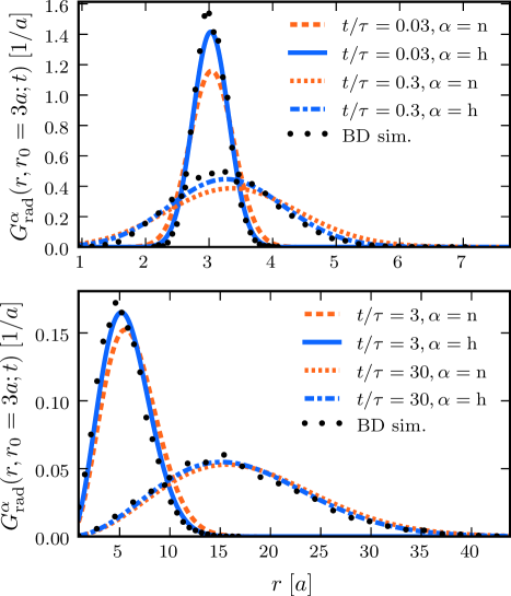
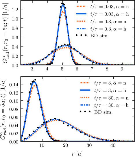
The inhibition of relative motion due to hydrodynamics is clearly evident at short times: the distributions from the simulations are more narrowly peaked than the decoupled results, which spread out noticeably faster. The slowing down is correctly reproduced in the curves, though it is slightly underestimated when compared to the simulation data. Despite the simplicity of the underlying approximation, still captures the essential features of the interaction. For longer times, when the inter-particle distance has become large and hydrodynamics plays a smaller role, converges to , and both agree with the BD results.
Relative motion of a polymer and a spherical particle including hydrodynamics
The final test for our Green’s function approach concerns the approximate description of polymer-particle relative motion, contained in Eqs. 10 and 14. To extract the corresponding transition probabilities from BD simulations, we take a polymer with , , allow it to thermalize, and then add a single free particle of radius that has no excluded-volume, but is hydrodynamically coupled to the polymer beads. The particle is positioned at an initial distance from one of the polymer ends, and data is collected over time steps. This procedure is repeated to obtain 2500 independent trajectories. As before, relevant transition events are used to determine the probability distribution for diffusing from a separation to in time . The results, plotted in Fig. 5 for and in Fig. 6 for , are qualitatively similar to the case of two particles: compared to the non-hydrodynamic case we see a reduced relative mobility between the target site and the particle for small separations.
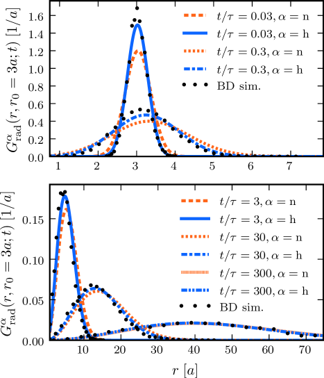
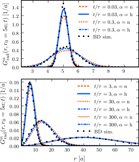
The hydrodynamic Green’s function is quite close to the simulation results, again slightly underestimating the strength of the coupling. However, given the complexity of the correlations between the particle and the entire polymer coil, it is notable that we are able to get good quantitative agreement. Since the association rates are derived directly from this Green’s function, we conclude that we should be able to obtain realistic estimates for the reaction process.
Association rates
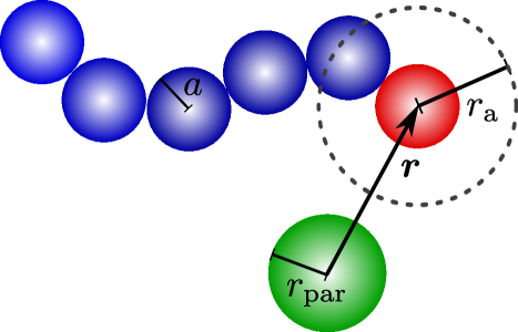
The diffusion-limited reaction we consider is schematically illustrated in Fig. 7: free particles are absorbed by the reactive end-monomer of a chain as soon as the separation reaches the absorption radius .
The association rate is calculated from the renewal approach in Sec. II, with the only input being the radial Green’s functions for the relative motion of the particle and the chain end (Eqs. 10 and 14).
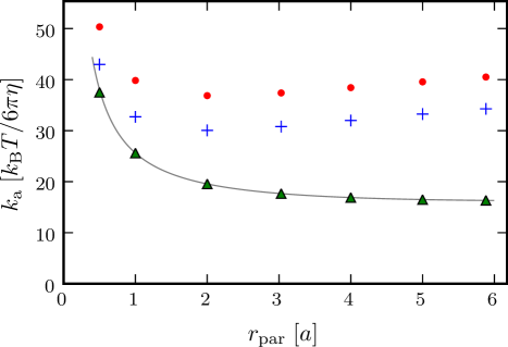
Since polymer fluctuations and the polymer-particle hydrodynamic coupling have competing effects on the association rate, it will be instructive to start with the simple case where the hydrodynamic coupling has been turned off, i.e. we use the non-hydrodynamic Green’s function of Eqs. 10 and 13. The resulting association rate as a function of particle radius for a polymer with , is marked by red dots in Fig. 8.
(For DNA, where nm and nm, this would correspond to a strand of length 1 m.) The Smoluchowski rate,
| (21) |
which involves only the center-of-mass motion of the polymer coil and particle, is shown as a line with the polymer diffusion constant taken from the MFT expansion in Appendix B. The corresponding numerical results of the renewal approach shown as green triangles are based on Eqs. 10 and 11 and again using from Appendix B. The Smoluchowski value is the standard point of reference when considering DNA-protein interaction [35]. Clearly, internal polymer fluctuations have a significant impact, enhancing the association rates by relative to over the range ; the minimum at for the rates with internal polymer motion indicates that the effect of larger absorption radius with increasing quickly dominates the one of decreasing diffusion constant .
In the absence of hydrodynamics, we can use an earlier result of Berg [21] to do a consistency check on the renewal approach derivation of the association rates. For the case of a Gaussian Green’s function, and assuming a Gaussian sink profile instead of a perfectly absorbing boundary at , Berg derived an expression for the association rate in terms of the relative non-hydrodynamic variance :
| (22) |
Plugging from Eq. 13 into Eq. 22, we recover the non-hydrodynamic rates shown in Fig. 8 within a difference of 5% (comparison not shown).
When hydrodynamic interactions are included together with internal polymer motion ( of Eqs. 10 and 14 is used instead of of Eqs. 10 and 13), the association rates are smaller than in the non-hydrodynamic case, as seen in the data marked by blue crosses in Fig. 8. This is due to the inhibited mobility between the particle and the target at short distances. However the rate decrease is only , so the overall association rate is still larger than the Smoluchowski result for the range of particle sizes considered. The magnitude of the rate decrease is comparable to previous estimates derived for the simpler problem of a reaction between two spherical particles: Friedman obtained a reduction due to hydrodynamics [36], Deutch and Felderhof saw a drop-off [37], and Wolynes and Deutch predicted a decrease by [38].
Since the conformational fluctuations depend on the mechanical properties of the chain, it is natural that the association rates will vary with the parameters and that characterize the semiflexible polymer. In Fig. 9 we show contour diagrams of the association rate in terms of and for two different particle radii: in the top panel, as would be the case in a polymerization process, and in the bottom panel, which corresponds to an average protein size for the case of DNA-protein interaction (with ). Fig. 10 depicts the same data, but in terms of percent rate increase over the Smoluchowski result of Eq. 21.
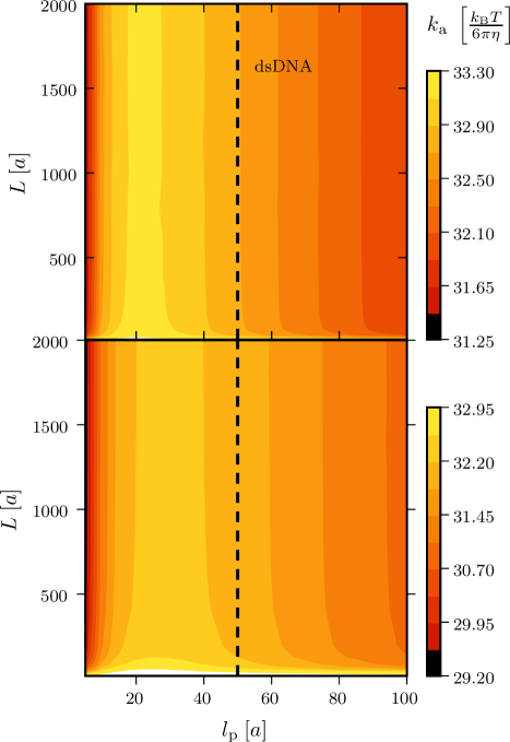
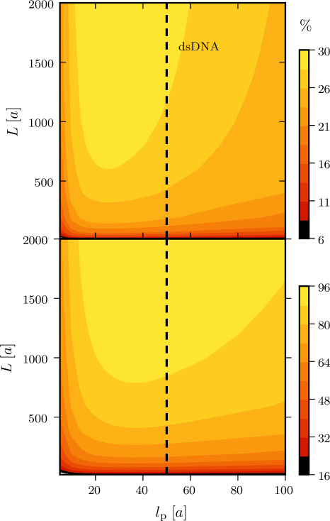
Interestingly, while the absolute rate in Fig. 9 is almost independent of for , it does show a slight maximum for when and when . This behavior as a function of is an intrinsic property of the polymer, because it appears also in the absence of hydrodynamic coupling (data not shown). This means that there is an optimal persistence length at which the chain reactivity is maximised, and interestingly this optimum is not far from the actual DNA persistence length of . The maximum is more prominent in the relative rates of Fig. 10, where the increase compared to rises sharply to () and () for long polymers with including double-stranded DNA ().
V Discussion and summary
In this paper, we have studied the association of free particles and a target site on a semiflexible polymer—a class of diffusion-limited reactions of wide biological relevance, whether in polymerization of biomolecules or gene regulation by DNA-binding proteins. We focused on two competing effects that are, with the lone exception of the segmental diffusion considered in Ref. [21], entirely neglected in existing theories for these processes: the bending fluctuations of the polymer in equilibrium, which enhance the association rate, and the hydrodynamics between the polymer and particle, which reduces it. Quantifying the fluctuations required an accurate description of internal polymer motion, available through the mean field theory of semiflexible polymer dynamics. For the hydrodynamics, we developed a simple heuristic estimate to model the decrease in mobility when two diffusing objects approach each other. The end result of the competition sensitively depends on the mechanical properties of the polymer and the size of the reactive particle: we see a maximal increase over the Smoluchowski rate for persistence lengths ; this increase is for the case of small particles, and for particle sizes typical of regulatory proteins. As a function of particle size, the reaction rate displays a minimum at a particle radius equal to the polymer diameter; for larger proteins the probability of hitting the DNA increases.
Although based on experimental evidence it is generally assumed that the binding of proteins to DNA is a diffusion-limited process [2] (and Refs. therein), recent studies in the slightly different context of protein assisted interior loop formation of DNA [39, 40] indicate that this assumption is probably not justified for all kinds of DNA-protein systems. Within our approach we have neglected the possibility of encounters between the protein and the target site on the DNA that do not immediately lead to a reaction, for example due to orientational constraints. This is clearly an oversimplification, which however can be approximately rectified by a reaction factor (see Appendix A).
Directly testing our theoretical predictions may be possible with existing experimental techniques. In particular, one can study the role of polymer fluctuations on association rates by comparing two different setups involving bimolecular diffusion-limited reactions, shown schematically in Fig. 11.
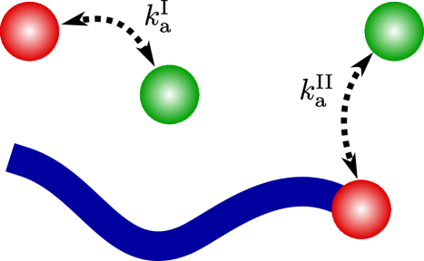
In scenario I both reactants are free in solution, while in scenario II one of the reactants is bound to the end of a semiflexible polymer. The corresponding rates and could be measured through simple kinetic experiments or using fluorescence microscopy. In the latter case, the reactants would be fluorophores and quencher molecules, and the rate of the diffusion-limited quenching reaction can be extracted from the decay of the total fluorescence signal over time. As shown in Table I, our theory predicts a ratio for the two scenarios using and a 1 m strand of DNA.
| Rate estimates including | |||
|---|---|---|---|
| center of mass motion | 50.27 | 25.14 | 0.5 |
| plus internal polymer motion | - | 39.83 | - |
| plus hydrodynamics | 42.52 | 32.71 | 0.77 |
This is clearly distinguishable from the Smoluchowski prediction, , which ignores hydrodynamics and internal fluctuations.
VI Acknowledgements
The authors would like to thank Ana-Maria Florescu and Marc Joyeux for useful discussions, and the DFG (grants NE 810/7 and SFB 863) for financial support.
Appendix Appendix A Additional Effects on the Association Rates
Throughout this paper we have considered an idealized picture of the association process assuming that a reaction takes place as soon as the radial distance reaches the absorption radius . A more realistic description should take into account a number of other factors: (i) molecules are in general not equally reactive on their entire surface, i.e. binding also depends on the relative orientation of the reactants; (ii) the correct relative orientation alone might not directly lead to binding due to additional requirements, e.g. conformational changes of the molecules. In addition we have assumed that the polymer-particle dynamics is purely diffusive; deviations from this behavior might be caused by (iii) excluded-volume effects between the particle and non-target monomers of the polymer together with (iv) electrostatic interactions between the particle and polymer. Due to all these effects, the real rate will differ from our predicted rate by a factor . Below we give a rough estimate of for each of these cases and argue that, though modifying the absolute values of the association rates, these considerations do not alter the main qualitative conclusions of our work.
(i) Rate-influencing effects of orientational constraints have been examined for the case of diffusion-controlled bimolecular reactions of spherical particles [41, 42]; the general ideas can also be applied to our polymer-particle system. If only a fraction of the target’s surface is reactive, the most important result is that the association rate is not simply reduced by . Rather the factor reflects the fact that a first encounter between the reactants involving inert parts of the target’s surface (occuring with probability ) does not exclude the possibility of a successful reaction at a later time. In the limit where the process of mutual reorientation is fast compared to the time-scale of relative diffusion, one even recovers : the partial surface reactivity is then completely compensated for by fast orientational changes of the target. End-tangent fluctuations of semiflexible polymers are typically fast—the relaxation times of the high frequency normal modes are on the order of . Plugging this timescale into the method of Ref. [42], one can extract representative values for : when we find for and for .
(ii) For the case where the reaction is limited by the conformational state of the particle, the timescale of conformational transitions is typically much larger than the timescale of relative diffusion between the particle and the target. Where such a separation of timescales exists, the rate reduction factor is approximately just the probability for the particle to be in the correct conformation.
(iii) Throughout this paper excluded-volume effects between polymer and particle have been neglected. The diffusion towards the target is altered by the presence of the polymer coil; however, since the effective segment density is low for a semiflexible polymer in good solvent, we only expect minor corrections. On the other hand, as can be seen from Fig. 7, neighboring monomers to the target monomer exclude a solid angle from the target’s surface. In the case of the end-monomer being the target, the excluded solid angle is simply
| (A1) |
with . The surface of the target-monomer over which a reaction can take place is therefore reduced by a factor ranging from in the limit to in the limit . At first glance the situation may appear similar to case (i), where a fraction of the target surface is inert. However here the fraction is inaccessible due to excluded volume; since the particle cannot get near to that portion of the target, the rate reduction will be less drastic (for a given , the corresponding value will be closer to 1).
(iv) For electrostatic effects, which play a role, for example, in the non-specific interactions between proteins and DNA, the value of is difficult to estimate analytically. An effective method for determining using BD simulations has been proposed in Ref. [43]; the authors of that study considered attractive electrostatics between oppositely charged monovalent ions in water. For an unscreened Coulomb potential and , respectively, with and without hydrodynamic interactions on the level of the Oseen tensor. The corresponding values for a Debye length of 1 nm were and .
The total value of seen in an experimental situation is expected to reflect some combination of the above effects. While this will modify the absolute association rates, the relative rate changes discussed in our work should remain valid: in all scenarios, when we compare to a fixed target in the free-draining limit, the inclusion of hydrodynamics should retard the reaction, but should be more than compensated for by the speed-up due to internal polymer fluctuations.
Appendix Appendix B Mean field theory for semiflexible polymer dynamics
The simplest description of a semiflexible polymer is the worm-like chain model: the polymer is represented by a continuous, differentiable space curve of contour length , where the arc-length variable ranges from to . The associated elastic energy , the continuum analogue of Eq. 19, is given by [44]:
| (B2) |
The bending rigidity is , and the tangent vector is constrained by local inextensibility to unit length, at each . Since this constraint leads to nonlinear equations of motion, an alternative, approximate model is required. Within the mean field theory approach [45, 46] the local constraint is relaxed and replaced by the global and end-point conditions and . The result is a Gaussian mean field Hamiltonian which incorporates a finite extensibility in addition to the bending term:
| (B3) |
where , , and . In this form the Gaussian model exactly reproduces various lowest-order equilibrium averages of the worm-like chain, most importantly the tangent-tangent correlation function, and other derived quantities such as the mean square end-to-end distance.
The dynamic theory for the Gaussian semiflexible polymer is based on the hydrodynamic pre-averaging approach of Ref. [47], analogous to that used for the Zimm model [48] in the case of flexible chains. The time evolution of a point on the polymer contour is governed by the Langevin equation:
| (B4) |
Here we use the pre-averaged mobility tensor , which is obtained from the standard Rotne-Prager tensor by averaging over all equilibrium configurations of the polymer. As seen in Eq. 17, the original Rotne-Prager mobility involves a dependence on the spatial distance between polymer points, and hence on the specific configuration of the chain. This would lead to nonlinear equations of motion, a problem which is resolved in the pre-averaging approximation, where the mobility depends only on the arc-length coordinates and . For the mean field model of Eq. B3 the pre-averaged mobility has the form [47]:
| (B5) |
where . The microscopic length scale in the continuum theory corresponds to the monomer radius in the discrete BD simulations, and the unit step function in Eq. B5 serves as a short-distance cutoff for the hydrodynamic interactions.
The pre-averaged Langevin equation can be solved through a normal mode decomposition, with the eigenmodes fulfilling free-end boundary conditions at . This reduces Eq. B4 to a set of ordinary differential equations coupled by a hydrodynamic interaction matrix; the diagonalization of this matrix yields simple Langevin equations for the decoupled normal mode amplitudes (with stochastic contributions ):
| (B6) |
The vectors and are related to and the stochastic velocities through the expansions and , where the scalar functions are the decoupled normal modes. The modes are ordered in such a way that the eigenvalues (inverse relaxation times) increase with . Following Ref. [29], we set the high-frequency cutoff for the mode number to , which was shown to give good agreement at short times with BD simulations. At longer times, where the polymer fluctuations are at length scales much larger than the monomer radius , the dynamics does not depend on the precise choice of the cutoff. and the fluctuation-dissipation parameters can be directly derived from the tensor evaluated numerically in the normal mode basis. Full details of this procedure, together with the explicit form of the normal modes , are given in Ref. [29].
Eq. B6 for a given mode can be mapped onto the well-known problem of a particle diffusing with friction constant in a harmonic potential of strength centered at [49]. We identify the mode amplitude with the position of the particle and set , . This allows us to calculate the explicit form of the Green’s function for the diffusive process, in other words the transition probability for observing the amplitude after time , starting from the initial amplitude :
| (B7) |
The probability has the form of a spreading Gaussian, with time-dependent mean and variance given by:
| (B8) | ||||
| (B9) |
Here
| (B10) |
denotes the center-of-mass diffusion constant of the polymer coil. Modes with different mode number evolve independently of each other. Transition probabilities between different polymer configurations, each of them corresponding to a certain (unique) set of normal mode amplitudes , are therefore expressed as the product of the transition probabilities for the individual modes. As we are interested in the motion of a single point on the polymer contour, the integrations over initial configurations with and final configurations with can be readily performed yielding the Green’s function in Eqs. 7 and 8.
Appendix Appendix C Hydrodynamic interactions
In Appendix B we were able to describe the long-range hydrodynamic interactions between various points on a polymer coil, and their influence on the internal relaxation of the chain. A key simplifying feature in this analysis is the fact that the spatial relationship between any two points on the contour is constrained: their hydrodynamic interactions as the polymer fluctuates in equilibrium can be taken into account through the pre-averaging approximation. For the case of a free particle and a target site on the polymer coil, estimating hydrodynamic interactions is more difficult: the particle can drift away, and the strength of the interaction will be highly dependent on the initial conditions and the elapsed time. To understand the role of hydrodynamics in this situation, we first consider the simpler case of two freely diffusing spherical particles, before tackling the full problem of polymer-particle hydrodynamics. Though it may seem trivial, even the two particle case presents a challenging problem and can only be dealt with approximately [36, 37].
Case of two spherical particles
We consider two non-interacting particles at positions , , described by the Langevin equations:
| (C1) |
where is the self-mobility of particle , and hydrodynamics are expressed through the Rotne-Prager tensor , defined in Eq. 17, dependent on the inter-particle separation . Hydrodynamic interactions are long-ranged () and therefore negligible only at distances much larger than the sum of the particle radii, . For small separations, the stochastic motion of the particles is highly correlated, leading to a decrease of their relative mobility. To get a realistic estimate of binding rates, where particles clearly have to approach each other, it is therefore necessary to take these hydrodynamic effects into consideration.
The main quantity of interest is the radial Green’s function for the relative motion of the particles, the probability that two particles starting from a distance reach a distance in time . For comparison, we will consider the situation both with and without hydrodynamic interactions , labeling the respective Green’s function and . The second case, where the particles are totally decoupled and only the self-mobilities enter into the stochastic correlations of Eq. C1, is trivial and leads to the functional form of Eq. 10 with the variance of Eq. 11, where is the diffusion constant of particle . Note that the variance is just of the MSD .
In contrast, for the hydrodynamic case one cannot derive an analytical form for . Thus we will have to resort to a heuristic approximation: we assume has the same functional form as Eq. 10, but with a different variance , reflecting the slower relative motion of the particles. Since this variance is related to the MSD of , we begin by evaluating this MSD. From Eq. C1 and the definition of the Rotne-Prager tensor, Eq. 17, one can obtain the following exact relationship:
| (C2) |
The second term on the right can be rewritten as , defining a time-dependent coupling parameter , which quantifies the slow-down in relative diffusion compared to the non-hydrodynamic case. This parameter involves both a time and ensemble average over the trajectory , and hence is also dependent on the initial separation . Our heuristic approach approximates by an effective coupling function , where the time and ensemble averages have been replaced by a single ensemble average involving the Green’s function for the non-hydrodynamic system:
| (C3) |
As in the pre-averaging approximation of the previous section, hydrodynamic interactions are cut off below the distance where the particles overlap. This effective parameter shows the correct limiting behavior: for short times, where particles are close to their initial separation, and for long times where the particles have drifted far away from each other. In analogy to the non-hydrodynamic case, we define the variance as 1/3 of the MSD, using the effective parameter instead of . Thus the final form for our approximate hydrodynamic Green’s function is reflected in Eqs. 10 and 12. The role of the effective coupling parameter is to reduce the relative mobility of the particles when they are near to each other and thus subject to strong hydrodynamic interactions; in the long-time limit the hydrodynamic effects become negligible as the particles move to large separations.
In principle, the procedure outlined above to estimate can be iterated to produce higher-order approximations: in deriving one can use the hydrodynamic Green’s function of Eqs. 10 and 12 instead of . This would lead to a better approximation for , and hence a more accurate Green’s function which could be input into the next level of the approximation. This iterative method converges quickly, so for simplicity we restrict ourselves to the first order results.
Case of a DNA-target site and a free particle
This approach for two freely diffusing particles can be generalized to the problem of a free particle and a polymer. The non-hydrodynamic case is again simple, with the relative motion of the particle and a point on the chain described by a radial Green’s function which has exactly the same form as Eq. 10. The only difference is the variance , which now includes the contribution of the polymer’s internal modes as shown in Eq. 13. Here is the diffusion constant of the free particle, and is the particle radius.
For the hydrodynamic case, we can divide the complicated interactions between the particle and the chain into three parts: (i) the influence of the local region of radius around the target site on the free particle; (ii) the influence of the rest of the chain on the particle; (iii) the back influence of the particle on the entire polymer. For the specific problem we consider—association rates to a given target site—hydrodynamics plays a significant role only in the close vicinity of the target. Hence contribution (i) will dominate. The back influence in (iii) should be negligible for free particles comparable in size to the monomers in the chain, , since the motion of the polymer is mainly governed by relaxation of the internal modes. The relative unimportance of (ii) is more subtle: one can take it into account in a more elaborate numerical evaluation of the pre-averaged MFT Langevin equations, but comparison to the simpler approximation discussed below does not show significant improvement with respect to BD simulations (which include all three contributions). Thus we can construct a simple estimate for the hydrodynamic Green’s function by focusing on contribution (i). has the same form as the two-particle case, Eq. 10, but with a variance given by Eq. 14 with
| (C4) |
in analogy to Eq. 12. Here is the non-hydrodynamic polymer-particle variance of Eq. 13. In this way we have accounted for both the internal fluctuations of the target site and, through , the decrease in relative mobility for the approaching particle.
References
- [1] Berg, O. G. and Vonhippel, P. H. Ann. Rev. Biophys. Biophys. Chem. 14, 131–160 (1985).
- [2] Halford, S. E. and Marko, J. F. Nucleic Acids Research 32(10), 3040–3052 (2004).
- [3] Bruinsma, R. F. Physica A 313(1-2), 211–237 (2002).
- [4] Riggs, A. D., Bourgeois, W., and Cohn, M. J. Mol. Biol. 53(3), 401–417 (1970).
- [5] Berg, O. G., Winter, R. B., and von Hippel, P. H. Biochem. 20(24), 6929–6948 (1981).
- [6] Winter, R. B. and von Hippel, P. H. Biochem. 20(24), 6948–6960 (1981).
- [7] Winter, R. B., Berg, O. G., and von Hippel, P. H. Biochem. 20(24), 6961–6977 (1981).
- [8] Wang, Y. M., Austin, R. H., and Cox, E. C. Phys. Rev. Lett. 97(4), 048302 (2006).
- [9] Bonnet, I., Biebricher, A., Porte, P. L., Loverdo, C., Benichou, O., Voituriez, R., Escude, C., Wende, W., Pingoud, A., and Desbiolles, P. Nucleic Acids Res. 36(12), 4118–4127 (2008).
- [10] Kleinschmidt, C., Tovar, K., Hillen, W., and Porschke, D. Biochem. 27(4), 1094–1104 (1988).
- [11] Halford, S. E. Biochemical Soc. Transactions 37, 343–348 (2009).
- [12] von Smoluchowski, M. Z. Phys. Chem. 92, 124–168 (1917).
- [13] Slutsky, M. and Mirny, L. A. Biophys. J. 87, 4021–4035 (2004).
- [14] Lomholt, M. A., Ambjornsson, T., and Metzler, R. Phys. Rev. Lett. 95(26), 260603 (2005).
- [15] Cherstvy, A. G., Kolomeisky, A. B., and Kornyshev, A. A. J. Phys. Chem. B 112(15), 4741–4750 (2008).
- [16] Florescu, A. M. and Joyeux, M. J. Chem. Phys. 130(1) (2009).
- [17] Lomholt, M. A., van den Broek, B., Kalisch, S. M. J., Wuite, G. J. L., and Metzler, R. Proc. National Acad. Sciences United States Am. 106(20), 8204–8208 (2009).
- [18] Wilemski, G. and Fixman, M. J. Chem. Phys. 60(3), 866–877 (1974).
- [19] Wilemski, G. and Fixman, M. J. Chem. Phys. 60(3), 878–890 (1974).
- [20] Szabo, A., Schulten, K., and Schulten, Z. J. Chem. Phys. 72(8), 4350–4357 (1980).
- [21] Berg, O. G. Biopolymers 23(10), 1869–1889 (1984).
- [22] Collins, F. C. and Kimball, G. E. J. Coll. Sci. 4(4), 425–437 (1949).
- [23] Wilemski, G. and Fixman, M. J. Chem. Phys. 58(9), 4009–4019 (1973).
- [24] Cox, D. R. Renewal Theory. Methuen & Co., (1962).
- [25] van Kampen, N. G. Stochastic Processes in Physics and Chemistry, Third Edition. North Holland, (2007).
- [26] Likthman, A. E. and Marques, C. M. Europhysics Lett. 75(6), 971–977 (2006).
- [27] Eun, C., Kim, J. H., Lee, J., Bae, J. H., Lim, Y. R., Lee, S., and Sung, J. J. Phys. Chem. B 111(35), 10468–10473 (2007).
- [28] Galassi, M., Davies, J., Theiler, J., Gough, B., Jungman, G., Booth, M., and Rossi, F. GNU Scientific Library Reference Manual (3rd Ed.). Network Theory Ltd., February (2003).
- [29] Hinczewski, M., Schlagberger, X., Rubinstein, M., Krichevsky, O., and Netz, R. R. Macromolecules 42(3), 860–875 (2009).
- [30] Petrov, E. P., Ohrt, T., Winkler, R. G., and Schwille, P. Phys. Rev. Lett. 97(25), 258101 (2006).
- [31] Hinczewski, M. and Netz, R. R. Europhysics Lett. 88(1), 18001 (2009).
- [32] Ermak, D. L. and McCammon, J. A. J. Chem. Phys. 69(4), 1352–1360 (1978).
- [33] Rotne, J. and Prager, S. J. Chem. Phys. 50(11), 4831–4837 (1969).
- [34] Yamakawa, H. J. Chem. Phys. 53(1), 436–443 (1970).
- [35] von Hippel, P. H. and Berg, O. G. J. Biological Chem. 264(2), 675–678 (1989).
- [36] Friedman, H. L. J. Phys. Chem. 70(12), 3931–3934 (1966).
- [37] Deutch, J. M. and Felderhof, W. J. Chem. Phys. 59(4), 1669–1679 (1973).
- [38] Wolynes, P. G. and Deutch, J. M. J. Chem. Phys. 65(1), 450–454 (1976).
- [39] Polikanov, Y. S., Bondarenko, V. A., Tchernaenko, V., Jiang, Y. I., Lutter, L. C., Vologodskii, A., and Studitsky, V. M. Biophys. J. 93, 2726–2731 (2007).
- [40] Catto, L. E., Bellamy, S. R. W., Retter, S. E., and Halford, S. E. Nucleic Acids Research 36(15), 5122–5122 (2008).
- [41] Solc, K. and Stockmayer, W. J. Chem. Phys. 54(7), 2981–2988 (1971).
- [42] Shoup, D., Lipari, G., and Szabo, A. Biophys. J. 36(3), 697–714 (1981).
- [43] Northrup, S. H., Allison, S. A., and McCammon, J. A. J. Chem. Phys. 80(4), 1517–1526 (1984).
- [44] Kratky, O. and Porod, G. Rec. Trav. Chim. des Pays-Bas, Journal Royal, Netherlands Chem. Soc. 68(12), 1106–1122 (1949).
- [45] Winkler, R. G., Reineker, P., and Harnau, L. J. Chem. Phys. 101(9), 8119–8129 (1994).
- [46] Ha, B. Y. and Thirumalai, D. J. Chem. Phys. 103(21), 9408–9412 (1995).
- [47] Harnau, L., Winkler, R. G., and Reineker, P. J. Chem. Phys. 104(16), 6355–6368 (1996).
- [48] Zimm, B. H. J. Chem. Phys. 24(2), 269–278 (1956).
- [49] Doi, M. and Edwards, S. F. The Theory of Polymer Dynamics. Oxford University Press, November (1988).