The Bjorken sum rule with Monte Carlo and Neural Network techniques

L. Del Debbio
SUPA, School of Physics and Astronomy, University of Edinburgh
Edinburgh EH9 3JZ, Scotland
Email
luigi.del.debbio@ed.ac.uk
   A. Guffanti
Physikalisches Institut, Albert-Ludwigs-Univerität
Hermann-Herder-Straße 3, 79104 Freiburg, Germany
Email
alberto.guffanti@physik.uni-freiburg.de
   A. Piccione
I.T.I.S. Pininfarina
Via Ponchielli 16, 10024 Moncalieri, Italy
and
I.N.F.N. Milano
Via Celoria 16, 20133 Milano, Italy
Email
hep@andreapiccione.it
Abstract:

Determinations of structure functions and parton distribution functions have been recently obtained using Monte Carlo methods and neural networks as universal, unbiased interpolants for the unknown functional dependence. In this work the same methods are applied to obtain a parametrization of polarized Deep Inelastic Scattering (DIS) structure functions. The Monte Carlo approach provides a bias–free determination of the probability measure in the space of structure functions, while retaining all the information on experimental errors and correlations. In particular the error on the data is propagated into an error on the structure functions that has a clear statistical meaning. We present the application of this method to the parametrization from polarized DIS data of the photon asymmetries A1psuperscriptsubscript𝐴1𝑝A_{1}^{p} and A1dsuperscriptsubscript𝐴1𝑑A_{1}^{d} from which we determine the structure functions g1p(x,Q2)superscriptsubscript𝑔1𝑝𝑥superscript𝑄2g_{1}^{p}(x,Q^{2}) and g1d(x,Q2)superscriptsubscript𝑔1𝑑𝑥superscript𝑄2g_{1}^{d}(x,Q^{2}), and discuss the possibility to extract physical parameters from these parametrizations. This work can be used as a starting point for the determination of polarized parton distributions.

Polarized DIS, structure functions, g1psuperscriptsubscript𝑔1𝑝g_{1}^{p}, Neural Networks
preprint: FREIBURG-PHENO-09/04

1 Introduction

In QCD the description of scattering processes at large momentum transfer (Q2ΛQCD2much-greater-thansuperscript𝑄2superscriptsubscriptΛ𝑄𝐶𝐷2Q^{2}\gg\Lambda_{QCD}^{2}) involving (polarized) hadrons in the initial state is based on the factorization theorem. The latter allows a separation between the high–energy dynamics, described by coefficient functions which are calculable in perturbative QCD, from low–energy, non-perturbative effects, binding partons into hadrons, which are encoded into (polarized) parton distribution functions (PDFs).

The growth in statistics and increase in precision of data from experiments involving polarized hadrons scattering calls for a more accurate determination of polarized PDFs and their errors. A crucial problem in this respect is the determination of the uncertainty on a function (i.e. a probability measure on a space of functions) from a finite set of experimental data points. In the standard PDF extraction approach to the problem the infinite–dimensional space of continuous functions is mapped into a finite–dimensional space of parameters by choosing a particular basis in the space of functions and truncating the basis to a finite number of elements. This procedure entails some degree of arbitrariness. Any sensible choice must strike a balance between two competing requirements: on the one hand a small number of parameters introduces a bias in the determination of both the functional form and the errors, as the chosen parametrization would not allow enough flexibility; on the other hand a large number of parameters could spoil the convergence of the fit, or be too sensitive to the statistical fluctuation of the experimental data.

This problem has been addressed by the NNPDF Collaboration in the case of unpolarized Deep Inelastic Scattering (DIS) structure functions in Refs. [1, 2], and in the case of the unpolarized PDFs in Refs. [3, 4, 5] using a method based on statistical inference and neural networks as an interpolating tool.

While avoiding technical complications linked to the extraction of PDFs from observables, the determination of structure functions addresses the main issue of devising a faithful estimation of errors on a function extracted from experimental data. The main ingredient in the studies above is the usage of Monte Carlo methods to obtain a representation of the probability measure in the space of structure functions. An ensemble of artificial data is generated, which reproduces all the statistical features (i.e. variances and correlations) of the original experimental data. Each set of artificial data is called a replica. A structure function, parametrized by a neural network, is then fitted to each replica. The net result of this procedure is an ensemble of fitted functions. This ensemble of fitted functions provides a representation of the measure in the space of structure functions. Errors and correlations of any observable involving the structure functions are obtained averaging over the ensemble of fits. Moreover suitable statistical estimators can be defined from the Monte Carlo ensemble which provide a quantitative description of the possible biases and inconsistencies in the fitting procedure. This method has been described in great detail in Refs. [1, 2, 3, 4] to which the interested reader should refer.

The aim of this work is to apply the same techniques to obtain a bias–free parametrization of the photon asymmetries A1psuperscriptsubscript𝐴1𝑝A_{1}^{p} and A1dsuperscriptsubscript𝐴1𝑑A_{1}^{d} from available polarized DIS data and extract from them the corresponding structure functions g1psuperscriptsubscript𝑔1𝑝g_{1}^{p} and g1dsuperscriptsubscript𝑔1𝑑g_{1}^{d}. We provide further testing of the Monte Carlo method, and produce statistically meaningful error bars for the structure function. Besides allowing us to address all systematics related to the data and the method, such a parametrization might be an ideal input for a fit based on factorization scheme-invariant evolution equations to determine αssubscript𝛼𝑠\alpha_{s}, as proposed in Refs. [6, 7]. As shown in this work, a careful treatment of statistical and systematic errors leads to a reliable extraction of physically meaningful parameters such as αs,gAsubscript𝛼𝑠subscript𝑔𝐴\alpha_{s},g_{A}, and the higher–twist contributions to the structure functions. While these are not the best determinations available for these parameters, the results we obtain are in agreement with other determinations, and show the robustness of the Monte Carlo method.

We shall now discuss in turn the two steps that are needed to produce the Monte Carlo sample of fitted functions: first the treatment of the experimental data, and then the actual fitting procedure. The experimental data points included in the fit are discussed in Section 2; Section 3 summarizes briefly the NNPDF approach and the characteristics of the neural networks used for this particular study. The results of our fits, together with their phenomenological implications are presented and discussed in Sections 4 and 5.

2 Experimental data

The cross section asymmetry for parallel and anti-parallel configurations of longitudinal beam and target polarizations is given by:

A||=σσσ+σ\displaystyle A_{||}=\frac{\sigma^{\uparrow\downarrow}-\sigma^{\uparrow\uparrow}}{\sigma^{\uparrow\downarrow}+\sigma^{\uparrow\uparrow}} (1)

and it is related to the virtual–photon asymmetries A1,A2subscript𝐴1subscript𝐴2A_{1},A_{2} by:

A||=D(A1+ηA2)DA1.\displaystyle A_{||}=D(A_{1}+\eta A_{2})\simeq DA_{1}\,. (2)

The photon depolarization factor D𝐷D depends on kinematic factors and on the ratio:

R(x,Q2)=σL(x,Q2)σT(x,Q2),𝑅𝑥superscript𝑄2subscript𝜎𝐿𝑥superscript𝑄2subscript𝜎𝑇𝑥superscript𝑄2\displaystyle R(x,Q^{2})=\frac{\sigma_{L}(x,Q^{2})}{\sigma_{T}(x,Q^{2})}\,, (3)

where σLsubscript𝜎𝐿\sigma_{L} and σTsubscript𝜎𝑇\sigma_{T} are the longitudinal and the transverse cross sections respectively (see e.g. Refs. [8, 9] for a detailed definition of all the quantities).

The polarized structure functions g1subscript𝑔1g_{1} and g2subscript𝑔2g_{2} are related to the virtual-photon asymmetries by:

A1(x,Q2)subscript𝐴1𝑥superscript𝑄2\displaystyle A_{1}(x,Q^{2}) =\displaystyle= g1(x,Q2)γ2g2(x,Q2)F1(x,Q2),subscript𝑔1𝑥superscript𝑄2superscript𝛾2subscript𝑔2𝑥superscript𝑄2subscript𝐹1𝑥superscript𝑄2\displaystyle\frac{g_{1}(x,Q^{2})-\gamma^{2}g_{2}(x,Q^{2})}{F_{1}(x,Q^{2})}\,, (4)
A2(x,Q2)subscript𝐴2𝑥superscript𝑄2\displaystyle A_{2}(x,Q^{2}) =\displaystyle= γg1(x,Q2)+g2(x,Q2)F1(x,Q2);𝛾subscript𝑔1𝑥superscript𝑄2subscript𝑔2𝑥superscript𝑄2subscript𝐹1𝑥superscript𝑄2\displaystyle\gamma\frac{g_{1}(x,Q^{2})+g_{2}(x,Q^{2})}{F_{1}(x,Q^{2})}\,; (5)

where

F1(x,Q2)=(1+γ2)2x[1+R(x,Q2)]F2(x,Q2),subscript𝐹1𝑥superscript𝑄21superscript𝛾22𝑥delimited-[]1𝑅𝑥superscript𝑄2subscript𝐹2𝑥superscript𝑄2\displaystyle F_{1}(x,Q^{2})=\frac{(1+\gamma^{2})}{2x[1+R(x,Q^{2})]}F_{2}(x,Q^{2})\,, (6)

is the unpolarized structure function, γ2=4m2x2Q2superscript𝛾24superscript𝑚2superscript𝑥2superscript𝑄2\gamma^{2}=\frac{4m^{2}x^{2}}{Q^{2}}, and m𝑚m denotes the nucleon mass.

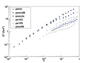
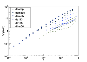
The main features of each experimental data set used in the present analysis are summarized in Tab. 1, and their kinematical coverage of the (x,Q2)𝑥superscript𝑄2(x,Q^{2})-plane is shown in Fig. 1. We observe that the kinematical coverage of the available data is rather small, especially when compared to the one of the available unpolarized DIS data, thus we will have a sizable region of the kinematical plane in which the fit extrapolates the behaviour extracted from the region covered by data.

From Tab. 1 we infer that the systematic errors are on average one order of magnitude smaller than the statistical ones. This justifies the procedure of neglecting correlations for systematic errors and the procedure of summing errors in quadrature when computing the figure of merit (χ2superscript𝜒2\chi^{2}) to be minimized in the fitting procedure.

Finally we notice that E155 data have been corrected to yield A1subscript𝐴1A_{1} by adding in Eq. (4) the g2subscript𝑔2g_{2} contribution evaluated with the Wandzura–Wilczek relation and using the parametrization of g1/F1subscript𝑔1subscript𝐹1g_{1}/F_{1} given in Ref. [14]: this shift is also added as a source of uncertainty in the total error of the data set.

Experiment x𝑥x range Q2(GeV2)superscript𝑄2superscriptGeV2Q^{2}(\mathrm{GeV}^{2}) range Ndatsubscript𝑁datN_{\rm dat} σstatdelimited-⟨⟩subscript𝜎stat\left\langle\sigma_{\mathrm{stat}}\right\rangle σsystdelimited-⟨⟩subscript𝜎syst\left\langle\sigma_{\mathrm{syst}}\right\rangle σnormdelimited-⟨⟩subscript𝜎norm\left\langle\sigma_{\mathrm{norm}}\right\rangle Type Ref.
Proton
EMC 0.015 - 0.466 3.5 - 29.5 10 0.077 0.024 0.028 A1subscript𝐴1A_{1} [10]
SMC 0.001 - 0.480 0.3 - 58.0 15 0.026 0.003 0.012 A1subscript𝐴1A_{1} [11]
SMC low-x𝑥x 0.0001 - 0.121 0.02 - 23.1 15 0.033 0.002 0.006 A1subscript𝐴1A_{1} [12]
E143 0.031 - 0.75 1.27 - 9.52 28 0.045 0.016 0.012 A1subscript𝐴1A_{1} [13]
E155 0.015 - 0.75 1.22 - 34.72 24 0.043 0.018 0.026 g1/F1subscript𝑔1subscript𝐹1g_{1}/F_{1} [14]
HERMES06 0.0058 - 0.7311 0.26 - 14.29 45 0.126 0.019 0.017 A1subscript𝐴1A_{1} [15]
Deuteron
COMPASS 0.0051 - 0.474 1.18 - 47.5 12 0.034 0.017 0.011 A1subscript𝐴1A_{1} [16]
SMC 0.001 - 0.480 0.3 - 58.0 15 0.032 0.003 0.006 A1subscript𝐴1A_{1} [11]
SMC low-x𝑥x 0.0001 - 0.121 0.02 - 23.1 15 0.069 0.005 0.005 A1subscript𝐴1A_{1} [12]
E143 0.031 - 0.75 1.27 - 9.52 28 0.066 0.011 0.008 A1subscript𝐴1A_{1} [13]
E155 0.015 - 0.75 1.22 - 34.72 24 0.091 0.009 0.011 g1/F1subscript𝑔1subscript𝐹1g_{1}/F_{1} [14]
HERMES06 0.0058 - 0.7311 0.26 - 14.29 45 0.089 0.007 0.009 A1subscript𝐴1A_{1} [15]
Table 1: The proton and deuteron experimental data sets included in the present analysis. We show the kinematic range, the number of points, the average statistical, systematic and normalization uncertainty, and the measured observable.
Refer to caption
Refer to caption
Figure 1: Experimental data in the (x,Q2)𝑥superscript𝑄2(x,Q^{2}) plane used in the present analysis for the proton (left) and for the deuteron (right) target.

3 The NNPDF approach

In this section we briefly review the approach used to extract an unbiased determination of the asymmetry A1subscript𝐴1A_{1} and the structure function g1subscript𝑔1g_{1} from the available inclusive polarized DIS data, following the analysis performed by the NNPDF Collaboration for the determination of the unpolarized structure function F2subscript𝐹2F_{2} [1, 2] and the parton densities [3, 4, 5].

The core idea underlying the NNPDF approach is based on using Monte Carlo methods to build a representation of the probability measure in the space of structure functions, and parametrizing the space of structure functions using neural networks. We refer the interested reader to the papers cited above for a detailed description of the methods and in the following we will briefly discuss the settings used in this analysis. It is worthwhile emphasizing that the Monte Carlo method does not require the use of neural networks, and would yield a robust determination of the errors with any parametrization of the structure function, provided the parametrization is sufficiently flexible. A comparison of Monte Carlo analyses based on different parametrizations was performed in the framework of the HERA-LHC workshop by comparing the standard H1 and NNPDF analyses. The greater flexibility of the neural network parametrization compared to fixed functional forms is reflected in the larger error bands obtained using the NNPDF method, especially when considering the x𝑥x region not covered by data (i.e.  the extrapolation region). These features are illustrated by the results in Sects. 3.2 and 3.4 of Ref. [17].

3.1 Monte-Carlo replicas

We generate Nrepsubscript𝑁repN_{\mathrm{rep}} Monte-Carlo replicas of the experimental data according to

A1(art),k(x,Q2)=(1+rk,NσNA1(exp)(x,Q2))[A1(exp)(x,Q2)+rk,tσt(x,Q2)],superscriptsubscript𝐴1art𝑘𝑥superscript𝑄21subscript𝑟𝑘𝑁subscript𝜎𝑁superscriptsubscript𝐴1exp𝑥superscript𝑄2delimited-[]superscriptsubscript𝐴1exp𝑥superscript𝑄2subscript𝑟𝑘𝑡subscript𝜎𝑡𝑥superscript𝑄2A_{1}^{(\mathrm{art}),k}(x,Q^{2})=\left(1+r_{k,N}\frac{\sigma_{N}}{A_{1}^{(\mathrm{exp})}(x,Q^{2})}\right)\Big{[}A_{1}^{(\mathrm{exp})}(x,Q^{2})+r_{k,t}\sigma_{t}(x,Q^{2})\Big{]}, (7)

where rksubscript𝑟𝑘r_{k} are Gaussian distributed random numbers, σNsubscript𝜎𝑁\sigma_{N} is the quadratic sum of the normalization errors and σtsubscript𝜎𝑡\sigma_{t} is the total error, obtained by summing in quadrature the statistical and systematic errors, the latter assumed to be uncorrelated.

Following Ref. [18], the covariance matrix for experimental data points is evaluated using:

covij=σNiσNj+δijσi,t,subscriptcov𝑖𝑗subscript𝜎subscript𝑁𝑖subscript𝜎subscript𝑁𝑗subscript𝛿𝑖𝑗subscript𝜎𝑖𝑡{\rm cov}_{ij}=\sigma_{N_{i}}\sigma_{N_{j}}+\delta_{ij}\sigma_{i,t}\,, (8)

while during the fit for each replica, we minimize:

χ2(k)=i=1Ndata(A1(art),k(x,Q2)A1(net),k(x,Q2)σ¯i,t(k)),superscript𝜒2𝑘superscriptsubscript𝑖1subscript𝑁datasuperscriptsubscript𝐴1𝑎𝑟𝑡𝑘𝑥superscript𝑄2superscriptsubscript𝐴1𝑛𝑒𝑡𝑘𝑥superscript𝑄2superscriptsubscript¯𝜎𝑖𝑡𝑘\chi^{2(k)}=\sum_{i=1}^{N_{\rm data}}\left(\frac{A_{1}^{(art),k}(x,Q^{2})-A_{1}^{(net),k}(x,Q^{2})}{\bar{\sigma}_{i,t}^{(k)}}\right)\,, (9)

where

σ¯i,t(k)=(1+rk,NσNA1(exp)(x,Q2))σi,t.superscriptsubscript¯𝜎𝑖𝑡𝑘1subscript𝑟𝑘𝑁subscript𝜎𝑁superscriptsubscript𝐴1𝑒𝑥𝑝𝑥superscript𝑄2subscript𝜎𝑖𝑡\bar{\sigma}_{i,t}^{(k)}=\left(1+r_{k,N}\frac{\sigma_{N}}{A_{1}^{(exp)}(x,Q^{2})}\right)\sigma_{i,t}\,. (10)

The number of Monte Carlo replicas of the data is determined by requiring that the average over the replicas reproduces the features (central values, errors and correlations) of the original experimental data to a required accuracy. The quantitative check is performed by means of the statistical estimators described in the appendix of Ref. [2] and the results for sets of 10, 100 and 1000 replicas are collected in Tab. 2 for the proton target data and in Tab. 3 for the deuteron target data. We observe that all the considered estimators have the correct scaling behaviour as the number of replica grows. We also point out that the large percentage error on the deuteron central values is due to a bulk of data whose values are close to zero.

10 100 1000
PE[A1(art)rep]delimited-⟨⟩𝑃𝐸delimited-[]subscriptdelimited-⟨⟩superscriptsubscript𝐴1𝑎𝑟𝑡rep\langle PE\left[\langle A_{1}^{(art)}\rangle_{\mathrm{rep}}\right]\rangle 14.20% 3.21% 1.83%
r[A1(art)]𝑟delimited-[]superscriptsubscript𝐴1𝑎𝑟𝑡r\left[A_{1}^{(art)}\right] 0.974203 0.998114 0.999682
V[σ(art)]datsubscriptdelimited-⟨⟩𝑉delimited-[]superscript𝜎𝑎𝑟𝑡dat\langle V\left[\sigma^{(art)}\right]\rangle_{\mathrm{dat}} 3.11033.1superscript1033.1\cdot 10^{-3} 1.51031.5superscript1031.5\cdot 10^{-3} 6.51046.5superscript1046.5\cdot 10^{-4}
PE[σ(art)]datsubscriptdelimited-⟨⟩𝑃𝐸delimited-[]delimited-⟨⟩superscript𝜎𝑎𝑟𝑡dat\langle PE\left[\langle\sigma^{(art)}\rangle\right]\rangle_{\mathrm{dat}} 35.45% 12.44% 4.20%
σ(art)datsubscriptdelimited-⟨⟩superscript𝜎𝑎𝑟𝑡dat\langle\sigma^{(art)}\rangle_{\mathrm{dat}} 0.0699 0.0766 0.0768
r[σ(art)]𝑟delimited-[]superscript𝜎𝑎𝑟𝑡r\left[\sigma^{(art)}\right] 0.989956 0.997808 0.999793
V[ρ(art)]datsubscriptdelimited-⟨⟩𝑉delimited-[]superscript𝜌𝑎𝑟𝑡dat\langle V\left[\rho^{(art)}\right]\rangle_{\mathrm{dat}} 9.51029.5superscript1029.5\cdot 10^{-2} 8.91038.9superscript1038.9\cdot 10^{-3} 9.21049.2superscript1049.2\cdot 10^{-4}
ρ(art)datsubscriptdelimited-⟨⟩superscript𝜌𝑎𝑟𝑡dat\langle\rho^{(art)}\rangle_{\mathrm{dat}} 0.1469 0.1567 0.1585
r[ρ(art)]𝑟delimited-[]superscript𝜌𝑎𝑟𝑡r\left[\rho^{(art)}\right] 0.638102 0.944682 0.993523
V[cov(art)]datsubscriptdelimited-⟨⟩𝑉delimited-[]superscriptcov𝑎𝑟𝑡dat\langle V\left[\mathrm{cov}^{(art)}\right]\rangle_{\mathrm{dat}} 7.61057.6superscript1057.6\cdot 10^{-5} 1.11051.1superscript1051.1\cdot 10^{-5} 1.51061.5superscript1061.5\cdot 10^{-6}
cov(art)datsubscriptdelimited-⟨⟩superscriptcov𝑎𝑟𝑡dat\langle\mathrm{cov}^{(art)}\rangle_{\mathrm{dat}} 0.00166 0.00154 0.00160
r[cov(art)]𝑟delimited-[]superscriptcov𝑎𝑟𝑡r\left[\mathrm{cov}^{(art)}\right] 0.898803 0.986219 0.998858
Table 2: Statistical estimators for Monte Carlo replicas of A1subscript𝐴1A_{1} for the proton data. The experimental data have σ(exp)dat=0.0764subscriptdelimited-⟨⟩superscript𝜎expdat0.0764\langle\sigma^{(\mathrm{exp})}\rangle_{\mathrm{dat}}=0.0764, ρ(exp)dat=0.1566subscriptdelimited-⟨⟩superscript𝜌expdat0.1566\langle\rho^{(\mathrm{exp})}\rangle_{\mathrm{dat}}=0.1566, and cov(exp)dat=0.00153subscriptdelimited-⟨⟩superscriptcovexpdat0.00153\langle\mathrm{cov}^{(\mathrm{exp})}\rangle_{\mathrm{dat}}=0.00153.
10 100 1000
PE[A1(art)rep]delimited-⟨⟩𝑃𝐸delimited-[]subscriptdelimited-⟨⟩superscriptsubscript𝐴1𝑎𝑟𝑡rep\langle PE\left[\langle A_{1}^{(art)}\rangle_{\mathrm{rep}}\right]\rangle 89.71% 24.90% 5.97%
r[A1(art)]𝑟delimited-[]superscriptsubscript𝐴1𝑎𝑟𝑡r\left[A_{1}^{(art)}\right] 0.977524 0.98633 0.999865
V[σ(art)]datsubscriptdelimited-⟨⟩𝑉delimited-[]superscript𝜎𝑎𝑟𝑡dat\langle V\left[\sigma^{(art)}\right]\rangle_{\mathrm{dat}} 5.31035.3superscript1035.3\cdot 10^{-3} 1.71031.7superscript1031.7\cdot 10^{-3} 6.71046.7superscript1046.7\cdot 10^{-4}
PE[σ(art)]datsubscriptdelimited-⟨⟩𝑃𝐸delimited-[]delimited-⟨⟩superscript𝜎𝑎𝑟𝑡dat\langle PE\left[\langle\sigma^{(art)}\rangle\right]\rangle_{\mathrm{dat}} 35.03% 11.75% 4.4%
σ(art)datsubscriptdelimited-⟨⟩superscript𝜎𝑎𝑟𝑡dat\langle\sigma^{(art)}\rangle_{\mathrm{dat}} 0.0689 0.0739 0.0734
r[σ(art)]𝑟delimited-[]superscript𝜎𝑎𝑟𝑡r\left[\sigma^{(art)}\right] 0.977501 0.997965 0.999705
V[ρ(art)]datsubscriptdelimited-⟨⟩𝑉delimited-[]superscript𝜌𝑎𝑟𝑡dat\langle V\left[\rho^{(art)}\right]\rangle_{\mathrm{dat}} 1.01021.0superscript1021.0\cdot 10^{-2} 9.21039.2superscript1039.2\cdot 10^{-3} 8.71048.7superscript1048.7\cdot 10^{-4}
ρ(art)datsubscriptdelimited-⟨⟩superscript𝜌𝑎𝑟𝑡dat\langle\rho^{(art)}\rangle_{\mathrm{dat}} 0.0878 0.0904 0.0861
r[ρ(art)]𝑟delimited-[]superscript𝜌𝑎𝑟𝑡r\left[\rho^{(art)}\right] 0.612155 0.932158 0.992952
V[cov(art)]datsubscriptdelimited-⟨⟩𝑉delimited-[]superscriptcov𝑎𝑟𝑡dat\langle V\left[\mathrm{cov}^{(art)}\right]\rangle_{\mathrm{dat}} 6.31056.3superscript1056.3\cdot 10^{-5} 1.01051.0superscript1051.0\cdot 10^{-5} 1.01061.0superscript1061.0\cdot 10^{-6}
cov(art)datsubscriptdelimited-⟨⟩superscriptcov𝑎𝑟𝑡dat\langle\mathrm{cov}^{(art)}\rangle_{\mathrm{dat}} 0.00133 0.00145 0.00134
r[cov(art)]𝑟delimited-[]superscriptcov𝑎𝑟𝑡r\left[\mathrm{cov}^{(art)}\right] 0.959275 0.995339 0.999479
Table 3: Statistical estimators for Monte Carlo replicas of A1subscript𝐴1A_{1} for the deuteron data. The experimental data have σ(exp)dat=0.0733subscriptdelimited-⟨⟩superscript𝜎expdat0.0733\langle\sigma^{(\mathrm{exp})}\rangle_{\mathrm{dat}}=0.0733, ρ(exp)dat=0.0862subscriptdelimited-⟨⟩superscript𝜌expdat0.0862\langle\rho^{(\mathrm{exp})}\rangle_{\mathrm{dat}}=0.0862, and cov(exp)dat=0.00135subscriptdelimited-⟨⟩superscriptcovexpdat0.00135\langle\mathrm{cov}^{(\mathrm{exp})}\rangle_{\mathrm{dat}}=0.00135.

3.2 Neural Networks as unbiased interpolants

Artificial neural networks, see e.g. Ref. [19], are a class of algorithms which provide a robust and universal approximant to incomplete or noisy data, with the only requirement of continuity. Neural networks are universal approximators for measurable functions [20]. This means that any continuous function can be approximated to any degree of accuracy by a sufficiently large neural network with one hidden layer and non-linear neuron activation function.

One of the main reasons to use neural networks in place of any other redundant parametrization is the existence of efficient techniques for training them, i.e. determining the parameters of the network (thresholds and weights) so that it reproduces a given set of input-output data. Equivalently one could say that a sufficiently large neural network provides a description of the data which is largely free of functional bias.

The analysis presented here uses a class of neural networks known as multilayer feed-forward perceptrons, trained using a genetic algorithm [21, 22]. The networks we employed have one hidden layer and a 2-4-1 architecture, which gives us a total of 17 free parameters for each network to be determined during the training. The guidance principle in the choice of the network architecture to be used is that it should provide a redundant parametrization for the data to be fitted, i.e. the network should have enough flexibility to fit not only the underlying physical law but also the statistical fluctuations of the experimental data. This property is crucial in ensuring that the fit results are not biased by the specific parametrization. The lack of functional bias is established a posteriori by verifying that fits performed with networks with different architectures lead to statistically equivalent results. This is achieved using the statistical estimators introduced in the NNPDF Collaboration’s studies; the results of these comparisons are presented and discussed later.
Refer to caption
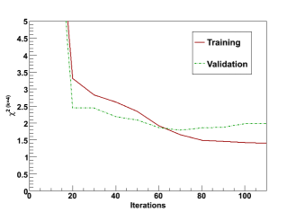
Figure 2: χ2superscript𝜒2\chi^{2} for the training (red) and validation (green) sets of one replica in the reference fit to A1psuperscriptsubscript𝐴1𝑝A_{1}^{p}.

The training of the individual networks to the Monte Carlo replicas is performed by minimizing the figure of merit given in Eq. (9). Given the extensive size and complex structure of the parameter space (a neural network with n𝑛n parameters, weights and thresholds has 2n!2𝑛2n! equivalent global minimum configurations), the most efficient training algorithm turns out to be a genetic algorithm. The details of the implementation are discussed in Ref. [3].

As already pointed out in various references the fact that we adopt a redundant parametrization and that the figure of merit minimized in the training procedure is monotonically decreasing might lead to overfitting the data: the neural network reproduces not only the underlying physical law but also the statistical noise of the data sample. To prevent this from happening and to determine the optimal fit we adopt a criterion to stop our fit based on the cross-validation method. Once again our procedure is completely analogous to the one used for the unpolarized NNPDF fits.

For each replica of the experimental data we subdivide the data into a training and a validation set, respectively containing a fraction ftrsubscript𝑓trf_{\mathrm{tr}} and (1ftr)1subscript𝑓tr(1-f_{\mathrm{tr}}) of randomly chosen data points of each experiment.

We train one neural network on each replica of the data using the χ2superscript𝜒2\chi^{2} of the training set as a figure of merit to be minimized. In parallel we compute the χ2superscript𝜒2\chi^{2} of the validation set. We stop the training when we find that the χ2superscript𝜒2\chi^{2} smeared over a given number of generations is decreasing for the training set while increasing for the validation set. A graphical illustration of such a behaviour for one of the replicas in the reference fit is given in Fig. 2.

4 Phenomenology

The study of the first moments of polarized structure functions is of phenomenological interest, since they can be used to extract information on the fraction of polarization carried by partons and on physical couplings. In the MS¯¯MS\overline{\mathrm{MS}} scheme we have

Γ1p,n(Q2)superscriptsubscriptΓ1𝑝𝑛superscript𝑄2\displaystyle\Gamma_{1}^{p,n}(Q^{2}) =\displaystyle= 01𝑑xg1p,n(x,Q2)=superscriptsubscript01differential-d𝑥superscriptsubscript𝑔1𝑝𝑛𝑥superscript𝑄2absent\displaystyle\int_{0}^{1}dx\,g_{1}^{p,n}(x,Q^{2})=
=\displaystyle= 136[(a8±3a3)ΔCNSMS¯(αs(Q2))+4a0ΔCSMS¯(αs(Q2))],136delimited-[]plus-or-minussubscript𝑎83subscript𝑎3Δsuperscriptsubscript𝐶NS¯MSsubscript𝛼𝑠superscript𝑄24subscript𝑎0Δsuperscriptsubscript𝐶S¯MSsubscript𝛼𝑠superscript𝑄2\displaystyle\frac{1}{36}\left[(a_{8}\pm 3a_{3})\Delta C_{\mathrm{NS}}^{\overline{\mathrm{MS}}}(\alpha_{s}(Q^{2}))+4a_{0}\Delta C_{\mathrm{S}}^{\overline{\mathrm{MS}}}(\alpha_{s}(Q^{2}))\right]\,,

where ΔCNSMS¯(αs(Q2))Δsuperscriptsubscript𝐶NS¯MSsubscript𝛼𝑠superscript𝑄2\Delta C_{\mathrm{NS}}^{\overline{\mathrm{MS}}}(\alpha_{s}(Q^{2})) and ΔCSMS¯(αs(Q2))Δsuperscriptsubscript𝐶S¯MSsubscript𝛼𝑠superscript𝑄2\Delta C_{\mathrm{S}}^{\overline{\mathrm{MS}}}(\alpha_{s}(Q^{2})) are the first moments of the non-singlet and singlet Wilson coefficient functions, respectively, and

a3subscript𝑎3\displaystyle a_{3} =\displaystyle= (Δu+Δu¯)(Δd+Δd¯),Δ𝑢Δ¯𝑢Δ𝑑Δ¯𝑑\displaystyle(\Delta u+\Delta\bar{u})-(\Delta d+\Delta\bar{d})\,, (12)
a8subscript𝑎8\displaystyle a_{8} =\displaystyle= (Δu+Δu¯)+(Δd+Δd¯)2(Δs+Δs¯),Δ𝑢Δ¯𝑢Δ𝑑Δ¯𝑑2Δ𝑠Δ¯𝑠\displaystyle(\Delta u+\Delta\bar{u})+(\Delta d+\Delta\bar{d})-2(\Delta s+\Delta\bar{s})\,, (13)
a0subscript𝑎0\displaystyle a_{0} =\displaystyle= (Δu+Δu¯)+(Δd+Δd¯)+(Δs+Δs¯)ΔΣ.Δ𝑢Δ¯𝑢Δ𝑑Δ¯𝑑Δ𝑠Δ¯𝑠ΔΣ\displaystyle(\Delta u+\Delta\bar{u})+(\Delta d+\Delta\bar{d})+(\Delta s+\Delta\bar{s})\equiv\Delta\Sigma\,. (14)

Using isotopic spin invariance, it can be shown that a3subscript𝑎3a_{3} is the axial coupling gA=GA/GVsubscript𝑔𝐴subscript𝐺𝐴subscript𝐺𝑉g_{A}=G_{A}/G_{V} that governs neutron β𝛽\beta-decay. Accurate measurements yield (see e.g. Ref. [9]):

gA=1.2670±0.0035.subscript𝑔𝐴plus-or-minus1.26700.0035g_{A}=1.2670\pm 0.0035\,. (15)

The difference of the g1subscript𝑔1g_{1} moments for proton and neutron leads to the Bjorken sum rule

Γ1NS(Q2)=Γ1p(Q2)Γ1n(Q2)=16gAΔCNSMS¯(αs(Q2))+δT+δτ;superscriptsubscriptΓ1NSsuperscript𝑄2superscriptsubscriptΓ1𝑝superscript𝑄2superscriptsubscriptΓ1𝑛superscript𝑄216subscript𝑔𝐴Δsuperscriptsubscript𝐶NS¯MSsubscript𝛼𝑠superscript𝑄2subscript𝛿𝑇subscript𝛿𝜏\Gamma_{1}^{\mathrm{NS}}(Q^{2})=\Gamma_{1}^{p}(Q^{2})-\Gamma_{1}^{n}(Q^{2})=\frac{1}{6}g_{A}\Delta C_{\mathrm{NS}}^{\overline{\mathrm{MS}}}(\alpha_{s}(Q^{2}))+\delta_{T}+\delta_{\tau}\,; (16)

where δTsubscript𝛿𝑇\delta_{T} is the target mass correction and δtsubscript𝛿𝑡\delta_{t} is the correction due to higher twists. Target mass corrections have been studied in Refs. [23, 24, 25, 26] and can be evaluated for any moment n𝑛n at the first order in m2/Q2superscript𝑚2superscript𝑄2m^{2}/Q^{2} using [24]:

δT=g1(n)(Q2)g10(n)(Q2)=m2Q2n(n+1)(n+2)2[(n+4)g10n+2(Q2)+4n+2n+1g20n+2(Q2)],subscript𝛿𝑇superscriptsubscript𝑔1𝑛superscript𝑄2superscriptsubscript𝑔10𝑛superscript𝑄2superscript𝑚2superscript𝑄2𝑛𝑛1superscript𝑛22delimited-[]𝑛4superscriptsubscript𝑔10𝑛2superscript𝑄24𝑛2𝑛1superscriptsubscript𝑔20𝑛2superscript𝑄2\delta_{T}=g_{1}^{(n)}(Q^{2})-g_{10}^{(n)}(Q^{2})=\frac{m^{2}}{Q^{2}}\frac{n(n+1)}{(n+2)^{2}}\left[(n+4)g_{10}^{n+2}(Q^{2})+4\frac{n+2}{n+1}g_{20}^{n+2}(Q^{2})\right]\,, (17)

where gi(n)(Q2)=01𝑑xxn1gi(x,Q2)superscriptsubscript𝑔𝑖𝑛superscript𝑄2superscriptsubscript01differential-d𝑥superscript𝑥𝑛1subscript𝑔𝑖𝑥superscript𝑄2g_{i}^{(n)}(Q^{2})=\int_{0}^{1}dx\,x^{n-1}g_{i}(x,Q^{2}) and gi0subscript𝑔𝑖0g_{i0} is the structure function taken at zero mass of the nucleon. The higher–twist contribution is simply

δτ=μ4Q2,subscript𝛿𝜏subscript𝜇4superscript𝑄2\delta_{\tau}=\frac{\mu_{4}}{Q^{2}}\,, (18)

where μ4subscript𝜇4\mu_{4} can be extracted from experimental data at low Q2superscript𝑄2Q^{2} such as the CLAS data [27]. Finally, the coefficient function of Eq. (16) has been calculated in Ref. [28] and up to order αs3superscriptsubscript𝛼𝑠3\alpha_{s}^{3} is given by:

ΔCNSMS¯(αs(Q2))Δsuperscriptsubscript𝐶NS¯MSsubscript𝛼𝑠superscript𝑄2\displaystyle\Delta C_{\mathrm{NS}}^{\overline{\mathrm{MS}}}(\alpha_{s}(Q^{2})) =\displaystyle= 1αs(Q2)π(5512nf3)(αs(Q2)π)21subscript𝛼𝑠superscript𝑄2𝜋5512subscript𝑛𝑓3superscriptsubscript𝛼𝑠superscript𝑄2𝜋2\displaystyle 1-\frac{\alpha_{s}(Q^{2})}{\pi}-\left(\frac{55}{12}-\frac{n_{f}}{3}\right)\left(\frac{\alpha_{s}(Q^{2})}{\pi}\right)^{2} (19)
\displaystyle- (41.43997.6072nf+115648nf2)(αs(Q2)π)3.41.43997.6072subscript𝑛𝑓115648superscriptsubscript𝑛𝑓2superscriptsubscript𝛼𝑠superscript𝑄2𝜋3\displaystyle\left(41.4399-7.6072\,n_{f}+\frac{115}{648}\,n_{f}^{2}\right)\left(\frac{\alpha_{s}(Q^{2})}{\pi}\right)^{3}\,.

For the running coupling we use the expanded solution of the renormalization group equation, up to NNLO we have:

αs(Q2)subscript𝛼𝑠superscript𝑄2\displaystyle\alpha_{s}\left(Q^{2}\right) =\displaystyle= αs(Q2)LO[1+αs(Q2)LO[αs(Q2)LOαs(MZ2)](b2b12)\displaystyle\alpha_{s}\left(Q^{2}\right)_{\mathrm{LO}}\Bigg{[}1+\alpha_{s}\left(Q^{2}\right)_{\mathrm{LO}}\left[\alpha_{s}\left(Q^{2}\right)_{\mathrm{LO}}-\alpha_{s}\left(M_{Z}^{2}\right)\right](b_{2}-b_{1}^{2}) (20)
+\displaystyle+ αs(Q2)NLOb1lnαs(Q2)NLOαs(MZ2)],\displaystyle\alpha_{s}\left(Q^{2}\right)_{\mathrm{NLO}}b_{1}\ln\frac{\alpha_{s}\left(Q^{2}\right)_{\mathrm{NLO}}}{\alpha_{s}\left(M_{Z}^{2}\right)}\Bigg{]},

with

αs(Q2)NLO=αs(Q2)LO[1b1αs(Q2)LOln(1+β0αs(MZ2)lnQ2MZ2)],subscript𝛼𝑠subscriptsuperscript𝑄2NLOsubscript𝛼𝑠subscriptsuperscript𝑄2LOdelimited-[]1subscript𝑏1subscript𝛼𝑠subscriptsuperscript𝑄2LO1subscript𝛽0subscript𝛼𝑠superscriptsubscript𝑀𝑍2superscript𝑄2superscriptsubscript𝑀𝑍2\displaystyle\alpha_{s}\left(Q^{2}\right)_{\mathrm{NLO}}=\alpha_{s}\left(Q^{2}\right)_{\mathrm{LO}}\left[1-b_{1}\alpha_{s}\left(Q^{2}\right)_{\mathrm{LO}}\ln\left(1+\beta_{0}\alpha_{s}\left(M_{Z}^{2}\right)\ln\frac{Q^{2}}{M_{Z}^{2}}\right)\right]\ , (21)
αs(Q2)LO=αs(MZ2)1+β0αs(MZ2)lnQ2MZ2,subscript𝛼𝑠subscriptsuperscript𝑄2LOsubscript𝛼𝑠superscriptsubscript𝑀𝑍21subscript𝛽0subscript𝛼𝑠superscriptsubscript𝑀𝑍2superscript𝑄2superscriptsubscript𝑀𝑍2\displaystyle\alpha_{s}\left(Q^{2}\right)_{\mathrm{LO}}=\frac{\alpha_{s}\left(M_{Z}^{2}\right)}{1+\beta_{0}\alpha_{s}\left(M_{Z}^{2}\right)\ln\frac{Q^{2}}{M_{Z}^{2}}}, (22)

and the beta function coefficients given by

Q2das(Q2)dQ2=k=02βkas(Q2)k+2,as(Q2)=αs(Q2)4π,formulae-sequencesuperscript𝑄2𝑑subscript𝑎𝑠superscript𝑄2𝑑superscript𝑄2superscriptsubscript𝑘02subscript𝛽𝑘subscript𝑎𝑠superscriptsuperscript𝑄2𝑘2subscript𝑎𝑠superscript𝑄2subscript𝛼𝑠superscript𝑄24𝜋\displaystyle Q^{2}\frac{da_{s}(Q^{2})}{dQ^{2}}=-\sum_{k=0}^{2}\beta_{k}a_{s}(Q^{2})^{k+2},\qquad a_{s}(Q^{2})=\frac{\alpha_{s}(Q^{2})}{4\pi}\,, (23)

where

β0subscript𝛽0\displaystyle\beta_{0} =\displaystyle= 1123nf,1123subscript𝑛𝑓\displaystyle 11-\frac{2}{3}n_{f}\ , (24)
β1subscript𝛽1\displaystyle\beta_{1} =\displaystyle= 102383nf,102383subscript𝑛𝑓\displaystyle 102-\frac{38}{3}n_{f}\ ,
β2subscript𝛽2\displaystyle\beta_{2} =\displaystyle= 28572503318nf+32554nf2,28572503318subscript𝑛𝑓32554superscriptsubscript𝑛𝑓2\displaystyle\frac{2857}{2}-\frac{5033}{18}n_{f}+\frac{325}{54}n_{f}^{2}\,,

and biβi/β0subscript𝑏𝑖subscript𝛽𝑖subscript𝛽0b_{i}\equiv\beta_{i}/\beta_{0}.

5 Results

In this section we present our parametrization of the proton and deuteron asymmetries and the structure functions extracted from them.

We assess the quality of the fit by comparing our extraction with the experimental data included in the analysis, and by studying the stability of our results under variations of the parametrization used for the networks.

Then, as an example of a possible application of our result to a phenomenological analysis, we study the extraction of the physical parameters (the strong coupling constant αssubscript𝛼𝑠\alpha_{s} and the axial coupling gAsubscript𝑔𝐴g_{A}) from the Bjorken sum rule. In order to give a faithful error on the extracted quantities we study the impact of the different assumptions which are needed to reconstruct the structure functions and then to evaluate the Bjorken sum rule. Results are compared to existing estimates.

5.1 The final fit and its statistical features

Proton χ2superscript𝜒2\chi^{2} Deuteron χ2superscript𝜒2\chi^{2}
EMC 0.370 COMPASS 0.885
SMC 0.480 SMC 1.100
SMC low-x𝑥x 1.150 SMC low-x𝑥x 0.774
E143 0.904 E143 1.530
E155 0.717 E155 0.661
HERMES06 0.456 HERMES06 0.881
Total 0.666 Total 0.986
Table 4: The χ2superscript𝜒2\chi^{2} of the fit for proton and deuteron data.

In Tab. 4 we show the χ2/Ndatasuperscript𝜒2subscript𝑁data\chi^{2}/N_{\mathrm{data}} for each target and each experimental data set included in the present analysis. We first observe the overall good quality of our fit. For the proton the small values of χ2superscript𝜒2\chi^{2} for EMC, SMC and HERMES can be explained by a possible overestimate of experimental errors. For the deuteron all the χ2superscript𝜒2\chi^{2} are of order 1, except for the E155 data set which has a value of χ2superscript𝜒2\chi^{2} significantly smaller than one. The somewhat larger value of χ2superscript𝜒2\chi^{2} for the E143 deuteron data set can be understood by looking at Figs. 3 and 4 where we present a comparison of our fit to experimental data in different kinematical regions. We observe that in the case of E143 the deuteron data show small incompatibilities among themselves, and the large value of χ2superscript𝜒2\chi^{2} is a reflection of this. It is interesting to remark that a careful analysis of the χ2superscript𝜒2\chi^{2} value for each experiment allows the identification of potential incompatible data. This feature had already been pointed out in the unpolarized studies by the NNPDF Collaboration.
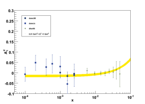
Refer to caption
Refer to caption
Refer to caption
Refer to caption
Refer to caption
Refer to caption
Figure 3: The fitted asymmetries compared to proton (left) and deuteron (right) data for 0.01GeV2<Q2<1GeV20.01superscriptGeV2superscript𝑄21superscriptGeV20.01\leavevmode\nobreak\ \mathrm{GeV}^{2}<Q^{2}<1\leavevmode\nobreak\ \mathrm{GeV}^{2} (upper row), 1GeV2<Q2<3GeV21superscriptGeV2superscript𝑄23superscriptGeV21\leavevmode\nobreak\ \mathrm{GeV}^{2}<Q^{2}<3\leavevmode\nobreak\ \mathrm{GeV}^{2} (central row) and 3GeV2<Q2<5GeV23superscriptGeV2superscript𝑄25superscriptGeV23\leavevmode\nobreak\ \mathrm{GeV}^{2}<Q^{2}<5\leavevmode\nobreak\ \mathrm{GeV}^{2} (lower row). In the plots A1subscript𝐴1A_{1} is evaluated at the central value of each Q2superscript𝑄2Q^{2} range.
Refer to caption
Refer to caption
Refer to caption
Refer to caption
Refer to caption
Refer to caption
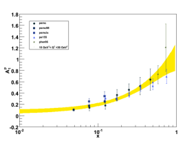
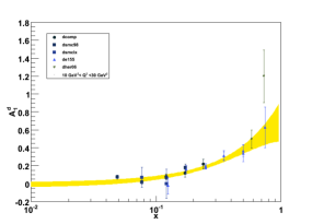
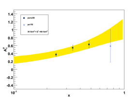
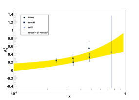
Figure 4: The fit compared to proton (left) and deuteron (right) data for 5GeV2<Q2<10GeV25superscriptGeV2superscript𝑄210superscriptGeV25\leavevmode\nobreak\ \mathrm{GeV}^{2}<Q^{2}<10\leavevmode\nobreak\ \mathrm{GeV}^{2} (upper row), 10GeV2<Q2<30GeV210superscriptGeV2superscript𝑄230superscriptGeV210\leavevmode\nobreak\ \mathrm{GeV}^{2}<Q^{2}<30\leavevmode\nobreak\ \mathrm{GeV}^{2} (central row) and 30GeV2<Q2<60GeV230superscriptGeV2superscript𝑄260superscriptGeV230\leavevmode\nobreak\ \mathrm{GeV}^{2}<Q^{2}<60\leavevmode\nobreak\ \mathrm{GeV}^{2} (lower row). In the plots A1subscript𝐴1A_{1} is evaluated at the central value of each Q2superscript𝑄2Q^{2} range.

In Tabs. 5, 6, and 7 we study the self–stability of the fit and the stability against the variation of the parametrization with respect to a smaller and a larger architecture. To this extent we define four different regions: one where we expect our fit to be an interpolation of the available data (Data region) and three where its behaviour is extrapolated to regions of the (x,Q2)𝑥superscript𝑄2(x,Q^{2})-plane not covered by present data:

  • Data: 0.01<x<0.750.01𝑥0.750.01<x<0.75 and 2GeV2<Q2<20GeV22superscriptGeV2superscript𝑄220superscriptGeV22\leavevmode\nobreak\ \mathrm{GeV}^{2}<Q^{2}<20\leavevmode\nobreak\ \mathrm{GeV}^{2};

  • Low-x𝑥x: 0.0001<x<0.0010.0001𝑥0.0010.0001<x<0.001 and 2GeV2<Q2<20GeV22superscriptGeV2superscript𝑄220superscriptGeV22\leavevmode\nobreak\ \mathrm{GeV}^{2}<Q^{2}<20\leavevmode\nobreak\ \mathrm{GeV}^{2};

  • Low-Q2superscript𝑄2Q^{2}: 0.2<x<0.80.2𝑥0.80.2<x<0.8 and 0.1GeV2<Q2<2GeV20.1superscriptGeV2superscript𝑄22superscriptGeV20.1\leavevmode\nobreak\ \mathrm{GeV}^{2}<Q^{2}<2\leavevmode\nobreak\ \mathrm{GeV}^{2};

  • High-Q2superscript𝑄2Q^{2}: 0.2<x<0.80.2𝑥0.80.2<x<0.8 and 20GeV2<Q2<60GeV220superscriptGeV2superscript𝑄260superscriptGeV220\leavevmode\nobreak\ \mathrm{GeV}^{2}<Q^{2}<60\leavevmode\nobreak\ \mathrm{GeV}^{2}.

We observe that all the estimators for self–stabilities are of order unity (or smaller), meaning that different subsets within the whole ensemble of replicas have the same statistical features.

When we compare our final fit to a fit performed using networks with a smaller architecture, we notice that the the two fits are statistically equivalent. The same happens for the comparison with a fit done with networks with a larger architecture, with the only exception of the errors on the deuteron fit in the extrapolation (all distances are order 1.5), which show some minor instability.

Proton Data Low-x𝑥x Low-Q2superscript𝑄2Q^{2} High-Q2superscript𝑄2Q^{2}
d[A1]delimited-⟨⟩𝑑delimited-[]subscript𝐴1\left\langle d[A_{1}]\right\rangle 0.963±0.011plus-or-minus0.9630.0110.963\pm 0.011 0.660±0.011plus-or-minus0.6600.0110.660\pm 0.011 1.085±0.015plus-or-minus1.0850.0151.085\pm 0.015 0.966±0.014plus-or-minus0.9660.0140.966\pm 0.014
d[σA1]delimited-⟨⟩𝑑delimited-[]subscript𝜎subscript𝐴1\left\langle d[\sigma_{A_{1}}]\right\rangle 0.840±0.006plus-or-minus0.8400.0060.840\pm 0.006 0.618±0.011plus-or-minus0.6180.0110.618\pm 0.011 0.966±0.014plus-or-minus0.9660.0140.966\pm 0.014 0.905±0.012plus-or-minus0.9050.0120.905\pm 0.012
Deuteron Data Low-x𝑥x Low-Q2superscript𝑄2Q^{2} High-Q2superscript𝑄2Q^{2}
d[A1]delimited-⟨⟩𝑑delimited-[]subscript𝐴1\left\langle d[A_{1}]\right\rangle 0.772±0.008plus-or-minus0.7720.0080.772\pm 0.008 0.670±0.012plus-or-minus0.6700.0120.670\pm 0.012 0.804±0.012plus-or-minus0.8040.0120.804\pm 0.012 0.688±0.011plus-or-minus0.6880.0110.688\pm 0.011
d[σA1]delimited-⟨⟩𝑑delimited-[]subscript𝜎subscript𝐴1\left\langle d[\sigma_{A_{1}}]\right\rangle 0.818±0.007plus-or-minus0.8180.0070.818\pm 0.007 0.899±0.014plus-or-minus0.8990.0140.899\pm 0.014 0.730±0.011plus-or-minus0.7300.0110.730\pm 0.011 0.773±0.011plus-or-minus0.7730.0110.773\pm 0.011
Table 5: Self–stability estimators evaluated with 100 replicas. The entries in the table show the statistical differences between results based on different subsets of 100 replicas randomly chosen in our Monte Carlo ensemble.
Proton Data Low-x𝑥x Low-Q2superscript𝑄2Q^{2} High-Q2superscript𝑄2Q^{2}
d[A1]delimited-⟨⟩𝑑delimited-[]subscript𝐴1\left\langle d[A_{1}]\right\rangle 0.952±0.010plus-or-minus0.9520.0100.952\pm 0.010 0.792±0.014plus-or-minus0.7920.0140.792\pm 0.014 0.859±0.012plus-or-minus0.8590.0120.859\pm 0.012 1.295±0.016plus-or-minus1.2950.0161.295\pm 0.016
d[σA1]delimited-⟨⟩𝑑delimited-[]subscript𝜎subscript𝐴1\left\langle d[\sigma_{A_{1}}]\right\rangle 1.104±0.008plus-or-minus1.1040.0081.104\pm 0.008 1.405±0.013plus-or-minus1.4050.0131.405\pm 0.013 0.975±0.014plus-or-minus0.9750.0140.975\pm 0.014 1.002±0.011plus-or-minus1.0020.0111.002\pm 0.011
Deuteron Data Low-x𝑥x Low-Q2superscript𝑄2Q^{2} High-Q2superscript𝑄2Q^{2}
d[A1]delimited-⟨⟩𝑑delimited-[]subscript𝐴1\left\langle d[A_{1}]\right\rangle 1.217±0.012plus-or-minus1.2170.0121.217\pm 0.012 1.302±0.012plus-or-minus1.3020.0121.302\pm 0.012 1.324±0.017plus-or-minus1.3240.0171.324\pm 0.017 0.703±0.010plus-or-minus0.7030.0100.703\pm 0.010
d[σA1]delimited-⟨⟩𝑑delimited-[]subscript𝜎subscript𝐴1\left\langle d[\sigma_{A_{1}}]\right\rangle 0.963±0.008plus-or-minus0.9630.0080.963\pm 0.008 1.199±0.010plus-or-minus1.1990.0101.199\pm 0.010 0.962±0.010plus-or-minus0.9620.0100.962\pm 0.010 1.689±0.019plus-or-minus1.6890.0191.689\pm 0.019
Table 6: Stability estimators for the reference fit (architecture 2-4-1) compared to a fit with a smaller architecture (2-3-1).
Proton Data Low-x𝑥x Low-Q2superscript𝑄2Q^{2} High-Q2superscript𝑄2Q^{2}
d[A1]delimited-⟨⟩𝑑delimited-[]subscript𝐴1\left\langle d[A_{1}]\right\rangle 1.076±0.012plus-or-minus1.0760.0121.076\pm 0.012 1.179±0.017plus-or-minus1.1790.0171.179\pm 0.017 0.693±0.011plus-or-minus0.6930.0110.693\pm 0.011 1.625±0.018plus-or-minus1.6250.0181.625\pm 0.018
d[σA1]delimited-⟨⟩𝑑delimited-[]subscript𝜎subscript𝐴1\left\langle d[\sigma_{A_{1}}]\right\rangle 1.258±0.010plus-or-minus1.2580.0101.258\pm 0.010 1.354±0.014plus-or-minus1.3540.0141.354\pm 0.014 0.709±0.010plus-or-minus0.7090.0100.709\pm 0.010 1.151±0.016plus-or-minus1.1510.0161.151\pm 0.016
Deuteron Data Low-x𝑥x Low-Q2superscript𝑄2Q^{2} High-Q2superscript𝑄2Q^{2}
d[A1]delimited-⟨⟩𝑑delimited-[]subscript𝐴1\left\langle d[A_{1}]\right\rangle 0.867±0.009plus-or-minus0.8670.0090.867\pm 0.009 0.794±0.012plus-or-minus0.7940.0120.794\pm 0.012 0.856±0.015plus-or-minus0.8560.0150.856\pm 0.015 0.840±0.017plus-or-minus0.8400.0170.840\pm 0.017
d[σA1]delimited-⟨⟩𝑑delimited-[]subscript𝜎subscript𝐴1\left\langle d[\sigma_{A_{1}}]\right\rangle 1.460±0.009plus-or-minus1.4600.0091.460\pm 0.009 1.941±0.015plus-or-minus1.9410.0151.941\pm 0.015 1.410±0.011plus-or-minus1.4100.0111.410\pm 0.011 1.303±0.011plus-or-minus1.3030.0111.303\pm 0.011
Table 7: Stability estimators for the reference fit (architecture 2-4-1) compared to a fit with a larger architecture (2-5-1).

5.2 Structure functions reconstruction

In order to reconstruct the structure function g1subscript𝑔1g_{1} from data on the asymmetry A1subscript𝐴1A_{1} as given in Eq. (4) some additional assumptions are needed. In the following we assess the impact of our assumptions for g2subscript𝑔2g_{2}, F2subscript𝐹2F_{2} and R𝑅R on the determination of first moment of g1subscript𝑔1g_{1}. These checks are done using an ensemble of 100 replicas, which is enough to this purpose, and in a range of x𝑥x and Q2superscript𝑄2Q^{2} which is entirely in the data region in order to avoid any extrapolation effects. Finally, we compare our result for 1000 replicas with the sum rules obtained by experimental collaborations.

The first assumption whose impact we consider is the one on the structure function g2subscript𝑔2g_{2}, which is evaluated from the Wandzura–Wilczek relation [29]

g2WW(x,Q2)=g1(x,Q2)+x1dyyg1(y,Q2).superscriptsubscript𝑔2𝑊𝑊𝑥superscript𝑄2subscript𝑔1𝑥superscript𝑄2superscriptsubscript𝑥1𝑑𝑦𝑦subscript𝑔1𝑦superscript𝑄2\displaystyle g_{2}^{WW}(x,Q^{2})=-g_{1}(x,Q^{2})+\int_{x}^{1}\frac{dy}{y}g_{1}(y,Q^{2})\,. (25)

Inserting this expression into Eq. (4) gives

g1(x,Q2)=11+γ2(A1(x,Q2)F1(x,Q2)+γ2x1dyyg1(y,Q2)),subscript𝑔1𝑥superscript𝑄211superscript𝛾2subscript𝐴1𝑥superscript𝑄2subscript𝐹1𝑥superscript𝑄2superscript𝛾2superscriptsubscript𝑥1𝑑𝑦𝑦subscript𝑔1𝑦superscript𝑄2\displaystyle g_{1}(x,Q^{2})=\frac{1}{1+\gamma^{2}}\left(A_{1}(x,Q^{2})F_{1}(x,Q^{2})+\gamma^{2}\int_{x}^{1}\frac{dy}{y}g_{1}(y,Q^{2})\right)\,, (26)

which needs to be evaluated iteratively. To this purpose we take the initial value g1(x,Q2)subscript𝑔1𝑥superscript𝑄2g_{1}(x,Q^{2}) evaluated with g2(x,Q2)=0subscript𝑔2𝑥superscript𝑄20g_{2}(x,Q^{2})=0, and we use

g1(iWW)(x,Q2)=11+γ2(A1(x,Q2)F1(x,Q2)+γ2x1dyyg1(iWW1)(y,Q2)).superscriptsubscript𝑔1subscript𝑖𝑊𝑊𝑥superscript𝑄211superscript𝛾2subscript𝐴1𝑥superscript𝑄2subscript𝐹1𝑥superscript𝑄2superscript𝛾2superscriptsubscript𝑥1𝑑𝑦𝑦superscriptsubscript𝑔1subscript𝑖𝑊𝑊1𝑦superscript𝑄2\displaystyle g_{1}^{(i_{WW})}(x,Q^{2})=\frac{1}{1+\gamma^{2}}\left(A_{1}(x,Q^{2})F_{1}(x,Q^{2})+\gamma^{2}\int_{x}^{1}\frac{dy}{y}g_{1}^{(i_{WW}-1)}(y,Q^{2})\right)\,. (27)
Proton Q2=2GeV2superscript𝑄22superscriptGeV2Q^{2}=2\leavevmode\nobreak\ \mathrm{GeV}^{2} Q2=5GeV2superscript𝑄25superscriptGeV2Q^{2}=5\leavevmode\nobreak\ \mathrm{GeV}^{2} Q2=10GeV2superscript𝑄210superscriptGeV2Q^{2}=10\leavevmode\nobreak\ \mathrm{GeV}^{2} Q2=20GeV2superscript𝑄220superscriptGeV2Q^{2}=20\leavevmode\nobreak\ \mathrm{GeV}^{2}
iww=0subscript𝑖𝑤𝑤0i_{ww}=0 0.1184±0.0069plus-or-minus0.11840.00690.1184\pm 0.0069 0.1196±0.0068plus-or-minus0.11960.00680.1196\pm 0.0068 0.1272±0.0106plus-or-minus0.12720.01060.1272\pm 0.0106 0.1401±0.0216plus-or-minus0.14010.02160.1401\pm 0.0216
iww=1subscript𝑖𝑤𝑤1i_{ww}=1 0.1086±0.0062plus-or-minus0.10860.00620.1086\pm 0.0062 0.1154±0.0066plus-or-minus0.11540.00660.1154\pm 0.0066 0.1251±0.0104plus-or-minus0.12510.01040.1251\pm 0.0104 0.1391±0.0215plus-or-minus0.13910.02150.1391\pm 0.0215
iww=2subscript𝑖𝑤𝑤2i_{ww}=2 0.1072±0.0061plus-or-minus0.10720.00610.1072\pm 0.0061 0.1152±0.0065plus-or-minus0.11520.00650.1152\pm 0.0065 0.1251±0.0104plus-or-minus0.12510.01040.1251\pm 0.0104 0.1391±0.0215plus-or-minus0.13910.02150.1391\pm 0.0215
Deuteron Q2=2GeV2superscript𝑄22superscriptGeV2Q^{2}=2\leavevmode\nobreak\ \mathrm{GeV}^{2} Q2=5GeV2superscript𝑄25superscriptGeV2Q^{2}=5\leavevmode\nobreak\ \mathrm{GeV}^{2} Q2=10GeV2superscript𝑄210superscriptGeV2Q^{2}=10\leavevmode\nobreak\ \mathrm{GeV}^{2} Q2=20GeV2superscript𝑄220superscriptGeV2Q^{2}=20\leavevmode\nobreak\ \mathrm{GeV}^{2}
iWW=0subscript𝑖𝑊𝑊0i_{WW}=0 0.0459±0.0049plus-or-minus0.04590.00490.0459\pm 0.0049 0.0414±0.0036plus-or-minus0.04140.00360.0414\pm 0.0036 0.0401±0.0064plus-or-minus0.04010.00640.0401\pm 0.0064 0.0397±0.0149plus-or-minus0.03970.01490.0397\pm 0.0149
iWW=1subscript𝑖𝑊𝑊1i_{WW}=1 0.0414±0.0044plus-or-minus0.04140.00440.0414\pm 0.0044 0.0396±0.0035plus-or-minus0.03960.00350.0396\pm 0.0035 0.0392±0.0064plus-or-minus0.03920.00640.0392\pm 0.0064 0.0393±0.0149plus-or-minus0.03930.01490.0393\pm 0.0149
iWW=2subscript𝑖𝑊𝑊2i_{WW}=2 0.0407±0.0042plus-or-minus0.04070.00420.0407\pm 0.0042 0.0395±0.0034plus-or-minus0.03950.00340.0395\pm 0.0034 0.0392±0.0064plus-or-minus0.03920.00640.0392\pm 0.0064 0.0393±0.0149plus-or-minus0.03930.01490.0393\pm 0.0149
Table 8: First moment for x𝑥x between 0.01 and 0.75 for different number of iterations of the Wandzura–Wilczek relation.

From Tab. 8 we see that for Q2superscript𝑄2Q^{2} values above 2GeV22superscriptGeV22\leavevmode\nobreak\ \mathrm{GeV}^{2} one iteration is enough to stabilize the result for the first moment of g1subscript𝑔1g_{1} computed in the data region. For lower scales, say Q21GeV2similar-to-or-equalssuperscript𝑄21superscriptGeV2Q^{2}\simeq 1\leavevmode\nobreak\ \mathrm{GeV}^{2}, at least two iterations of the Wandzura-Wilczek relation are needed in order to obtain a stable result. In the following the index iWWsubscript𝑖𝑊𝑊i_{WW} will be omitted as the number of iterations used should be evident from the scale at which the first moment of g1subscript𝑔1g_{1} is evaluated.

For the unpolarized structure function F2subscript𝐹2F_{2} we use the parametrization given in Ref. [2] for the proton and the one given in Ref. [1] for the deuteron. Since these parametrizations have also been extracted using a Monte Carlo procedure, ensembles of replicas are available for F2subscript𝐹2F_{2}; hence the result for g1subscript𝑔1g_{1} is evaluated as:

g1(x,Q2)=1Nrepk=1Nrep[A1(k)(x,Q2)(1+γ2)2x[1+R(x,Q2)]F2(k)(x,Q2)+γ2g2(k)(x,Q2)],subscript𝑔1𝑥superscript𝑄21subscript𝑁repsuperscriptsubscript𝑘1subscript𝑁repdelimited-[]superscriptsubscript𝐴1𝑘𝑥superscript𝑄21superscript𝛾22𝑥delimited-[]1𝑅𝑥superscript𝑄2superscriptsubscript𝐹2𝑘𝑥superscript𝑄2superscript𝛾2superscriptsubscript𝑔2𝑘𝑥superscript𝑄2g_{1}(x,Q^{2})=\frac{1}{N_{\mathrm{rep}}}\sum_{k=1}^{N_{\mathrm{rep}}}\left[A_{1}^{(k)}(x,Q^{2})\frac{(1+\gamma^{2})}{2x\left[1+R(x,Q^{2})\right]}F_{2}^{(k)}(x,Q^{2})+\gamma^{2}g_{2}^{(k)}(x,Q^{2})\right]\,, (28)

which takes into account both the uncertainty on A1subscript𝐴1A_{1} and the one on F2subscript𝐹2F_{2} (with g2(k)(x,Q2)superscriptsubscript𝑔2𝑘𝑥superscript𝑄2g_{2}^{(k)}(x,Q^{2}) we denote the expression in Eq. (25) evaluated for the k𝑘k-th replica). Since there is no correlation between the extraction of A1subscript𝐴1A_{1} and the one of F2subscript𝐹2F_{2} the replicas of A1subscript𝐴1A_{1}, and F2subscript𝐹2F_{2} can be sampled independently.

In order to estimate the contribution of the uncertainty on F2subscript𝐹2F_{2} to the uncertainty on g1subscript𝑔1g_{1}, we can recompute g1subscript𝑔1g_{1} as

g1(x,Q2)=1Nrepk=1Nrep[A1(k)(x,Q2)(1+γ2)2x[1+R(x,Q2)]F2(x,Q2)+γ2g2(k)(x,Q2)],subscript𝑔1𝑥superscript𝑄21subscript𝑁repsuperscriptsubscript𝑘1subscript𝑁repdelimited-[]superscriptsubscript𝐴1𝑘𝑥superscript𝑄21superscript𝛾22𝑥delimited-[]1𝑅𝑥superscript𝑄2delimited-⟨⟩subscript𝐹2𝑥superscript𝑄2superscript𝛾2superscriptsubscript𝑔2𝑘𝑥superscript𝑄2g_{1}(x,Q^{2})=\frac{1}{N_{\mathrm{rep}}}\sum_{k=1}^{N_{\mathrm{rep}}}\left[A_{1}^{(k)}(x,Q^{2})\frac{(1+\gamma^{2})}{2x\left[1+R(x,Q^{2})\right]}\langle F_{2}\rangle(x,Q^{2})+\gamma^{2}g_{2}^{(k)}(x,Q^{2})\right]\,, (29)

where for each k𝑘k-th replica of A1subscript𝐴1A_{1} we use the averaged value of the unpolarized structure function

F2(x,Q2)=1Nrepk=1NrepF2(k)(x,Q2).delimited-⟨⟩subscript𝐹2𝑥superscript𝑄21subscript𝑁repsuperscriptsubscript𝑘1subscript𝑁repsuperscriptsubscript𝐹2𝑘𝑥superscript𝑄2\langle F_{2}\rangle(x,Q^{2})=\frac{1}{N_{\mathrm{rep}}}\sum_{k=1}^{N_{\mathrm{rep}}}F_{2}^{(k)}(x,Q^{2})\,. (30)

This procedure clearly freezes the fluctuations in F2subscript𝐹2F_{2}, which is kept fixed to its average value. The result is given in Tab. 9, where we see that the contribution to the uncertainty on the first moment of g1subscript𝑔1g_{1} due to F2subscript𝐹2F_{2} is negligible. In the following we will always use g1subscript𝑔1g_{1} as given from Eq. (28).

Proton Q2=2GeV2superscript𝑄22superscriptGeV2Q^{2}=2\leavevmode\nobreak\ \mathrm{GeV}^{2} Q2=5GeV2superscript𝑄25superscriptGeV2Q^{2}=5\leavevmode\nobreak\ \mathrm{GeV}^{2} Q2=20GeV2superscript𝑄220superscriptGeV2Q^{2}=20\leavevmode\nobreak\ \mathrm{GeV}^{2}
Eq. (28) 0.1086±0.0062plus-or-minus0.10860.00620.1086\pm 0.0062 0.1154±0.0066plus-or-minus0.11540.00660.1154\pm 0.0066 0.1391±0.0215plus-or-minus0.13910.02150.1391\pm 0.0215
Eq. (29) 0.1086±0.0059plus-or-minus0.10860.00590.1086\pm 0.0059 0.1154±0.0064plus-or-minus0.11540.00640.1154\pm 0.0064 0.1391±0.0213plus-or-minus0.13910.02130.1391\pm 0.0213
Deuteron Q2=2GeV2superscript𝑄22superscriptGeV2Q^{2}=2\leavevmode\nobreak\ \mathrm{GeV}^{2} Q2=5GeV2superscript𝑄25superscriptGeV2Q^{2}=5\leavevmode\nobreak\ \mathrm{GeV}^{2} Q2=20GeV2superscript𝑄220superscriptGeV2Q^{2}=20\leavevmode\nobreak\ \mathrm{GeV}^{2}
Eq. (28) 0.0414±0.0044plus-or-minus0.04140.00440.0414\pm 0.0044 0.0396±0.0035plus-or-minus0.03960.00350.0396\pm 0.0035 0.0393±0.0149plus-or-minus0.03930.01490.0393\pm 0.0149
Eq. (29) 0.0414±0.0038plus-or-minus0.04140.00380.0414\pm 0.0038 0.0396±0.0034plus-or-minus0.03960.00340.0396\pm 0.0034 0.0394±0.0150plus-or-minus0.03940.01500.0394\pm 0.0150
Table 9: First moment for x𝑥x between 0.01 and 0.75 with and without the error on F2subscript𝐹2F_{2}

Finally a parametrization of R(x,Q2)𝑅𝑥superscript𝑄2R(x,Q^{2}) is needed in order to extract g1subscript𝑔1g_{1} from A1subscript𝐴1A_{1}. Here we use RSLAC(x,Q2)subscript𝑅𝑆𝐿𝐴𝐶𝑥superscript𝑄2R_{SLAC}(x,Q^{2}) given in Ref. [30, 31]. Such a parametrization provides also an error estimate, which we use to assess the impact of RSLAC(x,Q2)subscript𝑅𝑆𝐿𝐴𝐶𝑥superscript𝑄2R_{SLAC}(x,Q^{2}) on the total uncertainty of the first moment of g1subscript𝑔1g_{1}. In Tab. 10 we compare the sum rule evaluated with the central value of RSLAC(x,Q2)subscript𝑅𝑆𝐿𝐴𝐶𝑥superscript𝑄2R_{SLAC}(x,Q^{2}) with the one obtained by taking into account the error on RSLAC(x,Q2)subscript𝑅𝑆𝐿𝐴𝐶𝑥superscript𝑄2R_{SLAC}(x,Q^{2}). This is achieved by letting RSLAC(x,Q2)subscript𝑅𝑆𝐿𝐴𝐶𝑥superscript𝑄2R_{SLAC}(x,Q^{2}) fluctuate within its own error in the Monte Carlo sample; for the k𝑘k-th replica we use:

RSLAC(x,Q2)+r(k)ΔRSLAC(x,Q2),subscript𝑅𝑆𝐿𝐴𝐶𝑥superscript𝑄2superscript𝑟𝑘Δsubscript𝑅𝑆𝐿𝐴𝐶𝑥superscript𝑄2R_{SLAC}(x,Q^{2})+r^{(k)}\Delta R_{SLAC}(x,Q^{2})\,, (31)

where ΔRSLAC(x,Q2)Δsubscript𝑅𝑆𝐿𝐴𝐶𝑥superscript𝑄2\Delta R_{SLAC}(x,Q^{2}) is the error on the parametrization, and r(k)superscript𝑟𝑘r^{(k)} is a univariate Gaussian random number. Since RSLAC(x,Q2)subscript𝑅𝑆𝐿𝐴𝐶𝑥superscript𝑄2R_{SLAC}(x,Q^{2}) is a parametrization of experimental data, we take the error as a statistical one, with no correlation between different replicas, and thus we use a different random number each time a value of RSLAC(x,Q2)subscript𝑅𝑆𝐿𝐴𝐶𝑥superscript𝑄2R_{SLAC}(x,Q^{2}) is needed. From the results collected in Tab. 10 we conclude that the error on RSLAC(x,Q2)subscript𝑅𝑆𝐿𝐴𝐶𝑥superscript𝑄2R_{SLAC}(x,Q^{2}) is also negligible.

Proton Q2=2GeV2superscript𝑄22superscriptGeV2Q^{2}=2\leavevmode\nobreak\ \mathrm{GeV}^{2} Q2=5GeV2superscript𝑄25superscriptGeV2Q^{2}=5\leavevmode\nobreak\ \mathrm{GeV}^{2} Q2=20GeV2superscript𝑄220superscriptGeV2Q^{2}=20\leavevmode\nobreak\ \mathrm{GeV}^{2}
RSLAC(x,Q2)subscript𝑅𝑆𝐿𝐴𝐶𝑥superscript𝑄2R_{SLAC}(x,Q^{2}) 0.1086±0.0062plus-or-minus0.10860.00620.1086\pm 0.0062 0.1154±0.0066plus-or-minus0.11540.00660.1154\pm 0.0066 0.1391±0.0215plus-or-minus0.13910.02150.1391\pm 0.0215
RSLAC(x,Q2)+r(k)ΔRSLAC(x,Q2)subscript𝑅𝑆𝐿𝐴𝐶𝑥superscript𝑄2superscript𝑟𝑘Δsubscript𝑅𝑆𝐿𝐴𝐶𝑥superscript𝑄2R_{SLAC}(x,Q^{2})+r^{(k)}\Delta R_{SLAC}(x,Q^{2}) 0.1086±0.0062plus-or-minus0.10860.00620.1086\pm 0.0062 0.1154±0.0066plus-or-minus0.11540.00660.1154\pm 0.0066 0.1392±0.0216plus-or-minus0.13920.02160.1392\pm 0.0216
Deuteron Q2=2GeV2superscript𝑄22superscriptGeV2Q^{2}=2\leavevmode\nobreak\ \mathrm{GeV}^{2} Q2=5GeV2superscript𝑄25superscriptGeV2Q^{2}=5\leavevmode\nobreak\ \mathrm{GeV}^{2} Q2=20GeV2superscript𝑄220superscriptGeV2Q^{2}=20\leavevmode\nobreak\ \mathrm{GeV}^{2}
RSLAC(x,Q2)subscript𝑅𝑆𝐿𝐴𝐶𝑥superscript𝑄2R_{SLAC}(x,Q^{2}) 0.0414±0.0044plus-or-minus0.04140.00440.0414\pm 0.0044 0.0396±0.0035plus-or-minus0.03960.00350.0396\pm 0.0035 0.0393±0.0149plus-or-minus0.03930.01490.0393\pm 0.0149
RSLAC(x,Q2)+r(k)ΔRSLAC(x,Q2)subscript𝑅𝑆𝐿𝐴𝐶𝑥superscript𝑄2superscript𝑟𝑘Δsubscript𝑅𝑆𝐿𝐴𝐶𝑥superscript𝑄2R_{SLAC}(x,Q^{2})+r^{(k)}\Delta R_{SLAC}(x,Q^{2}) 0.0415±0.0044plus-or-minus0.04150.00440.0415\pm 0.0044 0.0397±0.0035plus-or-minus0.03970.00350.0397\pm 0.0035 0.0395±0.0148plus-or-minus0.03950.01480.0395\pm 0.0148
Table 10: First moment for x𝑥x between 0.01 and 0.75 with and without the error on R𝑅R

We will now compare our results for the integral of g1subscript𝑔1g_{1} at different scales and over different x𝑥x ranges obtained using our ensemble of 1000 replicas with those obtained by different experimental collaborations.

Target SMC98 This Analysis
Q2=10GeV2superscript𝑄210GesuperscriptV2Q^{2}=10\mathrm{GeV}^{2}
p 0.131±0.009plus-or-minus0.1310.0090.131\pm 0.009 0.139±0.015plus-or-minus0.1390.0150.139\pm 0.015
d 0.037±0.007plus-or-minus0.0370.0070.037\pm 0.007 0.035±0.011plus-or-minus0.0350.0110.035\pm 0.011
Table 11: Comparison of the proton and deuteron sum rules (0.0030.7𝑑xg1(x,Q2))superscriptsubscript0.0030.7differential-d𝑥subscript𝑔1𝑥superscript𝑄2\left(\int_{0.003}^{0.7}dxg_{1}(x,Q^{2})\right) as determined in the present analysis with the results obtained by the SMC collaboration [11].

In Tab. 11 results for the proton and the deuteron sum rules are compared to the result of Ref. [11]. We observe that the results are compatible within errors, and that our evaluation has a larger error.

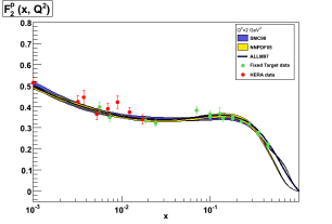
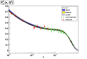
In Tab. 12 we compare our result with the ones in Refs. [13], and [15]. First we notice that the errors are of the same size, while our central values are systematically smaller, with a significant difference for the proton at low Q2superscript𝑄2Q^{2}. A substantial part of effect can be attributed to the different parametrization used for the unpolarized structure function. Indeed, if we evaluate the sum rule of E143 with the SMC98 F2psuperscriptsubscript𝐹2𝑝F_{2}^{p} parametrization [32, 33, 11], at Q2=2GeV2superscript𝑄22superscriptGeV2Q^{2}=2\leavevmode\nobreak\ \mathrm{GeV}^{2} we obtain 0.116±0.008plus-or-minus0.1160.0080.116\pm 0.008 which is less than one sigma away from the result in Refs. [13]; the same happens for the HERMES06 case, using the ALLM parametrization [34] at Q2=2.5GeV2superscript𝑄22.5superscriptGeV2Q^{2}=2.5\leavevmode\nobreak\ \mathrm{GeV}^{2} we get 0.1188±0.0073plus-or-minus0.11880.00730.1188\pm 0.0073. This can be understood looking at Fig. 5 where we compare the different parametrizations for F2psuperscriptsubscript𝐹2𝑝F_{2}^{p} used in the different analysis.

Refer to caption
Refer to caption
Figure 5: Comparison of NNPDF, SMC98 and ALLM parametrizations of the unpolarized structure function F2psuperscriptsubscript𝐹2𝑝F_{2}^{p} in the region where we evaluate the Bjorken sum rule.

It is clear that, while the different F2psuperscriptsubscript𝐹2𝑝F_{2}^{p} parametrizations agree in the kinematical region covered by experimental data, they differ significantly at low-Q2superscript𝑄2Q^{2} in the large-x𝑥x region where there are no data and an extrapolation is needed. For the ALLM and the SMC98 parametrizations the large-x𝑥x behaviour is determined by the chosen functional form; the NNPDF parametrization interpolates by continuity from the last experimental point to the kinematical constrain F2(x=1,Q2)=0subscript𝐹2𝑥1superscript𝑄20F_{2}(x=1,Q^{2})=0. The difference among the parametrizations is then enhanced once we multiply by the asymmetry A1subscript𝐴1A_{1} to reconstruct the polarized structure function g1subscript𝑔1g_{1}.

Target E143 This Analysis
Q2=2GeV2superscript𝑄22GesuperscriptV2Q^{2}=2\mathrm{GeV}^{2}
p 0.120±0.007plus-or-minus0.1200.0070.120\pm 0.007 0.102±0.007plus-or-minus0.1020.0070.102\pm 0.007
d 0.047±0.006plus-or-minus0.0470.0060.047\pm 0.006 0.042±0.005plus-or-minus0.0420.0050.042\pm 0.005
n 0.022±0.013plus-or-minus0.0220.013-0.022\pm 0.013 0.011±0.011plus-or-minus0.0110.011-0.011\pm 0.011
NS 0.149±0.016plus-or-minus0.1490.0160.149\pm 0.016 0.113±0.016plus-or-minus0.1130.0160.113\pm 0.016
Q2=5GeV2superscript𝑄25GesuperscriptV2Q^{2}=5\mathrm{GeV}^{2}
p 0.116±0.007plus-or-minus0.1160.0070.116\pm 0.007 0.106±0.006plus-or-minus0.1060.0060.106\pm 0.006
d 0.043±0.004plus-or-minus0.0430.0040.043\pm 0.004 0.040±0.003plus-or-minus0.0400.0030.040\pm 0.003
n 0.025±0.009plus-or-minus0.0250.009-0.025\pm 0.009 0.018±0.009plus-or-minus0.0180.009-0.018\pm 0.009
NS 0.141±0.013plus-or-minus0.1410.0130.141\pm 0.013 0.124±0.014plus-or-minus0.1240.0140.124\pm 0.014
Target HERMES This Analysis
Q2=2.5GeV2superscript𝑄22.5superscriptGeV2Q^{2}=2.5\mathrm{GeV}^{2}
p 0.1201±0.0090plus-or-minus0.12010.00900.1201\pm 0.0090 0.1055±0.0066plus-or-minus0.10550.00660.1055\pm 0.0066
d 0.0428±0.0035plus-or-minus0.04280.00350.0428\pm 0.0035 0.0416±0.0043plus-or-minus0.04160.00430.0416\pm 0.0043
n 0.0276±0.0093plus-or-minus0.02760.0093-0.0276\pm 0.0093 0.0154±0.0107plus-or-minus0.01540.0107-0.0154\pm 0.0107
NS 0.1477±0.0167plus-or-minus0.14770.01670.1477\pm 0.0167 0.1209±0.0152plus-or-minus0.12090.01520.1209\pm 0.0152
Q2=5GeV2superscript𝑄25GesuperscriptV2Q^{2}=5\mathrm{GeV}^{2}
p 0.1211±0.0092plus-or-minus0.12110.00920.1211\pm 0.0092 0.1097±0.0065plus-or-minus0.10970.00650.1097\pm 0.0065
d 0.0436±0.0035plus-or-minus0.04360.00350.0436\pm 0.0035 0.0407±0.0033plus-or-minus0.04070.00330.0407\pm 0.0033
n 0.0268±0.0094plus-or-minus0.02680.0094-0.0268\pm 0.0094 0.0218±0.0093plus-or-minus0.02180.0093-0.0218\pm 0.0093
NS 0.1479±0.0169plus-or-minus0.14790.01690.1479\pm 0.0169 0.1315±0.0144plus-or-minus0.13150.01440.1315\pm 0.0144
Table 12: Comparison of the integral of g1subscript𝑔1g_{1} over different x𝑥x ranges, at different scales, as determined form the present analysis with the results obtained form by E143, left pad: 0.030.8𝑑xg1(x,Q2)superscriptsubscript0.030.8differential-d𝑥subscript𝑔1𝑥superscript𝑄2\int_{0.03}^{0.8}dxg_{1}(x,Q^{2}) and HERMES, right pad: 0.0210.9𝑑xg1(x,Q2)superscriptsubscript0.0210.9differential-d𝑥subscript𝑔1𝑥superscript𝑄2\int_{0.021}^{0.9}dxg_{1}(x,Q^{2})

Since no neutron target data have been used in our fit, the neutron structure function, g1n,superscriptsubscript𝑔1𝑛g_{1}^{n}, is evaluated from the proton and deuteron ones as

g1n(x,Q2)=2g1d(x,Q2)11.5ωDg1p(x,Q2),superscriptsubscript𝑔1𝑛𝑥superscript𝑄22superscriptsubscript𝑔1𝑑𝑥superscript𝑄211.5subscript𝜔𝐷superscriptsubscript𝑔1𝑝𝑥superscript𝑄2\displaystyle g_{1}^{n}(x,Q^{2})=2\frac{g_{1}^{d}(x,Q^{2})}{1-1.5\omega_{D}}-g_{1}^{p}(x,Q^{2})\,, (32)

where ωDsubscript𝜔𝐷\omega_{D} is the probability of the deuteron to be in the D state; we use ωD=0.05subscript𝜔𝐷0.05\omega_{D}=0.05 which covers most of the published values [35]. We observe that, even if the neutron sum rule is a pure prediction, it is compatible with other estimations.

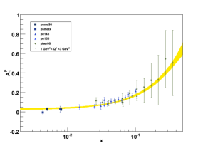
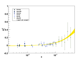
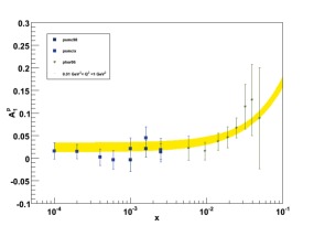
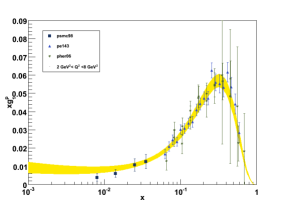
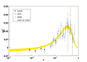
In Fig. 6 we show a comparison of the polarized structure function as extracted in this analysis to data, in the region where we evaluate the Bjorken sum rule. The comparison shows a good agreement.
Refer to caption
Refer to caption
Figure 6: Plot of the structure functions in the region where we evaluate the Bjorken sum rule. The fit curves are taken at Q2=5GeV2superscript𝑄25superscriptGeV2Q^{2}=5\leavevmode\nobreak\ \mathrm{GeV}^{2}.

5.3 Extraction of couplings

In order to extract the strong coupling αssubscript𝛼𝑠\alpha_{s} and the axial coupling gAsubscript𝑔𝐴g_{A} from the values of the Bjorken sum rule we need to extrapolate our fit in the Bjorken variable x𝑥x down to x=0𝑥0x=0 and up to x=1𝑥1x=1.

In this section we discuss the impact of these extrapolations on the extraction of the couplings, and we assess the impact of target mass corrections. Finally we present the results we obtain for αssubscript𝛼𝑠\alpha_{s} and gAsubscript𝑔𝐴g_{A} from our fit. All checks are performed with 100 replicas, while for final results we use the full set of 1000 replicas.

The extrapolation at large–x𝑥x is embedded in the parametrization of F2subscript𝐹2F_{2}, as discussed in the previous section. Therefore we do not need any further assumption to constrain the large–x𝑥x behaviour.

The low–x𝑥x behavior of the structure function g1subscript𝑔1g_{1} is instead very weakly constrained by data, and the Regge behaviour is usually assumed; following Ref. [36] we write:

g1(x,Q2)Axb,similar-to-or-equalssubscript𝑔1𝑥superscript𝑄2𝐴superscript𝑥𝑏g_{1}(x,Q^{2})\simeq A\,x^{b}\,, (33)

with 0<b<0.50𝑏0.50<b<0.5. Such an assumption requires to choose a value of xmatchsubscript𝑥matchx_{\mathrm{match}} such that for x<xmatch𝑥subscript𝑥matchx<x_{\mathrm{match}} the Regge behaviour is assumed to set in. The normalization factor A𝐴A in Eq. 33 is then determined by the matching condition

g1(fit)(xmatch,Q2)=Axmatchb.superscriptsubscript𝑔1fitsubscript𝑥matchsuperscript𝑄2𝐴superscriptsubscript𝑥match𝑏g_{1}^{(\mathrm{fit})}(x_{\mathrm{match}},Q^{2})=A\,x_{\mathrm{match}}^{b}\,. (34)
Q2(GeV2)superscript𝑄2superscriptGeV2Q^{2}(\mathrm{\mathrm{GeV}}^{2}) xmatchsubscript𝑥matchx_{\mathrm{match}} Γ1NS(Q2)superscriptsubscriptΓ1NSsuperscript𝑄2\Gamma_{1}^{\mathrm{NS}}(Q^{2}) Error
1 0.0100 0.12499 0.020989
2 0.0100 0.1356 0.018239
3 0.0100 0.14324 0.017827
4 0.0200 0.13847 0.018275
5 0.0200 0.14322 0.019021
6 0.0200 0.14757 0.020115
7 0.0200 0.15142 0.021429
8 0.0300 0.1458 0.02262
9 0.0300 0.14827 0.023859
10 0.0300 0.15054 0.025165
11 0.0300 0.15265 0.02653
12 0.0500 0.14111 0.027703
13 0.0500 0.14241 0.028749
14 0.0500 0.14366 0.029828
15 0.0500 0.14487 0.030941
16 0.0500 0.14604 0.032087
17 0.0500 0.14718 0.033267
18 0.0500 0.14829 0.03448
19 0.0800 0.13397 0.03552
20 0.0800 0.13461 0.036394
Table 13: First moment of g1subscript𝑔1g_{1} with different values of Q2superscript𝑄2Q^{2}: the error on Γ1NS(Q2)superscriptsubscriptΓ1NSsuperscript𝑄2\Gamma_{1}^{\mathrm{NS}}(Q^{2}) has been added a 100% uncertainty on the low-x𝑥x extrapolation.

In order to choose the matching point, we fix the Regge exponent to 0.20.20.2 and then we proceed as in Ref. [37]: we evaluate the integrals at different values of Q2superscript𝑄2Q^{2} in the range 0<x<10𝑥10<x<1 for different choices of xmatchsubscript𝑥matchx_{\mathrm{match}}, and we look for the minimum value of the error for each value of Q2superscript𝑄2Q^{2}.

From the results collected in Tab. 13 we see that xmatchsubscript𝑥matchx_{\mathrm{match}} grows as Q2superscript𝑄2Q^{2} gets larger. This is understood looking at Fig. 1 where we see that for larger scales the coverage of the data moves towards higher values of x𝑥x.

Once the matching point is been determined, in order to take into account the uncertainty on the value of the Regge exponent and the one on the choice of the matching point, we randomize the Regge exponent in the range 0.1<b<0.50.1𝑏0.5-0.1<b<0.5 and we choose the matching point to be in the range xmatch<x<2xmatchsubscript𝑥match𝑥2subscript𝑥matchx_{\mathrm{match}}<x<2x_{\mathrm{match}}.

In Tab. 14 we present the comparison for the first moment of the structure function g1subscript𝑔1g_{1} evaluated with and without the target mass correction as given in Eq. (17). We observe that the shift on the values of the moment due to the inclusion of these effects is smaller than the experimental error even at the lowest Q2superscript𝑄2Q^{2}.

In principle we could extract gAsubscript𝑔𝐴g_{A}, αssubscript𝛼𝑠\alpha_{s} and the higher-twist term by fitting Eq. (16) evaluated from data at a given value of Q2superscript𝑄2Q^{2}. In practice we evaluate NQ2subscript𝑁superscript𝑄2N_{Q^{2}} different moments taken at different Q2superscript𝑄2Q^{2} in the kinematical region where we have a good coverage by experimental data: 2GeV2Q220GeV22superscriptGeV2superscript𝑄220superscriptGeV22\leavevmode\nobreak\ \mathrm{GeV}^{2}\leq Q^{2}\leq 20\leavevmode\nobreak\ \mathrm{GeV}^{2}. Indeed for Q2>20GeV2superscript𝑄220superscriptGeV2Q^{2}>20\leavevmode\nobreak\ \mathrm{GeV}^{2} the errors on the computed moments become so large that their weighted contribution in the combination is negligible. On the lower side of the energy range we choose to start from Q2=2GeV2superscript𝑄22superscriptGeV2Q^{2}=2\leavevmode\nobreak\ \mathrm{GeV}^{2}, since below this scale a perturbative QCD approach might not be reliable. For this reason we do not fit the higher-twist term, but we will access its contribution by varying the lower cut in Q2superscript𝑄2Q^{2}.

Proton Q2=1GeV2superscript𝑄21superscriptGeV2Q^{2}=1\leavevmode\nobreak\ \mathrm{GeV}^{2} Q2=2GeV2superscript𝑄22superscriptGeV2Q^{2}=2\leavevmode\nobreak\ \mathrm{GeV}^{2}
noTMC 0.1410±0.0109plus-or-minus0.14100.01090.1410\pm 0.0109 0.1264±0.0083plus-or-minus0.12640.00830.1264\pm 0.0083
wTMC 0.1459±0.0116plus-or-minus0.14590.01160.1459\pm 0.0116 0.1276±0.0086plus-or-minus0.12760.00860.1276\pm 0.0086
Deuteron Q2=1GeV2superscript𝑄21superscriptGeV2Q^{2}=1\leavevmode\nobreak\ \mathrm{GeV}^{2} Q2=2GeV2superscript𝑄22superscriptGeV2Q^{2}=2\leavevmode\nobreak\ \mathrm{GeV}^{2}
noTMC 0.0493±0.0141plus-or-minus0.04930.01410.0493\pm 0.0141 0.0350±0.0058plus-or-minus0.03500.00580.0350\pm 0.0058
wTMC 0.0515±0.0158plus-or-minus0.05150.01580.0515\pm 0.0158 0.0355±0.0059plus-or-minus0.03550.00590.0355\pm 0.0059
Table 14: First moment with and without TMC with b=0.2𝑏0.2b=0.2 for the low-x𝑥x extrapolation matched at x=0.001𝑥0.001x=0.001.

We then proceed following the procedure described in detail in Sect. 4.3 of Ref. [38]: the extraction of couplings is done by combining moments at different values of Q2superscript𝑄2Q^{2} in the chosen range and fitting Eq. (16) using MINUIT [39] where gAsubscript𝑔𝐴g_{A} and αssubscript𝛼𝑠\alpha_{s} are the chosen as free parameters. The moments at different Q2superscript𝑄2Q^{2} are correlated, since they are computed using the same fitted parametrization. As detailed in Ref. [38] these correlations induce numerical instabilities in the inversion of the correlation matrix and off-diagonal instabilities due to non-diagonal elements in the correlation matrix becoming dominant. Both these instabilities lead to unreliable results for the extracted couplings.

Q2superscript𝑄2Q^{2} gAsubscript𝑔𝐴g_{A} αs(MZ2)subscript𝛼𝑠superscriptsubscript𝑀𝑍2\alpha_{s}(M_{Z}^{2})
2+5 1.04 ±plus-or-minus\pm 0.12 0.126 ±plus-or-minus\pm 0.005
2+6 1.07 ±plus-or-minus\pm 0.16 0.127 ±plus-or-minus\pm 0.007
2+7 1.08 ±plus-or-minus\pm 0.20 0.128 ±plus-or-minus\pm 0.008
2+8 1.02 ±plus-or-minus\pm 0.21 0.125 ±plus-or-minus\pm 0.012
3+6 1.09 ±plus-or-minus\pm 0.13 0.131 ±plus-or-minus\pm 0.005
3+7 1.12 ±plus-or-minus\pm 0.17 0.132 ±plus-or-minus\pm 0.007
3+8 1.04 ±plus-or-minus\pm 0.20 0.127 ±plus-or-minus\pm 0.013
4+8 1.03 ±plus-or-minus\pm 0.17 0.127 ±plus-or-minus\pm 0.015
Table 15: Fits with different choices of Q2superscript𝑄2Q^{2}.

In order to fix the maximum value of NQ2subscript𝑁superscript𝑄2N_{Q^{2}} for which the extraction of the parameters is numerically stable and reliable, we study the error on the determination of gAsubscript𝑔𝐴g_{A} and αssubscript𝛼𝑠\alpha_{s} as we vary the number of included moments. Once we exclude moments with large correlations, we are left with a small number of combinations, which are showed in Tab. 15.

The combination giving the smallest error (Q2=2,5GeV2superscript𝑄225superscriptGeV2Q^{2}=2,5\leavevmode\nobreak\ \mathrm{GeV}^{2}), once we evaluate asymmetric errors, yields

αs(MZ2)=0.1260.009+0.004,subscript𝛼𝑠superscriptsubscript𝑀𝑍2superscriptsubscript0.1260.0090.004\displaystyle\alpha_{s}(M_{Z}^{2})=0.126_{-0.009}^{+0.004}\,, (35)

for the strong coupling, while the error on gAsubscript𝑔𝐴g_{A} is found to be symmetric.

gAsubscript𝑔𝐴g_{A} αs(MZ2)subscript𝛼𝑠superscriptsubscript𝑀𝑍2\alpha_{s}(M_{Z}^{2}) kFsubscript𝑘𝐹k_{F}
1.02 ±plus-or-minus\pm 0.12 0.126 ±plus-or-minus\pm 0.006 0.5
1.04 ±plus-or-minus\pm 0.12 0.126 ±plus-or-minus\pm 0.005 0.75
1.01 ±plus-or-minus\pm 0.11 0.121 ±plus-or-minus\pm 0.006 1.5
1.03 ±plus-or-minus\pm 0.12 0.120 ±plus-or-minus\pm 0.005 2.0
Table 16: Reference fit (Q2=2,5GeV2superscript𝑄225superscriptGeV2Q^{2}=2,5\leavevmode\nobreak\ \mathrm{GeV}^{2}, NNLO, 1000 reps, kF=1subscript𝑘𝐹1k_{F}=1) compared with variations of the factorization scale.

The only sources of theoretical uncertainty left to consider are the one due to the choice of factorization scale Q=kFmq𝑄subscript𝑘𝐹subscript𝑚𝑞Q=k_{F}m_{q}, which we study by varying kFsubscript𝑘𝐹k_{F} in the range 0.5<kF<20.5subscript𝑘𝐹20.5<k_{F}<2 and to the higher–twist contribution. The results of the variation of the factorization scale are shown in Tab. 16. To take into account the higher–twist contribution we take as an estimate the variation of the central values once the lower Q2superscript𝑄2Q^{2} value is moved up to Q2=3GeV2superscript𝑄23𝐺𝑒superscript𝑉2Q^{2}=3\leavevmode\nobreak\ GeV^{2} (see Tab.15) and down to Q2=1GeV2superscript𝑄21𝐺𝑒superscript𝑉2Q^{2}=1\leavevmode\nobreak\ GeV^{2} (gA=0.99±0.14subscript𝑔𝐴plus-or-minus0.990.14g_{A}=0.99\pm 0.14 and αs(MZ2)=0.117±0.007subscript𝛼𝑠superscriptsubscript𝑀𝑍2plus-or-minus0.1170.007\alpha_{s}(M_{Z}^{2})=0.117\pm 0.007).

In conclusion, we obtain the following result for the determination of the axial coupling gAsubscript𝑔𝐴g_{A} and the strong coupling constant αssubscript𝛼𝑠\alpha_{s}

gAsubscript𝑔𝐴\displaystyle g_{A} =\displaystyle= 1.04±0.12(exp.)0.06+0.05(theo.)=1.04±0.13(tot.)\displaystyle 1.04\pm 0.12({\rm exp.})_{-0.06}^{+0.05}({\rm theo.})=1.04\pm 0.13({\rm tot.}) (36)
αs(MZ2)subscript𝛼𝑠superscriptsubscript𝑀𝑍2\displaystyle\alpha_{s}(M_{Z}^{2}) =\displaystyle= 0.1260.009+0.004(exp.)0.011+0.005(theo.)=0.1260.014+0.006(tot.),\displaystyle 0.126_{-0.009}^{+0.004}({\rm exp.})_{-0.011}^{+0.005}({\rm theo.})=0.126_{-0.014}^{+0.006}({\rm tot.})\,,

which are compatible with previous extractions [42, 43] from polarized DIS and the Bjorken sum rule.

6 Conclusions

We extracted a parametrization of the spin asymmetries A1p,dsuperscriptsubscript𝐴1𝑝𝑑A_{1}^{p,d}, based on all available DIS data using the Monte-Carlo sampling techniques and neural networks as basic interpolation tools. We checked in the process that the statistical methods developed for the unpolarized studies by the NNPDF Collaboration can be naturally extended to handle the new data sets considered in this work. Our main result is an effective tool, which we used to test different assumptions needed to reconstruct the polarized structure function g1subscript𝑔1g_{1}. As an example of possible applications we compared to previous estimations of experimental sum rules, and we found that the used parametrization for the unpolarized structure function F2subscript𝐹2F_{2} can be a sizable source of error at low values of Q2superscript𝑄2Q^{2}. We also performed a study of the Bjorken sum rule, and the extraction of the axial coupling and the strong coupling, obtaining values which are compatible with previous analysis.

It would be interesting to compare the results obtained for the Bjorken sum rule when determined from global QCD fits to polarized DIS, SDIS and hadron-hadron collisions data, like the one presented in [44], especially once W𝑊W production data from RHIC will be included in such fits, providing an extra constraints on the light flavours separation.

The present study is also meant to be a first step towards the application of the NNPDF techniques to the determination of a set of polarized PDFs with a faithful error estimation.

Acknowledgments.
We thank S. Forte, G. Ridolfi and M. Anselmino for useful discussion and suggestions. We are greatly indebted to R. De Vita (CLAS), L. De Nardo and A. Fantoni (HERMES), A. Bressan (COMPASS) and T. S. Toole (E155) for detailed information on experimental data. The work of LDD is supported by an STFC Advanced Fellowship.

Appendix A Experimental errors

Experimentally, we have

A||CfPbPtNN+N+N+,\displaystyle A_{||}\simeq\frac{C}{fP_{b}P_{t}}\frac{N_{-}-N_{+}}{N_{-}+N_{+}}\,, (37)

where

  • C𝐶C is a nuclear correction that depends on the material the target is made of;

  • f𝑓f is the dilution factor which accounts for the fact that only a fraction of the target nucleons is polarizable;

  • Pbsubscript𝑃𝑏P_{b} and Ptsubscript𝑃𝑡P_{t} are the beam and target polarizations;

  • N(+)subscript𝑁N_{-(+)} is the number of scattered electrons/muons per incident charge for negative (positive) beam helicity.

Thus, most of the errors quoted by experiments are normalization errors.

  • EMC [10]: A2=0subscript𝐴20A_{2}=0 is assumed; 9.6% overall normalization due to beam and target polarization; multiplicative errors on R𝑅R and f𝑓f; additive errors on A2subscript𝐴2A_{2}, the false asymmetry K𝐾K and the radiative correction.

  • SMC98 [11]: A2=0subscript𝐴20A_{2}=0 is assumed; multiplicative errors on Ptsubscript𝑃𝑡P_{t}, Pbsubscript𝑃𝑏P_{b}, R𝑅R, f𝑓f and the polarized background ΔPbgΔsubscript𝑃𝑏𝑔\Delta P_{bg}; additive errors on A2subscript𝐴2A_{2}, the false asymmetry ΔAfalseΔsubscript𝐴𝑓𝑎𝑙𝑠𝑒\Delta A_{false}, the radiative correction and the momentum resolution.

  • SMC low-x𝑥x [12]: A2=0subscript𝐴20A_{2}=0 is assumed; multiplicative errors on Ptsubscript𝑃𝑡P_{t}, Pbsubscript𝑃𝑏P_{b}, R𝑅R, f𝑓f and the polarized background ΔPbgΔsubscript𝑃𝑏𝑔\Delta P_{bg}; additive errors on A2subscript𝐴2A_{2}, the false asymmetry ΔAfalseΔsubscript𝐴𝑓𝑎𝑙𝑠𝑒\Delta A_{false} and the radiative correction.

  • E143 [13]: g2subscript𝑔2g_{2} is evaluated using the Wandzura-Wilczeck relation

    g2WW(x,Q2)=g1(x,Q2)+x1dyyg1(x,Q2),superscriptsubscript𝑔2𝑊𝑊𝑥superscript𝑄2subscript𝑔1𝑥superscript𝑄2superscriptsubscript𝑥1𝑑𝑦𝑦subscript𝑔1𝑥superscript𝑄2\displaystyle g_{2}^{WW}(x,Q^{2})=-g_{1}(x,Q^{2})+\int_{x}^{1}\frac{dy}{y}g_{1}(x,Q^{2})\,, (38)

    using and empirical fit of g1/F1=axα(1+bx+cx2)(1+Cf(Q2))subscript𝑔1subscript𝐹1𝑎superscript𝑥𝛼1𝑏𝑥𝑐superscript𝑥21𝐶𝑓superscript𝑄2g_{1}/F_{1}=ax^{\alpha}(1+bx+cx^{2})(1+Cf(Q^{2})); multiplicative errors on Ptsubscript𝑃𝑡P_{t}, Pbsubscript𝑃𝑏P_{b}, f𝑓f and the nuclear correction C𝐶C which account for a total 3.7% for the proton and 4.9% for the deuteron; additive uncorrelated error on the radiative corrections.

  • E155 [14]: g2subscript𝑔2g_{2} is evaluated in the same way of E143, but the parameters of the fitted functional form have different values; we will add as a shift the difference between A1subscript𝐴1A_{1} and g1/F1subscript𝑔1subscript𝐹1g_{1}/F_{1}; multiplicative errors on Ptsubscript𝑃𝑡P_{t}, Pbsubscript𝑃𝑏P_{b}, f𝑓f and the nuclear correction C𝐶C which account for a total 7.6% for the proton; additive uncorrelated error on the radiative corrections.

  • HERMES06 [15]: a parametrization for g2subscript𝑔2g_{2} is fitted to existing data; normalizations errors of 5.2% for the proton and 5% included in the systematic quoted for each data point; additional additive error on the parametrization used for g2subscript𝑔2g_{2}.

  • COMPASS [16]: A2=0subscript𝐴20A_{2}=0 is assumed; multiplicative errors on Ptsubscript𝑃𝑡P_{t}, Pbsubscript𝑃𝑏P_{b}, the dilution factor f𝑓f and the depolarization factor D𝐷D; additive errors on the false asymmetry and the radiative correction.

References

  • [1] S. Forte, L. Garrido, J. I. Latorre and A. Piccione, JHEP 0205 (2002) 062 [arXiv:hep-ph/0204232].
  • [2] L. Del Debbio, S. Forte, J. I. Latorre, A. Piccione and J. Rojo [NNPDF Collaboration], JHEP 0503, 080 (2005) [arXiv:hep-ph/0501067].
  • [3] L. Del Debbio, S. Forte, J. I. Latorre, A. Piccione and J. Rojo [NNPDF Collaboration], JHEP 0703 (2007) 039 [arXiv:hep-ph/0701127].
  • [4] R. D. Ball et al. [NNPDF Collaboration], Nucl. Phys.  B 809 (2009) 1 [arXiv:0808.1231 [hep-ph]].
  • [5] R. D. Ball et al. [The NNPDF Collaboration], arXiv:0906.1958 [hep-ph].
  • [6] J. Blumlein and H. Bottcher, Nucl. Phys.  B 636, 225 (2002) [arXiv:hep-ph/0203155].
  • [7] J. Blumlein and A. Guffanti, AIP Conf. Proc.  792, 261 (2005).
  • [8] M. Anselmino, A. Efremov and E. Leader, Phys. Rept.  261, 1 (1995) [Erratum-ibid.  281, 399 (1997)] [arXiv:hep-ph/9501369].
  • [9] S. E. Kuhn, J. P. Chen and E. Leader, arXiv:0812.3535 [hep-ph].
  • [10] J. Ashman et al. [European Muon Collaboration], Nucl. Phys. B 328 (1989) 1.
  • [11] B. Adeva et al. [Spin Muon Collaboration], Phys. Rev.  D 58 (1998) 112001.
  • [12] B. Adeva et al. [Spin Muon Collaboration], Phys. Rev. D 60, 072004 (1999) [Erratum-ibid. D 62, 079902 (2000)].
  • [13] K. Abe et al. [E143 collaboration], Phys. Rev. D 58, 112003 (1998) [arXiv:hep-ph/9802357].
  • [14] P. L. Anthony et al. [E155 Collaboration], Phys. Lett. B 493 (2000) 19 [arXiv:hep-ph/0007248].
  • [15] A. Airapetian et al. [HERMES Collaboration], Phys. Rev.  D 75 (2007) 012007 [arXiv:hep-ex/0609039].
  • [16] E. S. Ageev et al. [COMPASS Collaboration], Phys. Lett. B 612 (2005) 154 [arXiv:hep-ex/0501073].
  • [17] M. Dittmar et al., arXiv:0901.2504 [hep-ph].
  • [18] G. D’Agostini, Bayesian reasoning in data analysis: A critical introduction, World Scientific, 2003.
  • [19] C. M. Bishop, Neural Networks for Pattern Recognition, Oxford University Press, Oxford 1995.
  • [20] K. Hornik, M. Stinchcombe and H. White, Neural Networks, vol. 2, 359 (1989).
  • [21] M. Mitchell, An introduction to genetic algorithms, MIT Press, 1998
  • [22] J. I. Latorre and J. Rojo, JHEP 0401, 055 (2004).
  • [23] S. Matsuda and T. Uematsu, Nucl. Phys.  B 168 (1980) 181.
  • [24] A. Piccione and G. Ridolfi, Nucl. Phys.  B 513 (1998) 301 [arXiv:hep-ph/9707478].
  • [25] J. Blumlein and A. Tkabladze, Nucl. Phys.  B 553 (1999) 427 [arXiv:hep-ph/9812478].
  • [26] A. Accardi and W. Melnitchouk, Phys. Lett.  B 670 (2008) 114 [arXiv:0808.2397 [hep-ph]].
  • [27] C. Simolo, arXiv:0807.1501 [hep-ph].
  • [28] S. A. Larin and J. A. M. Vermaseren, Phys. Lett.  B 259 (1991) 345.
  • [29] S. Wandzura and F. Wilczek, Phys. Lett.  B 72 (1977) 195.
  • [30] L. W. Whitlow, S. Rock, A. Bodek, E. M. Riordan and S. Dasu, Phys. Lett. B 250 (1990) 193.
  • [31] K. Abe et al. [E143 Collaboration], Phys. Lett. B 452, 194 (1999) [arXiv:hep-ex/9808028].
  • [32] A. Milsztajn, A. Staude, K. M. Teichert, M. Virchaux and R. Voss, Z. Phys.  C 49 (1991) 527.
  • [33] M. Arneodo et al. [New Muon Collaboration.], Phys. Lett.  B 364 (1995) 107 [arXiv:hep-ph/9509406].
  • [34] H. Abramowicz and A. Levy, arXiv:hep-ph/9712415.
  • [35] W. Buck and F. Gross, Phys. Rev. D 20, 2361 (1979), M. Z. Zuilhof and J. A. Tjon, Phys. Rev. C 22, 2369 (1980), M. Lacombe et al., ibid. 21, 861 (1980), R. Machleidt et al., Phys. Rep. 149, 1 (1987)
  • [36] F. E. Close and R. G. Roberts, Phys. Lett.  B 336 (1994) 257 [arXiv:hep-ph/9407204].
  • [37] R. Abbate and S. Forte, Phys. Rev.  D 72 (2005) 117503 [arXiv:hep-ph/0511231].
  • [38] S. Forte, J. I. Latorre, L. Magnea and A. Piccione, Nucl. Phys.  B 643 (2002) 477 [arXiv:hep-ph/0205286].
  • [39] F. James and M. Roos, Comput. Phys. Commun.  10, 343 (1975).
  • [40] A. Deur et al., Phys. Rev. Lett.  93 (2004) 212001 [arXiv:hep-ex/0407007].
  • [41] A. Deur et al., Phys. Rev.  D 78 (2008) 032001 [arXiv:0802.3198 [nucl-ex]].
  • [42] G. Altarelli, R. D. Ball, S. Forte and G. Ridolfi, Nucl. Phys.  B 496 (1997) 337 [arXiv:hep-ph/9701289].
  • [43] G. Altarelli, R. D. Ball, S. Forte and G. Ridolfi, Acta Phys. Polon.  B 29 (1998) 1145 [arXiv:hep-ph/9803237].
  • [44] D. de Florian, R. Sassot, M. Stratmann and W. Vogelsang, arXiv:0904.3821 [hep-ph].