]Also at Center for Nonlinear Phenomena and Complex Systems,
Université Libre de Bruxelles, Code Postal 231, Campus Plaine, B-1050 Brussels, Belgium.
Extracting chemical energy by growing disorder: Efficiency at maximum power
Abstract
We consider the efficiency of chemical energy extraction from the environment by the growth of a copolymer made of two constituent units in the entropy-driven regime. We show that the thermodynamic nonlinearity associated with the information processing aspect is responsible for a branching of the system properties such as power, speed of growth, entropy production, and efficiency, with varying affinity. The standard linear thermodynamics argument which predicts an efficiency of at maximum power is inappropriate because the regime of maximum power is located either outside of the linear regime or on a separate bifurcated branch, and because the usual thermodynamic force is not the natural variable for this optimization.
pacs:
05.70.Ln,05.70.-a,05.40.-aI Introduction
Carnot efficiency is one of the cornerstones of thermodynamics since it leads to the definition of entropy and the Second Law of thermodynamics. It expresses a fundamental limitation on how much work can be extracted from a heat flow. A less studied but arguably more relevant question for many isothermal chemical and biological processes is how much chemical energy a system can extract from its environment by increasing the system’s configurational entropy. Thermodynamics does, in fact, also prescribe a limit, even though at first sight it appears to be almost trivial: the energy extracted by such an isothermal transfer can be carried out with efficiency. However, there is a crucial additional condition, namely, that this efficiency can only be reached – just as in the case of Carnot efficiency – by a reversible, infinitely slow process. Hence efficiency is achieved for a process with zero power output. The question of efficiencies at finite power should thus be addressed.
In the context of thermal machines, a straightforward analysis based on linear irreversible thermodynamics teaches us that, as one moves away from the reversible regime, the power goes through a unique maximum, and that the efficiency at this maximum is, at most, VandenBroeck05 ; EspLindBroeckPRL . The same argument can easily be extended to the transformation between different forms of chemical energy. However, the above prediction may not apply for several reasons. First, the point of maximum power does not necessarily lie in the linear regime. Second, thermodynamic nonlinear effects can give rise to bifurcated branches. Finally, the above-mentioned efficiency is attained upon maximization with respect to the thermodynamic force associated with the power generating flux. While this is a natural set-up in many problems, it may not always correspond to the relevant scenario.
In this paper, we investigate the efficiency of a chemical entropy-driven process of capital importance in biophysics, namely, copolymer synthesis Bennett79 ; 08AndrieuxGaspardPNAS ; 09AndrieuxGaspardJCP ; JarzynskiPNAS , see also Volkenstein ; Smith . As exemplified by the copolymer DNA, guardian of genetic information, such processes are essential for biological information processing. We will show that the above-mentioned complications are present in this generic model. In particular, the thermodynamic nonlinearity associated with the information processing aspect is responsible for a branching of the systems properties such as power, speed of growth, efficiency and entropy production, as one varies the affinity. Furthermore, the regime of maximum power is located either outside of the linear regime or on the separate bifurcated branch. Finally, it turns out that the thermodynamic force is not a natural control variable in the present model. While our (exact) analysis is carried out for the simplest possible model, namely, copolymer synthesis with two constituent building blocks, our findings suggest that chemical information processing usually operates in the far-from-equilibrium regime, with unique features due to the entropic contribution.
In Sec. II we present the basic thermodynamic formulas that define our system. In Sec. III we present the detailed kinetic description of our model, whose results are discussed in detail in Sec. IV. In particular, it is here that we exhibit the correct and unexpected results for the efficiency at maximum power, results that arise entirely from the nonlinear nature of the problem. A brief recapitulation is presented in Sec. V.
II Thermodynamics
We begin with some well-known relations for isothermal systems. Consider a spontaneous chemical process involving particles of different types labeled by , with corresponding particle number and chemical potential . The system is in thermal and mechanical equilibrium at temperature and pressure . The total Gibbs free energy
| (1) |
evolves toward a minimum value, so that . Alternatively, to characterize the evolution of the isothermal system we write
| (2) | |||||
We have separated the total entropy change into two contributions. The first one, , is the always-positive part of the entropy change, called the internal entropy production. The other is the contribution to the entropy change due to exchange processes between the system and its environment, and can be positive or negative. Associated with these contributions, we have written the change in he number of particles of type as
| (3) |
where the first contribution is due to exchange of particles with the environment, and the second is the internal change caused by the chemical reaction. We take the system to be closed, i.e., it exchanges only energy but not particles with the environment, so that . These definitions lead to consistency between the statements that the system evolves toward a minimum in the Gibbs free energy and that the internal entropy production of this chemical system has to be positive Prigogine , that is,
| (4) |
Obviously, for a reversible transformation with zero internal entropy production .
We now turn to the simplest scenario of copolymer synthesis. The system consists of a bulk-phase containing two types of monomer units, and , which can attach or detach at the endpoint of a single linear copolymer. We identify the four states , , and . Here represent free bulk monomers and represent monomers attached to the copolymer. Since the number of each type of monomer is conserved, one has and . The entropy production (4) can thus be written in the familiar bilinear form
| (5) | |||||
with the affinities and the conjugate fluxes .
In view of the relation , we rewrite the entropy production as
| (6) |
Here is the change of enthalpy per monomer upon transfer from the bulk to the copolymer. The crucial point, which has been discussed in detail in the literature Bennett79 ; 08AndrieuxGaspardPNAS ; 09AndrieuxGaspardJCP ; JarzynskiPNAS , is to realize that the average change of entropy upon transfer of a monomer from the bulk to the copolymer contains two contributions. One is the monomer entropy, , due to the change in the monomer degrees of freedom and in the monomer internal structure between the free monomer in solution and the monomer inside the copolymer. The other is the configurational entropy denoted by , due to the change in the information stored in the polymer sequence that occurrs when a monomer is added to the copolymer. It is given by the Shannon entropy
| (7) |
where is the copolymer length in monomer units and is the probability of a copolymer with monomer sequence . In the absence of correlations, the Shannon entropy is expressed solely in terms of the monomer abundance probabilities and ,
| (8) |
For simplicity, we further assume that monomer entropy and enthalpy changes upon transfer of a monomer from the bulk to the copolymer and vice versa have the same value for both monomers, that is,
| (9) |
We henceforth call the monomer “free enthalpy.” Introducing the net speed of growth of the copolymer, , the entropy production can finally be written as
| (10) |
where the total affinity is given by
| (11) |
The expression (10) for the entropy production in the steady state regime of the growing copolymer has been derived in Refs. Bennett79 ; 08AndrieuxGaspardPNAS ; JarzynskiPNAS ; 09AndrieuxGaspardJCP . It is interesting to realize that the affinity is not an obvious control parameter due to its dependence on which is in turn a nontrivial function of . Only can be easily controlled externally by changing the concentration of the monomers in solution.
The power at which , the free enthalpy divided by temperature, is extracted from the surroundings by copolymer growth is given by
| (12) |
The efficiency of the process is defined as the ratio of this power over the cost of the entropy growth per unit time,
| (13) |
In the reversible limit with , the efficiency of the process becomes optimal, , but the extracted power goes to zero. The standard prediction from linear thermodynamics that arrives at an efficiency of at maximum power is obtained upon expanding the velocity in terms of the affinity, , with the linear response coefficient. Within this approximation the power becomes . Note that this power attains its maximum for with the corresponding efficiency , if we assume that is kept constant. However, below we will investigate the more natural optimization with respect of , since this is the natural and easily controllable variable related to the free enthalpy flux. Whatever control variable is used, we will see in Sec. IV that the true maximum is beyond the reach of this linear expansion (and even of a nonlinear continuation of this expansion).
III Kinetics
We now turn to the detailed kinetic description of the copolymerization process, which will allow us to identify the expressions for and in the context of a full nonlinear analysis. Let us call and the rates of insertion and removal, respectively, of monomer . Because the free enthalpy of the monomers has been assumed to be the same, the ratios of the reaction rates are given by
| (14) |
The fraction of monomers of type present in the copolymer in the regime of steady growth can be determined by the following self-consistency argument. The ratio of the number of versus monomers in an ensemble of copolymers has to be equal to the ratio of their net rates of attachment. For monomer , this net rate is the pure rate of attachment, , minus the rate of detachment, which is . The factor arises from the fact that detachment is only possible when the monomer at the tip of the copolymer is of type , and this occurs with probability . The net rate of attachment for is similarly given by . We thus conclude that
| (15) |
The solution of the resulting quadratic equation for reads
| (16) |
where . By a similar argument we find that the speed of growth of the copolymer, given by the rate of attachment minus the rate of detachment , is given by
| (17) |
We note from Eqs. (8), (10), (11), (16) and (17) that equilibrium, and , occurs at with and . For smaller (larger) values of , () and the copolymer is synthesized (degraded), i.e., (). Of specific interest to us is the surprising regime of entropy-driven growth, and , but with Bennett79 ; 08AndrieuxGaspardPNAS ; 09AndrieuxGaspardJCP ; JarzynskiPNAS . Under the simplifications assumed in our model, this occurs when . Monomers are pumped uphill against the free enthalpy barrier under the influence of the entropic contribution to the affinity. The power (enthalpy per unit time) extracted from the copolymerization dynamics is positive in this entropy driven regime, cf. Eq. (12), with corresponding efficiency given in Eq. (13).
IV Efficiency at maximum power
|
|---|
|
|
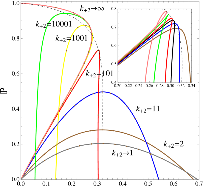
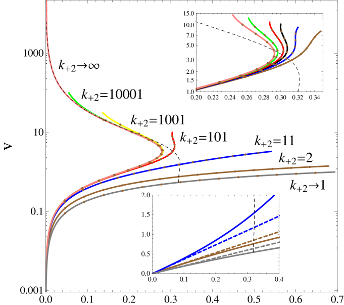
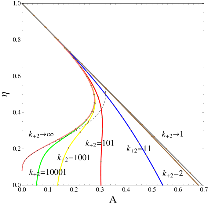
To study the main question of interest, namely, the regime of maximum power and its corresponding efficiency, we choose convenient variables. We note that the model is described by four kinetic constants, but the latter are not independent since they obey the relation Eq. (14). Furthermore, one of them can be set equal to by an appropriate choice of the time unit, e.g., . As the remaining two degrees of freedom, we choose and . We then have explicit functional expressions for all the other quantities , , and , cf. Eqs. (16) and (17), and hence also , , , , and , see Eqs. (11), (12), (13), (8) and (10). Other relations between, for example, and , can then be obtained by parametric elimination. The quantities , , , , and can easily be calculated numerically. The results are summarized in Figs. 1, 2, 3, and 4. We next turn to a discussion of these figures, supplemented with corresponding analytic calculations.
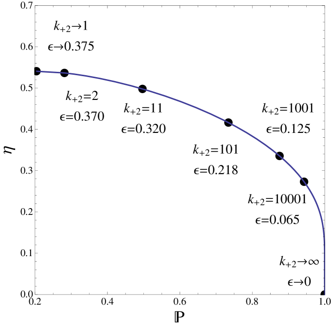
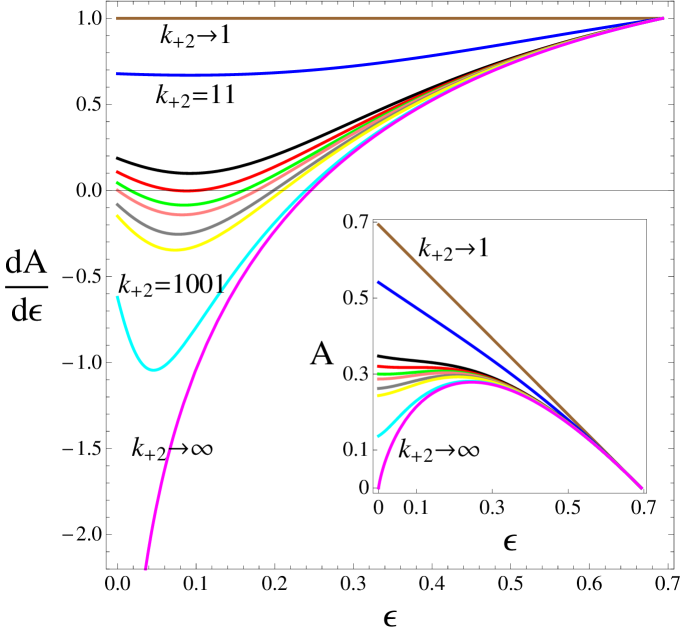
The information contained in Fig.1 is detailed in the caption. The most striking feature in this figure is the existence of two different branches for the power and velocity in terms of the affinity. The transition between the two branches occurs when
| (18) |
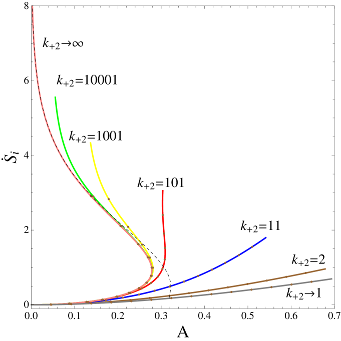
diverges. indicates or . Since is an analytic function of , the new branch appears when touches zero. As long as the latter quantity remains positive, which is the case for smaller than a certain critical value, cf. Fig. 3, the power and velocity can be seen as a true function of . Branching takes place at the critical point, characterized by , resulting in and , see again Fig. 3. For values of larger than this critical value, power is no longer a proper function of , as two branches appear, with two values of for a given value of . While along the linear branch and its continuation the affinity decreases with , the affinity increases with on the new lower branch, cf. the inset in Fig. 3. This remarkable result implies that we can approach low values of affinities via a nonlinear branch which is distinct from the branch predicted by linear response theory and its continuation. We note that the entropy production itself becomes a bi-valued function in terms of the affinity, as can be seen in Fig. 4. Naively, one would expect that entropy production and affinity both provide consistent measures for the distance from equilibrium. This is clearly not the case in the present model, where the entropy production is a decreasing function of the affinity on the upper nonlinear branch. In particular, for very large values of one finds that the entropy production becomes very large while the affinity goes to zero. We conclude that the affinity is not a reliable measure for the distance from equilibrium.
To explore the region close to equilibrium and, in particular, the linear response regime, we write and expand in powers of . From Eq. (8) with Eqs. (16) and (14) we find
| (19) |
where
| (20) |
For the affinity, we find from Eq. (11) that
| (21) |
The efficiency thus becomes
| (22) | |||||
This linear dependence of the efficiency on the affinity close to equilibrium is clearly identified in the upper left region of the third affinity plot in Fig. 1, while the corresponding behavior of the affinity in terms of , cf. Eq. (21), is observed in the lower left region of the inset of Fig. 3. In this regime close to equilibrium we find the standard linear response relations
| (23) | |||||
| (24) |
with the Onsager coefficient given by , cf. the lower left regions of the power and speed plots in Fig. 1. Note also that the Onsager coefficient becomes independent of in the limit , where .
We have seen that linear response predicts an efficiency at maximum power of . However, as announced earlier, this result is not correct. This is seen in Fig. 1 or in Fig. 2, where the affinity is clearly above the value in the regime “closest” to equilibrium. The explanation is that maximum power occurs beyond the reach of linear response theory, as can clearly be seen in the lower inset of the plot in Fig. 1, where the linear response curves (dashed lines) become inaccurate at maximum power. Furthermore, we note that the point of maximum power moves onto the nonlinear branch as grows, now occurring at decreasing values of . So, even though we are approaching a regime of low power output with decreasing affinity, we do so via the nonlinear branch, where the prediction of linear response theory utterly fails. The main conclusion is that, while there is indeed a regime of linear response, it is unable to describe the region of maximum power, which always occurs outside the regime of validity of the linear law.
To complete our analysis, we explore in detail the limiting cases and . For transparency, we explicitly retain instead of setting it equal to unity. In the limit where , we find that
| (25) |
This leads to an efficiency , as observed in Fig. 1. In this limit, the value of leading to maximum power is obtained as the solution of the transcendental equation , namely, . At maximum power we thus get
| (26) |
as seen in Figs. 1 and 2. As an immediate consequence, we also find and , as observed in Fig. 1.
In the limit , where
| (27) |
the efficiency reads . The numerical results of Fig. 1 suggest that maximum power in this limit occurs for very close to zero. We therefore expand the velocity around and find . Using Eq. (12), we find that maximum power occurs at , resulting in . For the latter becomes
| (28) |
as observed in Figs. 1 and 2. Similarly, by expanding to first order around and using the value we found for at maximum power, we find that
| (29) |
V Conclusions
Using a simple model of copolymerization, we have shown that free enthalpy can be extracted from the environment in response to the entropic force corresponding to the information stored in a growing copolymer sequence. The thermodynamic nonlinearity associated with the information processing aspect is responsible for a branching of the dependence on the affinity of system properties such as power, speed of growth and efficiency. The nonlinear regime occuring after the branching is particularly surprising since the entropy production keeps increasing even as the affinity begins to decrease. We identified a regime of linear response where the efficiency of the energy extraction is optimal (equal to ), but where, as usual, the power output goes to zero. Considering instead the efficiency at maximum power, we found that the universal prediction of linear response theory (efficiency equal to ) is inappropriate for this model. The reason is that the copolymerization generating maximum power occurs far from equilibrium in a region not accessible to linear response theory. Our results suggest a possible self-powering mechanism for nonequilibrium systems that can extract chemical energy from their surroundings by growing their internal structural information.
Acknowledgments
M. E. is supported by the FNRS Belgium (chargé de recherches) and by the government of Luxembourg (Bourse de formation recherches). This work was partially supported by the National Science Foundation under grant No. PHY-0354937.
References
- (1) C. Van den Broeck, Phys. Rev. Lett. 95, 190602, (2005); Adv. Chem. Phys. 135, 189 (2007).
- (2) M. Esposito, K. Lindenberg and C. Van den Broeck, PRL 102, 130602 (2009).
- (3) C. H. Bennett, BioSystems 11, 85 (1979).
- (4) D. Andrieux and P. Gaspard, PNAS 105, 9516 (2008).
- (5) C. Jarzynski, PNAS 105, 9451 (2008).
- (6) D. Andrieux and P. Gaspard, J. Chem. Phys. 130, 014901 (2009).
- (7) M.V. Volkenstein, Molecular Biophysics (Academic Press, New York, 1977).
- (8) E. Smith, J. Theo. Biol. 252, 198 (2008).
- (9) D. Kondepudi and I. Prigogine, Modern thermodynamics (Wiley, Chichester, 1998).