1. Introduction
From the regular hexagon of unit size remove circular
holes of small radius ε > 0 𝜀 0 \varepsilon>0 H ε subscript 𝐻 𝜀 H_{\varepsilon} | H ε | = 3 3 2 − 2 π ε 2 subscript 𝐻 𝜀 3 3 2 2 𝜋 superscript 𝜀 2 |H_{\varepsilon}|=\frac{3\sqrt{3}}{2}-2\pi\varepsilon^{2} ( 𝐱 , ω ) ∈ H ε × [ 0 , 2 π ] 𝐱 𝜔 subscript 𝐻 𝜀 0 2 𝜋 ({\mathbf{x}},\omega)\in H_{\varepsilon}\times[0,2\pi] τ ε hex ( 𝐱 , ω ) superscript subscript 𝜏 𝜀 hex 𝐱 𝜔 \tau_{\varepsilon}^{\mathrm{hex}}({\mathbf{x}},\omega) free path length (or first exit time ).
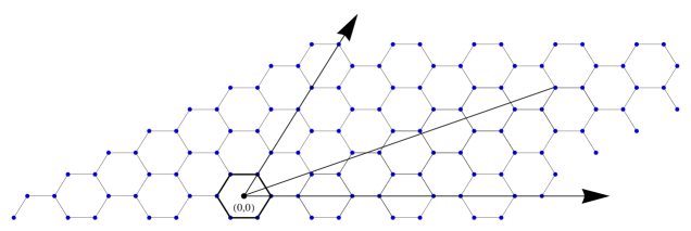
Equivalently, one can consider the unit honeycomb tessellation of the
euclidean plane, with “fat points” (obstacles or
scatterers) of radius ε 𝜀 \varepsilon m e 1 + n j 𝑚 subscript e 1 𝑛 j m\textbf{e}_{1}+n\textbf{j} m ≢ n ( mod 3 ) not-equivalent-to 𝑚 annotated 𝑛 pmod 3 m\nequiv n\pmod{3} Λ 6 = ℤ e 1 + ℤ j = ℤ 2 ( 1 0 1 / 2 3 / 2 ) subscript Λ 6 ℤ subscript e 1 ℤ j superscript ℤ 2 1 0 1 2 3 2 \Lambda_{6}={\mathbb{Z}}\textbf{e}_{1}+{\mathbb{Z}}\textbf{j}={\mathbb{Z}}^{2}\left(\begin{smallmatrix}1&0\\
1/2&\sqrt{3}/2\end{smallmatrix}\right) j = ( 1 2 , 3 2 ) j 1 2 3 2 \textbf{j}=\big{(}\frac{1}{2},\frac{\sqrt{3}}{2}\big{)} ω 𝜔 \omega 1 𝐱 𝐱 {\mathbf{x}} τ ε hex ( 𝐱 , ω ) superscript subscript 𝜏 𝜀 hex 𝐱 𝜔 \tau_{\varepsilon}^{\mathrm{hex}}({\mathbf{x}},\omega)
ℙ ε hex ( ξ ) = 1 2 π | H ε | | { ( 𝐱 , ω ) ∈ H ε × [ 0 , 2 π ] : ε τ ε hex ( 𝐱 , ω ) > ξ } | , ξ ∈ [ 0 , ∞ ) , formulae-sequence superscript subscript ℙ 𝜀 hex 𝜉 1 2 𝜋 subscript 𝐻 𝜀 conditional-set 𝐱 𝜔 subscript 𝐻 𝜀 0 2 𝜋 𝜀 superscript subscript 𝜏 𝜀 hex 𝐱 𝜔 𝜉 𝜉 0 {\mathbb{P}}_{\varepsilon}^{\mathrm{hex}}(\xi)=\frac{1}{2\pi|H_{\varepsilon}|}\left|\big{\{}({\mathbf{x}},\omega)\in H_{\varepsilon}\times[0,2\pi]:\varepsilon\tau_{\varepsilon}^{\mathrm{hex}}({\mathbf{x}},\omega)>\xi\big{\}}\right|,\quad\xi\in[0,\infty), (1.1)
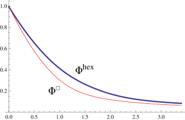
that ε τ ε hex ( 𝐱 , ω ) > ξ 𝜀 superscript subscript 𝜏 𝜀 hex 𝐱 𝜔 𝜉 \varepsilon\tau_{\varepsilon}^{\mathrm{hex}}({\mathbf{x}},\omega)>\xi ε → 0 + → 𝜀 superscript 0 \varepsilon\rightarrow 0^{+} Φ hex ( ξ ) = lim ε → 0 + ℙ ε hex ( ξ ) superscript Φ hex 𝜉 subscript → 𝜀 superscript 0 superscript subscript ℙ 𝜀 hex 𝜉 \Phi^{\mathrm{hex}}(\xi)=\lim_{\varepsilon\rightarrow 0^{+}}{\mathbb{P}}_{\varepsilon}^{\mathrm{hex}}(\xi) ξ ⩾ 0 𝜉 0 \xi\geqslant 0 Φ hex ( ξ ) superscript Φ hex 𝜉 \Phi^{\mathrm{hex}}(\xi)
The version of this problem where the initial point is chosen to
be the center of the hexagon has been solved in [3 ] . The
square lattice analog of estimating (1.1 [14 ] and G.
Pólya [19 ] . A complete solution was given in [7 ] . A
detailed history and presentation of various ideas and tools
involved in this and related problems, as well as a description of
recent developments in the study of the periodic Lorentz gas,
including [10 , 11 , 12 , 16 , 17 , 18 ] , is provided in [13 , 15 ] .
\path (65,6.1499)(377.53,134.29) \path (0,0)(25,-43.3)(75,-43.3)(100,0)(150,0)(175,-43.3)(225,-43.3)(250,0)(300,0)(325,-43.3)(375,-43.3)(400,0)
\path \path \path \path \path \path \path \path \path \path \path \path \path \path ∙ ∙ \bullet ∙ ∙ \bullet C 1 subscript 𝐶 1 C_{1} ∙ ∙ \bullet C 2 subscript 𝐶 2 C_{2} ∙ ∙ \bullet C 2 ′ superscript subscript 𝐶 2 ′ C_{2}^{\prime} ∙ ∙ \bullet C 3 subscript 𝐶 3 C_{3} ∙ ∙ \bullet C 3 ′ superscript subscript 𝐶 3 ′ C_{3}^{\prime} ∙ ∙ \bullet C 4 subscript 𝐶 4 C_{4} ∙ ∙ \bullet C 4 ′ superscript subscript 𝐶 4 ′ C_{4}^{\prime} ∙ ∙ \bullet C 5 subscript 𝐶 5 C_{5} ∙ ∙ \bullet C 5 ′ superscript subscript 𝐶 5 ′ C_{5}^{\prime} ∙ ∙ \bullet C 6 subscript 𝐶 6 C_{6} ∙ ∙ \bullet C 6 ′ superscript subscript 𝐶 6 ′ C_{6}^{\prime} ∙ ∙ \bullet C 7 subscript 𝐶 7 C_{7} ∙ ∙ \bullet C 7 ′ superscript subscript 𝐶 7 ′ C_{7}^{\prime} ∘ \circ ∘ \circ ∘ \circ ∘ \circ ∘ \circ ∘ \circ ∘ \circ ∘ \circ ∘ \circ ∘ \circ ∘ \circ ∘ \circ ∘ \circ ∘ \circ ∘ \circ ∘ \circ ∘ \circ ∘ \circ ∘ \circ ∘ \circ ∘ \circ ∘ \circ ∘ \circ ∘ \circ ∘ \circ ∘ \circ ∘ \circ ∘ \circ ∘ \circ ∘ \circ ∘ \circ ∘ \circ ∘ \circ ∘ \circ ∘ \circ ∘ \circ ω 𝜔 \omega \arc 95-0.390 \arc 98-0.3930 𝐱 𝐱 {\mathbf{x}} \path (90.43,16.576)(21.29,-36.87)(96.52,-5.1)(94.39,9.717)(50.94,43.3)(4.1,7.074)(2.53,-4.39) \path (65,6.14199)(150,6.14199)
\path Figure 1. The free path in a hexagonal billiard and respectively in a
hexagonal lattice
One additional difficulty encountered here is the absence of a
theory of continued fractions in the case of the hexagonal
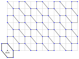
tessellation. To bypass this obstacle we shall deform this tessellation, as in
[3 ] , into ℤ ( 3 ) 2 = { ( m , n ) ∈ ℤ 2 , m ≢ n ( mod 3 ) } subscript superscript ℤ 2 3 formulae-sequence 𝑚 𝑛 superscript ℤ 2 not-equivalent-to 𝑚 annotated 𝑛 pmod 3 {\mathbb{Z}}^{2}_{(3)}=\{(m,n)\in{\mathbb{Z}}^{2},m\nequiv n\pmod{3}\} [9 , 7 ] in the situation of the square lattice, or
equivalently the corresponding tiling of ℝ 2 superscript ℝ 2 {\mathbb{R}}^{2} 6 ( mod 3 ) pmod 3 \pmod{3}
Theorem 1 .
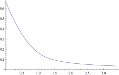
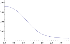
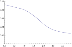
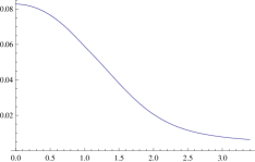
There exists a decreasing continuous function Φ hex : [ 0 , ∞ ) → ( 0 , ∞ ) : superscript Φ hex → 0 0 \Phi^{\mathrm{hex}}:[0,\infty)\rightarrow(0,\infty) Φ hex ( 0 ) = 1 superscript Φ hex 0 1 \Phi^{\mathrm{hex}}(0)=1 Φ hex ( ∞ ) = 0 superscript Φ hex 0 \Phi^{\mathrm{hex}}(\infty)=0 δ > 0 𝛿 0 \delta>0 ε → 0 + → 𝜀 superscript 0 \varepsilon\rightarrow 0^{+}
ℙ ε hex ( ξ ) = Φ hex ( ξ ) + O δ ( ε 1 8 − δ ) , ∀ ξ ⩾ 0 , formulae-sequence superscript subscript ℙ 𝜀 hex 𝜉 superscript Φ hex 𝜉 subscript 𝑂 𝛿 superscript 𝜀 1 8 𝛿 for-all 𝜉 0 {\mathbb{P}}_{\varepsilon}^{\mathrm{hex}}(\xi)=\Phi^{\mathrm{hex}}(\xi)+O_{\delta}\big{(}\varepsilon^{\frac{1}{8}-\delta}\big{)},\quad\forall\xi\geqslant 0,
uniformly for ξ 𝜉 \xi [ 0 , ∞ ) 0 [0,\infty) C 1 , C 2 > 0 subscript 𝐶 1 subscript 𝐶 2
0 C_{1},C_{2}>0
C 1 ξ ⩽ Φ hex ( ξ ) ⩽ C 2 ξ , ∀ ξ ∈ [ 1 , ∞ ) . formulae-sequence subscript 𝐶 1 𝜉 superscript Φ hex 𝜉 subscript 𝐶 2 𝜉 for-all 𝜉 1 \frac{C_{1}}{\xi}\leqslant\Phi^{\mathrm{hex}}(\xi)\leqslant\frac{C_{2}}{\xi},\quad\forall\xi\in[1,\infty). (1.2)
Estimate (1.2 Φ hex superscript Φ hex \Phi^{\mathrm{hex}}
Φ hex ( ξ ) = 4 π 2 G ( 2 ξ 3 ) , superscript Φ hex 𝜉 4 superscript 𝜋 2 𝐺 2 𝜉 3 \Phi^{\mathrm{hex}}(\xi)=\frac{4}{\pi^{2}}\ G\left(\frac{2\xi}{\sqrt{3}}\right), (1.3)
with G ( ξ ) 𝐺 𝜉 G(\xi) ζ ( 2 ) c I G I , Q ( ∗ ) 𝜁 2 subscript 𝑐 𝐼 superscript subscript 𝐺 𝐼 𝑄
\frac{\zeta(2)}{c_{I}}G_{I,Q}^{(*)} 5.22 6.6 6.7 6.8 6.9 6.10 6.11 7.1 7.2 7.5 7.6 7.8 7.11 7.12 7.13 8.1 8.2 8.5 8.6 8.8 8.9 8.10 8.11 8.12 8.13 8.14 9.1 9.2 9.4 9.5 9.6 9.7 9.9 9.10 9.11 9.12 9.13 9.14 9.15 9.16
In the case of the square lattice only the term from (5.22 2 3 2 3 \frac{2}{\sqrt{3}} ξ 𝜉 \xi Φ □ superscript Φ □ \Phi^{\square} 1.2
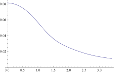
Figure 2. The limiting repartition functions Φ hex superscript Φ hex \Phi^{\mathrm{hex}} Φ □ superscript Φ □ \Phi^{\square}
In the case of a lattice it was actually proved in [16 ] that for
every 𝐱 ∈ ℝ 2 ∖ ℚ 2 𝐱 superscript ℝ 2 superscript ℚ 2 {\mathbf{x}}\in{\mathbb{R}}^{2}\setminus{\mathbb{Q}}^{2} lim ε → 0 + 1 2 π | { ω ∈ [ 0 , 2 π ) : ε τ ε □ ( 𝐱 , ω ) > ξ } | = Φ □ ( ξ ) subscript → 𝜀 superscript 0 1 2 𝜋 conditional-set 𝜔 0 2 𝜋 𝜀 superscript subscript 𝜏 𝜀 □ 𝐱 𝜔 𝜉 superscript Φ □ 𝜉 \lim_{\varepsilon\rightarrow 0^{+}}\frac{1}{2\pi}\big{|}\big{\{}\omega\in[0,2\pi):\varepsilon\tau_{\varepsilon}^{\square}({\mathbf{x}},\omega)>\xi\big{\}}\big{|}=\Phi^{\square}(\xi) 𝐱 𝐱 {\mathbf{x}}
The analog problem about the free path length in a regular polygon with
n 𝑛 n n ≠ 3 , 4 , 6 𝑛 3 4 6
n\neq 3,4,6 [20 ] may prove helpful.
2. Translating the problem to the square lattice with mod 3 modulo absent 3 \mod{3}
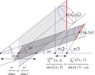
For manifest symmetry reasons it suffices to consider 𝐱 ∈ H ε 𝐱 subscript 𝐻 𝜀 {\mathbf{x}}\in H_{\varepsilon} ω ∈ [ 0 , π 6 ] 𝜔 0 𝜋 6 \omega\in\big{[}0,\frac{\pi}{6}\big{]} t = tan ω ∈ [ 0 , 1 3 ] 𝑡 𝜔 0 1 3 t=\tan\omega\in\big{[}0,\frac{1}{\sqrt{3}}\big{]} τ ε hex ( 𝐱 , ω ) = τ ε hex ( 𝐱 , t ) superscript subscript 𝜏 𝜀 hex 𝐱 𝜔 subscript superscript 𝜏 hex 𝜀 𝐱 𝑡 \tau_{\varepsilon}^{\mathrm{hex}}({\mathbf{x}},\omega)=\tau^{\mathrm{hex}}_{\varepsilon}({\mathbf{x}},t) [3 ]
consider the lattice ℤ 2 M 0 superscript ℤ 2 subscript 𝑀 0 {\mathbb{Z}}^{2}M_{0} M 0 = ( 1 0 1 / 2 3 / 2 ) subscript 𝑀 0 1 0 1 2 3 2 M_{0}=\left(\begin{smallmatrix}1&0\\
1/2&\sqrt{3}/2\end{smallmatrix}\right) T 𝐱 = 𝐱 M 0 − 1 𝑇 𝐱 𝐱 superscript subscript 𝑀 0 1 T{\mathbf{x}}={\mathbf{x}}M_{0}^{-1} ℝ 2 superscript ℝ 2 {\mathbb{R}}^{2}
T ( x , y ) = ( x − y 3 , 2 y 3 ) = ( x ′ , y ′ ) . 𝑇 𝑥 𝑦 𝑥 𝑦 3 2 𝑦 3 superscript 𝑥 ′ superscript 𝑦 ′ T(x,y)=\left(x-\frac{y}{\sqrt{3}},\frac{2y}{\sqrt{3}}\right)=(x^{\prime},y^{\prime}).
This maps the vertices ( q + a 2 , a 3 2 ) 𝑞 𝑎 2 𝑎 3 2 \big{(}q+\frac{a}{2},\frac{a\sqrt{3}}{2}\big{)} ( q , a ) 𝑞 𝑎 (q,a) ℤ 2 superscript ℤ 2 {\mathbb{Z}}^{2} ℤ ( 3 ) 2 subscript superscript ℤ 2 3 {\mathbb{Z}}^{2}_{(3)} ℤ 2 superscript ℤ 2 {\mathbb{Z}}^{2} q ≢ a ( mod 3 ) not-equivalent-to 𝑞 annotated 𝑎 pmod 3 q\nequiv a\pmod{3} 3 x 𝑥 x T 𝑇 T S q , a , ε = ( x 0 , y 0 ) + ε ( cos θ , sin θ ) subscript 𝑆 𝑞 𝑎 𝜀
subscript 𝑥 0 subscript 𝑦 0 𝜀 𝜃 𝜃 S_{q,a,\varepsilon}=(x_{0},y_{0})+\varepsilon(\cos\theta,\sin\theta) ( x 0 , y 0 ) = ( q + a 2 , a 3 2 ) subscript 𝑥 0 subscript 𝑦 0 𝑞 𝑎 2 𝑎 3 2 (x_{0},y_{0})=\big{(}q+\frac{a}{2},\frac{a\sqrt{3}}{2}\big{)} ( x 0 ′ , y 0 ′ ) + ε ( cos θ − sin θ 3 , 2 sin θ 3 ) superscript subscript 𝑥 0 ′ superscript subscript 𝑦 0 ′ 𝜀 𝜃 𝜃 3 2 𝜃 3 (x_{0}^{\prime},y_{0}^{\prime})+\varepsilon\big{(}\cos\theta-\frac{\sin\theta}{\sqrt{3}},\frac{2\sin\theta}{\sqrt{3}}\big{)} ( x 0 ′ , y 0 ′ ) = ( q , a ) = T ( x 0 , y 0 ) superscript subscript 𝑥 0 ′ superscript subscript 𝑦 0 ′ 𝑞 𝑎 𝑇 subscript 𝑥 0 subscript 𝑦 0 (x_{0}^{\prime},y_{0}^{\prime})=(q,a)=T(x_{0},y_{0}) w = 2 ε 𝑤 2 𝜀 w=2\varepsilon t = tan ω 𝑡 𝜔 t=\tan\omega S q , a , ε subscript 𝑆 𝑞 𝑎 𝜀
S_{q,a,\varepsilon} 4 w ′ = 2 ε ′ cos ω ′ superscript 𝑤 ′ 2 superscript 𝜀 ′ superscript 𝜔 ′ w^{\prime}=2\varepsilon^{\prime}\cos\omega^{\prime} T ( S q , a , ε ) 𝑇 subscript 𝑆 𝑞 𝑎 𝜀
T(S_{q,a,\varepsilon}) t ′ = tan ω ′ = Ψ ( t ) superscript 𝑡 ′ superscript 𝜔 ′ Ψ 𝑡 t^{\prime}=\tan\omega^{\prime}=\Psi(t)
Ψ : [ 0 , 1 3 ] → [ 0 , 1 ] , t ′ = Ψ ( t ) = 2 t 3 − t , t = Ψ − 1 ( t ′ ) = t ′ 3 t ′ + 2 . \Psi:\left[0,\frac{1}{\sqrt{3}}\right]\rightarrow[0,1],\quad t^{\prime}=\Psi(t)=\frac{2t}{\sqrt{3}-t},\quad t=\Psi^{-1}(t^{\prime})=\frac{t^{\prime}\sqrt{3}}{t^{\prime}+2}.
The intersection of these two channels and the x 𝑥 x
2 ε sin ω = w sin ω = w ′ sin ω ′ = 2 ε ′ tan ω ′ . 2 𝜀 𝜔 𝑤 𝜔 superscript 𝑤 ′ superscript 𝜔 ′ 2 superscript 𝜀 ′ superscript 𝜔 ′ \frac{2\varepsilon}{\sin\omega}=\frac{w}{\sin\omega}=\frac{w^{\prime}}{\sin\omega^{\prime}}=\frac{2\varepsilon^{\prime}}{\tan\omega^{\prime}}.
In particular
ε ′ = ε ′ ( ω , ε ) = ε tan ω ′ sin ω = ε cos ( π / 6 + ω ) . superscript 𝜀 ′ superscript 𝜀 ′ 𝜔 𝜀 𝜀 superscript 𝜔 ′ 𝜔 𝜀 𝜋 6 𝜔 \varepsilon^{\prime}=\varepsilon^{\prime}(\omega,\varepsilon)=\frac{\varepsilon\tan\omega^{\prime}}{\sin\omega}=\frac{\varepsilon}{\cos(\pi/6+\omega)}. (2.1)
Figure 3. The free path length in the honeycomb and in
the deformed honeycomb
Figure 4. Change of scatterers under the linear transformation T 𝑇 T
We can first replace each circular scatterer S q , a , ε subscript 𝑆 𝑞 𝑎 𝜀
S_{q,a,\varepsilon} S ~ q , a , ε subscript ~ 𝑆 𝑞 𝑎 𝜀
\tilde{S}_{q,a,\varepsilon} ( x 0 , y 0 ) subscript 𝑥 0 subscript 𝑦 0 (x_{0},y_{0}) π 3 𝜋 3 \frac{\pi}{3} 2 ε cos ( π / 6 + ω ) = 2 ε ′ 2 𝜀 𝜋 6 𝜔 2 superscript 𝜀 ′ \frac{2\varepsilon}{\cos(\pi/6+\omega)}=2\varepsilon^{\prime} 3 4 ω 𝜔 \omega τ ε hex ( 𝐱 , t ) superscript subscript 𝜏 𝜀 hex 𝐱 𝑡 \tau_{\varepsilon}^{\mathrm{hex}}({\mathbf{x}},t) τ ~ ε hex ( 𝐱 , t ) superscript subscript ~ 𝜏 𝜀 hex 𝐱 𝑡 \tilde{\tau}_{\varepsilon}^{\mathrm{hex}}({\mathbf{x}},t) 4 3 ε 2 4 3 superscript 𝜀 2 4\sqrt{3}\varepsilon^{2}
Next we apply T 𝑇 T ( mod 3 ) pmod 3 \pmod{3} T − 1 superscript 𝑇 1 T^{-1} H 𝐻 H T ( H ) 𝑇 𝐻 T(H) ( 0 , 0 ) 0 0 (0,0) 4 T ( H ) 𝑇 𝐻 T(H) F 𝐹 F [ 0 , 1 ) 2 superscript 0 1 2 [0,1)^{2} [ − 1 , 0 ) × [ 0 , 1 ) 1 0 0 1 [-1,0)\times[0,1) [ 0 , 1 ) × [ − 1 , 0 ) 0 1 1 0 [0,1)\times[-1,0) ε ′ = ε ′ ( ω , ε ) superscript 𝜀 ′ superscript 𝜀 ′ 𝜔 𝜀 \varepsilon^{\prime}=\varepsilon^{\prime}(\omega,\varepsilon) 2.1 t ′ = tan ω ′ superscript 𝑡 ′ superscript 𝜔 ′ t^{\prime}=\tan\omega^{\prime} V ε ′ = { 0 } × [ − ε ′ , ε ′ ] subscript 𝑉 superscript 𝜀 ′ 0 superscript 𝜀 ′ superscript 𝜀 ′ V_{\varepsilon^{\prime}}=\{0\}\times[-\varepsilon^{\prime},\varepsilon^{\prime}]
q ~ ε ′ □ ( 𝐱 ′ , t ′ ) = inf { n ∈ ℕ 0 : 𝐱 ′ + ( n , n t ′ ) ∈ ℤ ( 3 ) 2 + V ε ′ } , superscript subscript ~ 𝑞 superscript 𝜀 ′ □ superscript 𝐱 ′ superscript 𝑡 ′ infimum conditional-set 𝑛 subscript ℕ 0 superscript 𝐱 ′ 𝑛 𝑛 superscript 𝑡 ′ subscript superscript ℤ 2 3 subscript 𝑉 superscript 𝜀 ′ \tilde{q}_{\varepsilon^{\prime}}^{\square}({\mathbf{x}}^{\prime},t^{\prime})=\inf\{n\in{\mathbb{N}}_{0}:{\mathbf{x}}^{\prime}+(n,nt^{\prime})\in{\mathbb{Z}}^{2}_{(3)}+V_{\varepsilon^{\prime}}\},
the horizontal free path length in the square lattice with vertical
scatterers of (nonconstant) length 2 ε ′ 2 superscript 𝜀 ′ 2\varepsilon^{\prime} ( x 0 ′ , y 0 ′ ) = ( q , a ) ∈ ℤ ( 3 ) 2 superscript subscript 𝑥 0 ′ superscript subscript 𝑦 0 ′ 𝑞 𝑎 subscript superscript ℤ 2 3 (x_{0}^{\prime},y_{0}^{\prime})=(q,a)\in{\mathbb{Z}}^{2}_{(3)} q ε 0 □ ( 𝐱 ′ , t ′ ) superscript subscript 𝑞 subscript 𝜀 0 □ superscript 𝐱 ′ superscript 𝑡 ′ q_{\varepsilon_{0}}^{\square}({\mathbf{x}}^{\prime},t^{\prime}) constant length 2 ε 0 2 subscript 𝜀 0 2\varepsilon_{0} ( x 0 ′ , y 0 ′ ) = ( q , a ) ∈ ℤ ( 3 ) 2 superscript subscript 𝑥 0 ′ superscript subscript 𝑦 0 ′ 𝑞 𝑎 subscript superscript ℤ 2 3 (x_{0}^{\prime},y_{0}^{\prime})=(q,a)\in{\mathbb{Z}}^{2}_{(3)} q ε + □ ( 𝐱 ′ , t ′ ) ⩽ q ~ ε ′ □ ( 𝐱 ′ , t ′ ) ⩽ q ε − □ ( 𝐱 ′ , t ′ ) subscript superscript 𝑞 □ subscript 𝜀 superscript 𝐱 ′ superscript 𝑡 ′ subscript superscript ~ 𝑞 □ superscript 𝜀 ′ superscript 𝐱 ′ superscript 𝑡 ′ subscript superscript 𝑞 □ subscript 𝜀 superscript 𝐱 ′ superscript 𝑡 ′ q^{\square}_{\varepsilon_{+}}({\mathbf{x}}^{\prime},t^{\prime})\leqslant\tilde{q}^{\square}_{\varepsilon^{\prime}}({\mathbf{x}}^{\prime},t^{\prime})\leqslant q^{\square}_{\varepsilon_{-}}({\mathbf{x}}^{\prime},t^{\prime}) t ′ superscript 𝑡 ′ t^{\prime} I ′ superscript 𝐼 ′ I^{\prime} ε − ⩽ ε ′ = ε ′ ( t ′ ) ⩽ ε + subscript 𝜀 superscript 𝜀 ′ superscript 𝜀 ′ superscript 𝑡 ′ superscript 𝜀 \varepsilon_{-}\leqslant\varepsilon^{\prime}=\varepsilon^{\prime}(t^{\prime})\leqslant\varepsilon^{+} ∀ t ′ ∈ I ′ for-all superscript 𝑡 ′ superscript 𝐼 ′ \forall t^{\prime}\in I^{\prime}
For each angle ω ′ superscript 𝜔 ′ \omega^{\prime} T 𝑇 T H 𝐻 H F 𝐹 F T − 1 superscript 𝑇 1 T^{-1} [1 , 7 , 9 ] (see also the expository paper [13 ] ). Removal of vertical scatterers
V q , a , ε ′ = T ( S ~ q , a , ε ) subscript 𝑉 𝑞 𝑎 superscript 𝜀 ′
𝑇 subscript ~ 𝑆 𝑞 𝑎 𝜀
V_{q,a,\varepsilon^{\prime}}=T(\tilde{S}_{q,a,\varepsilon}) q ≡ a ( mod 3 ) 𝑞 annotated 𝑎 pmod 3 q\equiv a\pmod{3} ℤ ( 3 ) 2 subscript superscript ℤ 2 3 {\mathbb{Z}}^{2}_{(3)} T − 1 superscript 𝑇 1 T^{-1}
τ ~ ε hex ( 𝐱 , t ) sin ( 2 π / 3 ) = q ~ ε ′ □ ( T 𝐱 , t ′ ) sin ( π / 3 − ω ) = q ~ ε ′ □ ( T 𝐱 , t ′ ) cos ( π / 6 + ω ) . subscript superscript ~ 𝜏 hex 𝜀 𝐱 𝑡 2 𝜋 3 subscript superscript ~ 𝑞 □ superscript 𝜀 ′ 𝑇 𝐱 superscript 𝑡 ′ 𝜋 3 𝜔 subscript superscript ~ 𝑞 □ superscript 𝜀 ′ 𝑇 𝐱 superscript 𝑡 ′ 𝜋 6 𝜔 \frac{\tilde{\tau}^{\mathrm{hex}}_{\varepsilon}({\mathbf{x}},t)}{\sin(2\pi/3)}=\frac{\tilde{q}^{\square}_{\varepsilon^{\prime}}(T{\mathbf{x}},t^{\prime})}{\sin(\pi/3-\omega)}=\frac{\tilde{q}^{\square}_{\varepsilon^{\prime}}(T{\mathbf{x}},t^{\prime})}{\cos(\pi/6+\omega)}.
This shows that
τ ~ ε hex ( 𝐱 , t ) > ξ ε ⟺ q ~ ε ′ □ ( T 𝐱 , t ′ ) > 2 ξ cos ( π / 6 + ω ) ε 3 = ξ ′ ε ′ , ξ ′ := 2 ξ 3 , formulae-sequence formulae-sequence subscript superscript ~ 𝜏 hex 𝜀 𝐱 𝑡 𝜉 𝜀 ⟺
subscript superscript ~ 𝑞 □ superscript 𝜀 ′ 𝑇 𝐱 superscript 𝑡 ′ 2 𝜉 𝜋 6 𝜔 𝜀 3 superscript 𝜉 ′ superscript 𝜀 ′ assign superscript 𝜉 ′ 2 𝜉 3 \tilde{\tau}^{\mathrm{hex}}_{\varepsilon}({\mathbf{x}},t)>\frac{\xi}{\varepsilon}\quad\Longleftrightarrow\quad\tilde{q}^{\square}_{\varepsilon^{\prime}}(T{\mathbf{x}},t^{\prime})>\frac{2\xi\cos(\pi/6+\omega)}{\varepsilon\sqrt{3}}=\frac{\xi^{\prime}}{\varepsilon^{\prime}},\quad\xi^{\prime}:=\frac{2\xi}{\sqrt{3}}, (2.2)
leading to
χ ( ξ ε , ∞ ) ( τ ~ ε hex ( 𝐱 , t ) ) = χ ( ξ ′ ε ′ , ∞ ) ( q ~ ε ′ □ ( T 𝐱 , t ′ ) ) , ∀ 𝐱 ∈ H , ∀ t ∈ [ 0 , 1 3 ] . formulae-sequence subscript 𝜒 𝜉 𝜀 superscript subscript ~ 𝜏 𝜀 hex 𝐱 𝑡 subscript 𝜒 superscript 𝜉 ′ superscript 𝜀 ′ subscript superscript ~ 𝑞 □ superscript 𝜀 ′ 𝑇 𝐱 superscript 𝑡 ′ formulae-sequence for-all 𝐱 𝐻 for-all 𝑡 0 1 3 \chi_{\big{(}\frac{\xi}{\varepsilon},\infty\big{)}}\Big{(}\tilde{\tau}_{\varepsilon}^{\mathrm{hex}}({\mathbf{x}},t)\Big{)}=\chi_{\big{(}\frac{\xi^{\prime}}{\varepsilon^{\prime}},\infty\big{)}}\Big{(}\tilde{q}^{\square}_{\varepsilon^{\prime}}(T{\mathbf{x}},t^{\prime})\Big{)},\quad\forall{\mathbf{x}}\in H,\forall t\in\left[0,\frac{1}{\sqrt{3}}\right].
For each interval I = [ tan ω 0 , tan ω 1 ] ⊆ [ 0 , 1 3 ] 𝐼 subscript 𝜔 0 subscript 𝜔 1 0 1 3 I=[\tan\omega_{0},\tan\omega_{1}]\subseteq\big{[}0,\frac{1}{\sqrt{3}}\big{]}
ε I − := ε cos ( π / 6 + ω 0 ) ⩽ ε ′ = ε cos ( π / 6 + ω ) ⩽ ε I + := ε cos ( π / 6 + ω 1 ) , ε I ± = ( 1 + O | I | ) ) ε . \begin{split}\varepsilon^{-}_{I}:=\frac{\varepsilon}{\cos(\pi/6+\omega_{0})}\leqslant\varepsilon^{\prime}&=\frac{\varepsilon}{\cos(\pi/6+\omega)}\leqslant\varepsilon^{+}_{I}:=\frac{\varepsilon}{\cos(\pi/6+\omega_{1})},\\
\varepsilon^{\pm}_{I}&=\big{(}1+O|I|)\big{)}\varepsilon.\end{split}
Employing now (2.2 ε ↦ q ~ ε □ ( T 𝐱 , t ′ ) maps-to 𝜀 superscript subscript ~ 𝑞 𝜀 □ 𝑇 𝐱 superscript 𝑡 ′ \varepsilon\mapsto\tilde{q}_{\varepsilon}^{\square}(T{\mathbf{x}},t^{\prime})
ξ I − := ξ ′ ε I − ε I + ⩽ ξ ′ ⩽ ξ I + := ξ ′ ε I + ε I − , ξ I ± = ( 1 + O ( | I | ) ) ξ ′ , formulae-sequence assign subscript superscript 𝜉 𝐼 superscript 𝜉 ′ subscript superscript 𝜀 𝐼 subscript superscript 𝜀 𝐼 superscript 𝜉 ′ subscript superscript 𝜉 𝐼 assign superscript 𝜉 ′ subscript superscript 𝜀 𝐼 subscript superscript 𝜀 𝐼 subscript superscript 𝜉 plus-or-minus 𝐼 1 𝑂 𝐼 superscript 𝜉 ′ \xi^{-}_{I}:=\frac{\xi^{\prime}\varepsilon^{-}_{I}}{\varepsilon^{+}_{I}}\leqslant\xi^{\prime}\leqslant\xi^{+}_{I}:=\frac{\xi^{\prime}\varepsilon^{+}_{I}}{\varepsilon^{-}_{I}},\quad\xi^{\pm}_{I}=\big{(}1+O(|I|)\big{)}\xi^{\prime},
we infer
χ ( ξ I + ε I + , ∞ ) ( q ε I + □ ( T 𝐱 , t ′ ) ) = χ ( ξ ′ ε I − , ∞ ) ( q ε I + □ ( T 𝐱 , t ′ ) ) ⩽ χ ( ξ ′ ε ′ , ∞ ) ( q ε I + □ ( T 𝐱 , t ′ ) ) ⩽ χ ( ξ ′ ε ′ , ∞ ) ( q ~ ε ′ □ ( T 𝐱 , t ′ ) ) = χ ( ξ ε , ∞ ) ( τ ~ ε hex ( 𝐱 , t ) ) ⩽ χ ( ξ ′ ε ′ , ∞ ) ( q ε I − □ ( T 𝐱 , t ′ ) ) ⩽ χ ( ξ ′ ε I + , ∞ ) ( q ε I − □ ( T 𝐱 , t ′ ) ) = χ ( ξ I − ε I − , ∞ ) ( q ε I − □ ( T 𝐱 , t ′ ) ) . subscript 𝜒 subscript superscript 𝜉 𝐼 subscript superscript 𝜀 𝐼 superscript subscript 𝑞 subscript superscript 𝜀 𝐼 □ 𝑇 𝐱 superscript 𝑡 ′ subscript 𝜒 superscript 𝜉 ′ subscript superscript 𝜀 𝐼 superscript subscript 𝑞 subscript superscript 𝜀 𝐼 □ 𝑇 𝐱 superscript 𝑡 ′ subscript 𝜒 superscript 𝜉 ′ superscript 𝜀 ′ superscript subscript 𝑞 subscript superscript 𝜀 𝐼 □ 𝑇 𝐱 superscript 𝑡 ′ subscript 𝜒 superscript 𝜉 ′ superscript 𝜀 ′ subscript superscript ~ 𝑞 □ superscript 𝜀 ′ 𝑇 𝐱 superscript 𝑡 ′ subscript 𝜒 𝜉 𝜀 subscript superscript ~ 𝜏 hex 𝜀 𝐱 𝑡 subscript 𝜒 superscript 𝜉 ′ superscript 𝜀 ′ superscript subscript 𝑞 subscript superscript 𝜀 𝐼 □ 𝑇 𝐱 superscript 𝑡 ′ subscript 𝜒 superscript 𝜉 ′ subscript superscript 𝜀 𝐼 superscript subscript 𝑞 subscript superscript 𝜀 𝐼 □ 𝑇 𝐱 superscript 𝑡 ′ subscript 𝜒 subscript superscript 𝜉 𝐼 subscript superscript 𝜀 𝐼 superscript subscript 𝑞 subscript superscript 𝜀 𝐼 □ 𝑇 𝐱 superscript 𝑡 ′ \begin{split}\chi_{\big{(}\frac{\xi^{+}_{I}}{\varepsilon^{+}_{I}},\infty\big{)}}\Big{(}q_{\varepsilon^{+}_{I}}^{\square}(T{\mathbf{x}},t^{\prime})\Big{)}&=\chi_{\big{(}\frac{\xi^{\prime}}{\varepsilon^{-}_{I}},\infty\big{)}}\Big{(}q_{\varepsilon^{+}_{I}}^{\square}(T{\mathbf{x}},t^{\prime})\Big{)}\leqslant\chi_{\big{(}\frac{\xi^{\prime}}{\varepsilon^{\prime}},\infty\big{)}}\Big{(}q_{\varepsilon^{+}_{I}}^{\square}(T{\mathbf{x}},t^{\prime})\Big{)}\\
&\leqslant\chi_{\big{(}\frac{\xi^{\prime}}{\varepsilon^{\prime}},\infty\big{)}}\Big{(}\tilde{q}^{\square}_{\varepsilon^{\prime}}(T{\mathbf{x}},t^{\prime})\Big{)}=\chi_{\big{(}\frac{\xi}{\varepsilon},\infty\big{)}}\Big{(}\tilde{\tau}^{\mathrm{hex}}_{\varepsilon}({\mathbf{x}},t)\Big{)}\leqslant\chi_{\big{(}\frac{\xi^{\prime}}{\varepsilon^{\prime}},\infty\big{)}}\Big{(}q_{\varepsilon^{-}_{I}}^{\square}(T{\mathbf{x}},t^{\prime})\Big{)}\\
&\leqslant\chi_{\big{(}\frac{\xi^{\prime}}{\varepsilon^{+}_{I}},\infty\big{)}}\Big{(}q_{\varepsilon^{-}_{I}}^{\square}(T{\mathbf{x}},t^{\prime})\Big{)}=\chi_{\big{(}\frac{\xi^{-}_{I}}{\varepsilon^{-}_{I}},\infty\big{)}}\Big{(}q_{\varepsilon^{-}_{I}}^{\square}(T{\mathbf{x}},t^{\prime})\Big{)}.\end{split}
Consider
𝔾 I , ε ( ξ ) := ∫ Ψ ( I ) d t ′ t ′ 2 + t ′ + 1 ∫ F 𝑑 𝐱 ′ χ ( ξ ε , ∞ ) ( q ε □ ( 𝐱 ′ , t ′ ) ) . assign subscript 𝔾 𝐼 𝜀
𝜉 subscript Ψ 𝐼 𝑑 superscript 𝑡 ′ superscript 𝑡 ′ 2
superscript 𝑡 ′ 1 subscript 𝐹 differential-d superscript 𝐱 ′ subscript 𝜒 𝜉 𝜀 subscript superscript 𝑞 □ 𝜀 superscript 𝐱 ′ superscript 𝑡 ′ \mathbb{G}_{I,\varepsilon}(\xi):=\int_{\Psi(I)}\frac{dt^{\prime}}{t^{\prime 2}+t^{\prime}+1}\int_{F}d{\mathbf{x}}^{\prime}\,\chi_{\big{(}\frac{\xi}{\varepsilon},\infty\big{)}}\Big{(}q^{\square}_{\varepsilon}({\mathbf{x}}^{\prime},t^{\prime})\Big{)}. (2.3)
Applying the change of variable ( 𝐱 ′ , t ′ ) = ( T 𝐱 , Ψ ( t ) ) superscript 𝐱 ′ superscript 𝑡 ′ 𝑇 𝐱 Ψ 𝑡 ({\mathbf{x}}^{\prime},t^{\prime})=\big{(}T{\mathbf{x}},\Psi(t)\big{)} 2.3 d 𝐱 = 3 2 d 𝐱 ′ 𝑑 𝐱 3 2 𝑑 superscript 𝐱 ′ d{\mathbf{x}}=\frac{\sqrt{3}}{2}d{\mathbf{x}}^{\prime} d t t 2 + 1 = 3 2 ⋅ d t ′ t ′ 2 + t ′ + 1 𝑑 𝑡 superscript 𝑡 2 1 ⋅ 3 2 𝑑 superscript 𝑡 ′ superscript 𝑡 ′ 2
superscript 𝑡 ′ 1 \frac{dt}{t^{2}+1}=\frac{\sqrt{3}}{2}\cdot\frac{dt^{\prime}}{t^{\prime 2}+t^{\prime}+1}
3 4 𝔾 I , ε I + ( ξ I + ) ⩽ 3 4 ∫ Ψ ( I ) d t ′ t ′ 2 + t ′ + 1 ∫ F 𝑑 𝐱 ′ χ ( ξ I + ε I + , ∞ ) ( q ε I + □ ( 𝐱 ′ , t ′ ) ) ⩽ ℙ ~ I , ε ( ξ ) := ∬ H × I χ ( ξ ε , ∞ ) ( τ ~ ε hex ( 𝐱 , ω ) ) 𝑑 𝐱 𝑑 ω = ∫ I d t t 2 + 1 ∫ H 𝑑 𝐱 χ ( ξ ε , ∞ ) ( τ ~ ε hex ( 𝐱 , t ) ) ⩽ 3 4 ∫ Ψ ( I ) d t ′ t ′ 2 + t ′ + 1 ∫ F 𝑑 𝐱 ′ χ ( ξ I − ε I − , ∞ ) ( q ε I − □ ( 𝐱 ′ , t ′ ) ) = 3 4 𝔾 I , ε I − ( ξ I − ) . 3 4 subscript 𝔾 𝐼 subscript superscript 𝜀 𝐼
subscript superscript 𝜉 𝐼 3 4 subscript Ψ 𝐼 𝑑 superscript 𝑡 ′ superscript 𝑡 ′ 2
superscript 𝑡 ′ 1 subscript 𝐹 differential-d superscript 𝐱 ′ subscript 𝜒 subscript superscript 𝜉 𝐼 subscript superscript 𝜀 𝐼 subscript superscript 𝑞 □ subscript superscript 𝜀 𝐼 superscript 𝐱 ′ superscript 𝑡 ′ subscript ~ ℙ 𝐼 𝜀
𝜉 assign subscript double-integral 𝐻 𝐼 subscript 𝜒 𝜉 𝜀 superscript subscript ~ 𝜏 𝜀 hex 𝐱 𝜔 differential-d 𝐱 differential-d 𝜔 subscript 𝐼 𝑑 𝑡 superscript 𝑡 2 1 subscript 𝐻 differential-d 𝐱 subscript 𝜒 𝜉 𝜀 subscript superscript ~ 𝜏 hex 𝜀 𝐱 𝑡 3 4 subscript Ψ 𝐼 𝑑 superscript 𝑡 ′ superscript 𝑡 ′ 2
superscript 𝑡 ′ 1 subscript 𝐹 differential-d superscript 𝐱 ′ subscript 𝜒 subscript superscript 𝜉 𝐼 subscript superscript 𝜀 𝐼 subscript superscript 𝑞 □ subscript superscript 𝜀 𝐼 superscript 𝐱 ′ superscript 𝑡 ′ 3 4 subscript 𝔾 𝐼 subscript superscript 𝜀 𝐼
subscript superscript 𝜉 𝐼 \begin{split}\frac{3}{4}\,\mathbb{G}_{I,\varepsilon^{+}_{I}}(\xi^{+}_{I})&\leqslant\frac{3}{4}\int_{\Psi(I)}\frac{dt^{\prime}}{t^{\prime 2}+t^{\prime}+1}\int_{F}d{\mathbf{x}}^{\prime}\,\chi_{\big{(}\frac{\xi^{+}_{I}}{\varepsilon^{+}_{I}},\infty\big{)}}\Big{(}q^{\square}_{\varepsilon^{+}_{I}}({\mathbf{x}}^{\prime},t^{\prime})\Big{)}\\
&\leqslant\widetilde{\mathbb{P}}_{I,\varepsilon}(\xi):=\iint_{H\times I}\chi_{\big{(}\frac{\xi}{\varepsilon},\infty\big{)}}\Big{(}\tilde{\tau}_{\varepsilon}^{\mathrm{hex}}({\mathbf{x}},\omega)\Big{)}\,d{\mathbf{x}}d\omega\\
&=\int_{I}\frac{dt}{t^{2}+1}\int_{H}d{\mathbf{x}}\,\chi_{\big{(}\frac{\xi}{\varepsilon},\infty\big{)}}\Big{(}\tilde{\tau}^{\mathrm{hex}}_{\varepsilon}({\mathbf{x}},t)\Big{)}\\
&\leqslant\frac{3}{4}\int_{\Psi(I)}\frac{dt^{\prime}}{t^{\prime 2}+t^{\prime}+1}\int_{F}d{\mathbf{x}}^{\prime}\,\chi_{\big{(}\frac{\xi^{-}_{I}}{\varepsilon^{-}_{I}},\infty\big{)}}\Big{(}q^{\square}_{\varepsilon^{-}_{I}}({\mathbf{x}}^{\prime},t^{\prime})\Big{)}=\frac{3}{4}\,\mathbb{G}_{I,\varepsilon^{-}_{I}}(\xi^{-}_{I}).\end{split}
To simplify notation we simply denote 𝔾 I , 1 / ( 2 Q ) subscript 𝔾 𝐼 1 2 𝑄
\mathbb{G}_{I,1/(2Q)} 𝔾 I , Q subscript 𝔾 𝐼 𝑄
\mathbb{G}_{I,Q}
Theorem 2 .
Let c , c ′ > 0 𝑐 superscript 𝑐 ′
0 c,c^{\prime}>0 c + c ′ < 1 𝑐 superscript 𝑐 ′ 1 c+c^{\prime}<1 I ⊆ [ 0 , 1 ] 𝐼 0 1 I\subseteq[0,1] | I | ≍ Q c asymptotically-equals 𝐼 superscript 𝑄 𝑐 |I|\asymp Q^{c} ξ ⩾ 0 𝜉 0 \xi\geqslant 0 δ > 0 𝛿 0 \delta>0 ξ 𝜉 \xi K 𝐾 K [ 0 , ∞ ) 0 [0,\infty)
𝔾 I , Q ( ξ ) = 2 c I ζ ( 2 ) G ( ξ ) + O δ , K ( E c , c ′ , δ ( Q ) ) , subscript 𝔾 𝐼 𝑄
𝜉 2 subscript 𝑐 𝐼 𝜁 2 𝐺 𝜉 subscript 𝑂 𝛿 𝐾
subscript 𝐸 𝑐 superscript 𝑐 ′ 𝛿
𝑄 \mathbb{G}_{I,Q}(\xi)=\frac{2c_{I}}{\zeta(2)}\,G(\xi)+O_{\delta,K}\big{(}E_{c,c^{\prime},\delta}(Q)\big{)}, (2.4)
where G ( ξ ) 𝐺 𝜉 G(\xi) 1.3
c I = ∫ I d t t 2 + t + 1 , c [ 0 , 1 ] = π 3 3 , formulae-sequence subscript 𝑐 𝐼 subscript 𝐼 𝑑 𝑡 superscript 𝑡 2 𝑡 1 subscript 𝑐 0 1 𝜋 3 3 c_{I}=\int_{I}\frac{dt}{t^{2}+t+1},\quad c_{[0,1]}=\frac{\pi}{3\sqrt{3}},
E c , c ′ , δ ( Q ) = Q max { 2 c ′ − 1 2 , − c − c ′ } + δ . subscript 𝐸 𝑐 superscript 𝑐 ′ 𝛿
𝑄 superscript 𝑄 2 superscript 𝑐 ′ 1 2 𝑐 superscript 𝑐 ′ 𝛿 E_{c,c^{\prime},\delta}(Q)=Q^{\max\big{\{}2c^{\prime}-\frac{1}{2},-c-c^{\prime}\big{\}}+\delta}. (2.5)
Proof.
Proof of Theorem 1 Q − = Q I − := ⌊ 1 2 ε I − ⌋ + 1 superscript 𝑄 subscript superscript 𝑄 𝐼 assign 1 2 superscript subscript 𝜀 𝐼 1 Q^{-}=Q^{-}_{I}:=\Big{\lfloor}\frac{1}{2\varepsilon_{I}^{-}}\Big{\rfloor}+1 ε I − 1 + 2 ε I − ⩽ ε − := 1 2 Q − ⩽ ε I − superscript subscript 𝜀 𝐼 1 2 superscript subscript 𝜀 𝐼 superscript 𝜀 assign 1 2 superscript 𝑄 superscript subscript 𝜀 𝐼 \frac{\varepsilon_{I}^{-}}{1+2\varepsilon_{I}^{-}}\leqslant\varepsilon^{-}:=\frac{1}{2Q^{-}}\leqslant\varepsilon_{I}^{-} q ε I − □ ( 𝐱 ′ , t ′ ) ⩽ q ε − □ ( 𝐱 ′ , t ′ ) subscript superscript 𝑞 □ superscript subscript 𝜀 𝐼 superscript 𝐱 ′ superscript 𝑡 ′ subscript superscript 𝑞 □ superscript 𝜀 superscript 𝐱 ′ superscript 𝑡 ′ q^{\square}_{\varepsilon_{I}^{-}}({\mathbf{x}}^{\prime},t^{\prime})\leqslant q^{\square}_{\varepsilon^{-}}({\mathbf{x}}^{\prime},t^{\prime}) χ ( ξ I − / ε I − , ∞ ) ( q ε I − □ ( 𝐱 ′ , t ′ ) ) ⩽ χ ( ξ I − / ε I − , ∞ ) ( q ε − □ ( 𝐱 ′ , t ′ ) ) subscript 𝜒 superscript subscript 𝜉 𝐼 superscript subscript 𝜀 𝐼 subscript superscript 𝑞 □ superscript subscript 𝜀 𝐼 superscript 𝐱 ′ superscript 𝑡 ′ subscript 𝜒 superscript subscript 𝜉 𝐼 superscript subscript 𝜀 𝐼 subscript superscript 𝑞 □ subscript 𝜀 superscript 𝐱 ′ superscript 𝑡 ′ \chi_{(\xi_{I}^{-}/\varepsilon_{I}^{-},\infty)}\big{(}q^{\square}_{\varepsilon_{I}^{-}}({\mathbf{x}}^{\prime},t^{\prime})\big{)}\leqslant\chi_{(\xi_{I}^{-}/\varepsilon_{I}^{-},\infty)}\big{(}q^{\square}_{\varepsilon_{-}}({\mathbf{x}}^{\prime},t^{\prime})\big{)} Q + = Q I + := ⌊ 1 2 ε I + ⌋ superscript 𝑄 subscript superscript 𝑄 𝐼 assign 1 2 superscript subscript 𝜀 𝐼 Q^{+}=Q^{+}_{I}:=\Big{\lfloor}\frac{1}{2\varepsilon_{I}^{+}}\Big{\rfloor} ε I + ⩽ ε + := 1 2 Q + ⩽ ε I + 1 − 2 ε I + superscript subscript 𝜀 𝐼 superscript 𝜀 assign 1 2 superscript 𝑄 superscript subscript 𝜀 𝐼 1 2 superscript subscript 𝜀 𝐼 \varepsilon_{I}^{+}\leqslant\varepsilon^{+}:=\frac{1}{2Q^{+}}\leqslant\frac{\varepsilon_{I}^{+}}{1-2\varepsilon_{I}^{+}} χ ( ξ I + / ε I + , ∞ ) ( q ε I + □ ( 𝐱 ′ , t ′ ) ) ⩾ χ ( ξ I + / ε I + , ∞ ) ( q ε + □ ( 𝐱 ′ , t ′ ) ) subscript 𝜒 superscript subscript 𝜉 𝐼 superscript subscript 𝜀 𝐼 subscript superscript 𝑞 □ superscript subscript 𝜀 𝐼 superscript 𝐱 ′ superscript 𝑡 ′ subscript 𝜒 superscript subscript 𝜉 𝐼 superscript subscript 𝜀 𝐼 subscript superscript 𝑞 □ superscript 𝜀 superscript 𝐱 ′ superscript 𝑡 ′ \chi_{(\xi_{I}^{+}/\varepsilon_{I}^{+},\infty)}\big{(}q^{\square}_{\varepsilon_{I}^{+}}({\mathbf{x}}^{\prime},t^{\prime})\big{)}\geqslant\chi_{(\xi_{I}^{+}/\varepsilon_{I}^{+},\infty)}\big{(}q^{\square}_{\varepsilon^{+}}({\mathbf{x}}^{\prime},t^{\prime})\big{)} ε ± ε I ± = 1 + O ( ε ) superscript 𝜀 plus-or-minus subscript superscript 𝜀 plus-or-minus 𝐼 1 𝑂 𝜀 \frac{\varepsilon^{\pm}}{\varepsilon^{\pm}_{I}}=1+O(\varepsilon)
ξ I ± ε I ± = ξ I ± ε ± ⋅ ε ± ε I ± = ( 1 + O ( | I | ) ) ξ ′ ε ± . superscript subscript 𝜉 𝐼 plus-or-minus superscript subscript 𝜀 𝐼 plus-or-minus ⋅ superscript subscript 𝜉 𝐼 plus-or-minus superscript 𝜀 plus-or-minus superscript 𝜀 plus-or-minus subscript superscript 𝜀 plus-or-minus 𝐼 1 𝑂 𝐼 superscript 𝜉 ′ superscript 𝜀 plus-or-minus \frac{\xi_{I}^{\pm}}{\varepsilon_{I}^{\pm}}=\frac{\xi_{I}^{\pm}}{\varepsilon^{\pm}}\cdot\frac{\varepsilon^{\pm}}{\varepsilon^{\pm}_{I}}=\big{(}1+O(|I|)\big{)}\,\frac{\xi^{\prime}}{\varepsilon^{\pm}}.
We now infer
𝔾 I , Q + ( ( 1 + O ( | I | ) ) ξ ′ ) ⩽ 3 4 𝔾 I , ε I + ( ξ I + ) ⩽ ℙ ~ I , ε ( ξ ) ⩽ 3 4 𝔾 I , ε I − ( ξ I − ) ⩽ 3 4 𝔾 I , Q − ( ( 1 + O ( | I | ) ) ξ ′ ) . subscript 𝔾 𝐼 superscript 𝑄
1 𝑂 𝐼 superscript 𝜉 ′ 3 4 subscript 𝔾 𝐼 superscript subscript 𝜀 𝐼
superscript subscript 𝜉 𝐼 subscript ~ ℙ 𝐼 𝜀
𝜉 3 4 subscript 𝔾 𝐼 superscript subscript 𝜀 𝐼
superscript subscript 𝜉 𝐼 3 4 subscript 𝔾 𝐼 superscript 𝑄
1 𝑂 𝐼 superscript 𝜉 ′ \begin{split}\mathbb{G}_{I,Q^{+}}\Big{(}\big{(}1+O(|I|)\big{)}\xi^{\prime}\Big{)}&\leqslant\frac{3}{4}\mathbb{G}_{I,\varepsilon_{I}^{+}}(\xi_{I}^{+})\leqslant\widetilde{\mathbb{P}}_{I,\varepsilon}(\xi)\\
&\leqslant\frac{3}{4}\,\mathbb{G}_{I,\varepsilon_{I}^{-}}(\xi_{I}^{-})\leqslant\frac{3}{4}\mathbb{G}_{I,Q^{-}}\Big{(}\big{(}1+O(|I|)\big{)}\xi^{\prime}\Big{)}.\end{split} (2.6)
Partition now the interval [ 0 , 1 3 ] 0 1 3 \big{[}0,\frac{1}{\sqrt{3}}\big{]} N = [ ε − c ] 𝑁 delimited-[] superscript 𝜀 𝑐 N=\big{[}\varepsilon^{-c}\big{]} I j = [ tan ω j , tan ω j + 1 ] subscript 𝐼 𝑗 subscript 𝜔 𝑗 subscript 𝜔 𝑗 1 I_{j}=[\tan\omega_{j},\tan\omega_{j+1}] | I j | = 1 N ≍ ε c subscript 𝐼 𝑗 1 𝑁 asymptotically-equals superscript 𝜀 𝑐 |I_{j}|=\frac{1}{N}\asymp\varepsilon^{c} 0 < c < 1 0 𝑐 1 0<c<1 Q j ± = Q I j ± superscript subscript 𝑄 𝑗 plus-or-minus superscript subscript 𝑄 subscript 𝐼 𝑗 plus-or-minus Q_{j}^{\pm}=Q_{I_{j}}^{\pm} Ψ ( I j ) Ψ subscript 𝐼 𝑗 \Psi(I_{j}) [ 0 , 1 ] 0 1 [0,1] | Ψ ( I j ) | ≍ ε c asymptotically-equals Ψ subscript 𝐼 𝑗 superscript 𝜀 𝑐 |\Psi(I_{j})|\asymp\varepsilon^{c} 2.6 2 G 𝐺 G K 𝐾 K
ℙ ε hex ( ξ ) = 6 π | H | ∑ j = 1 N ℙ ~ I j , ε ( ξ ) = 3 π ∑ j = 1 N 𝔾 I j , Q j ± ( ξ ) = 2 3 π ζ ( 2 ) ∑ j = 1 N c I j G ( ( 1 + O ( | I | ) ) 2 ξ 3 ) + O δ , K ( N ε − max { 2 c 1 − 1 2 , − c − c 1 } ) = 2 c [ 0 , 1 ] 3 π ζ ( 2 ) G ( 2 ξ 3 ) + O δ , K ( ε − c + ε − max { c + 2 c 1 − 1 2 , − c 1 } − δ ) , superscript subscript ℙ 𝜀 hex 𝜉 6 𝜋 𝐻 superscript subscript 𝑗 1 𝑁 subscript ~ ℙ subscript 𝐼 𝑗 𝜀
𝜉 3 𝜋 superscript subscript 𝑗 1 𝑁 subscript 𝔾 subscript 𝐼 𝑗 superscript subscript 𝑄 𝑗 plus-or-minus
𝜉 2 3 𝜋 𝜁 2 superscript subscript 𝑗 1 𝑁 subscript 𝑐 subscript 𝐼 𝑗 𝐺 1 𝑂 𝐼 2 𝜉 3 subscript 𝑂 𝛿 𝐾
𝑁 superscript 𝜀 2 subscript 𝑐 1 1 2 𝑐 subscript 𝑐 1 2 subscript 𝑐 0 1 3 𝜋 𝜁 2 𝐺 2 𝜉 3 subscript 𝑂 𝛿 𝐾
superscript 𝜀 𝑐 superscript 𝜀 𝑐 2 subscript 𝑐 1 1 2 subscript 𝑐 1 𝛿 \begin{split}{\mathbb{P}}_{\varepsilon}^{\mathrm{hex}}(\xi)&=\frac{6}{\pi|H|}\sum_{j=1}^{N}\widetilde{\mathbb{P}}_{I_{j},\varepsilon}(\xi)=\frac{\sqrt{3}}{\pi}\sum_{j=1}^{N}\mathbb{G}_{I_{j},Q_{j}^{\pm}}(\xi)\\
&=\frac{2\sqrt{3}}{\pi\zeta(2)}\sum_{j=1}^{N}c_{I_{j}}G\left(\Big{(}1+O(|I|)\Big{)}\frac{2\xi}{\sqrt{3}}\right)+O_{\delta,K}\big{(}N\varepsilon^{-\max\{2c_{1}-\frac{1}{2},-c-c_{1}\}}\big{)}\\
&=\frac{2c_{[0,1]}\sqrt{3}}{\pi\zeta(2)}\,G\left(\frac{2\xi}{\sqrt{3}}\right)+O_{\delta,K}\big{(}\varepsilon^{-c}+\varepsilon^{-\max\{c+2c_{1}-\frac{1}{2},-c_{1}\}-\delta}\big{)},\end{split}
uniformly for ξ 𝜉 \xi [ 0 , ∞ ) 0 [0,\infty) c = c 1 = 1 8 𝑐 subscript 𝑐 1 1 8 c=c_{1}=\frac{1}{8}
ℙ ε hex ( ξ ) = 4 π 2 G ( 2 ξ 3 ) + O δ , K ( ε 1 8 − δ ) , superscript subscript ℙ 𝜀 hex 𝜉 4 superscript 𝜋 2 𝐺 2 𝜉 3 subscript 𝑂 𝛿 𝐾
superscript 𝜀 1 8 𝛿 {\mathbb{P}}_{\varepsilon}^{\mathrm{hex}}(\xi)=\frac{4}{\pi^{2}}\,G\left(\frac{2\xi}{\sqrt{3}}\right)+O_{\delta,K}\big{(}\varepsilon^{\frac{1}{8}-\delta}\big{)},
as stated in Theorem 1 1.3
4. Coding the linear flow in ℤ ( 3 ) 2 subscript superscript ℤ 2 3 {\mathbb{Z}}^{2}_{(3)}
To keep notation short denote
x ∨ y = max { x , y } , x ∧ y = min { x , y } , x + = max { x , 0 } . formulae-sequence 𝑥 𝑦 𝑥 𝑦 formulae-sequence 𝑥 𝑦 𝑥 𝑦 subscript 𝑥 𝑥 0 x\vee y=\max\{x,y\},\quad x\wedge y=\min\{x,y\},\quad x_{+}=\max\{x,0\}.
Consider c , c ′ , δ , ξ 𝑐 superscript 𝑐 ′ 𝛿 𝜉
c,c^{\prime},\delta,\xi I 𝐼 I 2 E c , c ′ , δ ( Q ) subscript 𝐸 𝑐 superscript 𝑐 ′ 𝛿
𝑄 E_{c,c^{\prime},\delta}(Q) 2.5 ( A Q ) subscript 𝐴 𝑄 (A_{Q}) ( B Q ) subscript 𝐵 𝑄 (B_{Q}) A Q ≊ B Q approximately-equals-or-equals subscript 𝐴 𝑄 subscript 𝐵 𝑄 A_{Q}\approxeq B_{Q} A Q = B Q + O δ , ξ ( E c , c ′ , δ ( Q ) ) subscript 𝐴 𝑄 subscript 𝐵 𝑄 subscript 𝑂 𝛿 𝜉
subscript 𝐸 𝑐 superscript 𝑐 ′ 𝛿
𝑄 A_{Q}=B_{Q}+O_{\delta,\xi}\big{(}E_{c,c^{\prime},\delta}(Q)\big{)} ξ 𝜉 \xi [ 0 , ∞ ) 0 [0,\infty) 𝔾 I , Q ( ξ ) subscript 𝔾 𝐼 𝑄
𝜉 \mathbb{G}_{I,Q}(\xi) 2 ℤ ( 3 ) 2 subscript superscript ℤ 2 3 {\mathbb{Z}}^{2}_{(3)} 2 ε = 1 Q 2 𝜀 1 𝑄 2\varepsilon=\frac{1}{Q} Q → ∞ → 𝑄 Q\rightarrow\infty
It is useful to recall first the approach and notation from
[7 ] . ℱ ( Q ) ℱ 𝑄 {\mathcal{F}}(Q) Q 𝑄 Q γ = a q 𝛾 𝑎 𝑞 \gamma=\frac{a}{q} 0 < a ⩽ q ⩽ Q 0 𝑎 𝑞 𝑄 0<a\leqslant q\leqslant Q ( a , q ) = 1 𝑎 𝑞 1 (a,q)=1 I 𝐼 I I γ = ( γ , γ ′ ) subscript 𝐼 𝛾 𝛾 superscript 𝛾 ′ I_{\gamma}=(\gamma,\gamma^{\prime}) γ , γ ′ 𝛾 superscript 𝛾 ′
\gamma,\gamma^{\prime} ℱ I ( Q ) := ℱ ( Q ) ∩ I assign subscript ℱ 𝐼 𝑄 ℱ 𝑄 𝐼 {\mathcal{F}}_{I}(Q):={\mathcal{F}}(Q)\cap I I γ subscript 𝐼 𝛾 I_{\gamma} I γ , k subscript 𝐼 𝛾 𝑘
I_{\gamma,k} k ∈ ℤ 𝑘 ℤ k\in{\mathbb{Z}}
I γ , k = ( t k , t k − 1 ] , I γ , 0 = ( t 0 , u 0 ] , I γ , − k = ( u k − 1 , u k ] , k ∈ ℕ , formulae-sequence subscript 𝐼 𝛾 𝑘
subscript 𝑡 𝑘 subscript 𝑡 𝑘 1 formulae-sequence subscript 𝐼 𝛾 0
subscript 𝑡 0 subscript 𝑢 0 formulae-sequence subscript 𝐼 𝛾 𝑘
subscript 𝑢 𝑘 1 subscript 𝑢 𝑘 𝑘 ℕ I_{\gamma,k}=(t_{k},t_{k-1}],\quad I_{\gamma,0}=(t_{0},u_{0}],\quad I_{\gamma,-k}=(u_{k-1},u_{k}],\quad k\in{\mathbb{N}},
where
t k = a k − 2 ε q k , u k = a k ′ + 2 ε q k ′ , k ∈ ℕ 0 , formulae-sequence subscript 𝑡 𝑘 subscript 𝑎 𝑘 2 𝜀 subscript 𝑞 𝑘 formulae-sequence subscript 𝑢 𝑘 subscript superscript 𝑎 ′ 𝑘 2 𝜀 superscript subscript 𝑞 𝑘 ′ 𝑘 subscript ℕ 0 t_{k}=\frac{a_{k}-2\varepsilon}{q_{k}},\quad u_{k}=\frac{a^{\prime}_{k}+2\varepsilon}{q_{k}^{\prime}},\quad k\in{\mathbb{N}}_{0},
and
q k = q ′ + k q , a k = a ′ + k a , q k ′ = q + k q ′ , a k ′ = a + k a ′ , k ∈ ℤ , formulae-sequence subscript 𝑞 𝑘 superscript 𝑞 ′ 𝑘 𝑞 formulae-sequence subscript 𝑎 𝑘 superscript 𝑎 ′ 𝑘 𝑎 formulae-sequence superscript subscript 𝑞 𝑘 ′ 𝑞 𝑘 superscript 𝑞 ′ formulae-sequence superscript subscript 𝑎 𝑘 ′ 𝑎 𝑘 superscript 𝑎 ′ 𝑘 ℤ q_{k}=q^{\prime}+kq,\quad a_{k}=a^{\prime}+ka,\quad q_{k}^{\prime}=q+kq^{\prime},\quad a_{k}^{\prime}=a+ka^{\prime},\quad k\in{\mathbb{Z}},
satisfy the fundamental relations
{ a k − 1 q k − a k q k − 1 = 1 = a k − 1 q − a q k − 1 , a k ′ q k − 1 ′ − a k − 1 ′ q k ′ = 1 = a ′ q k − 1 ′ − a k − 1 ′ q ′ , k ∈ ℤ , 2 ε q k ∧ 2 ε q k ′ ⩾ 2 ε ( q + q ′ ) > 1 , k ⩾ 1 . cases subscript 𝑎 𝑘 1 subscript 𝑞 𝑘 subscript 𝑎 𝑘 subscript 𝑞 𝑘 1 1 subscript 𝑎 𝑘 1 𝑞 𝑎 subscript 𝑞 𝑘 1 otherwise formulae-sequence superscript subscript 𝑎 𝑘 ′ superscript subscript 𝑞 𝑘 1 ′ superscript subscript 𝑎 𝑘 1 ′ superscript subscript 𝑞 𝑘 ′ 1 superscript 𝑎 ′ subscript superscript 𝑞 ′ 𝑘 1 subscript superscript 𝑎 ′ 𝑘 1 superscript 𝑞 ′ 𝑘 ℤ otherwise formulae-sequence 2 𝜀 subscript 𝑞 𝑘 2 𝜀 superscript subscript 𝑞 𝑘 ′ 2 𝜀 𝑞 superscript 𝑞 ′ 1 𝑘 1 otherwise \begin{cases}a_{k-1}q_{k}-a_{k}q_{k-1}=1=a_{k-1}q-aq_{k-1},\\
a_{k}^{\prime}q_{k-1}^{\prime}-a_{k-1}^{\prime}q_{k}^{\prime}=1=a^{\prime}q^{\prime}_{k-1}-a^{\prime}_{k-1}q^{\prime},\quad k\in{\mathbb{Z}},\\
2\varepsilon q_{k}\wedge 2\varepsilon q_{k}^{\prime}\geqslant 2\varepsilon(q+q^{\prime})>1,\quad k\geqslant 1.\end{cases}
Consider also
t := tan ω and γ k = a k q k , k ∈ ℕ . formulae-sequence assign 𝑡 𝜔 and
formulae-sequence subscript 𝛾 𝑘 subscript 𝑎 𝑘 subscript 𝑞 𝑘 𝑘 ℕ t:=\tan\omega\quad\mbox{\rm and}\quad\gamma_{k}=\frac{a_{k}}{q_{k}},\quad k\in{\mathbb{N}}.
As it will be seen shortly, the coding of the linear flow is
considerably more involved than in the case of the square lattice.
As a result our attempt of providing asymptotic results for the
repartition of the free path length will require additional
partitioning for each of the interval I γ , k subscript 𝐼 𝛾 𝑘
I_{\gamma,k} ( γ , γ 1 ] 𝛾 subscript 𝛾 1 (\gamma,\gamma_{1}] ( γ 1 , γ ′ ] subscript 𝛾 1 superscript 𝛾 ′ (\gamma_{1},\gamma^{\prime}] t ∈ ( γ , γ 1 ] 𝑡 𝛾 subscript 𝛾 1 t\in(\gamma,\gamma_{1}]
I γ , 0 := ( t 0 , t − 1 ] , t − 1 := γ 1 = a ′ + a q ′ + q . formulae-sequence assign subscript 𝐼 𝛾 0
subscript 𝑡 0 subscript 𝑡 1 assign subscript 𝑡 1 subscript 𝛾 1 superscript 𝑎 ′ 𝑎 superscript 𝑞 ′ 𝑞 I_{\gamma,0}:=(t_{0},t_{-1}],\qquad t_{-1}:=\gamma_{1}=\frac{a^{\prime}+a}{q^{\prime}+q}.
This explains the appearance of the factor 2 2 2 2.4
As in [7 , Section 3] we shall consider, when t = tan ω ∈ I γ , k 𝑡 𝜔 subscript 𝐼 𝛾 𝑘
t=\tan\omega\in I_{\gamma,k} k ∈ ℕ 0 𝑘 subscript ℕ 0 k\in{\mathbb{N}}_{0}
w 𝒜 0 ( t ) = a + 2 ε − q t = q ( u 0 − t ) , w 𝒞 k ( t ) = a k − 1 − 2 ε − q k − 1 t = q k − 1 ( t k − 1 − t ) , w ℬ k ( t ) = q k t − a k + 2 ε = q k ( t − t k ) ∈ [ 0 , 2 ε ] , \begin{split}&w_{\mathcal{A}_{0}}(t)=a+2\varepsilon-qt=q(u_{0}-t),\qquad w_{\mathcal{C}_{k}}(t)=a_{k-1}-2\varepsilon-q_{k-1}t=q_{k-1}(t_{k-1}-t),\\
&w_{\mathcal{B}_{k}}(t)=q_{k}t-a_{k}+2\varepsilon=q_{k}(t-t_{k})\in[0,2\varepsilon],\end{split}
representing the widths of the bottom, center, and respectively
top channels 𝒜 0 subscript 𝒜 0 \mathcal{A}_{0} 𝒞 k subscript 𝒞 𝑘 \mathcal{C}_{k} ℬ k subscript ℬ 𝑘 \mathcal{B}_{k} [ 0 , 1 ) 2 superscript 0 1 2 [0,1)^{2} 5 6
{ 2 ε = w 𝒜 0 ( t ) + w ℬ k ( t ) + w 𝒞 k ( t ) , 1 = q w 𝒜 0 ( t ) + q k + 1 w 𝒞 k ( t ) + q k w ℬ k ( t ) , ∀ t ∈ I γ , k . cases 2 𝜀 subscript 𝑤 subscript 𝒜 0 𝑡 subscript 𝑤 subscript ℬ 𝑘 𝑡 subscript 𝑤 subscript 𝒞 𝑘 𝑡 otherwise 1 𝑞 subscript 𝑤 subscript 𝒜 0 𝑡 subscript 𝑞 𝑘 1 subscript 𝑤 subscript 𝒞 𝑘 𝑡 subscript 𝑞 𝑘 subscript 𝑤 subscript ℬ 𝑘 𝑡 otherwise for-all 𝑡
subscript 𝐼 𝛾 𝑘
\begin{cases}2\varepsilon=w_{\mathcal{A}_{0}}(t)+w_{\mathcal{B}_{k}}(t)+w_{\mathcal{C}_{k}}(t),\\
1=qw_{\mathcal{A}_{0}}(t)+q_{k+1}w_{\mathcal{C}_{k}}(t)+q_{k}w_{\mathcal{B}_{k}}(t),\end{cases}\qquad\forall t\in I_{\gamma,k}.
Recall [7 , 9 ] that in the case of the square lattice the three
weights corresponding to ω 𝜔 \omega
W 𝒜 0 ( t ) = ( q − ξ Q ) + w 𝒜 0 ( t ) , W ℬ k ( t ) = ( q k − ξ Q ) + w ℬ k ( t ) , W 𝒞 k ( t ) = ( q k + 1 − ξ Q ) + w 𝒞 k ( t ) . \begin{split}&W_{\mathcal{A}_{0}}(t)=(q-\xi Q)_{+}w_{\mathcal{A}_{0}}(t),\quad W_{\mathcal{B}_{k}}(t)=(q_{k}-\xi Q)_{+}w_{\mathcal{B}_{k}}(t),\\
&W_{\mathcal{C}_{k}}(t)=(q_{k+1}-\xi Q)_{+}w_{\mathcal{C}_{k}}(t).\end{split} (4.1)
They reflect the area of the parallelogram of height given
respectively by w 𝒜 0 subscript 𝑤 subscript 𝒜 0 w_{\mathcal{A}_{0}} w 𝒞 k subscript 𝑤 subscript 𝒞 𝑘 w_{\mathcal{C}_{k}} w ℬ k subscript 𝑤 subscript ℬ 𝑘 w_{\mathcal{B}_{k}} ξ Q 𝜉 𝑄 \xi Q ξ Q 𝜉 𝑄 \xi Q
\texture cccc 0 \shade \path \texture \shade \path \texture \shade \path \path \path \path \path \path \dottedline \path \path \path ( 0 , − ε ) 0 𝜀 (0,-\varepsilon) ( 0 , ε ) 0 𝜀 (0,\varepsilon) 𝒜 0 subscript 𝒜 0 {\mathcal{A}_{0}} 𝒞 k subscript 𝒞 𝑘 {\mathcal{C}_{k}} ℬ k subscript ℬ 𝑘 {\mathcal{B}_{k}} ∘ \circ ∘ \circ ∘ \circ ∘ \circ ∘ \circ ∘ \circ ∘ \circ ∘ \circ ∘ \circ ∘ \circ ( q k − 1 , a k − 1 − ε ) subscript 𝑞 𝑘 1 subscript 𝑎 𝑘 1 𝜀 (q_{k-1},a_{k-1}-\varepsilon) ( q k − 1 , a k − 1 + ε ) subscript 𝑞 𝑘 1 subscript 𝑎 𝑘 1 𝜀 (q_{k-1},a_{k-1}+\varepsilon) ( q , a + ε ) 𝑞 𝑎 𝜀 (q,a+\varepsilon) ( q , a − ε ) 𝑞 𝑎 𝜀 (q,a-\varepsilon) ( q k + 1 , a k + 1 − ε ) subscript 𝑞 𝑘 1 subscript 𝑎 𝑘 1 𝜀 (q_{k+1},a_{k+1}-\varepsilon) ( q k + 1 , a k + 1 + ε ) subscript 𝑞 𝑘 1 subscript 𝑎 𝑘 1 𝜀 (q_{k+1},a_{k+1}+\varepsilon) ( q k , a k + ε ) subscript 𝑞 𝑘 subscript 𝑎 𝑘 𝜀 (q_{k},a_{k}+\varepsilon) ( q k , a k − ε ) subscript 𝑞 𝑘 subscript 𝑎 𝑘 𝜀 (q_{k},a_{k}-\varepsilon) ω 𝜔 \omega \arc 40-0.340 Figure 5. The three-strip partition of ℝ 2 / ℤ 2 superscript ℝ 2 superscript ℤ 2 {\mathbb{R}}^{2}/{\mathbb{Z}}^{2} t ∈ I γ , k 𝑡 subscript 𝐼 𝛾 𝑘
t\in I_{\gamma,k} \texture cccc 0000 \shade \path \texture \shade \path \texture \shade \path \path \path \path \path \path \path \path \path \path \path \path \path \path \path \path \path \path \path \path \path \path \path \path \path \path \path \path \path \path \path \path \path \path \Thicklines \path \path \path \path Figure 6. The tiling SS ω subscript SS 𝜔 \SS_{\omega} ℝ 2 / ℤ 2 superscript ℝ 2 superscript ℤ 2 {\mathbb{R}}^{2}/{\mathbb{Z}}^{2}
The range for q k = q ′ + k q subscript 𝑞 𝑘 superscript 𝑞 ′ 𝑘 𝑞 q_{k}=q^{\prime}+kq q k ′ superscript subscript 𝑞 𝑘 ′ q_{k}^{\prime}
q k ∈ ℐ q , k := ( Q + ( k − 1 ) q , Q + k q ] , respectively q k ′ ∈ ℐ q ′ , k . formulae-sequence subscript 𝑞 𝑘 subscript ℐ 𝑞 𝑘
assign 𝑄 𝑘 1 𝑞 𝑄 𝑘 𝑞 respectively subscript superscript 𝑞 ′ 𝑘
subscript ℐ superscript 𝑞 ′ 𝑘
q_{k}\in{\mathcal{I}}_{q,k}:=\big{(}Q+(k-1)q,Q+kq\big{]},\quad\mbox{\rm respectively}\quad q^{\prime}_{k}\in{\mathcal{I}}_{q^{\prime},k}.
\texture cccc 0000
\shade \path \shade \path \shade \path \shade \path \shade \path \shade \path \shade \path \shade \path \shade \path \shade \path \shade \path \shade \path \shade \path \shade \path \shade \path \shade \path \texture \shade \path \shade \path \shade \path \shade \path \shade \path \shade \path \shade \path \shade \path \shade \path \shade \path \shade \path \shade \path \shade \path \shade \path \shade \path \shade \path \shade \path \texture \shade \path \shade \path \shade \path \shade \path \shade \path \shade \path \shade \path \shade \path \shade \path \shade \path \shade \path \shade \path \shade \path \shade \path \shade \path \shade \path \shade \path \shade \path \path \path \path \path \path \path \path \path \path \path \path \path \path \path \path \path \path \path \path \path \path \path \path \path \path \path \Thicklines \path ∘ \circ ∘ \circ ∘ \circ ∘ \circ ∘ \circ ∘ \circ ∘ \circ ∘ \circ ∘ \circ ∘ \circ ∘ \circ ∘ \circ ∘ \circ ∘ \circ ∘ \circ ∘ \circ ∘ \circ ∘ \circ ∘ \circ ∘ \circ ∘ \circ ∘ \circ ∘ \circ ∘ \circ ∘ \circ ∘ \circ ∘ \circ ∘ \circ ∘ \circ ∘ \circ ∘ \circ ∘ \circ ∘ \circ ∘ \circ ∘ \circ ∘ \circ ∘ \circ ∘ \circ ∘ \circ ∘ \circ ∘ \circ ∘ \circ ∘ \circ ∘ \circ ∘ \circ ∘ \circ ∘ \circ ∘ \circ ∘ \circ ∘ \circ ∘ \circ ∘ \circ ∘ \circ ∘ \circ ∘ \circ ∘ \circ ∘ \circ ∘ \circ ∘ \circ ∘ \circ ∘ \circ ∘ \circ ∘ \circ ∘ \circ ∘ \circ ∘ \circ ∘ \circ ∘ \circ ∘ \circ ∘ \circ ∘ \circ ∘ \circ ∘ \circ ∘ \circ ∘ \circ ∘ \circ ∘ \circ ∘ \circ ∘ \circ ∘ \circ ∘ \circ ∘ \circ ∘ \circ ∘ \circ ∘ \circ ∘ \circ ∘ \circ ∘ \circ ∘ \circ ∘ \circ ∘ \circ ∘ \circ ∘ \circ ∘ \circ ∘ \circ ∘ \circ ∘ \circ ∘ \circ ∘ \circ ∘ \circ ∘ \circ ∘ \circ ∘ \circ ∘ \circ ∘ \circ ∘ \circ ∘ \circ ∘ \circ ∘ \circ ∘ \circ ∘ \circ ∘ \circ ∘ \circ ∘ \circ ∘ \circ ∘ \circ ∘ \circ ∘ \circ ∘ \circ ∘ \circ ∘ \circ ∘ \circ ∘ \circ ∘ \circ ∘ \circ ∘ \circ ∘ \circ ∘ \circ ∘ \circ ∘ \circ ∘ \circ ∘ \circ ∘ \circ ∘ \circ ∘ \circ ∘ \circ ∘ \circ ∘ \circ ∘ \circ ∘ \circ ∘ \circ ∘ \circ ∘ \circ ∘ \circ ∘ \circ ∘ \circ ω 𝜔 \omega O 𝑂 O \Thicklines \path (50,43.3325)(59.0925,50)
\path \path \path \path \path \path \path \path \Thicklines \path \path \path \path \path \path \path \Thicklines \path \path \path \path \path \path \path \path \path \path (0,300)(400,300) \path \Thicklines \path \path \path \path \path \path \path \path \path \Thicklines \path \path \path \path \path \path \path \path \path \Thicklines \path \path \path \path \path \path \path \path \path \Thicklines \path \path \path \path \path \path \path \Thicklines \path \path \path \path \path \path \path \path \path \Thicklines \path \path \path \path \path \path \path \path \path ∘ \circ ∘ \circ Figure 7. The channels 𝒞 0 subscript 𝒞 0 \mathcal{C}_{0} 𝒞 ← subscript 𝒞 ← \mathcal{C}_{\leftarrow} 𝒞 ↓ subscript 𝒞 ↓ \mathcal{C}_{\downarrow}
Denote by r , r k , r ′ , r k ′ ∈ ℤ / 3 ℤ 𝑟 subscript 𝑟 𝑘 superscript 𝑟 ′ superscript subscript 𝑟 𝑘 ′
ℤ 3 ℤ r,r_{k},r^{\prime},r_{k}^{\prime}\in{\mathbb{Z}}/3{\mathbb{Z}} ( mod 3 ) pmod 3 \pmod{3} q − a 𝑞 𝑎 q-a q k − a k subscript 𝑞 𝑘 subscript 𝑎 𝑘 q_{k}-a_{k} q ′ − a ′ superscript 𝑞 ′ superscript 𝑎 ′ q^{\prime}-a^{\prime} q k ′ − a k ′ superscript subscript 𝑞 𝑘 ′ superscript subscript 𝑎 𝑘 ′ q_{k}^{\prime}-a_{k}^{\prime} a ′ q − a q ′ = 1 superscript 𝑎 ′ 𝑞 𝑎 superscript 𝑞 ′ 1 a^{\prime}q-aq^{\prime}=1 ( r , r k , r k + 1 ) ∈ ( ℤ / 3 ℤ ) 3 𝑟 subscript 𝑟 𝑘 subscript 𝑟 𝑘 1 superscript ℤ 3 ℤ 3 (r,r_{k},r_{k+1})\in({\mathbb{Z}}/3{\mathbb{Z}})^{3} ( r ′ , r k ′ , r k + 1 ′ ) superscript 𝑟 ′ superscript subscript 𝑟 𝑘 ′ superscript subscript 𝑟 𝑘 1 ′ (r^{\prime},r_{k}^{\prime},r_{k+1}^{\prime})
To ascertain the contribution of the slope t = tan ω ∈ I γ , k 𝑡 𝜔 subscript 𝐼 𝛾 𝑘
t=\tan\omega\in I_{\gamma,k} 𝔾 I , Q ( ξ ) subscript 𝔾 𝐼 𝑄
𝜉 \mathbb{G}_{I,Q}(\xi) SS ω subscript SS 𝜔 \SS_{\omega} ℝ 2 superscript ℝ 2 {\mathbb{R}}^{2} 6 SS ω ← superscript subscript SS 𝜔 ← \SS_{\omega}^{\leftarrow} ( 1 , 0 ) 1 0 (1,0) SS ω ↓ superscript subscript SS 𝜔 ↓ \SS_{\omega}^{\downarrow} ( 0 , 1 ) 0 1 (0,1) ( m , n ) ∈ ℤ 2 𝑚 𝑛 superscript ℤ 2 (m,n)\in{\mathbb{Z}}^{2} m ≡ n ( mod 3 ) 𝑚 annotated 𝑛 pmod 3 m\equiv n\pmod{3} 𝒜 0 subscript 𝒜 0 \mathcal{A}_{0} 𝒞 k subscript 𝒞 𝑘 \mathcal{C}_{k} ℬ k subscript ℬ 𝑘 \mathcal{B}_{k} O = ( 0 , 0 ) 𝑂 0 0 O=(0,0) 𝒞 O subscript 𝒞 𝑂 \mathcal{C}_{O} ( − 1 , 0 ) 1 0 (-1,0) 𝒞 ← subscript 𝒞 ← \mathcal{C}_{\leftarrow} ( − 1 , 0 ) 1 0 (-1,0) 𝒞 ↓ subscript 𝒞 ↓ \mathcal{C}_{\downarrow} ( mod 3 ) pmod 3 \pmod{3} 6 ( m , n ) 𝑚 𝑛 (m,n) m ≢ n ( mod 3 ) not-equivalent-to 𝑚 annotated 𝑛 pmod 3 m\nequiv n\pmod{3} 2 ε = 1 Q 2 𝜀 1 𝑄 2\varepsilon=\frac{1}{Q} Φ hex superscript Φ hex \Phi^{\mathrm{hex}} 19
To attain a better visualization of the structure of channels we
shall represent the slope tan ω 𝜔 \tan\omega 8 SS ω subscript SS 𝜔 \SS_{\omega} 𝒞 O subscript 𝒞 𝑂 \mathcal{C}_{O} SS ω ← superscript subscript SS 𝜔 ← \SS_{\omega}^{\leftarrow} 𝒞 ← subscript 𝒞 ← \mathcal{C}_{\leftarrow} SS ω ↓ superscript subscript SS 𝜔 ↓ \SS_{\omega}^{\downarrow} 𝒞 ↓ subscript 𝒞 ↓ \mathcal{C}_{\downarrow}
( − 1 , 1 , 0 ) 1 1 0 (-1,1,0) \path (60,0)(30,0)(30,15)(80,15) \path \path \path \path \dottedline \path \path \path \path \dottedline \path \path \path \path \dottedline \path \path ( 1 , − 1 , 0 ) 1 1 0 (1,-1,0) \path (60,40)(30,40)(30,55)(80,55) \path \path \path \path \dottedline \path \path \path \dottedline \path \path \path \path \path \path \dottedline \path ( − 1 , 0 , − 1 ) 1 0 1 (-1,0,-1) \path (60,80)(30,80)(30,95)(80,95) \path \path \path \dottedline \path \path \path \path \path \path \path \path \path \path \dottedline \path \dottedline ( 1 , 0 , 1 ) 1 0 1 (1,0,1) \path (60,120)(30,120)(30,135)(80,135) \path \path \path \dottedline \path \path \path \path \dottedline \path \dottedline \path \path \path \path \path \path ( 0 , − 1 , − 1 ) 0 1 1 (0,-1,-1) \path (60,160)(30,160)(30,175)(80,175) \path \path \dottedline \path \path \path \path \path \path \path \path \path \path \path \path \dottedline \dottedline ( 0 , 1 , 1 ) 0 1 1 (0,1,1) \path (60,200)(30,200)(30,215)(80,215) \path \path \dottedline \path \path \path \path \path \path \dottedline \dottedline \path \path \path \path \path \path ( − 1 , − 1 , 1 ) 1 1 1 (-1,-1,1) \path (60,240)(30,240)(30,255)(80,255) \path \path \path \path \path \path \path \path \path \path \dottedline \path \path \path \dottedline \dottedline \path ( 1 , 1 , − 1 ) 1 1 1 (1,1,-1) \path (60,280)(30,280)(30,295)(80,295) \path \path \path \path \path \path \path \path \dottedline \dottedline \path \path \path \path \path \path \dottedline ( r , r k , r k + 1 ) 𝑟 subscript 𝑟 𝑘 subscript 𝑟 𝑘 1 (r,r_{k},r_{k+1}) 𝒞 O subscript 𝒞 𝑂 \mathcal{C}_{O} 𝒞 ← subscript 𝒞 ← \mathcal{C}_{\leftarrow} 𝒞 ↓ subscript 𝒞 ↓ \mathcal{C}_{\downarrow} \Thicklines \path (-50,-12)(330,-12) \path \path \path \path \path \path \path \path \path \path \path \path \path \path Figure 8. The removed slits for 𝒞 O subscript 𝒞 𝑂 \mathcal{C}_{O} 𝒞 ← subscript 𝒞 ← \mathcal{C}_{\leftarrow} 𝒞 ↓ subscript 𝒞 ↓ \mathcal{C}_{\downarrow}
To clarify the terminology, by “slit q k subscript 𝑞 𝑘 q_{k} the slit which is centered at some lattice point
( q k , m ) subscript 𝑞 𝑘 𝑚 (q_{k},m) q k subscript 𝑞 𝑘 q_{k}
5. The contribution of channels whose slits are not
removed
This resembles the situation of the square lattice and will be
discussed in this section. The more intricate situation of the channels where
bottom slits are removed will be analyzed
in Sections 6-9. When the “first” slit (i.e. the one corresponding to q 𝑞 q 𝒜 0 subscript 𝒜 0 \mathcal{A}_{0} q k + 1 subscript 𝑞 𝑘 1 q_{k+1} 𝒞 k subscript 𝒞 𝑘 \mathcal{C}_{k} q k subscript 𝑞 𝑘 q_{k} ℬ k subscript ℬ 𝑘 \mathcal{B}_{k} 8 9
( − 1 , 1 , 0 ) 1 1 0 (-1,1,0) W 𝒜 0 + W ℬ k subscript 𝑊 subscript 𝒜 0 subscript 𝑊 subscript ℬ 𝑘 W_{\mathcal{A}_{0}}+W_{\mathcal{B}_{k}} W 𝒜 0 + W 𝒞 k subscript 𝑊 subscript 𝒜 0 subscript 𝑊 subscript 𝒞 𝑘 W_{\mathcal{A}_{0}}+W_{\mathcal{C}_{k}} W 𝒞 k + W ℬ k subscript 𝑊 subscript 𝒞 𝑘 subscript 𝑊 subscript ℬ 𝑘 W_{\mathcal{C}_{k}}+W_{\mathcal{B}_{k}} ( 1 , − 1 , 0 ) 1 1 0 (1,-1,0) W 𝒜 0 + W ℬ k subscript 𝑊 subscript 𝒜 0 subscript 𝑊 subscript ℬ 𝑘 W_{\mathcal{A}_{0}}+W_{\mathcal{B}_{k}} W 𝒞 k + W ℬ k subscript 𝑊 subscript 𝒞 𝑘 subscript 𝑊 subscript ℬ 𝑘 W_{\mathcal{C}_{k}}+W_{\mathcal{B}_{k}} W 𝒜 0 + W 𝒞 k subscript 𝑊 subscript 𝒜 0 subscript 𝑊 subscript 𝒞 𝑘 W_{\mathcal{A}_{0}}+W_{\mathcal{C}_{k}} ( − 1 , 0 , − 1 ) 1 0 1 (-1,0,-1) W 𝒜 0 + W 𝒞 k subscript 𝑊 subscript 𝒜 0 subscript 𝑊 subscript 𝒞 𝑘 W_{\mathcal{A}_{0}}+W_{\mathcal{C}_{k}} W 𝒜 0 + W 𝒞 k + W ℬ k subscript 𝑊 subscript 𝒜 0 subscript 𝑊 subscript 𝒞 𝑘 subscript 𝑊 subscript ℬ 𝑘 W_{\mathcal{A}_{0}}+W_{\mathcal{C}_{k}}+W_{\mathcal{B}_{k}} W ℬ k subscript 𝑊 subscript ℬ 𝑘 W_{\mathcal{B}_{k}} ( 1 , 0 , 1 ) 1 0 1 (1,0,1) W 𝒜 0 + W 𝒞 k subscript 𝑊 subscript 𝒜 0 subscript 𝑊 subscript 𝒞 𝑘 W_{\mathcal{A}_{0}}+W_{\mathcal{C}_{k}} W ℬ k subscript 𝑊 subscript ℬ 𝑘 W_{\mathcal{B}_{k}} W 𝒜 0 + W 𝒞 k + W ℬ k subscript 𝑊 subscript 𝒜 0 subscript 𝑊 subscript 𝒞 𝑘 subscript 𝑊 subscript ℬ 𝑘 W_{\mathcal{A}_{0}}+W_{\mathcal{C}_{k}}+W_{\mathcal{B}_{k}} ( 0 , − 1 , − 1 ) 0 1 1 (0,-1,-1) W 𝒞 k + W ℬ k subscript 𝑊 subscript 𝒞 𝑘 subscript 𝑊 subscript ℬ 𝑘 W_{\mathcal{C}_{k}}+W_{\mathcal{B}_{k}} W 𝒜 0 + W 𝒞 k + W ℬ k subscript 𝑊 subscript 𝒜 0 subscript 𝑊 subscript 𝒞 𝑘 subscript 𝑊 subscript ℬ 𝑘 W_{\mathcal{A}_{0}}+W_{\mathcal{C}_{k}}+W_{\mathcal{B}_{k}} W 𝒜 0 subscript 𝑊 subscript 𝒜 0 W_{\mathcal{A}_{0}} ( 0 , 1 , 1 ) 0 1 1 (0,1,1) W 𝒞 k + W ℬ k subscript 𝑊 subscript 𝒞 𝑘 subscript 𝑊 subscript ℬ 𝑘 W_{\mathcal{C}_{k}}+W_{\mathcal{B}_{k}} W 𝒜 0 subscript 𝑊 subscript 𝒜 0 W_{\mathcal{A}_{0}} W 𝒜 0 + W 𝒞 k + W ℬ k subscript 𝑊 subscript 𝒜 0 subscript 𝑊 subscript 𝒞 𝑘 subscript 𝑊 subscript ℬ 𝑘 W_{\mathcal{A}_{0}}+W_{\mathcal{C}_{k}}+W_{\mathcal{B}_{k}} ( − 1 , − 1 , 1 ) 1 1 1 (-1,-1,1) W 𝒜 0 + W 𝒞 k + W ℬ k subscript 𝑊 subscript 𝒜 0 subscript 𝑊 subscript 𝒞 𝑘 subscript 𝑊 subscript ℬ 𝑘 W_{\mathcal{A}_{0}}+W_{\mathcal{C}_{k}}+W_{\mathcal{B}_{k}} W 𝒜 0 + W ℬ k subscript 𝑊 subscript 𝒜 0 subscript 𝑊 subscript ℬ 𝑘 W_{\mathcal{A}_{0}}+W_{\mathcal{B}_{k}} W 𝒞 k subscript 𝑊 subscript 𝒞 𝑘 W_{\mathcal{C}_{k}} ( 1 , 1 , − 1 ) 1 1 1 (1,1,-1) W 𝒜 0 + W 𝒞 k + W ℬ k subscript 𝑊 subscript 𝒜 0 subscript 𝑊 subscript 𝒞 𝑘 subscript 𝑊 subscript ℬ 𝑘 W_{\mathcal{A}_{0}}+W_{\mathcal{C}_{k}}+W_{\mathcal{B}_{k}} W 𝒞 k subscript 𝑊 subscript 𝒞 𝑘 W_{\mathcal{C}_{k}} W 𝒜 0 + W ℬ k subscript 𝑊 subscript 𝒜 0 subscript 𝑊 subscript ℬ 𝑘 W_{\mathcal{A}_{0}}+W_{\mathcal{B}_{k}} ( r , r k , r k + 1 ) 𝑟 subscript 𝑟 𝑘 subscript 𝑟 𝑘 1 (r,r_{k},r_{k+1}) 𝒞 O subscript 𝒞 𝑂 \mathcal{C}_{O} 𝒞 ← subscript 𝒞 ← \mathcal{C}_{\leftarrow} 𝒞 ↓ subscript 𝒞 ↓ \mathcal{C}_{\downarrow} \Thicklines \path (-60,-0)(300,0) \path \path \path \path \path \path \path \path \path \path \path \path \path \path \path Figure 9. The contribution of channels whose slits are not removed
The weights W 𝒜 0 subscript 𝑊 subscript 𝒜 0 W_{\mathcal{A}_{0}} W ℬ k subscript 𝑊 subscript ℬ 𝑘 W_{\mathcal{B}_{k}} W 𝒞 k subscript 𝑊 subscript 𝒞 𝑘 W_{\mathcal{C}_{k}} 4.1
𝔾 I , Q ( 0 ) ( ξ ) = ∑ ( α , β ) ∈ ( ℤ / 3 ℤ ) 2 ∖ { ( 0 , 0 ) } 𝔾 I , Q , α , β ( 0 ) ( ξ ) , subscript superscript 𝔾 0 𝐼 𝑄
𝜉 subscript 𝛼 𝛽 superscript ℤ 3 ℤ 2 0 0 subscript superscript 𝔾 0 𝐼 𝑄 𝛼 𝛽
𝜉 \mathbb{G}^{(0)}_{I,Q}(\xi)=\sum_{(\alpha,\beta)\in({\mathbb{Z}}/3{\mathbb{Z}})^{2}\setminus\{(0,0)\}}\mathbb{G}^{(0)}_{I,Q,\alpha,\beta}(\xi),
with 𝔾 I , Q , α , β ( 0 ) ( ξ ) subscript superscript 𝔾 0 𝐼 𝑄 𝛼 𝛽
𝜉 \mathbb{G}^{(0)}_{I,Q,\alpha,\beta}(\xi)
∑ k = 0 ∞ ∑ γ ∈ ℱ I ( Q ) q − a ≡ α ( mod 3 ) q k − a k ≡ β ( mod 3 ) ∫ t k t k − 1 2 ( ( q − ξ Q ) + w 𝒜 0 ( t ) + ( q k + 1 − ξ Q ) + w 𝒞 k ( t ) + ( q k − ξ Q ) + w ℬ k ( t ) ) d t t 2 + t + 1 . superscript subscript 𝑘 0 subscript 𝛾 subscript ℱ 𝐼 𝑄 𝑞 𝑎 annotated 𝛼 pmod 3 subscript 𝑞 𝑘 subscript 𝑎 𝑘 annotated 𝛽 pmod 3
superscript subscript subscript 𝑡 𝑘 subscript 𝑡 𝑘 1 2 subscript 𝑞 𝜉 𝑄 subscript 𝑤 subscript 𝒜 0 𝑡 subscript subscript 𝑞 𝑘 1 𝜉 𝑄 subscript 𝑤 subscript 𝒞 𝑘 𝑡 subscript subscript 𝑞 𝑘 𝜉 𝑄 subscript 𝑤 subscript ℬ 𝑘 𝑡 𝑑 𝑡 superscript 𝑡 2 𝑡 1 \sum_{k=0}^{\infty}\sum\limits_{\begin{subarray}{c}\gamma\in{\mathcal{F}}_{I}(Q)\\
q-a\equiv\alpha\pmod{3}\\
q_{k}-a_{k}\equiv\beta\pmod{3}\end{subarray}}\int_{t_{k}}^{t_{k-1}}\frac{2\big{(}(q-\xi Q)_{+}w_{\mathcal{A}_{0}}(t)+(q_{k+1}-\xi Q)_{+}w_{\mathcal{C}_{k}}(t)+(q_{k}-\xi Q)_{+}w_{\mathcal{B}_{k}}(t)\big{)}\,dt}{t^{2}+t+1}. (5.1)
Remark 1. .
Putting x = q − a 𝑥 𝑞 𝑎 x=q-a y = q k 𝑦 subscript 𝑞 𝑘 y=q_{k} q k − a k = q k − 1 + a q k q = x y − 1 q subscript 𝑞 𝑘 subscript 𝑎 𝑘 subscript 𝑞 𝑘 1 𝑎 subscript 𝑞 𝑘 𝑞 𝑥 𝑦 1 𝑞 q_{k}-a_{k}=q_{k}-\frac{1+aq_{k}}{q}=\frac{xy-1}{q} 5.1 ( x , q ) = 1 𝑥 𝑞 1 (x,q)=1 x ≡ α ( mod 3 ) 𝑥 annotated 𝛼 𝑝𝑚𝑜𝑑 3 x\equiv\alpha\pmod{3} x y ≡ β q + 1 ( mod 3 q ) 𝑥 𝑦 annotated 𝛽 𝑞 1 𝑝𝑚𝑜𝑑 3 𝑞 xy\equiv\beta q+1\pmod{3q} ( β q + 1 , q ) = 1 𝛽 𝑞 1 𝑞 1 (\beta q+1,q)=1
•
When α ≠ 0 𝛼 0 \alpha\neq 0 Lemma 8 may be applied ( because ( x , 3 q ) = 1 𝑥 3 𝑞 1 (x,3q)=1 ) , followed by Lemma 3 .
•
When α = 0 𝛼 0 \alpha=0 we have β ≠ 0 𝛽 0 \beta\neq 0 and x = 3 x ~ 𝑥 3 ~ 𝑥 x=3\tilde{x} ,
x ~ ∈ q 3 ( 1 − I ) ~ 𝑥 𝑞 3 1 𝐼 \tilde{x}\in\frac{q}{3}(1-I) . Furthermore, β q + 1 ≡ 0 ( mod 3 ) 𝛽 𝑞 1 annotated 0 pmod 3 \beta q+1\equiv 0\pmod{3} , so q ≡ − β ( mod 3 ) 𝑞 annotated 𝛽 pmod 3 q\equiv-\beta\pmod{3}
and one may first sum, as in Lemma 4 , over ( x ~ , y ) ~ 𝑥 𝑦 (\tilde{x},y)
and the conditions
{ q − a = x = 3 x ~ , x ~ ∈ q 3 ( 1 − I ) , ( x ~ , q ) = 1 , q ≡ − β ( mod 3 ) , x ~ y ≡ β q + 1 3 ( mod q ) , y ∈ ℐ q , k , cases formulae-sequence 𝑞 𝑎 𝑥 3 ~ 𝑥 formulae-sequence ~ 𝑥 𝑞 3 1 𝐼 ~ 𝑥 𝑞 1 otherwise formulae-sequence 𝑞 annotated 𝛽 pmod 3 formulae-sequence ~ 𝑥 𝑦 annotated 𝛽 𝑞 1 3 pmod 𝑞 𝑦 subscript ℐ 𝑞 𝑘
otherwise \begin{cases}q-a=x=3\tilde{x},\quad\tilde{x}\in\frac{q}{3}(1-I),\quad(\tilde{x},q)=1,\\
q\equiv-\beta\pmod{3},\quad\tilde{x}y\equiv\frac{\beta q+1}{3}\pmod{q},\quad y\in{\mathcal{I}}_{q,k},\end{cases} (5.2)
and then sum over q ∈ [ 1 , Q ] 𝑞 1 𝑄 q\in[1,Q] with q ≡ − β ( mod 3 ) 𝑞 annotated 𝛽 pmod 3 q\equiv-\beta\pmod{3} employing Lemma 3 .
In all situations where sums over γ ∈ ℱ I ( Q ) 𝛾 subscript ℱ 𝐼 𝑄 \gamma\in{\mathcal{F}}_{I}(Q) q − a ≡ α ( mod 3 ) 𝑞 𝑎 annotated 𝛼 𝑝𝑚𝑜𝑑 3 q-a\equiv\alpha\pmod{3} q k − a k ≡ β ( mod 3 ) subscript 𝑞 𝑘 subscript 𝑎 𝑘 annotated 𝛽 𝑝𝑚𝑜𝑑 3 q_{k}-a_{k}\equiv\beta\pmod{3} ( α , β ) ≠ ( 0 , 0 ) 𝛼 𝛽 0 0 (\alpha,\beta)\neq(0,0) 1 8 ζ ( 2 ) 1 8 𝜁 2 \frac{1}{8\zeta(2)}
The following elementary estimate will be used throughout.
Lemma 9 .
For b , c , h , λ , μ ∈ ℝ 𝑏 𝑐 ℎ 𝜆 𝜇
ℝ b,c,h,\lambda,\mu\in{\mathbb{R}} 0 ⩽ b , c , c + h ⩽ 1 formulae-sequence 0 𝑏 𝑐
𝑐 ℎ 1 0\leqslant b,c,c+h\leqslant 1 λ c + μ = 0 𝜆 𝑐 𝜇 0 \lambda c+\mu=0 θ ′ , θ = θ c , h ∈ [ − 3 , 3 ] superscript 𝜃 ′ 𝜃
subscript 𝜃 𝑐 ℎ
3 3 \theta^{\prime},\theta=\theta_{c,h}\in[-3,3]
∫ c c + h λ t + μ t 2 + t + 1 𝑑 u = h 2 λ 2 ( b 2 + b + 1 ) + h 3 θ ( | λ | + | μ | ) + h 2 θ ′ | b − c | | λ | . superscript subscript 𝑐 𝑐 ℎ 𝜆 𝑡 𝜇 superscript 𝑡 2 𝑡 1 differential-d 𝑢 superscript ℎ 2 𝜆 2 superscript 𝑏 2 𝑏 1 superscript ℎ 3 𝜃 𝜆 𝜇 superscript ℎ 2 superscript 𝜃 ′ 𝑏 𝑐 𝜆 \int_{c}^{c+h}\frac{\lambda t+\mu}{t^{2}+t+1}\ du=\frac{h^{2}\lambda}{2(b^{2}+b+1)}+h^{3}\theta(|\lambda|+|\mu|)+h^{2}\theta^{\prime}|b-c||\lambda|.
Proof.
This follows immediately applying Taylor’s formula twice:
∫ c c + h d t t 2 + t + 1 = h c 2 + c + 1 − h 2 ( 2 c + 1 ) 2 ( c 2 + c + 1 ) 2 + ξ ′ h 3 , | ξ ′ | ⩽ 1 , ∫ c c + h t d t t 2 + t + 1 = ( h c 2 + c + 1 − h 2 ( 2 c + 1 ) 2 ( c 2 + c + 1 ) 2 ) c + h 2 2 ( c 2 + c + 1 ) + ξ ′′ h 3 , | ξ ′′ | ⩽ 2 , \begin{split}\int_{c}^{c+h}\frac{dt}{t^{2}+t+1}&=\frac{h}{c^{2}+c+1}-\frac{h^{2}(2c+1)}{2(c^{2}+c+1)^{2}}+\xi^{\prime}h^{3},\quad|\xi^{\prime}|\leqslant 1,\\
\int_{c}^{c+h}\frac{t\ dt}{t^{2}+t+1}&=\left(\frac{h}{c^{2}+c+1}-\frac{h^{2}(2c+1)}{2(c^{2}+c+1)^{2}}\right)c+\frac{h^{2}}{2(c^{2}+c+1)}+\xi^{\prime\prime}h^{3},\quad|\xi^{\prime\prime}|\leqslant 2,\end{split}
and employing
| 1 c 2 + c + 1 − 1 b 2 + b + 1 | ⩽ 3 | b − c | . 1 superscript 𝑐 2 𝑐 1 1 superscript 𝑏 2 𝑏 1 3 𝑏 𝑐 \left|\frac{1}{c^{2}+c+1}-\frac{1}{b^{2}+b+1}\right|\leqslant 3|b-c|.
∎
Together with 0 < q 1 − Q ⩽ q ∧ q ′ 0 subscript 𝑞 1 𝑄 𝑞 superscript 𝑞 ′ 0<q_{1}-Q\leqslant q\wedge q^{\prime} 9 ( t − 1 = γ 1 (t_{-1}=\gamma_{1}
∫ t 0 t − 1 w ℬ 0 ( t ) d t t 2 + t + 1 = ∫ t 0 γ 1 q ′ t − a ′ + 2 ε t 2 + t + 1 𝑑 t = ( q 1 − Q ) 2 2 Q 2 q ′ q 1 2 ( γ 2 + γ + 1 ) + O ( 1 Q 5 ) . superscript subscript subscript 𝑡 0 subscript 𝑡 1 subscript 𝑤 subscript ℬ 0 𝑡 𝑑 𝑡 superscript 𝑡 2 𝑡 1 superscript subscript subscript 𝑡 0 subscript 𝛾 1 superscript 𝑞 ′ 𝑡 superscript 𝑎 ′ 2 𝜀 superscript 𝑡 2 𝑡 1 differential-d 𝑡 superscript subscript 𝑞 1 𝑄 2 2 superscript 𝑄 2 superscript 𝑞 ′ superscript subscript 𝑞 1 2 superscript 𝛾 2 𝛾 1 𝑂 1 superscript 𝑄 5 \int_{t_{0}}^{t_{-1}}\frac{w_{\mathcal{B}_{0}}(t)\ dt}{t^{2}+t+1}=\int_{t_{0}}^{\gamma_{1}}\frac{q^{\prime}t-a^{\prime}+2\varepsilon}{t^{2}+t+1}\ dt=\frac{(q_{1}-Q)^{2}}{2Q^{2}q^{\prime}q_{1}^{2}(\gamma^{2}+\gamma+1)}+O\left(\frac{1}{Q^{5}}\right). (5.3)
∫ t 0 t − 1 w 𝒞 0 ( t ) d t t 2 + t + 1 = ∫ γ γ 1 q t − a t 2 + t + 1 𝑑 t − ∫ γ t 0 q t − a t 2 + t + 1 𝑑 t − ∫ t 0 γ 1 q ′ t − a ′ + 2 ε t 2 + t + 1 𝑑 t = q ( γ 1 − γ ) 2 − ( t 0 − γ ) 2 2 ( γ 2 + γ + 1 ) − q ′ ( γ 1 − t 0 ) 2 2 ( γ 2 + γ + 1 ) + O ( q ( γ 1 − γ ) 3 + q ′ ( γ 1 − t 0 ) 3 + q ′ ( γ 1 − t 0 ) 2 ( t 0 − γ ) ) = q 1 − Q 2 Q 2 q ′ q 1 ( γ 2 + γ + 1 ) ( 2 Q − q 1 q 1 + Q − q q ′ ) + O ( 1 Q 3 q 2 ) . superscript subscript subscript 𝑡 0 subscript 𝑡 1 subscript 𝑤 subscript 𝒞 0 𝑡 𝑑 𝑡 superscript 𝑡 2 𝑡 1 superscript subscript 𝛾 subscript 𝛾 1 𝑞 𝑡 𝑎 superscript 𝑡 2 𝑡 1 differential-d 𝑡 superscript subscript 𝛾 subscript 𝑡 0 𝑞 𝑡 𝑎 superscript 𝑡 2 𝑡 1 differential-d 𝑡 superscript subscript subscript 𝑡 0 subscript 𝛾 1 superscript 𝑞 ′ 𝑡 superscript 𝑎 ′ 2 𝜀 superscript 𝑡 2 𝑡 1 differential-d 𝑡 𝑞 superscript subscript 𝛾 1 𝛾 2 superscript subscript 𝑡 0 𝛾 2 2 superscript 𝛾 2 𝛾 1 superscript 𝑞 ′ superscript subscript 𝛾 1 subscript 𝑡 0 2 2 superscript 𝛾 2 𝛾 1 𝑂 𝑞 superscript subscript 𝛾 1 𝛾 3 superscript 𝑞 ′ superscript subscript 𝛾 1 subscript 𝑡 0 3 superscript 𝑞 ′ superscript subscript 𝛾 1 subscript 𝑡 0 2 subscript 𝑡 0 𝛾 subscript 𝑞 1 𝑄 2 superscript 𝑄 2 superscript 𝑞 ′ subscript 𝑞 1 superscript 𝛾 2 𝛾 1 2 𝑄 subscript 𝑞 1 subscript 𝑞 1 𝑄 𝑞 superscript 𝑞 ′ 𝑂 1 superscript 𝑄 3 superscript 𝑞 2 \begin{split}\int_{t_{0}}^{t_{-1}}\frac{w_{\mathcal{C}_{0}}(t)\ dt}{t^{2}+t+1}&=\int_{\gamma}^{\gamma_{1}}\frac{qt-a}{t^{2}+t+1}\ dt-\int_{\gamma}^{t_{0}}\frac{qt-a}{t^{2}+t+1}\ dt-\int_{t_{0}}^{\gamma_{1}}\frac{q^{\prime}t-a^{\prime}+2\varepsilon}{t^{2}+t+1}\ dt\\
&=q\,\frac{(\gamma_{1}-\gamma)^{2}-(t_{0}-\gamma)^{2}}{2(\gamma^{2}+\gamma+1)}-q^{\prime}\frac{(\gamma_{1}-t_{0})^{2}}{2(\gamma^{2}+\gamma+1)}\\
&\qquad+O\Big{(}q(\gamma_{1}-\gamma)^{3}+q^{\prime}(\gamma_{1}-t_{0})^{3}+q^{\prime}(\gamma_{1}-t_{0})^{2}(t_{0}-\gamma)\Big{)}\\
&=\frac{q_{1}-Q}{2Q^{2}q^{\prime}q_{1}(\gamma^{2}+\gamma+1)}\left(\frac{2Q-q_{1}}{q_{1}}+\frac{Q-q}{q^{\prime}}\right)+O\left(\frac{1}{Q^{3}q^{2}}\right).\end{split} (5.4)
∫ t 0 t − 1 w 𝒜 0 ( t ) d t t 2 + t + 1 = ∫ t 0 u 0 a + 2 ε − q t t 2 + t + 1 𝑑 t − ∫ γ 1 u 0 a + 2 ε − q t t 2 + t + 1 𝑑 t = q ( u 0 − t 0 ) 2 − ( u 0 − γ 1 ) 2 2 ( γ 2 + γ + 1 ) + O ( q ( u 0 − t 0 ) 3 + q ( u 0 − t 0 ) 2 ( u 0 − γ ) ) = ( q 1 − Q ) 2 ( q 1 + q ′ ) 2 Q 2 q ′ 2 q 1 2 ( γ 2 + γ + 1 ) + O ( 1 Q 3 q q ′ ) . superscript subscript subscript 𝑡 0 subscript 𝑡 1 subscript 𝑤 subscript 𝒜 0 𝑡 𝑑 𝑡 superscript 𝑡 2 𝑡 1 superscript subscript subscript 𝑡 0 subscript 𝑢 0 𝑎 2 𝜀 𝑞 𝑡 superscript 𝑡 2 𝑡 1 differential-d 𝑡 superscript subscript subscript 𝛾 1 subscript 𝑢 0 𝑎 2 𝜀 𝑞 𝑡 superscript 𝑡 2 𝑡 1 differential-d 𝑡 𝑞 superscript subscript 𝑢 0 subscript 𝑡 0 2 superscript subscript 𝑢 0 subscript 𝛾 1 2 2 superscript 𝛾 2 𝛾 1 𝑂 𝑞 superscript subscript 𝑢 0 subscript 𝑡 0 3 𝑞 superscript subscript 𝑢 0 subscript 𝑡 0 2 subscript 𝑢 0 𝛾 superscript subscript 𝑞 1 𝑄 2 subscript 𝑞 1 superscript 𝑞 ′ 2 superscript 𝑄 2 superscript 𝑞 ′ 2
superscript subscript 𝑞 1 2 superscript 𝛾 2 𝛾 1 𝑂 1 superscript 𝑄 3 𝑞 superscript 𝑞 ′ \begin{split}\int_{t_{0}}^{t_{-1}}\frac{w_{\mathcal{A}_{0}}(t)\ dt}{t^{2}+t+1}&=\int_{t_{0}}^{u_{0}}\frac{a+2\varepsilon-qt}{t^{2}+t+1}\ dt-\int_{\gamma_{1}}^{u_{0}}\frac{a+2\varepsilon-qt}{t^{2}+t+1}\ dt\\
&=q\,\frac{(u_{0}-t_{0})^{2}-(u_{0}-\gamma_{1})^{2}}{2(\gamma^{2}+\gamma+1)}+O\Big{(}q(u_{0}-t_{0})^{3}+q(u_{0}-t_{0})^{2}(u_{0}-\gamma)\Big{)}\\
&=\frac{(q_{1}-Q)^{2}(q_{1}+q^{\prime})}{2Q^{2}q^{\prime 2}q_{1}^{2}(\gamma^{2}+\gamma+1)}+O\left(\frac{1}{Q^{3}qq^{\prime}}\right).\end{split} (5.5)
For every k ⩾ 1 𝑘 1 k\geqslant 1
∫ t k t k − 1 w ℬ k ( t ) d t t 2 + t + 1 = ∫ t k t k − 1 q k t − a k + 2 ε t 2 + t + 1 𝑑 t = ( Q − q ) 2 2 Q 2 q k − 1 2 q k ( γ 2 + γ + 1 ) + O ( 1 q q k − 1 2 q k 2 ) . superscript subscript subscript 𝑡 𝑘 subscript 𝑡 𝑘 1 subscript 𝑤 subscript ℬ 𝑘 𝑡 𝑑 𝑡 superscript 𝑡 2 𝑡 1 superscript subscript subscript 𝑡 𝑘 subscript 𝑡 𝑘 1 subscript 𝑞 𝑘 𝑡 subscript 𝑎 𝑘 2 𝜀 superscript 𝑡 2 𝑡 1 differential-d 𝑡 superscript 𝑄 𝑞 2 2 superscript 𝑄 2 superscript subscript 𝑞 𝑘 1 2 subscript 𝑞 𝑘 superscript 𝛾 2 𝛾 1 𝑂 1 𝑞 superscript subscript 𝑞 𝑘 1 2 superscript subscript 𝑞 𝑘 2 \int_{t_{k}}^{t_{k-1}}\frac{w_{\mathcal{B}_{k}}(t)\ dt}{t^{2}+t+1}=\int_{t_{k}}^{t_{k-1}}\frac{q_{k}t-a_{k}+2\varepsilon}{t^{2}+t+1}\ dt=\frac{(Q-q)^{2}}{2Q^{2}q_{k-1}^{2}q_{k}(\gamma^{2}+\gamma+1)}+O\left(\frac{1}{qq_{k-1}^{2}q_{k}^{2}}\right). (5.6)
∫ t k t k − 1 w 𝒞 k ( t ) d t t 2 + t + 1 = ∫ t k t k − 1 a k − 1 − 2 ε − q k − 1 t t 2 + t + 1 𝑑 t = ( Q − q ) 2 2 Q 2 q k − 1 q k 2 ( γ 2 + γ + 1 ) + O ( 1 q q k − 1 2 q k 2 ) . superscript subscript subscript 𝑡 𝑘 subscript 𝑡 𝑘 1 subscript 𝑤 subscript 𝒞 𝑘 𝑡 𝑑 𝑡 superscript 𝑡 2 𝑡 1 superscript subscript subscript 𝑡 𝑘 subscript 𝑡 𝑘 1 subscript 𝑎 𝑘 1 2 𝜀 subscript 𝑞 𝑘 1 𝑡 superscript 𝑡 2 𝑡 1 differential-d 𝑡 superscript 𝑄 𝑞 2 2 superscript 𝑄 2 subscript 𝑞 𝑘 1 superscript subscript 𝑞 𝑘 2 superscript 𝛾 2 𝛾 1 𝑂 1 𝑞 superscript subscript 𝑞 𝑘 1 2 superscript subscript 𝑞 𝑘 2 \begin{split}\int_{t_{k}}^{t_{k-1}}\frac{w_{\mathcal{C}_{k}}(t)\ dt}{t^{2}+t+1}&=\int_{t_{k}}^{t_{k-1}}\frac{a_{k-1}-2\varepsilon-q_{k-1}t}{t^{2}+t+1}\ dt\\
&=\frac{(Q-q)^{2}}{2Q^{2}q_{k-1}q_{k}^{2}(\gamma^{2}+\gamma+1)}+O\left(\frac{1}{qq_{k-1}^{2}q_{k}^{2}}\right).\end{split} (5.7)
∫ t k t k − 1 2 ε d t t 2 + t + 1 = t k − 1 − t k Q ( γ 2 + γ + 1 ) + O ( ε ( t k − 1 − t k ) ( t k − γ ) + ε ( t k − 1 − t k ) 2 ) = Q − q Q 2 q k − 1 q k ( γ 2 + γ + 1 ) + O ( 1 Q q q k − 1 q k 2 ) . superscript subscript subscript 𝑡 𝑘 subscript 𝑡 𝑘 1 2 𝜀 𝑑 𝑡 superscript 𝑡 2 𝑡 1 subscript 𝑡 𝑘 1 subscript 𝑡 𝑘 𝑄 superscript 𝛾 2 𝛾 1 𝑂 𝜀 subscript 𝑡 𝑘 1 subscript 𝑡 𝑘 subscript 𝑡 𝑘 𝛾 𝜀 superscript subscript 𝑡 𝑘 1 subscript 𝑡 𝑘 2 𝑄 𝑞 superscript 𝑄 2 subscript 𝑞 𝑘 1 subscript 𝑞 𝑘 superscript 𝛾 2 𝛾 1 𝑂 1 𝑄 𝑞 subscript 𝑞 𝑘 1 superscript subscript 𝑞 𝑘 2 \begin{split}\int_{t_{k}}^{t_{k-1}}\frac{2\varepsilon\ dt}{t^{2}+t+1}&=\frac{t_{k-1}-t_{k}}{Q(\gamma^{2}+\gamma+1)}+O\Big{(}\varepsilon(t_{k-1}-t_{k})(t_{k}-\gamma)+\varepsilon(t_{k-1}-t_{k})^{2}\Big{)}\\
&=\frac{Q-q}{Q^{2}q_{k-1}q_{k}(\gamma^{2}+\gamma+1)}+O\left(\frac{1}{Qqq_{k-1}q_{k}^{2}}\right).\end{split} (5.8)
∫ t k t k − 1 w 𝒜 0 ( t ) d t t 2 + t + 1 = ∫ t k t k − 1 2 ε − w ℬ k ( t ) − w 𝒞 k ( t ) t 2 + t + 1 𝑑 t = Q − q 2 Q 2 q k − 1 q k ( γ 2 + γ + 1 ) ( q k + 1 − Q q k + q k − Q q k − 1 ) + O ( 1 q q ′ q k − 1 q k 2 ) . superscript subscript subscript 𝑡 𝑘 subscript 𝑡 𝑘 1 subscript 𝑤 subscript 𝒜 0 𝑡 𝑑 𝑡 superscript 𝑡 2 𝑡 1 superscript subscript subscript 𝑡 𝑘 subscript 𝑡 𝑘 1 2 𝜀 subscript 𝑤 subscript ℬ 𝑘 𝑡 subscript 𝑤 subscript 𝒞 𝑘 𝑡 superscript 𝑡 2 𝑡 1 differential-d 𝑡 𝑄 𝑞 2 superscript 𝑄 2 subscript 𝑞 𝑘 1 subscript 𝑞 𝑘 superscript 𝛾 2 𝛾 1 subscript 𝑞 𝑘 1 𝑄 subscript 𝑞 𝑘 subscript 𝑞 𝑘 𝑄 subscript 𝑞 𝑘 1 𝑂 1 𝑞 superscript 𝑞 ′ subscript 𝑞 𝑘 1 superscript subscript 𝑞 𝑘 2 \begin{split}\int_{t_{k}}^{t_{k-1}}\frac{w_{\mathcal{A}_{0}}(t)\ dt}{t^{2}+t+1}&=\int_{t_{k}}^{t_{k-1}}\frac{2\varepsilon-w_{\mathcal{B}_{k}}(t)-w_{\mathcal{C}_{k}}(t)}{t^{2}+t+1}\ dt\\
&=\frac{Q-q}{2Q^{2}q_{k-1}q_{k}(\gamma^{2}+\gamma+1)}\left(\frac{q_{k+1}-Q}{q_{k}}+\frac{q_{k}-Q}{q_{k-1}}\right)+O\left(\frac{1}{qq^{\prime}q_{k-1}q_{k}^{2}}\right).\end{split} (5.9)
The total contribution of the error terms from (5.3 5.7 5.9 𝔾 I , Q ( 0 ) ( ξ ) subscript superscript 𝔾 0 𝐼 𝑄
𝜉 \mathbb{G}^{(0)}_{I,Q}(\xi)
≪ ∑ γ ∈ ℱ I ( Q ) 1 ( q q ′ ) 2 + ∑ k = 1 ∞ ∑ γ ∈ ℱ I ( Q ) ( 1 q ′ q k − 1 q k 2 + 1 q q k − 1 2 q k ) ⩽ ∑ γ ∈ ℱ I ( Q ) 1 ( q q ′ ) 2 + ∑ γ ∈ ℱ I ( Q ) 1 q q ′ ∑ k = 1 ∞ 1 q k − 1 q k = 2 ∑ γ ∈ ℱ I ( Q ) 1 ( q q ′ ) 2 ⩽ 2 Q ∑ γ ∈ ℱ I ( Q ) 1 q q ′ ⩽ 2 Q ( | I | + 2 Q ) ⩽ 6 | I | Q . much-less-than absent subscript 𝛾 subscript ℱ 𝐼 𝑄 1 superscript 𝑞 superscript 𝑞 ′ 2 superscript subscript 𝑘 1 subscript 𝛾 subscript ℱ 𝐼 𝑄 1 superscript 𝑞 ′ subscript 𝑞 𝑘 1 superscript subscript 𝑞 𝑘 2 1 𝑞 superscript subscript 𝑞 𝑘 1 2 subscript 𝑞 𝑘 subscript 𝛾 subscript ℱ 𝐼 𝑄 1 superscript 𝑞 superscript 𝑞 ′ 2 subscript 𝛾 subscript ℱ 𝐼 𝑄 1 𝑞 superscript 𝑞 ′ superscript subscript 𝑘 1 1 subscript 𝑞 𝑘 1 subscript 𝑞 𝑘 2 subscript 𝛾 subscript ℱ 𝐼 𝑄 1 superscript 𝑞 superscript 𝑞 ′ 2 2 𝑄 subscript 𝛾 subscript ℱ 𝐼 𝑄 1 𝑞 superscript 𝑞 ′ 2 𝑄 𝐼 2 𝑄 6 𝐼 𝑄 \begin{split}\ll\sum_{\gamma\in{\mathcal{F}}_{I}(Q)}\frac{1}{(qq^{\prime})^{2}}&+\sum_{k=1}^{\infty}\sum_{\gamma\in{\mathcal{F}}_{I}(Q)}\left(\frac{1}{q^{\prime}q_{k-1}q_{k}^{2}}+\frac{1}{qq_{k-1}^{2}q_{k}}\right)\leqslant\sum_{\gamma\in{\mathcal{F}}_{I}(Q)}\frac{1}{(qq^{\prime})^{2}}+\sum_{\gamma\in{\mathcal{F}}_{I}(Q)}\frac{1}{qq^{\prime}}\sum_{k=1}^{\infty}\frac{1}{q_{k-1}q_{k}}\\
&=2\sum_{\gamma\in{\mathcal{F}}_{I}(Q)}\frac{1}{(qq^{\prime})^{2}}\leqslant\frac{2}{Q}\sum_{\gamma\in{\mathcal{F}}_{I}(Q)}\frac{1}{qq^{\prime}}\leqslant\frac{2}{Q}\ \bigg{(}|I|+\frac{2}{Q}\bigg{)}\leqslant\frac{6|I|}{Q}.\end{split}
When summing over a family of intervals I 𝐼 I [ 0 , 1 ] 0 1 [0,1] O ( Q − 1 ) 𝑂 superscript 𝑄 1 O(Q^{-1}) I γ , k subscript 𝐼 𝛾 𝑘
I_{\gamma,k} ⩽ | I γ , k | absent subscript 𝐼 𝛾 𝑘
\leqslant|I_{\gamma,k}| ℱ I ( Q ) subscript ℱ 𝐼 𝑄 {\mathcal{F}}_{I}(Q) I 𝐼 I
Applying Remark 1 to the inner sum in (5.1 x = q − a ∈ q ( 1 − I ) 𝑥 𝑞 𝑎 𝑞 1 𝐼 x=q-a\in q(1-I) y = q k ∈ ℐ q , k 𝑦 subscript 𝑞 𝑘 subscript ℐ 𝑞 𝑘
y=q_{k}\in{\mathcal{I}}_{q,k} 5.3 5.9
𝔾 I , Q , α , β ( 0 ) ( ξ ) = ∑ q = 1 Q ∑ k = 1 ∞ ∑ x ∈ q ( 1 − I ) , y ∈ ℐ q , k x ≡ α ( mod 3 ) x y ≡ β q + 1 ( mod 3 q ) f q ( x , y ) + ∑ q = 1 Q ∑ x ∈ q ( 1 − I ) , y ∈ ( Q − q , Q ] x ≡ α ( mod 3 ) x y ≡ β q + 1 ( mod 3 q ) g q ( x , y ) , superscript subscript 𝔾 𝐼 𝑄 𝛼 𝛽
0 𝜉 superscript subscript 𝑞 1 𝑄 superscript subscript 𝑘 1 subscript formulae-sequence 𝑥 𝑞 1 𝐼 𝑦 subscript ℐ 𝑞 𝑘
𝑥 annotated 𝛼 pmod 3 𝑥 𝑦 annotated 𝛽 𝑞 1 pmod 3 𝑞
subscript 𝑓 𝑞 𝑥 𝑦 superscript subscript 𝑞 1 𝑄 subscript formulae-sequence 𝑥 𝑞 1 𝐼 𝑦 𝑄 𝑞 𝑄 𝑥 annotated 𝛼 pmod 3 𝑥 𝑦 annotated 𝛽 𝑞 1 pmod 3 𝑞
subscript 𝑔 𝑞 𝑥 𝑦 \mathbb{G}_{I,Q,\alpha,\beta}^{(0)}(\xi)=\sum_{q=1}^{Q}\sum_{k=1}^{\infty}\sum\limits_{\begin{subarray}{c}x\in q(1-I),\,y\in{\mathcal{I}}_{q,k}\\
x\equiv\alpha\pmod{3}\\
xy\equiv\beta q+1\pmod{3q}\end{subarray}}f_{q}(x,y)+\sum_{q=1}^{Q}\sum\limits_{\begin{subarray}{c}x\in q(1-I),\,y\in(Q-q,Q]\\
x\equiv\alpha\pmod{3}\\
xy\equiv\beta q+1\pmod{3q}\end{subarray}}g_{q}(x,y), (5.10)
with C 1 superscript 𝐶 1 C^{1} f q subscript 𝑓 𝑞 f_{q} g q subscript 𝑔 𝑞 g_{q} ℝ × ( ℝ + ∖ { q , ξ Q − q , ξ Q } ) ℝ subscript ℝ 𝑞 𝜉 𝑄 𝑞 𝜉 𝑄 {\mathbb{R}}\times({\mathbb{R}}_{+}\setminus\{q,\xi Q-q,\xi Q\})
f q ( x , y ) = q 2 q 2 + ( q − x ) 2 F q ( y ) , g q ( x , y ) = q 2 q 2 + ( q − a ) 2 G q ( y ) , F q ( y ) = Q − q Q 2 ( y − q ) y ( y + q − Q y + y − Q y − q ) ( q − ξ Q ) + + ( Q − q ) 2 Q 2 ( y − q ) y ( ( y − ξ Q ) + y − q + ( y + q − ξ Q ) + y ) , G q ( y ) = y + q − Q Q 2 y ( y + q ) ( 2 Q − q − y y + q + Q − q y ) ( y + q − ξ Q ) + + ( y + q − Q ) 2 Q 2 y ( y + q ) 2 ( 2 y + q y ( q − ξ Q ) + + ( y − ξ Q ) + ) . \begin{split}f_{q}(x,y)=&\frac{q^{2}}{q^{2}+(q-x)^{2}}\,F_{q}(y),\qquad g_{q}(x,y)=\frac{q^{2}}{q^{2}+(q-a)^{2}}\,G_{q}(y),\\
F_{q}(y)=&\frac{Q-q}{Q^{2}(y-q)y}\left(\frac{y+q-Q}{y}+\frac{y-Q}{y-q}\right)(q-\xi Q)_{+}\\
&+\frac{(Q-q)^{2}}{Q^{2}(y-q)y}\left(\frac{(y-\xi Q)_{+}}{y-q}+\frac{(y+q-\xi Q)_{+}}{y}\right),\\
G_{q}(y)=&\frac{y+q-Q}{Q^{2}y(y+q)}\left(\frac{2Q-q-y}{y+q}+\frac{Q-q}{y}\right)(y+q-\xi Q)_{+}\\
&+\frac{(y+q-Q)^{2}}{Q^{2}y(y+q)^{2}}\left(\frac{2y+q}{y}\ (q-\xi Q)_{+}+(y-\xi Q)_{+}\right).\end{split}
The innermost sums in (5.10 4 8 ‖ f q ‖ ∞ subscript norm subscript 𝑓 𝑞 \|f_{q}\|_{\infty} ‖ ∇ f q ‖ ∞ subscript norm ∇ subscript 𝑓 𝑞 \|\nabla f_{q}\|_{\infty} q ( 1 − I ) × ℐ q , k 𝑞 1 𝐼 subscript ℐ 𝑞 𝑘
q(1-I)\times{\mathcal{I}}_{q,k} k ⩾ 1 𝑘 1 k\geqslant 1 ‖ g q ‖ ∞ subscript norm subscript 𝑔 𝑞 \|g_{q}\|_{\infty} ‖ ∇ g q ‖ ∞ subscript norm ∇ subscript 𝑔 𝑞 \|\nabla g_{q}\|_{\infty} q ( 1 − I ) × ( Q − q , Q ] 𝑞 1 𝐼 𝑄 𝑞 𝑄 q(1-I)\times(Q-q,Q] y ⩾ Q 𝑦 𝑄 y\geqslant Q y + q − Q ⩽ Q ⩽ Q ⩽ y + q ⩽ 2 Q 𝑦 𝑞 𝑄 𝑄 𝑄 𝑦 𝑞 2 𝑄 y+q-Q\leqslant Q\leqslant Q\leqslant y+q\leqslant 2Q y ∈ ℐ q , k 𝑦 subscript ℐ 𝑞 𝑘
y\in{\mathcal{I}}_{q,k} k ⩾ 1 𝑘 1 k\geqslant 1
0 ⩽ f q ( x , y ) ⩽ F q ( y ) ⩽ Q − q Q 2 ( y − q ) y ( q + ( Q − q ) ( 2 + q y − q + q y ) ) ⩽ 4 ( Q − q ) Q ( y − q ) y , 0 subscript 𝑓 𝑞 𝑥 𝑦 subscript 𝐹 𝑞 𝑦 𝑄 𝑞 superscript 𝑄 2 𝑦 𝑞 𝑦 𝑞 𝑄 𝑞 2 𝑞 𝑦 𝑞 𝑞 𝑦 4 𝑄 𝑞 𝑄 𝑦 𝑞 𝑦 0\leqslant f_{q}(x,y)\leqslant F_{q}(y)\leqslant\frac{Q-q}{Q^{2}(y-q)y}\Bigg{(}q+(Q-q)\bigg{(}2+\frac{q}{y-q}+\frac{q}{y}\bigg{)}\Bigg{)}\leqslant\frac{4(Q-q)}{Q(y-q)y}, (5.11)
| F q ′ ( y ) | ⩽ 16 ( ξ + 1 ) ( Q − q ) Q ( y − q ) 2 y , superscript subscript 𝐹 𝑞 ′ 𝑦 16 𝜉 1 𝑄 𝑞 𝑄 superscript 𝑦 𝑞 2 𝑦 |F_{q}^{\prime}(y)|\leqslant\frac{16(\xi+1)(Q-q)}{Q(y-q)^{2}y}, (5.12)
and for all y ∈ ( Q − q , Q ] 𝑦 𝑄 𝑞 𝑄 y\in(Q-q,Q]
0 ⩽ g q ( x , y ) ⩽ G q ( y ) ⩽ 1 Q 2 ( y + q ) ⋅ 2 ( y + q ) + 1 Q 2 ( y + q ) 2 ⋅ ( ( 2 y + q ) q + y 2 ) = 3 Q 2 , 0 subscript 𝑔 𝑞 𝑥 𝑦 subscript 𝐺 𝑞 𝑦 ⋅ 1 superscript 𝑄 2 𝑦 𝑞 2 𝑦 𝑞 ⋅ 1 superscript 𝑄 2 superscript 𝑦 𝑞 2 2 𝑦 𝑞 𝑞 superscript 𝑦 2 3 superscript 𝑄 2 0\leqslant g_{q}(x,y)\leqslant G_{q}(y)\leqslant\frac{1}{Q^{2}(y+q)}\cdot 2(y+q)+\frac{1}{Q^{2}(y+q)^{2}}\cdot\big{(}(2y+q)q+y^{2}\big{)}=\frac{3}{Q^{2}}, (5.13)
| G q ′ ( y ) | ⩽ 20 Q y 2 . superscript subscript 𝐺 𝑞 ′ 𝑦 20 𝑄 superscript 𝑦 2 |G_{q}^{\prime}(y)|\leqslant\frac{20}{Qy^{2}}. (5.14)
From (5.11
∑ k = 1 ∞ ‖ F q ‖ ℐ q , k ⩽ 2 ( Q − q ) Q ∑ k = 1 ∞ 1 ( Q + ( k − 2 ) q ) ( Q + ( k − 1 ) q ) = 4 Q q , superscript subscript 𝑘 1 subscript norm subscript 𝐹 𝑞 subscript ℐ 𝑞 𝑘
2 𝑄 𝑞 𝑄 superscript subscript 𝑘 1 1 𝑄 𝑘 2 𝑞 𝑄 𝑘 1 𝑞 4 𝑄 𝑞 \sum_{k=1}^{\infty}\|F_{q}\|_{{\mathcal{I}}_{q,k}}\leqslant\frac{2(Q-q)}{Q}\sum_{k=1}^{\infty}\frac{1}{\big{(}Q+(k-2)q\big{)}\big{(}Q+(k-1)q\big{)}}=\frac{4}{Qq},
which leads in turn to
∑ q = 1 Q q 1 2 + δ ∑ k = 1 ∞ ‖ f q ‖ q ( 1 − I ) × ℐ q , k ⩽ 2 Q ∑ q = 1 Q q − 1 2 + δ ⩽ 8 Q 1 2 + δ . superscript subscript 𝑞 1 𝑄 superscript 𝑞 1 2 𝛿 superscript subscript 𝑘 1 subscript norm subscript 𝑓 𝑞 𝑞 1 𝐼 subscript ℐ 𝑞 𝑘
2 𝑄 superscript subscript 𝑞 1 𝑄 superscript 𝑞 1 2 𝛿 8 superscript 𝑄 1 2 𝛿 \sum_{q=1}^{Q}q^{\frac{1}{2}+\delta}\sum_{k=1}^{\infty}\|f_{q}\|_{q(1-I)\times{\mathcal{I}}_{q,k}}\leqslant\frac{2}{Q}\sum_{q=1}^{Q}q^{-\frac{1}{2}+\delta}\leqslant 8Q^{\frac{1}{2}+\delta}.
From (5.12
∑ k = 1 ∞ ‖ F q ′ ‖ ℐ q , k ⩽ 16 ( ξ + 1 ) ( Q − q ) Q ∑ k = 1 ∞ 1 ( Q + ( k − 2 ) q + 1 ) 2 ( Q + ( k − 1 ) q + 1 ) ⩽ 16 ( ξ + 1 ) Q ∑ k = 1 ∞ 1 ( Q + ( k − 2 ) q + 1 ) ( Q + ( k − 1 ) q + 1 ) ⩽ 16 ( ξ + 1 ) Q q ( Q − q + 1 ) , superscript subscript 𝑘 1 subscript delimited-∥∥ superscript subscript 𝐹 𝑞 ′ subscript ℐ 𝑞 𝑘
16 𝜉 1 𝑄 𝑞 𝑄 superscript subscript 𝑘 1 1 superscript 𝑄 𝑘 2 𝑞 1 2 𝑄 𝑘 1 𝑞 1 16 𝜉 1 𝑄 superscript subscript 𝑘 1 1 𝑄 𝑘 2 𝑞 1 𝑄 𝑘 1 𝑞 1 16 𝜉 1 𝑄 𝑞 𝑄 𝑞 1 \begin{split}\sum_{k=1}^{\infty}\|F_{q}^{\prime}\|_{{\mathcal{I}}_{q,k}}&\leqslant\frac{16(\xi+1)(Q-q)}{Q}\sum_{k=1}^{\infty}\frac{1}{\big{(}Q+(k-2)q+1\big{)}^{2}\big{(}Q+(k-1)q+1\big{)}}\\
&\leqslant\frac{16(\xi+1)}{Q}\sum_{k=1}^{\infty}\frac{1}{\big{(}Q+(k-2)q+1\big{)}\big{(}Q+(k-1)q+1\big{)}}\leqslant\frac{16(\xi+1)}{Qq(Q-q+1)},\end{split}
which leads to
∑ k = 1 ∞ ‖ ∇ f q ‖ q ( 1 − I ) × ℐ q , k ⩽ ∑ k = 1 ∞ ( 2 q ‖ F q ‖ ℐ q , k + ‖ F q ′ ‖ ℐ q , k ) ⩽ 24 ( ξ + 1 ) q 2 ( Q − q + 1 ) , superscript subscript 𝑘 1 subscript norm ∇ subscript 𝑓 𝑞 𝑞 1 𝐼 subscript ℐ 𝑞 𝑘
superscript subscript 𝑘 1 2 𝑞 subscript norm subscript 𝐹 𝑞 subscript ℐ 𝑞 𝑘
subscript norm subscript superscript 𝐹 ′ 𝑞 subscript ℐ 𝑞 𝑘
24 𝜉 1 superscript 𝑞 2 𝑄 𝑞 1 \sum_{k=1}^{\infty}\|\nabla f_{q}\|_{q(1-I)\times{\mathcal{I}}_{q,k}}\leqslant\sum_{k=1}^{\infty}\Bigg{(}\frac{2}{q}\ \|F_{q}\|_{{\mathcal{I}}_{q,k}}+\|F^{\prime}_{q}\|_{{\mathcal{I}}_{q,k}}\Bigg{)}\leqslant\frac{24(\xi+1)}{q^{2}(Q-q+1)},
and finally gives
∑ q = 1 Q q 3 2 + δ ∑ k = 1 ∞ ‖ ∇ f q ‖ q ( 1 − I ) × ℐ q , k ≪ ξ ∑ 1 ⩽ q ⩽ Q 2 q − 1 / 2 + δ Q − q + 1 + ∑ Q 2 ⩽ q ⩽ Q q − 1 / 2 + δ Q − q + 1 ⩽ 2 Q ∑ q = 1 Q q − 1 2 + δ + ( Q 2 ) − 1 2 + δ ∑ n = 1 Q 1 n ≪ Q − 1 2 + δ log Q , subscript much-less-than 𝜉 superscript subscript 𝑞 1 𝑄 superscript 𝑞 3 2 𝛿 superscript subscript 𝑘 1 subscript delimited-∥∥ ∇ subscript 𝑓 𝑞 𝑞 1 𝐼 subscript ℐ 𝑞 𝑘
subscript 1 𝑞 𝑄 2 superscript 𝑞 1 2 𝛿 𝑄 𝑞 1 subscript 𝑄 2 𝑞 𝑄 superscript 𝑞 1 2 𝛿 𝑄 𝑞 1 2 𝑄 superscript subscript 𝑞 1 𝑄 superscript 𝑞 1 2 𝛿 superscript 𝑄 2 1 2 𝛿 superscript subscript 𝑛 1 𝑄 1 𝑛 much-less-than superscript 𝑄 1 2 𝛿 𝑄 \begin{split}\sum_{q=1}^{Q}q^{\frac{3}{2}+\delta}\sum_{k=1}^{\infty}\|\nabla f_{q}\|_{q(1-I)\times{\mathcal{I}}_{q,k}}&\ll_{\xi}\sum_{1\leqslant q\leqslant\frac{Q}{2}}\frac{q^{-1/2+\delta}}{Q-q+1}+\sum_{\frac{Q}{2}\leqslant q\leqslant Q}\frac{q^{-1/2+\delta}}{Q-q+1}\\
&\leqslant\frac{2}{Q}\sum_{q=1}^{Q}q^{-\frac{1}{2}+\delta}+\left(\frac{Q}{2}\right)^{-\frac{1}{2}+\delta}\sum_{n=1}^{Q}\frac{1}{n}\ll Q^{-\frac{1}{2}+\delta}\log Q,\end{split} (5.15)
∑ q = 1 Q q 2 ∑ k = 1 ∞ ‖ ∇ f q ‖ q ( 1 − I ) × ℐ q , k ≪ ξ ∑ q = 1 Q 1 Q − q + 1 ≪ log Q . subscript much-less-than 𝜉 superscript subscript 𝑞 1 𝑄 superscript 𝑞 2 superscript subscript 𝑘 1 subscript norm ∇ subscript 𝑓 𝑞 𝑞 1 𝐼 subscript ℐ 𝑞 𝑘
superscript subscript 𝑞 1 𝑄 1 𝑄 𝑞 1 much-less-than 𝑄 \sum_{q=1}^{Q}q^{2}\sum_{k=1}^{\infty}\|\nabla f_{q}\|_{q(1-I)\times{\mathcal{I}}_{q,k}}\ll_{\xi}\sum_{q=1}^{Q}\frac{1}{Q-q+1}\ll\log Q. (5.16)
Taking T = [ Q c ′ ] 𝑇 delimited-[] superscript 𝑄 superscript 𝑐 ′ T=[Q^{c^{\prime}}] 5.15 5.16 E c , c ′ , δ ( Q ) subscript 𝐸 𝑐 superscript 𝑐 ′ 𝛿
𝑄 E_{c,c^{\prime},\delta}(Q) 2
∑ q = 1 Q ∑ k = 1 ∞ ( T q 1 2 + δ ( T ‖ f q ‖ q ( 1 − I ) × ℐ q , k + q ‖ ∇ f q ‖ q ( 1 − I ) × ℐ q , k ) + q | I | | ℐ q , k | T ‖ ∇ f q ‖ q ( 1 − I ) × ℐ q , k ) ≪ ξ , δ T 2 Q − 1 2 + δ + T Q − 1 2 + δ log Q + | I | T − 1 log Q ≪ E c , c ′ , δ ( Q ) , subscript much-less-than 𝜉 𝛿
superscript subscript 𝑞 1 𝑄 superscript subscript 𝑘 1 𝑇 superscript 𝑞 1 2 𝛿 𝑇 subscript delimited-∥∥ subscript 𝑓 𝑞 𝑞 1 𝐼 subscript ℐ 𝑞 𝑘
𝑞 subscript delimited-∥∥ ∇ subscript 𝑓 𝑞 𝑞 1 𝐼 subscript ℐ 𝑞 𝑘
𝑞 𝐼 subscript ℐ 𝑞 𝑘
𝑇 subscript delimited-∥∥ ∇ subscript 𝑓 𝑞 𝑞 1 𝐼 subscript ℐ 𝑞 𝑘
superscript 𝑇 2 superscript 𝑄 1 2 𝛿 𝑇 superscript 𝑄 1 2 𝛿 𝑄 𝐼 superscript 𝑇 1 𝑄 much-less-than subscript 𝐸 𝑐 superscript 𝑐 ′ 𝛿
𝑄 \begin{split}\sum_{q=1}^{Q}\sum_{k=1}^{\infty}&\Bigg{(}Tq^{\frac{1}{2}+\delta}\Big{(}T\|f_{q}\|_{q(1-I)\times{\mathcal{I}}_{q,k}}+q\|\nabla f_{q}\|_{q(1-I)\times{\mathcal{I}}_{q,k}}\Big{)}+\frac{q|I||{\mathcal{I}}_{q,k}|}{T}\ \|\nabla f_{q}\|_{q(1-I)\times{\mathcal{I}}_{q,k}}\Bigg{)}\\
&\ll_{\xi,\delta}T^{2}Q^{-\frac{1}{2}+\delta}+TQ^{-\frac{1}{2}+\delta}\log Q+|I|T^{-1}\log Q\ll E_{c,c^{\prime},\delta}(Q),\end{split} (5.17)
uniformly for ξ 𝜉 \xi [ 0 , ∞ ) 0 [0,\infty) 5.13 5.14
∑ q = 1 Q ( T q 1 2 + δ ( T ‖ g q ‖ q ( 1 − I ) × ℐ q , 0 + q ‖ ∇ g q ‖ q ( 1 − I ) × ℐ q , 0 ) + q 2 | I | T ‖ ∇ g q ‖ q ( 1 − I ) × ℐ q , 0 ) ≪ δ E c , c ′ , δ ( Q ) . subscript much-less-than 𝛿 superscript subscript 𝑞 1 𝑄 𝑇 superscript 𝑞 1 2 𝛿 𝑇 subscript norm subscript 𝑔 𝑞 𝑞 1 𝐼 subscript ℐ 𝑞 0
𝑞 subscript norm ∇ subscript 𝑔 𝑞 𝑞 1 𝐼 subscript ℐ 𝑞 0
superscript 𝑞 2 𝐼 𝑇 subscript norm ∇ subscript 𝑔 𝑞 𝑞 1 𝐼 subscript ℐ 𝑞 0
subscript 𝐸 𝑐 superscript 𝑐 ′ 𝛿
𝑄 \sum_{q=1}^{Q}\Bigg{(}Tq^{\frac{1}{2}+\delta}\Big{(}T\|g_{q}\|_{q(1-I)\times{\mathcal{I}}_{q,0}}+q\|\nabla g_{q}\|_{q(1-I)\times{\mathcal{I}}_{q,0}}\Big{)}+\frac{q^{2}|I|}{T}\ \|\nabla g_{q}\|_{q(1-I)\times{\mathcal{I}}_{q,0}}\Bigg{)}\ll_{\delta}E_{c,c^{\prime},\delta}(Q). (5.18)
When α ≠ 0 𝛼 0 \alpha\neq 0 8 5.10 5.17 5.18
𝔾 I , Q , α , β ( 0 ) ( ξ ) ≊ ∑ 1 ⩽ q ⩽ Q 3 ∤ q φ ( q ) 9 q 2 ⋅ q c I ( ∑ k = 1 ∞ ∫ ℐ q , k F q ( y ) 𝑑 y + ∫ Q − q Q G q ( y ) 𝑑 y ) ≊ ∑ 1 ⩽ q ⩽ Q 3 ∣ q φ ( q ) 6 q 2 ⋅ q c I ( ∑ k = 1 ∞ ∫ ℐ q , k F q ( y ) 𝑑 y + ∫ Q − q Q G q ( y ) 𝑑 y ) . approximately-equals-or-equals superscript subscript 𝔾 𝐼 𝑄 𝛼 𝛽
0 𝜉 subscript 1 𝑞 𝑄 not-divides 3 𝑞
⋅ 𝜑 𝑞 9 superscript 𝑞 2 𝑞 subscript 𝑐 𝐼 superscript subscript 𝑘 1 subscript subscript ℐ 𝑞 𝑘
subscript 𝐹 𝑞 𝑦 differential-d 𝑦 superscript subscript 𝑄 𝑞 𝑄 subscript 𝐺 𝑞 𝑦 differential-d 𝑦 approximately-equals-or-equals subscript 1 𝑞 𝑄 conditional 3 𝑞
⋅ 𝜑 𝑞 6 superscript 𝑞 2 𝑞 subscript 𝑐 𝐼 superscript subscript 𝑘 1 subscript subscript ℐ 𝑞 𝑘
subscript 𝐹 𝑞 𝑦 differential-d 𝑦 superscript subscript 𝑄 𝑞 𝑄 subscript 𝐺 𝑞 𝑦 differential-d 𝑦 \begin{split}\mathbb{G}_{I,Q,\alpha,\beta}^{(0)}(\xi)&\approxeq\sum\limits_{\begin{subarray}{c}1\leqslant q\leqslant Q\\
3\nmid q\end{subarray}}\frac{\varphi(q)}{9q^{2}}\cdot qc_{I}\left(\sum_{k=1}^{\infty}\int_{{\mathcal{I}}_{q,k}}F_{q}(y)\,dy+\int_{Q-q}^{Q}G_{q}(y)\,dy\right)\\
&\approxeq\sum\limits_{\begin{subarray}{c}1\leqslant q\leqslant Q\\
3\mid q\end{subarray}}\frac{\varphi(q)}{6q^{2}}\cdot qc_{I}\left(\sum_{k=1}^{\infty}\int_{{\mathcal{I}}_{q,k}}F_{q}(y)\,dy+\int_{Q-q}^{Q}G_{q}(y)\,dy\right).\end{split} (5.19)
Applying Lemma 3 ℓ = 3 ℓ 3 \ell=3 q 𝑞 q 5.19 ( q , y ) = ( Q u , Q w ) 𝑞 𝑦 𝑄 𝑢 𝑄 𝑤 (q,y)=(Qu,Qw)
𝔾 I , Q , α , β ( 0 ) ( ξ ) ≊ ( 3 4 ⋅ 1 9 + 1 4 ⋅ 1 6 ) c I ζ ( 2 ) ⋅ ∫ 0 1 𝑑 u ( ∫ 1 − u 1 𝑑 w F ( 0.1 ) ( ξ ; u , w ) + ∫ 1 ∞ 𝑑 w F ( 0.2 ) ( ξ ; u , w ) ) , approximately-equals-or-equals superscript subscript 𝔾 𝐼 𝑄 𝛼 𝛽
0 𝜉 ⋅ ⋅ 3 4 1 9 ⋅ 1 4 1 6 subscript 𝑐 𝐼 𝜁 2 superscript subscript 0 1 differential-d 𝑢 superscript subscript 1 𝑢 1 differential-d 𝑤 superscript 𝐹 0.1 𝜉 𝑢 𝑤
superscript subscript 1 differential-d 𝑤 superscript 𝐹 0.2 𝜉 𝑢 𝑤
\begin{split}\mathbb{G}_{I,Q,\alpha,\beta}^{(0)}(\xi)&\approxeq\left(\frac{3}{4}\cdot\frac{1}{9}+\frac{1}{4}\cdot\frac{1}{6}\right)\frac{c_{I}}{\zeta(2)}\cdot\int_{0}^{1}du\left(\int_{1-u}^{1}dw\,F^{(0.1)}(\xi;u,w)+\int_{1}^{\infty}dw\,F^{(0.2)}(\xi;u,w)\right),\end{split}
with F ( 0.1 ) superscript 𝐹 0.1 F^{(0.1)} F ( 0.2 ) superscript 𝐹 0.2 F^{(0.2)} 5.22 α ≠ 0 𝛼 0 \alpha\neq 0 𝔾 I , Q ( 0 ) ( ξ ) superscript subscript 𝔾 𝐼 𝑄
0 𝜉 \mathbb{G}_{I,Q}^{(0)}(\xi) 6 6 6
When α = 0 𝛼 0 \alpha=0 β = ± 1 𝛽 plus-or-minus 1 \beta=\pm 1 5.2 8 2
𝔾 I , Q , 0 , 1 ( 0 ( ξ ) + 𝔾 I , Q , 0 , − 1 ( 0 ) ( ξ ) ≊ ∑ 1 ⩽ q ⩽ Q ( q , 3 ) = 1 φ ( q ) q 2 ⋅ q c I 3 ( ∫ Q ∞ F q ( y ) 𝑑 y + ∫ Q − q Q G q ( y ) 𝑑 y ) ≊ c I 4 ζ ( 2 ) ∫ 0 1 𝑑 u ( ∫ 1 − u 1 𝑑 w F ( 0.1 ) ( ξ ; u , w ) + ∫ 1 ∞ 𝑑 w F ( 0.2 ) ( ξ ; u , w ) ) . \begin{split}\mathbb{G}_{I,Q,0,1}^{(0}(\xi)&+\mathbb{G}_{I,Q,0,-1}^{(0)}(\xi)\approxeq\sum\limits_{\begin{subarray}{c}1\leqslant q\leqslant Q\\
(q,3)=1\end{subarray}}\frac{\varphi(q)}{q^{2}}\cdot\frac{qc_{I}}{3}\Bigg{(}\int_{Q}^{\infty}F_{q}(y)\,dy+\int_{Q-q}^{Q}G_{q}(y)\,dy\Bigg{)}\\
&\approxeq\frac{c_{I}}{4\zeta(2)}\int_{0}^{1}du\left(\int_{1-u}^{1}dw\,F^{(0.1)}(\xi;u,w)+\int_{1}^{\infty}dw\,F^{(0.2)}(\xi;u,w)\right).\end{split} (5.20)
Applying Lemma 2 5.20
𝔾 I , Q ( 0 ) ( ξ ) ≊ c I ζ ( 2 ) ∫ 0 1 𝑑 u ( ∫ 1 − u 1 𝑑 w F ( 0.1 ) ( ξ ; u , w ) + ∫ 1 ∞ 𝑑 w F ( 0.2 ) ( ξ ; u , w ) ) , approximately-equals-or-equals superscript subscript 𝔾 𝐼 𝑄
0 𝜉 subscript 𝑐 𝐼 𝜁 2 superscript subscript 0 1 differential-d 𝑢 superscript subscript 1 𝑢 1 differential-d 𝑤 superscript 𝐹 0.1 𝜉 𝑢 𝑤
superscript subscript 1 differential-d 𝑤 superscript 𝐹 0.2 𝜉 𝑢 𝑤
\mathbb{G}_{I,Q}^{(0)}(\xi)\approxeq\frac{c_{I}}{\zeta(2)}\int_{0}^{1}du\left(\int_{1-u}^{1}dw\ F^{(0.1)}(\xi;u,w)+\int_{1}^{\infty}dw\ F^{(0.2)}(\xi;u,w)\right), (5.21)
where
F ( 0.1 ) ( ξ ; u , w ) = ( w + u − 1 ) 2 ( 2 w + u ) w 2 ( w + u ) 2 ( u − ξ ) + + ( w + u − 1 ) 2 w ( w + u ) 2 ( w − ξ ) + + w + u − 1 w ( w + u ) ( 2 − u − w w + u + 1 − u w ) ( w + u − ξ ) + , F ( 0.2 ) ( ξ ; u , w ) = 1 − u ( w − u ) w ( w + u − 1 w + w − 1 w − u ) ( u − ξ ) + + ( 1 − u ) 2 ( w − u ) 2 w ( w − ξ ) + + ( 1 − u ) 2 ( w − u ) w 2 ( w + u − ξ ) + . formulae-sequence superscript 𝐹 0.1 𝜉 𝑢 𝑤
superscript 𝑤 𝑢 1 2 2 𝑤 𝑢 superscript 𝑤 2 superscript 𝑤 𝑢 2 subscript 𝑢 𝜉 superscript 𝑤 𝑢 1 2 𝑤 superscript 𝑤 𝑢 2 subscript 𝑤 𝜉 𝑤 𝑢 1 𝑤 𝑤 𝑢 2 𝑢 𝑤 𝑤 𝑢 1 𝑢 𝑤 subscript 𝑤 𝑢 𝜉 superscript 𝐹 0.2 𝜉 𝑢 𝑤
1 𝑢 𝑤 𝑢 𝑤 𝑤 𝑢 1 𝑤 𝑤 1 𝑤 𝑢 subscript 𝑢 𝜉 superscript 1 𝑢 2 superscript 𝑤 𝑢 2 𝑤 subscript 𝑤 𝜉 superscript 1 𝑢 2 𝑤 𝑢 superscript 𝑤 2 subscript 𝑤 𝑢 𝜉 \begin{split}F^{(0.1)}(\xi;u,w)=&\frac{(w+u-1)^{2}(2w+u)}{w^{2}(w+u)^{2}}(u-\xi)_{+}+\frac{(w+u-1)^{2}}{w(w+u)^{2}}(w-\xi)_{+}\\
&\quad+\frac{w+u-1}{w(w+u)}\left(\frac{2-u-w}{w+u}+\frac{1-u}{w}\right)(w+u-\xi)_{+},\\
F^{(0.2)}(\xi;u,w)=&\frac{1-u}{(w-u)w}\left(\frac{w+u-1}{w}+\frac{w-1}{w-u}\right)(u-\xi)_{+}\\
&\quad+\frac{(1-u)^{2}}{(w-u)^{2}w}(w-\xi)_{+}+\frac{(1-u)^{2}}{(w-u)w^{2}}(w+u-\xi)_{+}.\end{split} (5.22)
Remark 2. .
For each angle ω 𝜔 \omega W γ , k ( t ) = W γ , k hex ( t ) subscript 𝑊 𝛾 𝑘
𝑡 superscript subscript 𝑊 𝛾 𝑘
hex 𝑡 W_{\gamma,k}(t)=W_{\gamma,k}^{\mathrm{hex}}(t) W γ , k □ ( t ) subscript superscript 𝑊 □ 𝛾 𝑘
𝑡 W^{\square}_{\gamma,k}(t) Φ □ superscript Φ □ \Phi^{\square} 1.2 [8 , 7 , 11 ] , it follows that Φ hex superscript Φ hex \Phi^{\mathrm{hex}} 1.2 1.2
G ( 0 ) ( ξ ) := ∫ 0 1 𝑑 u ∫ 1 ∞ 𝑑 w ( 1 − u ) 2 ( w − u ) 2 w ( w − ξ ) + ⩾ ∫ 0 1 𝑑 u ( 1 − u ) 2 ∫ ξ ∞ v d v ( v + ξ ) 3 = 3 16 ξ . assign superscript 𝐺 0 𝜉 superscript subscript 0 1 differential-d 𝑢 superscript subscript 1 differential-d 𝑤 superscript 1 𝑢 2 superscript 𝑤 𝑢 2 𝑤 subscript 𝑤 𝜉 superscript subscript 0 1 differential-d 𝑢 superscript 1 𝑢 2 superscript subscript 𝜉 𝑣 𝑑 𝑣 superscript 𝑣 𝜉 3 3 16 𝜉 G^{(0)}(\xi):=\int_{0}^{1}du\int_{1}^{\infty}dw\ \frac{(1-u)^{2}}{(w-u)^{2}w}(w-\xi)_{+}\geqslant\int_{0}^{1}du\ (1-u)^{2}\int_{\xi}^{\infty}\frac{v\ dv}{(v+\xi)^{3}}=\frac{3}{16\xi}.
7. Channels with removed slits. The case r = 0 𝑟 0 r=0
In this case r k = ± 1 subscript 𝑟 𝑘 plus-or-minus 1 r_{k}=\pm 1 𝒞 O subscript 𝒞 𝑂 \mathcal{C}_{O} ( r , r k ) = ( 0 , 1 ) 𝑟 subscript 𝑟 𝑘 0 1 (r,r_{k})=(0,1) ( r , r k ) = ( 0 , − 1 ) 𝑟 subscript 𝑟 𝑘 0 1 (r,r_{k})=(0,-1) 𝒞 ← subscript 𝒞 ← \mathcal{C}_{\leftarrow} ( r , r k ) = ( 0 , 1 ) 𝑟 subscript 𝑟 𝑘 0 1 (r,r_{k})=(0,1) 𝒞 ↓ subscript 𝒞 ↓ \mathcal{C}_{\downarrow} ( r , r k ) = ( 0 , − 1 ) 𝑟 subscript 𝑟 𝑘 0 1 (r,r_{k})=(0,-1) 5.2
∑ ∗ = ∑ ∗ γ ∈ ℱ I ( Q ) q ≡ a ( mod 3 ) q k ≢ a k ( mod 3 ) ∗ . superscript subscript superscript 𝛾 subscript ℱ 𝐼 𝑄 𝑞 annotated 𝑎 pmod 3 not-equivalent-to subscript 𝑞 𝑘 annotated subscript 𝑎 𝑘 pmod 3
\sideset{}{{}^{*}}{\sum}=\sideset{}{{}^{*}}{\sum}_{\begin{subarray}{c}\gamma\in{\mathcal{F}}_{I}(Q)\\
q\equiv a\pmod{3}\\
q_{k}\nequiv a_{k}\pmod{3}\end{subarray}}.
It suffices to only analyze the 𝒞 O subscript 𝒞 𝑂 \mathcal{C}_{O} 𝒞 ← subscript 𝒞 ← \mathcal{C}_{\leftarrow} ( r , r k ) = ( 0 , 1 ) 𝑟 subscript 𝑟 𝑘 0 1 (r,r_{k})=(0,1) β 𝛽 \beta − 1 1 -1 1 1 1 𝒞 O subscript 𝒞 𝑂 \mathcal{C}_{O} ( r , r k ) = ( 0 , ± 1 ) 𝑟 subscript 𝑟 𝑘 0 plus-or-minus 1 (r,r_{k})=(0,\pm 1) 𝒞 ← subscript 𝒞 ← \mathcal{C}_{\leftarrow} ( r , r k ) = ( 0 , 1 ) 𝑟 subscript 𝑟 𝑘 0 1 (r,r_{k})=(0,1) 𝒞 ↓ subscript 𝒞 ↓ \mathcal{C}_{\downarrow} ( r , r k ) = ( 0 , − 1 ) 𝑟 subscript 𝑟 𝑘 0 1 (r,r_{k})=(0,-1)
7.1. The 𝒞 O subscript 𝒞 𝑂 \mathcal{C}_{O}
The situation is described in Figure 12
7.1.1. w 𝒜 0 ⩽ w ℬ k ( ⟺ t ⩾ γ k + 1 ) w_{\mathcal{A}_{0}}\leqslant w_{\mathcal{B}_{k}}\ (\Longleftrightarrow t\geqslant\gamma_{k+1})
In this case k ⩾ 1 𝑘 1 k\geqslant 1 γ k + 1 ⩽ t k − 1 subscript 𝛾 𝑘 1 subscript 𝑡 𝑘 1 \gamma_{k+1}\leqslant t_{k-1} q k + 1 ⩽ 2 Q subscript 𝑞 𝑘 1 2 𝑄 q_{k+1}\leqslant 2Q 𝒜 0 subscript 𝒜 0 \mathcal{A}_{0} q k + 1 subscript 𝑞 𝑘 1 q_{k+1} W γ , k ( t ) = w 𝒜 0 ( t ) ⋅ ( q k + 1 − ξ Q ) + ∧ q subscript 𝑊 𝛾 𝑘
𝑡 ⋅ subscript 𝑤 subscript 𝒜 0 𝑡 subscript subscript 𝑞 𝑘 1 𝜉 𝑄 𝑞 W_{\gamma,k}(t)=w_{\mathcal{A}_{0}}(t)\cdot(q_{k+1}-\xi Q)_{+}\wedge q
𝔾 I , Q ( 2.1 ) ( ξ ) = ∑ k = 1 ∞ ∑ ∗ q k ∈ ℐ q , k q k + 1 ⩽ 2 Q ∗ ( q k + 1 − ξ Q ) + ∧ q ∫ γ k + 1 t k − 1 w 𝒜 0 ( t ) d t t 2 + t + 1 , superscript subscript 𝔾 𝐼 𝑄
2.1 𝜉 superscript subscript 𝑘 1 subscript superscript subscript 𝑞 𝑘 subscript ℐ 𝑞 𝑘
subscript 𝑞 𝑘 1 2 𝑄
subscript subscript 𝑞 𝑘 1 𝜉 𝑄 𝑞 superscript subscript subscript 𝛾 𝑘 1 subscript 𝑡 𝑘 1 subscript 𝑤 subscript 𝒜 0 𝑡 𝑑 𝑡 superscript 𝑡 2 𝑡 1 \mathbb{G}_{I,Q}^{(2.1)}(\xi)=\sum_{k=1}^{\infty}\sideset{}{{}^{*}}{\sum}_{\begin{subarray}{c}q_{k}\in{\mathcal{I}}_{q,k}\\
q_{k+1}\leqslant 2Q\end{subarray}}(q_{k+1}-\xi Q)_{+}\wedge q\int_{\gamma_{k+1}}^{t_{k-1}}\frac{w_{\mathcal{A}_{0}}(t)\,dt}{t^{2}+t+1},
estimated in Subsection 11.1.1
≊ c I 8 ζ ( 2 ) ∫ 0 1 𝑑 u ∫ 1 2 − u 𝑑 w 2 − u − w ( w − u ) ( w + u ) ( w + u − 1 w + u + w − 1 w − u ) ⋅ ( w + u − ξ ) + ∧ u . approximately-equals-or-equals absent subscript 𝑐 𝐼 8 𝜁 2 superscript subscript 0 1 differential-d 𝑢 superscript subscript 1 2 𝑢 ⋅ differential-d 𝑤 2 𝑢 𝑤 𝑤 𝑢 𝑤 𝑢 𝑤 𝑢 1 𝑤 𝑢 𝑤 1 𝑤 𝑢 subscript 𝑤 𝑢 𝜉 𝑢 \approxeq\frac{c_{I}}{8\zeta(2)}\int_{0}^{1}du\int_{1}^{2-u}dw\,\frac{2-u-w}{(w-u)(w+u)}\left(\frac{w+u-1}{w+u}+\frac{w-1}{w-u}\right)\cdot(w+u-\xi)_{+}\wedge u. (7.1)
7.1.2. w 𝒜 0 > w ℬ k ( ⟺ t < γ k + 1 ) w_{\mathcal{A}_{0}}>w_{\mathcal{B}_{k}}\ (\Longleftrightarrow t<\gamma_{k+1}) ξ Q < q k + 1 𝜉 𝑄 subscript 𝑞 𝑘 1 \xi Q<q_{k+1}
In this situation we have
W γ , k ( t ) = w ℬ k ( t ) ( q k + 1 − ξ Q ) + ( w 𝒜 0 ( t ) − w ℬ k ( t ) ) q , subscript 𝑊 𝛾 𝑘
𝑡 subscript 𝑤 subscript ℬ 𝑘 𝑡 subscript 𝑞 𝑘 1 𝜉 𝑄 subscript 𝑤 subscript 𝒜 0 𝑡 subscript 𝑤 subscript ℬ 𝑘 𝑡 𝑞 W_{\gamma,k}(t)=w_{\mathcal{B}_{k}}(t)(q_{k+1}-\xi Q)+\big{(}w_{\mathcal{A}_{0}}(t)-w_{\mathcal{B}_{k}}(t)\big{)}q,
with contribution (according to whether γ k + 1 ⩽ t k − 1 subscript 𝛾 𝑘 1 subscript 𝑡 𝑘 1 \gamma_{k+1}\leqslant t_{k-1} t k − 1 < γ k + 1 subscript 𝑡 𝑘 1 subscript 𝛾 𝑘 1 t_{k-1}<\gamma_{k+1}
𝔾 I , Q ( 2.2 ) ( ξ ) = ∑ k = 0 ∞ ∑ ∗ q k ∈ ℐ q , k ξ Q < q k + 1 ⩽ 2 Q ∗ ∫ t k γ k + 1 W γ , k ( t ) d t t 2 + t + 1 + ∑ k = 1 ∞ ∑ ∗ q k ∈ ℐ q , k q k + 1 > ( ξ ∨ 2 ) Q ∗ ∫ t k t k − 1 W γ , k ( t ) d t t 2 + t + 1 . superscript subscript 𝔾 𝐼 𝑄
2.2 𝜉 superscript subscript 𝑘 0 subscript superscript subscript 𝑞 𝑘 subscript ℐ 𝑞 𝑘
𝜉 𝑄 subscript 𝑞 𝑘 1 2 𝑄
superscript subscript subscript 𝑡 𝑘 subscript 𝛾 𝑘 1 subscript 𝑊 𝛾 𝑘
𝑡 𝑑 𝑡 superscript 𝑡 2 𝑡 1 superscript subscript 𝑘 1 subscript superscript subscript 𝑞 𝑘 subscript ℐ 𝑞 𝑘
subscript 𝑞 𝑘 1 𝜉 2 𝑄
superscript subscript subscript 𝑡 𝑘 subscript 𝑡 𝑘 1 subscript 𝑊 𝛾 𝑘
𝑡 𝑑 𝑡 superscript 𝑡 2 𝑡 1 \mathbb{G}_{I,Q}^{(2.2)}(\xi)=\sum_{k=0}^{\infty}\sideset{}{{}^{*}}{\sum}_{\begin{subarray}{c}q_{k}\in{\mathcal{I}}_{q,k}\\
\xi Q<q_{k+1}\leqslant 2Q\end{subarray}}\int_{t_{k}}^{\gamma_{k+1}}\frac{W_{\gamma,k}(t)\,dt}{t^{2}+t+1}+\sum_{k=1}^{\infty}\sideset{}{{}^{*}}{\sum}_{\begin{subarray}{c}q_{k}\in{\mathcal{I}}_{q,k}\\
q_{k+1}>(\xi\vee 2)Q\end{subarray}}\int_{t_{k}}^{t_{k-1}}\frac{W_{\gamma,k}(t)\,dt}{t^{2}+t+1}.
Employing (10.8 10.9 5.6 11.2
𝔾 I , Q ( 2.2 ) ( ξ ) ≊ c I 8 ζ ( 2 ) ∫ 0 1 𝑑 u ( ∫ ( ξ ∨ 1 ) ∧ 2 − u 2 − u 𝑑 w F ( 2.2.1 ) ( ξ ; u , w ) + ∫ ξ ∨ 2 − u ∞ 𝑑 w F ( 2.2.2 ) ( ξ ; u , w ) ) , approximately-equals-or-equals superscript subscript 𝔾 𝐼 𝑄
2.2 𝜉 subscript 𝑐 𝐼 8 𝜁 2 superscript subscript 0 1 differential-d 𝑢 superscript subscript 𝜉 1 2 𝑢 2 𝑢 differential-d 𝑤 superscript 𝐹 2.2.1 𝜉 𝑢 𝑤
superscript subscript 𝜉 2 𝑢 differential-d 𝑤 superscript 𝐹 2.2.2 𝜉 𝑢 𝑤
\mathbb{G}_{I,Q}^{(2.2)}(\xi)\approxeq\frac{c_{I}}{8\zeta(2)}\int_{0}^{1}du\left(\int_{(\xi\vee 1)\wedge 2-u}^{2-u}dw\,F^{(2.2.1)}(\xi;u,w)+\int_{\xi\vee 2-u}^{\infty}dw\,F^{(2.2.2)}(\xi;u,w)\right), (7.2)
with
F ( 2.2.1 ) ( ξ ; u , w ) = ( w + u − 1 ) 2 w ( w + u ) ( w + u w − ξ w + u ) , F ( 2.2.2 ) ( ξ ; u , w ) = ( 1 − u ) 2 ( w + u − ξ ) ( w − u ) 2 w + ( 1 − u ) u ( w − u ) w ( w + u − 1 w + w + u − 2 w − u ) . formulae-sequence superscript 𝐹 2.2.1 𝜉 𝑢 𝑤
superscript 𝑤 𝑢 1 2 𝑤 𝑤 𝑢 𝑤 𝑢 𝑤 𝜉 𝑤 𝑢 superscript 𝐹 2.2.2 𝜉 𝑢 𝑤
superscript 1 𝑢 2 𝑤 𝑢 𝜉 superscript 𝑤 𝑢 2 𝑤 1 𝑢 𝑢 𝑤 𝑢 𝑤 𝑤 𝑢 1 𝑤 𝑤 𝑢 2 𝑤 𝑢 \begin{split}&F^{(2.2.1)}(\xi;u,w)=\frac{(w+u-1)^{2}}{w(w+u)}\left(\frac{w+u}{w}-\frac{\xi}{w+u}\right),\\
&F^{(2.2.2)}(\xi;u,w)=\frac{(1-u)^{2}(w+u-\xi)}{(w-u)^{2}w}+\frac{(1-u)u}{(w-u)w}\left(\frac{w+u-1}{w}+\frac{w+u-2}{w-u}\right).\end{split}
\texture ccccccc 0000
\shade \path \shade \path ( 0 , − ε ) 0 𝜀 (0,-\varepsilon) ( 0 , ε ) 0 𝜀 (0,\varepsilon) q 𝑞 q 2 q 2 𝑞 2q q k subscript 𝑞 𝑘 q_{k} ξ Q 𝜉 𝑄 \xi Q q k + 1 subscript 𝑞 𝑘 1 q_{k+1} q k + 2 subscript 𝑞 𝑘 2 q_{k+2} q k + 3 subscript 𝑞 𝑘 3 q_{k+3} 𝒜 0 subscript 𝒜 0 \mathcal{A}_{0} 𝒞 k subscript 𝒞 𝑘 \mathcal{C}_{k} ℬ k subscript ℬ 𝑘 \mathcal{B}_{k} w 𝒞 k subscript 𝑤 subscript 𝒞 𝑘 w_{\mathcal{C}_{k}} w ℬ k subscript 𝑤 subscript ℬ 𝑘 w_{\mathcal{B}_{k}} w 𝒞 k subscript 𝑤 subscript 𝒞 𝑘 w_{\mathcal{C}_{k}} w ℬ k subscript 𝑤 subscript ℬ 𝑘 w_{\mathcal{B}_{k}} w 𝒜 0 + w 𝒞 k subscript 𝑤 subscript 𝒜 0 subscript 𝑤 subscript 𝒞 𝑘 w_{\mathcal{A}_{0}}+w_{\mathcal{C}_{k}} \path (140,75)(170,75) \path \path \dottedline \dottedline \dottedline \path \path \path \path \Thicklines \path \path \path \path \path \path \path \path \path \path \path \path \path \path \path \path \path \path \path \path \path \path \path Figure 12. The case t ∈ I γ , k 𝑡 subscript 𝐼 𝛾 𝑘
t\in I_{\gamma,k} r = 0 𝑟 0 r=0 r k = ± 1 subscript 𝑟 𝑘 plus-or-minus 1 r_{k}=\pm 1 𝒞 O subscript 𝒞 𝑂 \mathcal{C}_{O} w ℬ k < w 𝒜 0 subscript 𝑤 subscript ℬ 𝑘 subscript 𝑤 subscript 𝒜 0 w_{\mathcal{B}_{k}}<w_{\mathcal{A}_{0}} n 0 = 2 subscript 𝑛 0 2 n_{0}=2 N = 1 𝑁 1 N=1
7.1.3. w 𝒜 0 > w ℬ k ( ⟺ t < γ k + 1 ) w_{\mathcal{A}_{0}}>w_{\mathcal{B}_{k}}\ (\Longleftrightarrow t<\gamma_{k+1}) ξ Q ⩾ q k + 1 𝜉 𝑄 subscript 𝑞 𝑘 1 \xi Q\geqslant q_{k+1}
Consider the integer N 𝑁 N q k + N ⩽ ξ Q < q k + N + 1 subscript 𝑞 𝑘 𝑁 𝜉 𝑄 subscript 𝑞 𝑘 𝑁 1 q_{k+N}\leqslant\xi Q<q_{k+N+1} 1 ⩽ N := ⌊ ξ Q − q k q ⌋ 1 𝑁 assign 𝜉 𝑄 subscript 𝑞 𝑘 𝑞 1\leqslant N:=\Big{\lfloor}\frac{\xi Q-q_{k}}{q}\Big{\rfloor} N ⩾ 1 𝑁 1 N\geqslant 1 q ⩽ Q 𝑞 𝑄 q\leqslant Q
y = q k ∈ 𝒥 q , N := ( ξ Q − ( N + 1 ) q , ξ Q − N q ] . 𝑦 subscript 𝑞 𝑘 subscript 𝒥 𝑞 𝑁
assign 𝜉 𝑄 𝑁 1 𝑞 𝜉 𝑄 𝑁 𝑞 y=q_{k}\in{\mathcal{J}}_{q,N}:=\big{(}\xi Q-(N+1)q,\xi Q-Nq\big{]}.
Let n 0 := ⌊ w 𝒜 0 + w 𝒞 k w ℬ k + w 𝒞 k ⌋ = ⌊ a k − q k t q t − a ⌋ ⩾ 1 assign subscript 𝑛 0 subscript 𝑤 subscript 𝒜 0 subscript 𝑤 subscript 𝒞 𝑘 subscript 𝑤 subscript ℬ 𝑘 subscript 𝑤 subscript 𝒞 𝑘 subscript 𝑎 𝑘 subscript 𝑞 𝑘 𝑡 𝑞 𝑡 𝑎 1 n_{0}:=\Big{\lfloor}\frac{w_{\mathcal{A}_{0}}+w_{\mathcal{C}_{k}}}{w_{\mathcal{B}_{k}}+w_{\mathcal{C}_{k}}}\Big{\rfloor}=\Big{\lfloor}\frac{a_{k}-q_{k}t}{qt-a}\Big{\rfloor}\geqslant 1 γ k + n 0 + 1 < t ⩽ γ k + n 0 subscript 𝛾 𝑘 subscript 𝑛 0 1 𝑡 subscript 𝛾 𝑘 subscript 𝑛 0 \gamma_{k+n_{0}+1}<t\leqslant\gamma_{k+n_{0}} B ( q k + n 0 ) = w ℬ k + n 0 ( w ℬ k + w 𝒞 k ) ⩽ 2 ε < B ( q k + n 0 + 1 ) 𝐵 subscript 𝑞 𝑘 subscript 𝑛 0 subscript 𝑤 subscript ℬ 𝑘 subscript 𝑛 0 subscript 𝑤 subscript ℬ 𝑘 subscript 𝑤 subscript 𝒞 𝑘 2 𝜀 𝐵 subscript 𝑞 𝑘 subscript 𝑛 0 1 B(q_{k+n_{0}})=w_{\mathcal{B}_{k}}+n_{0}(w_{\mathcal{B}_{k}}+w_{\mathcal{C}_{k}})\leqslant 2\varepsilon<B(q_{k+n_{0}+1}) 𝒜 0 subscript 𝒜 0 \mathcal{A}_{0} q k + 1 , … , q k + n 0 , q k + n 0 + 1 subscript 𝑞 𝑘 1 … subscript 𝑞 𝑘 subscript 𝑛 0 subscript 𝑞 𝑘 subscript 𝑛 0 1
q_{k+1},\ldots,q_{k+n_{0}},q_{k+n_{0}+1} N ⩾ ξ 𝑁 𝜉 N\geqslant\xi q k ⩽ ξ Q − N q ⩽ N ( Q − q ) subscript 𝑞 𝑘 𝜉 𝑄 𝑁 𝑞 𝑁 𝑄 𝑞 q_{k}\leqslant\xi Q-Nq\leqslant N(Q-q) q k + N ⩽ N Q subscript 𝑞 𝑘 𝑁 𝑁 𝑄 q_{k+N}\leqslant NQ γ k + N < t k subscript 𝛾 𝑘 𝑁 subscript 𝑡 𝑘 \gamma_{k+N}<t_{k} n 0 < N subscript 𝑛 0 𝑁 n_{0}<N ξ Q ⩾ q k + N ⩾ q k + n 0 + 1 𝜉 𝑄 subscript 𝑞 𝑘 𝑁 subscript 𝑞 𝑘 subscript 𝑛 0 1 \xi Q\geqslant q_{k+N}\geqslant q_{k+n_{0}+1} W γ , k , N ( t ) = 0 subscript 𝑊 𝛾 𝑘 𝑁
𝑡 0 W_{\gamma,k,N}(t)=0 ∀ t ∈ I γ , k for-all 𝑡 subscript 𝐼 𝛾 𝑘
\forall t\in I_{\gamma,k} N < ξ 𝑁 𝜉 N<\xi
(1) B ( q k + N ) ⩽ 2 ε < B ( q k + N + 1 ) 𝐵 subscript 𝑞 𝑘 𝑁 2 𝜀 𝐵 subscript 𝑞 𝑘 𝑁 1 \ B(q_{k+N})\leqslant 2\varepsilon<B(q_{k+N+1}) ⟺ γ k + N + 1 < t ⩽ γ k + N ⟺ absent subscript 𝛾 𝑘 𝑁 1 𝑡 subscript 𝛾 𝑘 𝑁 \Longleftrightarrow\gamma_{k+N+1}<t\leqslant\gamma_{k+N}
W γ , k , N ( t ) = W γ , k , N ( 1 ) ( t ) := ( 2 ε − B ( q k + N ) ) ( q k + N + 1 − ξ Q ) = ( a k + N − q k + N t ) ( q k + N + 1 − ξ Q ) . subscript 𝑊 𝛾 𝑘 𝑁
𝑡 superscript subscript 𝑊 𝛾 𝑘 𝑁
1 𝑡 assign 2 𝜀 𝐵 subscript 𝑞 𝑘 𝑁 subscript 𝑞 𝑘 𝑁 1 𝜉 𝑄 subscript 𝑎 𝑘 𝑁 subscript 𝑞 𝑘 𝑁 𝑡 subscript 𝑞 𝑘 𝑁 1 𝜉 𝑄 \begin{split}W_{\gamma,k,N}(t)=W_{\gamma,k,N}^{(1)}(t)&:=\big{(}2\varepsilon-B(q_{k+N})\big{)}(q_{k+N+1}-\xi Q)\\
&=(a_{k+N}-q_{k+N}t)(q_{k+N+1}-\xi Q).\end{split} (7.3)
(2) B ( q k + N + 1 ) ⩽ 2 ε 𝐵 subscript 𝑞 𝑘 𝑁 1 2 𝜀 \ B(q_{k+N+1})\leqslant 2\varepsilon ⟺ t ⩽ γ k + N + 1 ⟺ absent 𝑡 subscript 𝛾 𝑘 𝑁 1 \Longleftrightarrow t\leqslant\gamma_{k+N+1}
W γ , k , N ( t ) = W γ , k ( 2 ) ( t ) := ( w ℬ k ( t ) + w 𝒞 k ( t ) ) ( q k + N + 1 − ξ Q ) + ( 2 ε − B ( q k + N + 1 ) ) q = 1 − ξ Q ( w ℬ k ( t ) + w 𝒞 k ( t ) ) . subscript 𝑊 𝛾 𝑘 𝑁
𝑡 superscript subscript 𝑊 𝛾 𝑘
2 𝑡 assign subscript 𝑤 subscript ℬ 𝑘 𝑡 subscript 𝑤 subscript 𝒞 𝑘 𝑡 subscript 𝑞 𝑘 𝑁 1 𝜉 𝑄 2 𝜀 𝐵 subscript 𝑞 𝑘 𝑁 1 𝑞 1 𝜉 𝑄 subscript 𝑤 subscript ℬ 𝑘 𝑡 subscript 𝑤 subscript 𝒞 𝑘 𝑡 \begin{split}W_{\gamma,k,N}(t)=W_{\gamma,k}^{(2)}(t):=&\big{(}w_{\mathcal{B}_{k}}(t)+w_{\mathcal{C}_{k}}(t)\big{)}(q_{k+N+1}-\xi Q)+\big{(}2\varepsilon-B(q_{k+N+1})\big{)}q\\
=&1-\xi Q\big{(}w_{\mathcal{B}_{k}}(t)+w_{\mathcal{C}_{k}}(t)\big{)}.\end{split} (7.4)
We find
𝔾 I , Q ( 2.3 ) ( ξ ) = ∑ 1 ⩽ N < ξ ∑ k = 0 ∞ ∑ ∗ q k ∈ ℐ q , k ∩ 𝒥 q , N ∗ ( ∫ I γ , k ∩ ( γ k + N + 1 , γ k + N ] W γ , k , N ( 1 ) ( t ) d t t 2 + t + 1 + ∫ I γ , k ∩ ( γ , γ k + N + 1 ] W γ , k , N ( 2 ) ( t ) d t t 2 + t + 1 ) = 𝔾 I , Q ( 2.3.1 ) ( ξ ) + 𝔾 I , Q ( 2.3.2 ) ( ξ ) . superscript subscript 𝔾 𝐼 𝑄
2.3 𝜉 subscript 1 𝑁 𝜉 superscript subscript 𝑘 0 subscript superscript subscript 𝑞 𝑘 subscript ℐ 𝑞 𝑘
subscript 𝒥 𝑞 𝑁
subscript subscript 𝐼 𝛾 𝑘
subscript 𝛾 𝑘 𝑁 1 subscript 𝛾 𝑘 𝑁 subscript superscript 𝑊 1 𝛾 𝑘 𝑁
𝑡 𝑑 𝑡 superscript 𝑡 2 𝑡 1 subscript subscript 𝐼 𝛾 𝑘
𝛾 subscript 𝛾 𝑘 𝑁 1 subscript superscript 𝑊 2 𝛾 𝑘 𝑁
𝑡 𝑑 𝑡 superscript 𝑡 2 𝑡 1 superscript subscript 𝔾 𝐼 𝑄
2.3.1 𝜉 superscript subscript 𝔾 𝐼 𝑄
2.3.2 𝜉 \begin{split}\mathbb{G}_{I,Q}^{(2.3)}(\xi)&=\sum_{1\leqslant N<\xi}\sum_{k=0}^{\infty}\ \sideset{}{{}^{*}}{\sum}_{q_{k}\in{\mathcal{I}}_{q,k}\cap{\mathcal{J}}_{q,N}}\left(\int_{I_{\gamma,k}\cap(\gamma_{k+N+1},\gamma_{k+N}]}\frac{W^{(1)}_{\gamma,k,N}(t)\,dt}{t^{2}+t+1}+\int_{I_{\gamma,k}\cap(\gamma,\gamma_{k+N+1}]}\frac{W^{(2)}_{\gamma,k,N}(t)\,dt}{t^{2}+t+1}\right)\\
&=\mathbb{G}_{I,Q}^{(2.3.1)}(\xi)+\mathbb{G}_{I,Q}^{(2.3.2)}(\xi).\end{split}
Note that
I γ , k ∩ ( γ k + N + 1 , γ k + N ] = { ∅ if q k < N ( Q − q ) or Q + ( N + 1 ) ( Q − q ) ⩽ q k , ( t k , γ k + N ] if N ( Q − q ) ⩽ q k < ( N + 1 ) ( Q − q ) , ( γ k + N + 1 , γ k + N ] if ( N + 1 ) ( Q − q ) ⩽ q k < Q + N ( Q − q ) , ( γ k + N + 1 , t k − 1 ] if Q + N ( Q − q ) ⩽ q k < Q + ( N + 1 ) ( Q − q ) , subscript 𝐼 𝛾 𝑘
subscript 𝛾 𝑘 𝑁 1 subscript 𝛾 𝑘 𝑁 cases if q k < N ( Q − q ) or Q + ( N + 1 ) ( Q − q ) ⩽ q k , subscript 𝑡 𝑘 subscript 𝛾 𝑘 𝑁 if N ( Q − q ) ⩽ q k < ( N + 1 ) ( Q − q ) , subscript 𝛾 𝑘 𝑁 1 subscript 𝛾 𝑘 𝑁 if ( N + 1 ) ( Q − q ) ⩽ q k < Q + N ( Q − q ) , subscript 𝛾 𝑘 𝑁 1 subscript 𝑡 𝑘 1 if Q + N ( Q − q ) ⩽ q k < Q + ( N + 1 ) ( Q − q ) , I_{\gamma,k}\cap(\gamma_{k+N+1},\gamma_{k+N}]=\begin{cases}\emptyset&\mbox{\rm if $q_{k}<N(Q-q)$ or $Q+(N+1)(Q-q)\leqslant q_{k},$}\\
(t_{k},\gamma_{k+N}]&\mbox{\rm if $N(Q-q)\leqslant q_{k}<(N+1)(Q-q),$}\\
(\gamma_{k+N+1},\gamma_{k+N}]&\mbox{\rm if $(N+1)(Q-q)\leqslant q_{k}<Q+N(Q-q),$}\\
(\gamma_{k+N+1},t_{k-1}]&\mbox{\rm if $Q+N(Q-q)\leqslant q_{k}<Q+(N+1)(Q-q),$}\end{cases}
and respectively
I γ , k ∩ ( γ , γ k + N + 1 ] = { ∅ if q k < ( N + 1 ) ( Q − q ) , ( t k , γ k + N + 1 ] if ( N + 1 ) ( Q − q ) ⩽ q k < Q + ( N + 1 ) ( Q − q ) , I γ , k if Q + ( N + 1 ) ( Q − q ) ⩽ q k . subscript 𝐼 𝛾 𝑘
𝛾 subscript 𝛾 𝑘 𝑁 1 cases if q k < ( N + 1 ) ( Q − q ) , subscript 𝑡 𝑘 subscript 𝛾 𝑘 𝑁 1 if ( N + 1 ) ( Q − q ) ⩽ q k < Q + ( N + 1 ) ( Q − q ) , subscript 𝐼 𝛾 𝑘
if Q + ( N + 1 ) ( Q − q ) ⩽ q k . I_{\gamma,k}\cap(\gamma,\gamma_{k+N+1}]=\begin{cases}\emptyset&\mbox{\rm if $q_{k}<(N+1)(Q-q),$}\\
(t_{k},\gamma_{k+N+1}]&\mbox{\rm if $(N+1)(Q-q)\leqslant q_{k}<Q+(N+1)(Q-q),$}\\
I_{\gamma,k}&\mbox{\rm if $Q+(N+1)(Q-q)\leqslant q_{k}.$}\end{cases}
Summing as in (5.2 11.3 11.4 11.5 4 2 y + N q 𝑦 𝑁 𝑞 y+Nq y 𝑦 y ( q , y ) = ( Q u , Q w ) 𝑞 𝑦 𝑄 𝑢 𝑄 𝑤 (q,y)=(Qu,Qw)
𝔾 I , Q ( 2.3.1 ) ( ξ ) ≊ c I 8 ζ ( 2 ) ∑ 1 ⩽ N < ξ ∫ 0 1 d u { ∫ [ ξ − u , ξ ] ∩ [ N , N + 1 − u ] d w ( w + u − ξ ) ( w − N ) 2 ( w − N u ) 2 w + ∫ [ ξ − u , ξ ] ∩ [ N + 1 − u , N + 1 ] 𝑑 w w + u − ξ ( w + u ) 2 w + ∫ [ ξ − u , ξ ] ∩ [ N + 1 , N + 2 − u ] d w ( w + u − ξ ) ( N + 2 − u − w ) ( w − ( N + 1 ) u ) ( w + u ) ( 1 w + u + w − ( N + 1 ) w − ( N + 1 ) u ) } . approximately-equals-or-equals superscript subscript 𝔾 𝐼 𝑄
2.3.1 𝜉 subscript 𝑐 𝐼 8 𝜁 2 subscript 1 𝑁 𝜉 superscript subscript 0 1 𝑑 𝑢 subscript 𝜉 𝑢 𝜉 𝑁 𝑁 1 𝑢 𝑑 𝑤 𝑤 𝑢 𝜉 superscript 𝑤 𝑁 2 superscript 𝑤 𝑁 𝑢 2 𝑤 subscript 𝜉 𝑢 𝜉 𝑁 1 𝑢 𝑁 1 differential-d 𝑤 𝑤 𝑢 𝜉 superscript 𝑤 𝑢 2 𝑤 subscript 𝜉 𝑢 𝜉 𝑁 1 𝑁 2 𝑢 𝑑 𝑤 𝑤 𝑢 𝜉 𝑁 2 𝑢 𝑤 𝑤 𝑁 1 𝑢 𝑤 𝑢 1 𝑤 𝑢 𝑤 𝑁 1 𝑤 𝑁 1 𝑢 \begin{split}&\mathbb{G}_{I,Q}^{(2.3.1)}(\xi)\approxeq\frac{c_{I}}{8\zeta(2)}\sum_{1\leqslant N<\xi}\int_{0}^{1}du\left\{\int_{[\xi-u,\xi]\cap[N,N+1-u]}dw\,\frac{(w+u-\xi)(w-N)^{2}}{(w-Nu)^{2}w}\right.\\
&\hskip 142.26378pt+\int_{[\xi-u,\xi]\cap[N+1-u,N+1]}dw\,\frac{w+u-\xi}{(w+u)^{2}w}\\
&+\left.\int_{[\xi-u,\xi]\cap[N+1,N+2-u]}dw\,\frac{(w+u-\xi)(N+2-u-w)}{\big{(}w-(N+1)u\big{)}(w+u)}\left(\frac{1}{w+u}+\frac{w-(N+1)}{w-(N+1)u}\right)\right\}.\end{split} (7.5)
In a similar way (but replacing y + ( N + 1 ) q 𝑦 𝑁 1 𝑞 y+(N+1)q y 𝑦 y 11.6 11.7
𝔾 I , Q ( 2.3.2 ) ( ξ ) ≊ c I 8 ζ ( 2 ) ∑ 1 ⩽ N < ξ ∫ 0 1 𝑑 u ∫ [ ξ , ξ + u ] ∩ [ N + 1 , N + 2 ] 𝑑 w w − ( N + 1 ) ( w − ( N + 1 ) u ) w ⋅ ( 2 − ξ w − ξ ( 1 − u ) w − ( N + 1 ) u ) + c I 8 ζ ( 2 ) ∑ 1 ⩽ N < ξ ∫ 0 1 𝑑 u ∫ [ ξ , ξ + u ] ∩ [ N + 2 , ∞ ) 𝑑 w 1 − u ( w − ( N + 2 ) u ) ( w − ( N + 1 ) u ) ⋅ ( 2 − ξ ( 1 − u ) w − ( N + 2 ) u − ξ ( 1 − u ) w − ( N + 1 ) u ) . approximately-equals-or-equals superscript subscript 𝔾 𝐼 𝑄
2.3.2 𝜉 subscript 𝑐 𝐼 8 𝜁 2 subscript 1 𝑁 𝜉 superscript subscript 0 1 differential-d 𝑢 subscript 𝜉 𝜉 𝑢 𝑁 1 𝑁 2 ⋅ differential-d 𝑤 𝑤 𝑁 1 𝑤 𝑁 1 𝑢 𝑤 2 𝜉 𝑤 𝜉 1 𝑢 𝑤 𝑁 1 𝑢 subscript 𝑐 𝐼 8 𝜁 2 subscript 1 𝑁 𝜉 superscript subscript 0 1 differential-d 𝑢 subscript 𝜉 𝜉 𝑢 𝑁 2 ⋅ differential-d 𝑤 1 𝑢 𝑤 𝑁 2 𝑢 𝑤 𝑁 1 𝑢 2 𝜉 1 𝑢 𝑤 𝑁 2 𝑢 𝜉 1 𝑢 𝑤 𝑁 1 𝑢 \begin{split}\mathbb{G}_{I,Q}^{(2.3.2)}(\xi)&\approxeq\frac{c_{I}}{8\zeta(2)}\sum_{1\leqslant N<\xi}\int_{0}^{1}du\int_{[\xi,\xi+u]\cap[N+1,N+2]}dw\,\frac{w-(N+1)}{\big{(}w-(N+1)u\big{)}w}\\
&\hskip 85.35826pt\cdot\left(2-\frac{\xi}{w}-\frac{\xi(1-u)}{w-(N+1)u}\right)\\
&+\frac{c_{I}}{8\zeta(2)}\sum_{1\leqslant N<\xi}\int_{0}^{1}du\int_{[\xi,\xi+u]\cap[N+2,\infty)}dw\,\frac{1-u}{\big{(}w-(N+2)u\big{)}\big{(}w-(N+1)u\big{)}}\\
&\hskip 85.35826pt\cdot\left(2-\frac{\xi(1-u)}{w-(N+2)u}-\frac{\xi(1-u)}{w-(N+1)u}\right).\end{split} (7.6)
The inner integrals in (7.5 7.6 N > ξ − 1 𝑁 𝜉 1 N>\xi-1 ξ − 2 < N < ξ 𝜉 2 𝑁 𝜉 \xi-2<N<\xi ξ − 2 < N < ξ − 1 𝜉 2 𝑁 𝜉 1 \xi-2<N<\xi-1
7.2. The 𝒞 ← subscript 𝒞 ← \mathcal{C}_{\leftarrow}
In this case we shall analyze the contribution of the channels
ℬ k subscript ℬ 𝑘 \mathcal{B}_{k} 𝒞 k subscript 𝒞 𝑘 \mathcal{C}_{k} q k + n subscript 𝑞 𝑘 𝑛 q_{k+n} n ∈ ℤ 𝑛 ℤ n\in{\mathbb{Z}} q 𝑞 q 2 q k + n q = q k + q k + n 2 subscript 𝑞 𝑘 𝑛 𝑞 subscript 𝑞 𝑘 subscript 𝑞 𝑘 𝑛 2q_{k}+nq=q_{k}+q_{k+n} n ∈ ℤ 𝑛 ℤ n\in{\mathbb{Z}} T ( 2 q k ) = − 2 w 𝒜 0 − 2 w 𝒞 k < 0 𝑇 2 subscript 𝑞 𝑘 2 subscript 𝑤 subscript 𝒜 0 2 subscript 𝑤 subscript 𝒞 𝑘 0 T(2q_{k})=-2w_{\mathcal{A}_{0}}-2w_{\mathcal{C}_{k}}<0 B ( 2 q k + n q ) = w ℬ k − w 𝒜 0 − w 𝒞 k + n ( w ℬ k + w 𝒞 k ) 𝐵 2 subscript 𝑞 𝑘 𝑛 𝑞 subscript 𝑤 subscript ℬ 𝑘 subscript 𝑤 subscript 𝒜 0 subscript 𝑤 subscript 𝒞 𝑘 𝑛 subscript 𝑤 subscript ℬ 𝑘 subscript 𝑤 subscript 𝒞 𝑘 B(2q_{k}+nq)=w_{\mathcal{B}_{k}}-w_{\mathcal{A}_{0}}-w_{\mathcal{C}_{k}}+n(w_{\mathcal{B}_{k}}+w_{\mathcal{C}_{k}}) ℬ k ∪ 𝒞 k subscript ℬ 𝑘 subscript 𝒞 𝑘 \mathcal{B}_{k}\cup\mathcal{C}_{k} 2 q k + n q 2 subscript 𝑞 𝑘 𝑛 𝑞 2q_{k}+nq n ⩾ 0 𝑛 0 n\geqslant 0 n 0 := ⌊ w 𝒜 0 + 2 w 𝒞 k w ℬ k + w 𝒞 k ⌋ = ⌊ a k + a k − 1 − 2 ε − ( q k + q k − 1 ) t q t − a ⌋ ⩾ 0 assign subscript 𝑛 0 subscript 𝑤 subscript 𝒜 0 2 subscript 𝑤 subscript 𝒞 𝑘 subscript 𝑤 subscript ℬ 𝑘 subscript 𝑤 subscript 𝒞 𝑘 subscript 𝑎 𝑘 subscript 𝑎 𝑘 1 2 𝜀 subscript 𝑞 𝑘 subscript 𝑞 𝑘 1 𝑡 𝑞 𝑡 𝑎 0 n_{0}:=\Big{\lfloor}\frac{w_{\mathcal{A}_{0}}+2w_{\mathcal{C}_{k}}}{w_{\mathcal{B}_{k}}+w_{\mathcal{C}_{k}}}\Big{\rfloor}=\Big{\lfloor}\frac{a_{k}+a_{k-1}-2\varepsilon-(q_{k}+q_{k-1})t}{qt-a}\Big{\rfloor}\geqslant 0 0 < B ( 2 q k + n 0 q ) = w ℬ k − w 𝒜 0 − w 𝒞 k + n 0 ( w ℬ k + w 𝒞 k ) ⩽ w ℬ k + w 𝒞 k 0 𝐵 2 subscript 𝑞 𝑘 subscript 𝑛 0 𝑞 subscript 𝑤 subscript ℬ 𝑘 subscript 𝑤 subscript 𝒜 0 subscript 𝑤 subscript 𝒞 𝑘 subscript 𝑛 0 subscript 𝑤 subscript ℬ 𝑘 subscript 𝑤 subscript 𝒞 𝑘 subscript 𝑤 subscript ℬ 𝑘 subscript 𝑤 subscript 𝒞 𝑘 0<B(2q_{k}+n_{0}q)=w_{\mathcal{B}_{k}}-w_{\mathcal{A}_{0}}-w_{\mathcal{C}_{k}}+n_{0}(w_{\mathcal{B}_{k}}+w_{\mathcal{C}_{k}})\leqslant w_{\mathcal{B}_{k}}+w_{\mathcal{C}_{k}} 13
λ k , n := a k + a k + n − 1 − 2 ε q k + q k + n − 1 ↘ γ as n → ∞ , formulae-sequence assign subscript 𝜆 𝑘 𝑛
subscript 𝑎 𝑘 subscript 𝑎 𝑘 𝑛 1 2 𝜀 subscript 𝑞 𝑘 subscript 𝑞 𝑘 𝑛 1 ↘ 𝛾 as n → ∞ , \lambda_{k,n}:=\frac{a_{k}+a_{k+n-1}-2\varepsilon}{q_{k}+q_{k+n-1}}\searrow\gamma\quad\mbox{\rm as $n\rightarrow\infty,$} (7.7)
so λ k , n 0 + 1 < t ⩽ λ k , n 0 subscript 𝜆 𝑘 subscript 𝑛 0 1
𝑡 subscript 𝜆 𝑘 subscript 𝑛 0
\lambda_{k,n_{0}+1}<t\leqslant\lambda_{k,n_{0}} λ 0 , 1 ⩾ t − 1 = γ 1 > λ 0 , 2 subscript 𝜆 0 1
subscript 𝑡 1 subscript 𝛾 1 subscript 𝜆 0 2
\lambda_{0,1}\geqslant t_{-1}=\gamma_{1}>\lambda_{0,2} λ k , 0 > t k − 1 subscript 𝜆 𝑘 0
subscript 𝑡 𝑘 1 \lambda_{k,0}>t_{k-1} k ⩾ 1 𝑘 1 k\geqslant 1 k ⩾ 0 𝑘 0 k\geqslant 0 ( λ k , n + 1 , λ k , n ] subscript 𝜆 𝑘 𝑛 1
subscript 𝜆 𝑘 𝑛
(\lambda_{k,n+1},\lambda_{k,n}] I γ , k subscript 𝐼 𝛾 𝑘
I_{\gamma,k}
7.2.1. 0 < B ( 2 q k + n 0 q ) ⩽ w ℬ k ( ⟺ λ k , n 0 + 1 < t ⩽ γ k + n 0 ) 0<B(2q_{k}+n_{0}q)\leqslant w_{\mathcal{B}_{k}}\ (\Longleftrightarrow\ \lambda_{k,n_{0}+1}<t\leqslant\gamma_{k+n_{0}})
In this case 𝒞 k subscript 𝒞 𝑘 \mathcal{C}_{k} 2 q k + ( n 0 + 1 ) q 2 subscript 𝑞 𝑘 subscript 𝑛 0 1 𝑞 2q_{k}+(n_{0}+1)q ℬ k subscript ℬ 𝑘 \mathcal{B}_{k} 2 q k + n 0 q = q k + q k + n 0 2 subscript 𝑞 𝑘 subscript 𝑛 0 𝑞 subscript 𝑞 𝑘 subscript 𝑞 𝑘 subscript 𝑛 0 2q_{k}+n_{0}q=q_{k}+q_{k+n_{0}} 2 q k + ( n 0 + 1 ) q = q k + q k + n 0 + 1 2 subscript 𝑞 𝑘 subscript 𝑛 0 1 𝑞 subscript 𝑞 𝑘 subscript 𝑞 𝑘 subscript 𝑛 0 1 2q_{k}+(n_{0}+1)q=q_{k}+q_{k+n_{0}+1} ℬ k ∪ 𝒞 k subscript ℬ 𝑘 subscript 𝒞 𝑘 \mathcal{B}_{k}\cup\mathcal{C}_{k} w 𝒞 k subscript 𝑤 subscript 𝒞 𝑘 w_{\mathcal{C}_{k}} w ℬ k − B ( 2 q k + n 0 q ) = a k + n 0 − q k + n 0 t subscript 𝑤 subscript ℬ 𝑘 𝐵 2 subscript 𝑞 𝑘 subscript 𝑛 0 𝑞 subscript 𝑎 𝑘 subscript 𝑛 0 subscript 𝑞 𝑘 subscript 𝑛 0 𝑡 w_{\mathcal{B}_{k}}-B(2q_{k}+n_{0}q)=a_{k+n_{0}}-q_{k+n_{0}}t B ( 2 q k + n 0 q ) = w ℬ k − ( a k + n 0 − q k + n 0 t ) 𝐵 2 subscript 𝑞 𝑘 subscript 𝑛 0 𝑞 subscript 𝑤 subscript ℬ 𝑘 subscript 𝑎 𝑘 subscript 𝑛 0 subscript 𝑞 𝑘 subscript 𝑛 0 𝑡 B(2q_{k}+n_{0}q)=w_{\mathcal{B}_{k}}-(a_{k+n_{0}}-q_{k+n_{0}}t)
W γ , k ( t ) = W γ , k , n 0 ( 1 ) ( t ) = w 𝒞 k ( t ) ⋅ ( q k + 1 + q k + n 0 − ξ Q ) + ∧ q k + 1 + w ℬ k ( t ) ⋅ ( q k + q k + n 0 − ξ Q ) + ∧ q k + ( a k + n 0 − q k + n 0 t ) ⋅ ( ( q k + 1 + q k + n 0 − ξ Q ) + ∧ q k − ( q k + q k + n 0 − ξ Q ) + ∧ q k ) . subscript 𝑊 𝛾 𝑘
𝑡 superscript subscript 𝑊 𝛾 𝑘 subscript 𝑛 0
1 𝑡 ⋅ subscript 𝑤 subscript 𝒞 𝑘 𝑡 subscript subscript 𝑞 𝑘 1 subscript 𝑞 𝑘 subscript 𝑛 0 𝜉 𝑄 subscript 𝑞 𝑘 1 ⋅ subscript 𝑤 subscript ℬ 𝑘 𝑡 subscript subscript 𝑞 𝑘 subscript 𝑞 𝑘 subscript 𝑛 0 𝜉 𝑄 subscript 𝑞 𝑘 ⋅ subscript 𝑎 𝑘 subscript 𝑛 0 subscript 𝑞 𝑘 subscript 𝑛 0 𝑡 subscript subscript 𝑞 𝑘 1 subscript 𝑞 𝑘 subscript 𝑛 0 𝜉 𝑄 subscript 𝑞 𝑘 subscript subscript 𝑞 𝑘 subscript 𝑞 𝑘 subscript 𝑛 0 𝜉 𝑄 subscript 𝑞 𝑘 \begin{split}W_{\gamma,k}(t)=&W_{\gamma,k,n_{0}}^{(1)}(t)=w_{\mathcal{C}_{k}}(t)\cdot(q_{k+1}+q_{k+n_{0}}-\xi Q)_{+}\wedge q_{k+1}+w_{\mathcal{B}_{k}}(t)\cdot(q_{k}+q_{k+n_{0}}-\xi Q)_{+}\wedge q_{k}\\
&+(a_{k+n_{0}}-q_{k+n_{0}}t)\cdot\Big{(}(q_{k+1}+q_{k+n_{0}}-\xi Q)_{+}\wedge q_{k}-(q_{k}+q_{k+n_{0}}-\xi Q)_{+}\wedge q_{k}\Big{)}.\end{split}
\texture ccccccc 0000
\shade \path \shade \path \shade \path ( 0 , − ε ) 0 𝜀 (0,-\varepsilon) ( 0 , ε ) 0 𝜀 (0,\varepsilon) q 𝑞 q q k subscript 𝑞 𝑘 q_{k} 2 q k + q 2 subscript 𝑞 𝑘 𝑞 2q_{k}+q 2 q k + 2 q 2 subscript 𝑞 𝑘 2 𝑞 2q_{k}+2q 2 q k + 3 q 2 subscript 𝑞 𝑘 3 𝑞 2q_{k}+3q ξ Q 𝜉 𝑄 \xi Q q k + 1 subscript 𝑞 𝑘 1 q_{k+1} q k + 3 subscript 𝑞 𝑘 3 q_{k+3} q k + 2 subscript 𝑞 𝑘 2 q_{k+2} 𝒜 0 subscript 𝒜 0 \mathcal{A}_{0} 𝒞 k subscript 𝒞 𝑘 \mathcal{C}_{k} ℬ k subscript ℬ 𝑘 \mathcal{B}_{k} w ℬ k + w 𝒞 k subscript 𝑤 subscript ℬ 𝑘 subscript 𝑤 subscript 𝒞 𝑘 w_{\mathcal{B}_{k}}+w_{\mathcal{C}_{k}} w ℬ k + w 𝒞 k subscript 𝑤 subscript ℬ 𝑘 subscript 𝑤 subscript 𝒞 𝑘 w_{\mathcal{B}_{k}}+w_{\mathcal{C}_{k}} \path (110,25)(140,25) \path \path \path \path \path \path \path \path \path \path \path \path \dottedline \dottedline \dottedline \dottedline \path \path \path \path \Thicklines \path \path \path \path \path \path \path \path \path \path \path \path \path \path \path \path \path \path Figure 13. The case t ∈ I γ , k 𝑡 subscript 𝐼 𝛾 𝑘
t\in I_{\gamma,k} r = 0 𝑟 0 r=0 r k = 1 subscript 𝑟 𝑘 1 r_{k}=1 𝒞 ← subscript 𝒞 ← \mathcal{C}_{\leftarrow} n 0 = 2 subscript 𝑛 0 2 n_{0}=2 w ℬ k < B ( 2 q k + n 0 q ) ⩽ w ℬ k + w 𝒞 k subscript 𝑤 subscript ℬ 𝑘 𝐵 2 subscript 𝑞 𝑘 subscript 𝑛 0 𝑞 subscript 𝑤 subscript ℬ 𝑘 subscript 𝑤 subscript 𝒞 𝑘 w_{\mathcal{B}_{k}}<B(2q_{k}+n_{0}q)\leqslant w_{\mathcal{B}_{k}}+w_{\mathcal{C}_{k}}
7.2.2. w ℬ k < B ( 2 q k + n 0 q ) ⩽ w ℬ k + w 𝒞 k ( ⟺ γ k + n 0 < t ⩽ λ k , n 0 ) w_{\mathcal{B}_{k}}<B(2q_{k}+n_{0}q)\leqslant w_{\mathcal{B}_{k}}+w_{\mathcal{C}_{k}}\ (\Longleftrightarrow\ \gamma_{k+n_{0}}<t\leqslant\lambda_{k,n_{0}})
In this case ℬ k subscript ℬ 𝑘 \mathcal{B}_{k} q k + q k + n 0 subscript 𝑞 𝑘 subscript 𝑞 𝑘 subscript 𝑛 0 q_{k}+q_{k+n_{0}} 𝒞 k subscript 𝒞 𝑘 \mathcal{C}_{k} q k + q k + n 0 subscript 𝑞 𝑘 subscript 𝑞 𝑘 subscript 𝑛 0 q_{k}+q_{k+n_{0}} q k + q k + n 0 + 1 subscript 𝑞 𝑘 subscript 𝑞 𝑘 subscript 𝑛 0 1 q_{k}+q_{k+n_{0}+1} ℬ k ∪ 𝒞 k subscript ℬ 𝑘 subscript 𝒞 𝑘 \mathcal{B}_{k}\cup\mathcal{C}_{k} w ℬ k + w 𝒞 k − B ( 2 q k + n 0 q ) = w 𝒞 k − ( q k + n 0 t − a k + n 0 ) subscript 𝑤 subscript ℬ 𝑘 subscript 𝑤 subscript 𝒞 𝑘 𝐵 2 subscript 𝑞 𝑘 subscript 𝑛 0 𝑞 subscript 𝑤 subscript 𝒞 𝑘 subscript 𝑞 𝑘 subscript 𝑛 0 𝑡 subscript 𝑎 𝑘 subscript 𝑛 0 w_{\mathcal{B}_{k}}+w_{\mathcal{C}_{k}}-B(2q_{k}+n_{0}q)=w_{\mathcal{C}_{k}}-(q_{k+n_{0}}t-a_{k+n_{0}}) B ( 2 q k + n 0 q ) − w ℬ k = q k + n 0 t − a k + n 0 𝐵 2 subscript 𝑞 𝑘 subscript 𝑛 0 𝑞 subscript 𝑤 subscript ℬ 𝑘 subscript 𝑞 𝑘 subscript 𝑛 0 𝑡 subscript 𝑎 𝑘 subscript 𝑛 0 B(2q_{k}+n_{0}q)-w_{\mathcal{B}_{k}}=q_{k+n_{0}}t-a_{k+n_{0}} w ℬ k subscript 𝑤 subscript ℬ 𝑘 w_{\mathcal{B}_{k}}
W γ , k ( t ) = W γ , k , n 0 ( 2 ) ( t ) = w 𝒞 k ( t ) ⋅ ( q k + 1 + q k + n 0 − ξ Q ) + ∧ q k + 1 + w ℬ k ( t ) ⋅ ( q k + q k + n 0 − ξ Q ) + ∧ q k − ( q k + n 0 t − a k + n 0 ) ⋅ ( ( q k + 1 + q k + n 0 − ξ Q ) + ∧ q k + 1 − ( q k + q k + n 0 − ξ Q ) + ∧ q k + 1 ) . subscript 𝑊 𝛾 𝑘
𝑡 superscript subscript 𝑊 𝛾 𝑘 subscript 𝑛 0
2 𝑡 ⋅ subscript 𝑤 subscript 𝒞 𝑘 𝑡 subscript subscript 𝑞 𝑘 1 subscript 𝑞 𝑘 subscript 𝑛 0 𝜉 𝑄 subscript 𝑞 𝑘 1 ⋅ subscript 𝑤 subscript ℬ 𝑘 𝑡 subscript subscript 𝑞 𝑘 subscript 𝑞 𝑘 subscript 𝑛 0 𝜉 𝑄 subscript 𝑞 𝑘 ⋅ subscript 𝑞 𝑘 subscript 𝑛 0 𝑡 subscript 𝑎 𝑘 subscript 𝑛 0 subscript subscript 𝑞 𝑘 1 subscript 𝑞 𝑘 subscript 𝑛 0 𝜉 𝑄 subscript 𝑞 𝑘 1 subscript subscript 𝑞 𝑘 subscript 𝑞 𝑘 subscript 𝑛 0 𝜉 𝑄 subscript 𝑞 𝑘 1 \begin{split}W_{\gamma,k}(t)=&W_{\gamma,k,n_{0}}^{(2)}(t)=w_{\mathcal{C}_{k}}(t)\cdot(q_{k+1}+q_{k+n_{0}}-\xi Q)_{+}\wedge q_{k+1}+w_{\mathcal{B}_{k}}(t)\cdot(q_{k}+q_{k+n_{0}}-\xi Q)_{+}\wedge q_{k}\\
&-(q_{k+n_{0}}t-a_{k+n_{0}})\cdot\Big{(}(q_{k+1}+q_{k+n_{0}}-\xi Q)_{+}\wedge q_{k+1}-(q_{k}+q_{k+n_{0}}-\xi Q)_{+}\wedge q_{k+1}\Big{)}.\end{split}
The following five cases arise:
(I) q k < ( n − 1 ) ( Q − q ) subscript 𝑞 𝑘 𝑛 1 𝑄 𝑞 \ q_{k}<(n-1)(Q-q) λ k , n < t k subscript 𝜆 𝑘 𝑛
subscript 𝑡 𝑘 \lambda_{k,n}<t_{k} I γ , k ∩ ( λ k , n + 1 , λ k , n ] = ∅ subscript 𝐼 𝛾 𝑘
subscript 𝜆 𝑘 𝑛 1
subscript 𝜆 𝑘 𝑛
I_{\gamma,k}\cap(\lambda_{k,n+1},\lambda_{k,n}]=\emptyset
(II) ( n − 1 ) ( Q − q ) ⩽ q k < n ( Q − q ) 𝑛 1 𝑄 𝑞 subscript 𝑞 𝑘 𝑛 𝑄 𝑞 \ (n-1)(Q-q)\leqslant q_{k}<n(Q-q) n ⩾ 2 𝑛 2 n\geqslant 2 γ k + n < t k ⩽ λ k , n < t k − 1 subscript 𝛾 𝑘 𝑛 subscript 𝑡 𝑘 subscript 𝜆 𝑘 𝑛
subscript 𝑡 𝑘 1 \gamma_{k+n}<t_{k}\leqslant\lambda_{k,n}<t_{k-1} k ⩾ 1 𝑘 1 k\geqslant 1 k = 0 𝑘 0 k=0
𝔾 I , Q ( 2.4.1 ) ( ξ ) = ∑ n = 2 ∞ ∑ k = 0 ∞ ∑ ∗ q k ∈ ℐ q , k ( n − 1 ) ( Q − q ) ⩽ q k < n ( Q − q ) ∗ ∫ t k λ k , n W γ , k , n ( 2 ) ( t ) d t t 2 + t + 1 . superscript subscript 𝔾 𝐼 𝑄
2.4.1 𝜉 superscript subscript 𝑛 2 superscript subscript 𝑘 0 subscript superscript subscript 𝑞 𝑘 subscript ℐ 𝑞 𝑘
𝑛 1 𝑄 𝑞 subscript 𝑞 𝑘 𝑛 𝑄 𝑞
superscript subscript subscript 𝑡 𝑘 subscript 𝜆 𝑘 𝑛
subscript superscript 𝑊 2 𝛾 𝑘 𝑛
𝑡 𝑑 𝑡 superscript 𝑡 2 𝑡 1 \mathbb{G}_{I,Q}^{(2.4.1)}(\xi)=\sum_{n=2}^{\infty}\sum_{k=0}^{\infty}\ \sideset{}{{}^{*}}{\sum}_{\begin{subarray}{c}q_{k}\in{\mathcal{I}}_{q,k}\\
(n-1)(Q-q)\leqslant q_{k}<n(Q-q)\end{subarray}}\int_{t_{k}}^{\lambda_{k,n}}\frac{W^{(2)}_{\gamma,k,n}(t)\,dt}{t^{2}+t+1}.
Employing (11.8 11.11 8 3 ( q , y ) = ( Q u , Q w ) 𝑞 𝑦 𝑄 𝑢 𝑄 𝑤 (q,y)=(Qu,Qw) k = 0 𝑘 0 k=0 k ⩾ 1 𝑘 1 k\geqslant 1
𝔾 I , Q ( 2.4.1 ) ( ξ ) ≊ c I 8 ζ ( 2 ) ∑ n = 2 ∞ ∫ 1 − 1 n − 1 1 𝑑 u ∫ ( n − 1 ) ( 1 − u ) 1 𝑑 w F n ( 2.4.1 ) ( ξ ; u , w ) + c I 8 ζ ( 2 ) ∑ n = 2 ∞ ∫ 0 1 − 1 n − 1 𝑑 u ∫ ( n − 1 ) ( 1 − u ) n ( 1 − u ) 𝑑 w F n ( 2.4.1 ) ( ξ ; u , w ) + c I 8 ζ ( 2 ) ∑ n = 2 ∞ ∫ 1 − 1 n − 1 1 − 1 n 𝑑 u ∫ 1 n ( 1 − u ) 𝑑 w F n ( 2.4.1 ) ( ξ ; u , w ) , approximately-equals-or-equals superscript subscript 𝔾 𝐼 𝑄
2.4.1 𝜉 subscript 𝑐 𝐼 8 𝜁 2 superscript subscript 𝑛 2 superscript subscript 1 1 𝑛 1 1 differential-d 𝑢 superscript subscript 𝑛 1 1 𝑢 1 differential-d 𝑤 superscript subscript 𝐹 𝑛 2.4.1 𝜉 𝑢 𝑤
subscript 𝑐 𝐼 8 𝜁 2 superscript subscript 𝑛 2 superscript subscript 0 1 1 𝑛 1 differential-d 𝑢 superscript subscript 𝑛 1 1 𝑢 𝑛 1 𝑢 differential-d 𝑤 superscript subscript 𝐹 𝑛 2.4.1 𝜉 𝑢 𝑤
subscript 𝑐 𝐼 8 𝜁 2 superscript subscript 𝑛 2 superscript subscript 1 1 𝑛 1 1 1 𝑛 differential-d 𝑢 superscript subscript 1 𝑛 1 𝑢 differential-d 𝑤 superscript subscript 𝐹 𝑛 2.4.1 𝜉 𝑢 𝑤
\begin{split}\mathbb{G}_{I,Q}^{(2.4.1)}(\xi)\approxeq&\frac{c_{I}}{8\zeta(2)}\sum_{n=2}^{\infty}\int_{1-\frac{1}{n-1}}^{1}du\int_{(n-1)(1-u)}^{1}dw\ F_{n}^{(2.4.1)}(\xi;u,w)\\
&+\frac{c_{I}}{8\zeta(2)}\sum_{n=2}^{\infty}\int_{0}^{1-\frac{1}{n-1}}du\int_{(n-1)(1-u)}^{n(1-u)}dw\,F_{n}^{(2.4.1)}(\xi;u,w)\\
&+\frac{c_{I}}{8\zeta(2)}\sum_{n=2}^{\infty}\int_{1-\frac{1}{n-1}}^{1-\frac{1}{n}}du\int_{1}^{n(1-u)}dw\,F_{n}^{(2.4.1)}(\xi;u,w),\end{split} (7.8)
where
F n ( 2.4.1 ) ( ξ ; u , w ) = ( w − ( n − 1 ) ( 1 − u ) ) 2 w ( 2 w + ( n − 1 ) u ) 2 ⋅ ( 2 w + n u − ξ ) + ∧ w + w − ( n − 1 ) ( 1 − u ) w ( 2 w + ( n − 1 ) u ) ( 1 − u w − n ( 1 − u ) − w w ) ⋅ ( 2 w + ( n + 1 ) u − ξ ) + ∧ ( w + u ) + w − ( n − 1 ) ( 1 − u ) w ( 2 w + ( n − 1 ) u ) ( 1 + n ( 1 − u ) − w 2 w + ( n − 1 ) u + n ( 1 − u ) − w w ) ⋅ ( 2 w + n u − ξ ) + ∧ ( w + u ) . superscript subscript 𝐹 𝑛 2.4.1 𝜉 𝑢 𝑤
⋅ superscript 𝑤 𝑛 1 1 𝑢 2 𝑤 superscript 2 𝑤 𝑛 1 𝑢 2 subscript 2 𝑤 𝑛 𝑢 𝜉 𝑤 ⋅ 𝑤 𝑛 1 1 𝑢 𝑤 2 𝑤 𝑛 1 𝑢 1 𝑢 𝑤 𝑛 1 𝑢 𝑤 𝑤 subscript 2 𝑤 𝑛 1 𝑢 𝜉 𝑤 𝑢 ⋅ 𝑤 𝑛 1 1 𝑢 𝑤 2 𝑤 𝑛 1 𝑢 1 𝑛 1 𝑢 𝑤 2 𝑤 𝑛 1 𝑢 𝑛 1 𝑢 𝑤 𝑤 subscript 2 𝑤 𝑛 𝑢 𝜉 𝑤 𝑢 \begin{split}&F_{n}^{(2.4.1)}(\xi;u,w)=\frac{\big{(}w-(n-1)(1-u)\big{)}^{2}}{w\big{(}2w+(n-1)u\big{)}^{2}}\cdot(2w+nu-\xi)_{+}\wedge w\\
&\quad+\frac{w-(n-1)(1-u)}{w\big{(}2w+(n-1)u\big{)}}\left(\frac{1-u}{w}-\frac{n(1-u)-w}{w}\right)\cdot\big{(}2w+(n+1)u-\xi\big{)}_{+}\wedge(w+u)\\
&\quad+\frac{w-(n-1)(1-u)}{w\big{(}2w+(n-1)u\big{)}}\left(\frac{1+n(1-u)-w}{2w+(n-1)u}+\frac{n(1-u)-w}{w}\right)\cdot(2w+nu-\xi)_{+}\wedge(w+u).\end{split}
(III) n ( Q − q ) ⩽ q k < Q + n ( Q − q ) 𝑛 𝑄 𝑞 subscript 𝑞 𝑘 𝑄 𝑛 𝑄 𝑞 \ n(Q-q)\leqslant q_{k}<Q+n(Q-q) λ 0 , 2 < γ 1 = t − 1 ⩽ λ 0 , 1 = a ′ − ε q ′ subscript 𝜆 0 2
subscript 𝛾 1 subscript 𝑡 1 subscript 𝜆 0 1
superscript 𝑎 ′ 𝜀 superscript 𝑞 ′ \lambda_{0,2}<\gamma_{1}=t_{-1}\leqslant\lambda_{0,1}=\frac{a^{\prime}-\varepsilon}{q^{\prime}} I γ , k ∩ ( λ k , n + 1 , λ k , n ] = ( λ k , n + 1 , γ k + n ] ∪ ( γ k + n , λ k , n ] subscript 𝐼 𝛾 𝑘
subscript 𝜆 𝑘 𝑛 1
subscript 𝜆 𝑘 𝑛
subscript 𝜆 𝑘 𝑛 1
subscript 𝛾 𝑘 𝑛 subscript 𝛾 𝑘 𝑛 subscript 𝜆 𝑘 𝑛
I_{\gamma,k}\cap(\lambda_{k,n+1},\lambda_{k,n}]=(\lambda_{k,n+1},\gamma_{k+n}]\cup(\gamma_{k+n},\lambda_{k,n}] k ⩾ 1 𝑘 1 k\geqslant 1 k = 0 𝑘 0 k=0 n ⩾ 2 𝑛 2 n\geqslant 2 k = 0 𝑘 0 k=0 n = 1 𝑛 1 n=1 ( λ 0 , 2 , γ 1 ] subscript 𝜆 0 2
subscript 𝛾 1 (\lambda_{0,2},\gamma_{1}]
𝔾 I , Q ( 2.4.2 ) ( ξ ) = ∑ n = 1 ∞ ∑ k = 1 ∞ ∑ ∗ q k ∈ ℐ q , k n ( Q − q ) ⩽ q k < Q + n ( Q − q ) ∗ ( ∫ λ k , n + 1 γ k + n W γ , k , n ( 1 ) ( t ) d t t 2 + t + 1 + ∫ γ k + n λ k , n W γ , k , n ( 2 ) ( t ) d t t 2 + t + 1 ) + ∑ n = 2 ∞ ∑ ∗ q ′ ∈ ℐ q , 0 q ′ ⩾ n ( Q − q ) ∗ ( ∫ λ 0 , n + 1 γ n W γ , 0 , n ( 1 ) ( t ) d t t 2 + t + 1 + ∫ γ n λ 0 , n W γ , 0 , n ( 2 ) ( t ) d t t 2 + t + 1 ) + ∑ ∗ q ′ ∈ ℐ q , 0 ∗ ∫ λ 0 , 2 γ 1 W γ , 0 , 1 ( 1 ) ( t ) d t t 2 + t + 1 = 𝔾 I , Q ( 2.4.2.1 ) ( ξ ) + 𝔾 I , Q ( 2.4.2.2 ) ( ξ ) + 𝔾 I , Q ( 2.4.2.3 ) ( ξ ) . subscript superscript 𝔾 2.4.2 𝐼 𝑄
𝜉 superscript subscript 𝑛 1 superscript subscript 𝑘 1 subscript superscript subscript 𝑞 𝑘 subscript ℐ 𝑞 𝑘
𝑛 𝑄 𝑞 subscript 𝑞 𝑘 𝑄 𝑛 𝑄 𝑞
superscript subscript subscript 𝜆 𝑘 𝑛 1
subscript 𝛾 𝑘 𝑛 subscript superscript 𝑊 1 𝛾 𝑘 𝑛
𝑡 𝑑 𝑡 superscript 𝑡 2 𝑡 1 superscript subscript subscript 𝛾 𝑘 𝑛 subscript 𝜆 𝑘 𝑛
subscript superscript 𝑊 2 𝛾 𝑘 𝑛
𝑡 𝑑 𝑡 superscript 𝑡 2 𝑡 1 superscript subscript 𝑛 2 subscript superscript superscript 𝑞 ′ subscript ℐ 𝑞 0
superscript 𝑞 ′ 𝑛 𝑄 𝑞
superscript subscript subscript 𝜆 0 𝑛 1
subscript 𝛾 𝑛 subscript superscript 𝑊 1 𝛾 0 𝑛
𝑡 𝑑 𝑡 superscript 𝑡 2 𝑡 1 superscript subscript subscript 𝛾 𝑛 subscript 𝜆 0 𝑛
subscript superscript 𝑊 2 𝛾 0 𝑛
𝑡 𝑑 𝑡 superscript 𝑡 2 𝑡 1 subscript superscript superscript 𝑞 ′ subscript ℐ 𝑞 0
superscript subscript subscript 𝜆 0 2
subscript 𝛾 1 subscript superscript 𝑊 1 𝛾 0 1
𝑡 𝑑 𝑡 superscript 𝑡 2 𝑡 1 superscript subscript 𝔾 𝐼 𝑄
2.4.2.1 𝜉 superscript subscript 𝔾 𝐼 𝑄
2.4.2.2 𝜉 superscript subscript 𝔾 𝐼 𝑄
2.4.2.3 𝜉 \begin{split}&\mathbb{G}^{(2.4.2)}_{I,Q}(\xi)=\sum_{n=1}^{\infty}\sum_{k=1}^{\infty}\ \sideset{}{{}^{*}}{\sum}_{\begin{subarray}{c}q_{k}\in{\mathcal{I}}_{q,k}\\
n(Q-q)\leqslant q_{k}<Q+n(Q-q)\end{subarray}}\left(\int_{\lambda_{k,n+1}}^{\gamma_{k+n}}\frac{W^{(1)}_{\gamma,k,n}(t)\,dt}{t^{2}+t+1}+\int_{\gamma_{k+n}}^{\lambda_{k,n}}\frac{W^{(2)}_{\gamma,k,n}(t)\ dt}{t^{2}+t+1}\right)\\
&\qquad+\sum_{n=2}^{\infty}\ \sideset{}{{}^{*}}{\sum}_{\begin{subarray}{c}q^{\prime}\in{\mathcal{I}}_{q,0}\\
q^{\prime}\geqslant n(Q-q)\end{subarray}}\left(\int_{\lambda_{0,n+1}}^{\gamma_{n}}\frac{W^{(1)}_{\gamma,0,n}(t)\,dt}{t^{2}+t+1}+\int_{\gamma_{n}}^{\lambda_{0,n}}\frac{W^{(2)}_{\gamma,0,n}(t)\,dt}{t^{2}+t+1}\right)+\sideset{}{{}^{*}}{\sum}_{q^{\prime}\in{\mathcal{I}}_{q,0}}\int_{\lambda_{0,2}}^{\gamma_{1}}\frac{W^{(1)}_{\gamma,0,1}(t)\,dt}{t^{2}+t+1}\\
&\quad=\mathbb{G}_{I,Q}^{(2.4.2.1)}(\xi)+\mathbb{G}_{I,Q}^{(2.4.2.2)}(\xi)+\mathbb{G}_{I,Q}^{(2.4.2.3)}(\xi).\end{split}
For fixed k 𝑘 k q k − Q Q − q < n ⩽ q k Q − q subscript 𝑞 𝑘 𝑄 𝑄 𝑞 𝑛 subscript 𝑞 𝑘 𝑄 𝑞 \frac{q_{k}-Q}{Q-q}<n\leqslant\frac{q_{k}}{Q-q} n 𝑛 n 1 + ⌊ Q Q − q ⌋ ⩽ 2 Q Q − q 1 𝑄 𝑄 𝑞 2 𝑄 𝑄 𝑞 1+\Big{\lfloor}\frac{Q}{Q-q}\Big{\rfloor}\leqslant\frac{2Q}{Q-q} 11.12 11.15
𝔾 I , Q ( 2.4.2.1 ) ( ξ ) ≊ c I 8 ζ ( 2 ) ∑ n = 1 ∞ ∫ 0 1 𝑑 u ∫ n ( 1 − u ) ∨ 1 n ( 1 − u ) + 1 𝑑 w F n ( 2.4.2 ) ( ξ ; u , w ) , approximately-equals-or-equals subscript superscript 𝔾 2.4.2.1 𝐼 𝑄
𝜉 subscript 𝑐 𝐼 8 𝜁 2 superscript subscript 𝑛 1 superscript subscript 0 1 differential-d 𝑢 superscript subscript 𝑛 1 𝑢 1 𝑛 1 𝑢 1 differential-d 𝑤 superscript subscript 𝐹 𝑛 2.4.2 𝜉 𝑢 𝑤
\mathbb{G}^{(2.4.2.1)}_{I,Q}(\xi)\approxeq\frac{c_{I}}{8\zeta(2)}\sum_{n=1}^{\infty}\int_{0}^{1}du\int_{n(1-u)\vee 1}^{n(1-u)+1}dw\,F_{n}^{(2.4.2)}(\xi;u,w), (7.9)
where
F n ( 2.4.2 ) ( ξ ; u , w ) = 2 − u ( 2 w + ( n − 1 ) u ) ( 2 w + n u ) ⋅ ( 1 + ( n + 1 ) ( 1 − u ) − w 2 w + n u + 1 + n ( 1 − u ) − w 2 w + ( n − 1 ) u ) ⋅ ( 2 w + ( n + 1 ) u − ξ ) + ∧ ( w + u ) + 2 − u ( 2 w + ( n − 1 ) u ) ( 2 w + n u ) ( w − ( n − 1 ) ( 1 − u ) 2 w + ( n − 1 ) u + w − n ( 1 − u ) 2 w + n u ) ⋅ ( 2 w + n u − ξ ) + ∧ w + ( w − n ( 1 − u ) ) 2 ( w + n u ) ( 2 w + n u ) 2 ⋅ ( ( 2 w + ( n + 1 ) u − ξ ) + ∧ w − ( 2 w + n u − ξ ) + ∧ w ) − ( 1 + n ( 1 − u ) − w ) 2 ( w + n u ) ( 2 w + ( n − 1 ) u ) 2 ⋅ ( ( 2 w + ( n + 1 ) u − ξ ) + ∧ ( w + u ) − ( 2 w + n u − ξ ) + ∧ ( w + u ) ) . superscript subscript 𝐹 𝑛 2.4.2 𝜉 𝑢 𝑤
⋅ 2 𝑢 2 𝑤 𝑛 1 𝑢 2 𝑤 𝑛 𝑢 1 𝑛 1 1 𝑢 𝑤 2 𝑤 𝑛 𝑢 1 𝑛 1 𝑢 𝑤 2 𝑤 𝑛 1 𝑢 subscript 2 𝑤 𝑛 1 𝑢 𝜉 𝑤 𝑢 ⋅ 2 𝑢 2 𝑤 𝑛 1 𝑢 2 𝑤 𝑛 𝑢 𝑤 𝑛 1 1 𝑢 2 𝑤 𝑛 1 𝑢 𝑤 𝑛 1 𝑢 2 𝑤 𝑛 𝑢 subscript 2 𝑤 𝑛 𝑢 𝜉 𝑤 ⋅ superscript 𝑤 𝑛 1 𝑢 2 𝑤 𝑛 𝑢 superscript 2 𝑤 𝑛 𝑢 2 subscript 2 𝑤 𝑛 1 𝑢 𝜉 𝑤 subscript 2 𝑤 𝑛 𝑢 𝜉 𝑤 ⋅ superscript 1 𝑛 1 𝑢 𝑤 2 𝑤 𝑛 𝑢 superscript 2 𝑤 𝑛 1 𝑢 2 subscript 2 𝑤 𝑛 1 𝑢 𝜉 𝑤 𝑢 subscript 2 𝑤 𝑛 𝑢 𝜉 𝑤 𝑢 \begin{split}&F_{n}^{(2.4.2)}(\xi;u,w)=\frac{2-u}{\big{(}2w+(n-1)u\big{)}(2w+nu)}\\
&\qquad\cdot\left(\frac{1+(n+1)(1-u)-w}{2w+nu}+\frac{1+n(1-u)-w}{2w+(n-1)u}\right)\cdot\big{(}2w+(n+1)u-\xi\big{)}_{+}\wedge(w+u)\\
&+\frac{2-u}{\big{(}2w+(n-1)u\big{)}(2w+nu)}\left(\frac{w-(n-1)(1-u)}{2w+(n-1)u}+\frac{w-n(1-u)}{2w+nu}\right)\cdot(2w+nu-\xi)_{+}\wedge w\\
&+\frac{\big{(}w-n(1-u)\big{)}^{2}}{(w+nu)(2w+nu)^{2}}\cdot\Big{(}\big{(}2w+(n+1)u-\xi\big{)}_{+}\wedge w-(2w+nu-\xi)_{+}\wedge w\Big{)}\\
&-\frac{\big{(}1+n(1-u)-w\big{)}^{2}}{(w+nu)\big{(}2w+(n-1)u\big{)}^{2}}\cdot\Big{(}(2w+(n+1)u-\xi)_{+}\wedge(w+u)-(2w+nu-\xi)_{+}\wedge(w+u)\Big{)}.\end{split}
Employing (11.13 11.16
𝔾 I , Q ( 2.4.2.2 ) ( ξ ) ≊ c I 8 ζ ( 2 ) ∑ n = 2 ∞ ∫ 0 1 𝑑 u ∫ n ( 1 − u ) ∧ 1 1 𝑑 w F n ( 2.4.2 ) ( ξ ; u , w ) . approximately-equals-or-equals superscript subscript 𝔾 𝐼 𝑄
2.4.2.2 𝜉 subscript 𝑐 𝐼 8 𝜁 2 superscript subscript 𝑛 2 superscript subscript 0 1 differential-d 𝑢 superscript subscript 𝑛 1 𝑢 1 1 differential-d 𝑤 subscript superscript 𝐹 2.4.2 𝑛 𝜉 𝑢 𝑤
\mathbb{G}_{I,Q}^{(2.4.2.2)}(\xi)\approxeq\frac{c_{I}}{8\zeta(2)}\sum_{n=2}^{\infty}\int_{0}^{1}du\int_{n(1-u)\wedge 1}^{1}dw\,F^{(2.4.2)}_{n}(\xi;u,w). (7.10)
From (7.9 7.10
𝔾 I , Q ( 2.4.2.1 ) ( ξ ) + 𝔾 I , Q ( 2.4.2.2 ) ( ξ ) ≊ c I 8 ζ ( 2 ) ∫ 0 1 𝑑 u ∫ 1 2 − u 𝑑 w F 1 ( 2.4.2 ) ( ξ ; u , w ) + c I 8 ζ ( 2 ) ∑ n = 1 ∞ ∫ n ( 1 − u ) n ( 1 − u ) + 1 𝑑 w F n ( 2.4.2 ) ( ξ ; u , w ) . approximately-equals-or-equals superscript subscript 𝔾 𝐼 𝑄
2.4.2.1 𝜉 superscript subscript 𝔾 𝐼 𝑄
2.4.2.2 𝜉 subscript 𝑐 𝐼 8 𝜁 2 superscript subscript 0 1 differential-d 𝑢 superscript subscript 1 2 𝑢 differential-d 𝑤 superscript subscript 𝐹 1 2.4.2 𝜉 𝑢 𝑤
subscript 𝑐 𝐼 8 𝜁 2 superscript subscript 𝑛 1 superscript subscript 𝑛 1 𝑢 𝑛 1 𝑢 1 differential-d 𝑤 superscript subscript 𝐹 𝑛 2.4.2 𝜉 𝑢 𝑤
\begin{split}\mathbb{G}_{I,Q}^{(2.4.2.1)}(\xi)+\mathbb{G}_{I,Q}^{(2.4.2.2)}(\xi)\approxeq&\frac{c_{I}}{8\zeta(2)}\int_{0}^{1}du\int_{1}^{2-u}dw\ F_{1}^{(2.4.2)}(\xi;u,w)\\
&+\frac{c_{I}}{8\zeta(2)}\sum_{n=1}^{\infty}\int_{n(1-u)}^{n(1-u)+1}dw\ F_{n}^{(2.4.2)}(\xi;u,w).\end{split} (7.11)
Employing (11.17 11.18 11.19
𝔾 I , Q ( 2.4.2.3 ) ( ξ ) ≊ c I 8 ζ ( 2 ) ∫ 0 1 𝑑 u ∫ 1 − u 1 𝑑 w F ( 2.4.2.3 ) ( ξ ; u , w ) , approximately-equals-or-equals superscript subscript 𝔾 𝐼 𝑄
2.4.2.3 𝜉 subscript 𝑐 𝐼 8 𝜁 2 superscript subscript 0 1 differential-d 𝑢 superscript subscript 1 𝑢 1 differential-d 𝑤 superscript 𝐹 2.4.2.3 𝜉 𝑢 𝑤
\mathbb{G}_{I,Q}^{(2.4.2.3)}(\xi)\approxeq\frac{c_{I}}{8\zeta(2)}\int_{0}^{1}du\int_{1-u}^{1}dw\,F^{(2.4.2.3)}(\xi;u,w), (7.12)
where
F ( 2.4.2.3 ) ( ξ ; u , w ) = w + u − 1 ( w + u ) ( 2 w + u ) ( 3 − 2 u − w 2 w + u + 2 − u − w w + u ) ⋅ ( 2 w + 2 u − ξ ) + ∧ ( w + u ) + ( w + u − 1 ) 2 ( w + u ) 2 ( 2 w + u ) ⋅ ( 2 w + u − ξ ) + ∧ w + ( w + u − 1 ) 2 ( w + u ) ( 2 w + u ) 2 ⋅ ( 2 w + 2 u − ξ ) + ∧ w . superscript 𝐹 2.4.2.3 𝜉 𝑢 𝑤
⋅ 𝑤 𝑢 1 𝑤 𝑢 2 𝑤 𝑢 3 2 𝑢 𝑤 2 𝑤 𝑢 2 𝑢 𝑤 𝑤 𝑢 subscript 2 𝑤 2 𝑢 𝜉 𝑤 𝑢 ⋅ superscript 𝑤 𝑢 1 2 superscript 𝑤 𝑢 2 2 𝑤 𝑢 subscript 2 𝑤 𝑢 𝜉 𝑤 ⋅ superscript 𝑤 𝑢 1 2 𝑤 𝑢 superscript 2 𝑤 𝑢 2 subscript 2 𝑤 2 𝑢 𝜉 𝑤 \begin{split}&F^{(2.4.2.3)}(\xi;u,w)=\frac{w+u-1}{(w+u)(2w+u)}\left(\frac{3-2u-w}{2w+u}+\frac{2-u-w}{w+u}\right)\cdot(2w+2u-\xi)_{+}\wedge(w+u)\\
&\qquad+\frac{(w+u-1)^{2}}{(w+u)^{2}(2w+u)}\cdot(2w+u-\xi)_{+}\wedge w+\frac{(w+u-1)^{2}}{(w+u)(2w+u)^{2}}\cdot(2w+2u-\xi)_{+}\wedge w.\end{split}
(IV) Q + n ( Q − q ) ⩽ q k < Q + ( n + 1 ) ( Q − q ) 𝑄 𝑛 𝑄 𝑞 subscript 𝑞 𝑘 𝑄 𝑛 1 𝑄 𝑞 \ Q+n(Q-q)\leqslant q_{k}<Q+(n+1)(Q-q) k ⩾ 1 𝑘 1 k\geqslant 1 ( n + 2 ) Q − q k + n + 1 ⩽ Q − q 𝑛 2 𝑄 subscript 𝑞 𝑘 𝑛 1 𝑄 𝑞 (n+2)Q-q_{k+n+1}\leqslant Q-q I γ , k ∩ ( λ k , n + 1 , λ k , n ] = ( λ k , n + 1 , t k − 1 ] subscript 𝐼 𝛾 𝑘
subscript 𝜆 𝑘 𝑛 1
subscript 𝜆 𝑘 𝑛
subscript 𝜆 𝑘 𝑛 1
subscript 𝑡 𝑘 1 I_{\gamma,k}\cap(\lambda_{k,n+1},\lambda_{k,n}]=(\lambda_{k,n+1},t_{k-1}] t k − 1 < γ k + n subscript 𝑡 𝑘 1 subscript 𝛾 𝑘 𝑛 t_{k-1}<\gamma_{k+n}
𝔾 I , Q ( 2.4.3 ) ( ξ ) = ∑ n = 0 ∞ ∑ k = 1 ∞ ∑ ∗ q k ∈ ℐ q , k Q + n ( Q − q ) ⩽ q k < Q + ( n + 1 ) ( Q − q ) ∗ ∫ λ k , n + 1 t k − 1 W γ , k , n ( 1 ) ( t ) d t t 2 + t + 1 . superscript subscript 𝔾 𝐼 𝑄
2.4.3 𝜉 superscript subscript 𝑛 0 superscript subscript 𝑘 1 subscript superscript subscript 𝑞 𝑘 subscript ℐ 𝑞 𝑘
𝑄 𝑛 𝑄 𝑞 subscript 𝑞 𝑘 𝑄 𝑛 1 𝑄 𝑞
superscript subscript subscript 𝜆 𝑘 𝑛 1
subscript 𝑡 𝑘 1 subscript superscript 𝑊 1 𝛾 𝑘 𝑛
𝑡 𝑑 𝑡 superscript 𝑡 2 𝑡 1 \mathbb{G}_{I,Q}^{(2.4.3)}(\xi)=\sum_{n=0}^{\infty}\sum_{k=1}^{\infty}\ \sideset{}{{}^{*}}{\sum}_{\begin{subarray}{c}q_{k}\in{\mathcal{I}}_{q,k}\\
Q+n(Q-q)\leqslant q_{k}<Q+(n+1)(Q-q)\end{subarray}}\int_{\lambda_{k,n+1}}^{t_{k-1}}\frac{W^{(1)}_{\gamma,k,n}(t)\ dt}{t^{2}+t+1}.
Note also that n 𝑛 n n = ⌊ q k − Q Q − q ⌋ 𝑛 subscript 𝑞 𝑘 𝑄 𝑄 𝑞 n=\left\lfloor\frac{q_{k}-Q}{Q-q}\right\rfloor k 𝑘 k 11.20 11.21 11.22
𝔾 I , Q ( 2.4.3 ) ( ξ ) ≊ c I 8 ζ ( 2 ) ∑ n = 0 ∞ ∫ 0 1 𝑑 u ∫ n ( 1 − u ) + 1 ( n + 1 ) ( 1 − u ) + 1 𝑑 w F n ( 2.4.3 ) ( ξ ; u , w ) , approximately-equals-or-equals superscript subscript 𝔾 𝐼 𝑄
2.4.3 𝜉 subscript 𝑐 𝐼 8 𝜁 2 superscript subscript 𝑛 0 superscript subscript 0 1 differential-d 𝑢 superscript subscript 𝑛 1 𝑢 1 𝑛 1 1 𝑢 1 differential-d 𝑤 superscript subscript 𝐹 𝑛 2.4.3 𝜉 𝑢 𝑤
\mathbb{G}_{I,Q}^{(2.4.3)}(\xi)\approxeq\frac{c_{I}}{8\zeta(2)}\sum_{n=0}^{\infty}\int_{0}^{1}du\int_{n(1-u)+1}^{(n+1)(1-u)+1}dw\,F_{n}^{(2.4.3)}(\xi;u,w), (7.13)
where
F n ( 2.4.3 ) ( ξ ; u , w ) = ( 1 + ( n + 1 ) ( 1 − u ) − w ) 2 ( w − u ) ( 2 w + n u ) 2 ⋅ ( 2 w + ( n + 1 ) u − ξ ) + ∧ ( w + u ) + ( 1 + ( n + 1 ) ( 1 − u ) − w ) 2 ( w − u ) 2 ( 2 w + n u ) ⋅ ( 2 w + n u − ξ ) + ∧ w + 1 + ( n + 1 ) ( 1 − u ) − w ( w − u ) ( 2 w + n u ) ( w − n ( 1 − u ) 2 w + n u + w − n ( 1 − u ) − 1 w − u ) ⋅ ( 2 w + ( n + 1 ) u − ξ ) + ∧ w . superscript subscript 𝐹 𝑛 2.4.3 𝜉 𝑢 𝑤
⋅ superscript 1 𝑛 1 1 𝑢 𝑤 2 𝑤 𝑢 superscript 2 𝑤 𝑛 𝑢 2 subscript 2 𝑤 𝑛 1 𝑢 𝜉 𝑤 𝑢 ⋅ superscript 1 𝑛 1 1 𝑢 𝑤 2 superscript 𝑤 𝑢 2 2 𝑤 𝑛 𝑢 subscript 2 𝑤 𝑛 𝑢 𝜉 𝑤 ⋅ 1 𝑛 1 1 𝑢 𝑤 𝑤 𝑢 2 𝑤 𝑛 𝑢 𝑤 𝑛 1 𝑢 2 𝑤 𝑛 𝑢 𝑤 𝑛 1 𝑢 1 𝑤 𝑢 subscript 2 𝑤 𝑛 1 𝑢 𝜉 𝑤 \begin{split}&F_{n}^{(2.4.3)}(\xi;u,w)=\frac{\big{(}1+(n+1)(1-u)-w\big{)}^{2}}{(w-u)(2w+nu)^{2}}\cdot\big{(}2w+(n+1)u-\xi\big{)}_{+}\wedge(w+u)\\
&+\frac{\big{(}1+(n+1)(1-u)-w\big{)}^{2}}{(w-u)^{2}(2w+nu)}\cdot(2w+nu-\xi)_{+}\wedge w\\
&+\frac{1+(n+1)(1-u)-w}{(w-u)(2w+nu)}\left(\frac{w-n(1-u)}{2w+nu}+\frac{w-n(1-u)-1}{w-u}\right)\cdot\big{(}2w+(n+1)u-\xi\big{)}_{+}\wedge w.\end{split}
(V) q k ⩾ Q + ( n + 1 ) ( Q − q ) subscript 𝑞 𝑘 𝑄 𝑛 1 𝑄 𝑞 \ q_{k}\geqslant Q+(n+1)(Q-q) k ⩾ 1 𝑘 1 k\geqslant 1 λ k , n + 1 ⩾ t k − 1 subscript 𝜆 𝑘 𝑛 1
subscript 𝑡 𝑘 1 \lambda_{k,n+1}\geqslant t_{k-1} I γ , k ∩ ( λ k , n + 1 , λ k , n ] = ∅ subscript 𝐼 𝛾 𝑘
subscript 𝜆 𝑘 𝑛 1
subscript 𝜆 𝑘 𝑛
I_{\gamma,k}\cap(\lambda_{k,n+1},\lambda_{k,n}]=\emptyset