Kohn Anomalies in Graphene Nanoribbons

Abstract

The quantum corrections to the energies of the $\Gamma$ point optical phonon modes (Kohn anomalies) in graphene nanoribbons are investigated. We show theoretically that the longitudinal optical modes undergo a Kohn anomaly effect, while the transverse optical modes do not. In relation to Raman spectroscopy, we show that the longitudinal modes are not Raman active near the zigzag edge, while the transverse optical modes are not Raman active near the armchair edge. These results are useful for identifying the orientation of the edge of graphene nanoribbons by G band Raman spectroscopy, as is demonstrated experimentally. The differences in the Kohn anomalies for nanoribbons and for metallic single wall nanotubes are pointed out, and our results are explained in terms of pseudospin effects.

I Introduction

Graphene nanoribbons (NRs) are rectangular sheets of graphene with lengths up to several micrometers and widths as small as nanometers. Li et al. (2008); Jiao et al. (2009); Kosynkin et al. (2009) NRs can be regarded as unrolled single wall nanotubes (SWNTs). Since SWNTs exhibit either metallic or semiconducting behavior depending on the diameter and chirality of the hexagonal carbon lattice of the tube, Saito et al. (1992a) it is expected that the electronic properties of NRs depend on the width and “chirality” of the edge. Liu et al. (2009); Jia et al. (2009); Girit et al. (2009) In fact it has been predicted that their electronic properties near the zigzag edge are quite different from those near the armchair edge. Kobayashi (1993); Fujita et al. (1996); Nakada et al. (1996); Wakabayashi et al. (1999) Thus the characterization of the NRs as well as SWNTs is a matter of prime importance.

Raman spectroscopy has been widely used for the characterization of SWNTs Holden et al. (1994); Rao et al. (1997); Sugano et al. (1998); Pimenta et al. (1998); Yu and Brus (2001); Jorio et al. (2001); Bachilo et al. (2002); Strano et al. (2003); Doorn et al. (2004); Dresselhaus et al. (2005) and graphenes. Cançado et al. (2004); Ferrari et al. (2006); Yan et al. (2007); Pimenta et al. (2007); Casiraghi et al. (2009); Malard et al. (2009) Recently, it has been shown that the frequencies and spectral widths of the $\Gamma$ point optical phonons (called the G band in Raman spectra) depend on the position of the Fermi energy $E_{\rm F}$ and the chirality of the metallic SWNT. Farhat et al. (2007); Nguyen et al. (2007); Wu et al. (2007); Das et al. (2007) The Fermi energy dependence of the Raman spectra can be used to determine the position of the Fermi energy, and the chirality dependence of the Raman spectra provides detailed information on the electronic properties near the Fermi energy of metallic SWNTs. These dependences originate from the fact that the conduction electrons of a metal partly screen the electronic field of the ionic lattice. Kohn pointed out that the ability of the electrons to screen the ionic electric field depends strongly on the geometry of the Fermi surface, and this screening leads to a change in the frequency of a specific phonon and an increase in its dissipation (the Kohn anomalies). Kohn (1959) The Kohn anomalies (KAs) in graphene systems are unique in the sense that they can occur with respect to the $\Gamma$ point phonons while the KA in a normal metal occurs with respect to phonons with $2k_{\rm F}$ where $k_{\rm F}$ is the Fermi wave vector. The uniqueness of graphene comes from the geometry of the Fermi surface given by the Dirac cone. Dubay et al. (2002); Piscanec et al. (2004); Lazzeri and Mauri (2006); Piscanec et al. (2007); Caudal et al. (2007); Pisana et al. (2007); Ando (2008); Sasaki et al. (2008a)

Since the geometry of the Fermi surface of NRs, and the energy band structure of NRs depend on the orientation of the edge, Fujita et al. (1996); Nakada et al. (1996); Wakabayashi et al. (1999) one may expect that the KAs of NRs depend on the “chirality” of the edge like the KAs of metallic SWNTs. In this paper, we study KAs in graphene NRs with zigzag and armchair edges. A NR with a zigzag (armchair) edge is hereafter referred to as a Z-NR (an A-NR) for simplicity (see Fig. 1(a) for an $N$ Z-NR with a width $W=N\ell$ where $\ell\equiv 3a_{\rm cc}/2$ and $a_{\rm cc}$ ($=0.142$nm) is the bond length). We will show that the transverse optical (TO) phonon modes do not undergo KAs in both A-NRs and Z-NRs. The dissipation of the longitudinal optical (LO) phonon modes in Z-NRs is suppressed as compared to those in A-NRs. We also show that the LO (TO) modes are not Raman active in Z-NRs (A-NRs), and that the KAs should be observed in only A-NRs. This fact is useful in identifying the orientation of the edge of NRs by G band Raman spectroscopy.

It is noted that the D band which consists of an intervalley K point phonon has been used to characterize the orientation of the edge of graphite and graphene. Pimenta et al. Pimenta et al. (2007) observed that the intensity of the D band near the armchair edge of highly ordered pyrolytic graphite (HOPG) is much stronger than that near the zigzag edge of HOPG. This is confirmed for single layer graphene by the experiments of You et al. You et al. (2008) who also show that the D band has a very strong laser polarization dependence. However, a strong D band intensity appears only $\sim$ 20 nm from the edges, so that the observation of this effect requires a precise experimental technique. Pimenta et al. (2007)

This paper is organized as follows. In Sec. II, we study KAs in Z-NRs and A-NRs. In Sec. III, we point out that the LO modes in Z-NRs (TO modes in A-NRs) are not Raman active and show experimental results. In Sec. IV, the mechanism of the edge dependent KAs and Raman intensities is explained in terms of the pseudospin. A discussion and summary are given in Sec. V and Sec. VI.

II Kohn anomalies

II.1 Zigzag NRs

KAs are relevant to the electron-phonon (el-ph) matrix element for electron-hole pair creation. The electron-hole pair creation should be a vertical transition for the $\Gamma$ point optical phonon, and the KA effect, such as an increase in the dissipation of the phonon, is possible only when the energy band gap of a NR is smaller than the energy of the phonon (about 0.2eV Saito et al. (1998)). First, we study the energy band structures of Z-NRs whose lattice and phonon modes are shown in Figs. 1(a) and (c,d), respectively. Z-NRs have a metallic energy band structure regardless of their widths as shown in Fig. 2(a). The metallicity of Z-NRs is due to the edge states forming a flat energy band at $E=0$. Fujita et al. (1996) Similarly, armchair SWNTs have a metallic energy band regardless of their diameters as shown in Fig. 2(b). Saito et al. (1992a) It is interesting to imagine that an $N=2n-1$ Z-NR can be obtained from an $(n,n)$ armchair SWNT by cutting the circumferential C-C bonds along the tube axis as shown in Fig. 1(b). For example, from a $(5,5)$ armchair SWNT, we get an $N=9$ Z-NR. The metallicity of armchair SWNTs is preserved in Z-NRs by the edge states. Sasaki et al. (2006)

Figure 1: (a) The lattice structure of a Z-NR. The solid (empty) circles denote the A (B) sublattice. We use integers $I$ $\in[0,M]$ and $J$ $\in[0,N]$ for the axes. The width (length) $W$ ($L$) of a Z-NR is given by $N\ell$ ($aM$ where $a\equiv\sqrt{3}a_{\rm cc}$). (b) An $(n,n)$ armchair SWNT is cut along its axis and flattened out to make an $N=2n-1$ Z-NR. There is a metallic energy band in both structures (see Fig. 2(a) and (b)). (c,d) The phonon eigenvectors of the $\Gamma$ point LO and TO modes are illustrated. The LO mode satisfies $\delta\gamma_{0,1}=0$ and $\delta\gamma_{0,2}=-\delta\gamma_{0,3}$. The TO mode is characterized by $\delta\gamma_{0,1}=-2\delta\gamma_{0,2}$ and $\delta\gamma_{0,2}=\delta\gamma_{0,3}$, and $\delta\gamma_{0,1}$, $\delta\gamma_{0,2}$, $\delta\gamma_{0,3}$ are defined by the inset.

Figure 2: The energy band structure of an $N=9$ Z-NR (a) and that of a $(5,5)$ armchair SWNT (b). (c) $|V_{\rm L}/\delta\gamma|$ as a function of $ka$. The matrix elements of the vertical transitions, denoted by the arrows (1,2) in (a) and (b), are shown as the solid and dashed curves, respectively.

The phonon eigenvector of the LO (TO) mode is parallel (perpendicular) to the zigzag edge as shown in Fig. 1c(d). By the displacement of a C-atom, a bond length increases or decreases depending on the position of the bond. A change of bond length causes a change of the three nearest-neighbor hopping integrals from $-\gamma_{0}$ ($=2.7$eV) to $-\gamma_{0}+\delta\gamma_{0,a}$ ($a=1,2,3$) (see the inset to Fig. 1(c,d)). The electron eigen function in the presence of $\delta\gamma_{0,a}$ is given by a linear combination of those in the absence of $\delta\gamma_{0,a}$. In other words, a shift $\delta\gamma_{0,a}$ works as a perturbation by which an electron in the valence band may be transferred to a state in the conduction band. This is an electron-hole pair creation process due to a lattice deformation. We derive the el-ph matrix element as follows.

Let $\psi_{\rm A}^{IJ}$ ($\psi_{\rm B}^{I^{\prime}J}$) denote the wave function of an electron at an A-site (B-site) at site $IJ$ ($I^{\prime}J$ where $I^{\prime}\equiv I+1/2$). Then $\sum_{I}(\psi_{\rm A}^{IJ})^{*}\delta\gamma_{0,3}\psi_{\rm B}^{I^{\prime}J}$ is the amplitude for the process that an electron at the B-sites with $I^{\prime}J$ is transferred by the perturbation $\delta\gamma_{0,3}$ into the A-sites with $IJ$ (see Fig. 1(a)). Note that $(\psi_{\rm A}^{IJ})^{*}$ indicates complex conjugation of $\psi_{\rm A}^{IJ}$ and $\delta\gamma_{0,3}$ for the LO and TO modes is constant. By introducing the Bloch function $(\phi_{\rm A}^{J},\phi_{\rm B}^{J})$ as $\psi_{\rm A}^{IJ}=(e^{iI(ka)}/\sqrt{M})\phi_{\rm A}^{J}$ and $\psi_{\rm B}^{I^{\prime}J}=(e^{iI^{\prime}(ka)}/\sqrt{M})\phi_{\rm B}^{J}$ where $k$ is the wave vector along the zigzag edge, we obtain $\sum_{I}(\psi_{\rm A}^{IJ})^{*}\delta\gamma_{0,3}\psi_{\rm B}^{I^{\prime}J}=(\phi_{\rm A}^{J})^{*}\delta\gamma_{0,3}e^{ika/2}\phi_{\rm B}^{J}$. By deriving the matrix elements for $\delta\gamma_{0,2}$ and $\delta\gamma_{0,1}$ in a similar manner, we obtain the el-ph matrix element for a vertical electron-hole pair creation process such as $V+U$, where

$$\begin{split}&V=\sum_{J}\begin{pmatrix}\phi^{J}_{\rm A}\cr-\phi^{J}_{\rm B}\end{pmatrix}^{\dagger}\begin{pmatrix}0&e^{-i\frac{ka}{2}}\delta\gamma_{0,2}+e^{i\frac{ka}{2}}\delta\gamma_{0,3}\cr{\rm c.c.}&0\end{pmatrix}\begin{pmatrix}\phi^{J}_{\rm A}\cr\phi^{J}_{\rm B}\end{pmatrix},\\ &U=\sum_{J,J^{\prime}}\begin{pmatrix}\phi^{J^{\prime}}_{\rm A}\cr-\phi^{J^{\prime}}_{\rm B}\end{pmatrix}^{\dagger}\begin{pmatrix}0&\delta\gamma_{0,1}\delta_{J^{\prime},J+1}\cr\delta\gamma_{0,1}\delta_{J^{\prime},J-1}&0\end{pmatrix}\begin{pmatrix}\phi^{J}_{\rm A}\cr\phi^{J}_{\rm B}\end{pmatrix}.\end{split}$$ (1)

$V$ and $U$ represent the el-ph interaction for the $\delta\gamma_{0,2}$ ($\delta\gamma_{0,3}$) perturbation which acts for the same $J$ and the $\delta\gamma_{0,1}$ perturbation which acts for the nearest neighbor pair of $J$ and $J^{\prime}$, respectively. For $V$ in Eq. (1), ${\rm c.c.}$ represents the complex conjugation of $e^{-i\frac{ka}{2}}\delta\gamma_{0,2}+e^{i\frac{ka}{2}}\delta\gamma_{0,3}$. It is also noted that the minus signs in front of $\phi^{J}_{\rm B}$ in Eq. (1) come from the fact that the Bloch function with energy $E$ in the conduction band is given by $(\phi^{J}_{\rm A},-\phi^{J}_{\rm B})$ when the Bloch function with energy $-E$ in the valence band is $(\phi^{J}_{\rm A},\phi^{J}_{\rm B})$. This is a property of the nearest-neighbor tight-binding Hamiltonian with two sublattices. The matrix elements $V$ and $U$ in Eq. (1) can be rewritten as

$$V=V_{\rm T}+V_{\rm L}$$ (2)

where

$$\begin{split}&V_{\rm T}=2i\left(\delta\gamma_{0,3}+\delta\gamma_{0,2}\right)\cos\left(\frac{ka}{2}\right)\sum_{J}{\rm Im}\left[\phi^{J*}_{\rm A}\phi^{J}_{\rm B}\right],\\ &V_{\rm L}=2i\left(\delta\gamma_{0,3}-\delta\gamma_{0,2}\right)\sin\left(\frac{ka}{2}\right)\sum_{J}{\rm Re}\left[\phi^{J*}_{\rm A}\phi^{J}_{\rm B}\right],\end{split}$$ (3)

and

$$U=2i\delta\gamma_{0,1}\sum_{J}{\rm Im}\left[\phi_{\rm A}^{J+1*}\phi_{\rm B}^{J}\right].$$ (4)

By assuming that the perturbation $\delta\gamma_{0,a}$ is proportional to a change of the bond length, we have $\delta\gamma_{0,1}=0$ and $\delta\gamma_{0,2}=-\delta\gamma_{0,3}$ for the LO mode, while $\delta\gamma_{0,1}=-2\delta\gamma_{0,2}$ and $\delta\gamma_{0,2}=\delta\gamma_{0,3}$ for the TO mode (see Fig. 1(c) and (d)).

Thus, for the LO mode, both $V_{\rm T}$ and $U$ vanish because the LO mode satisfies $\delta\gamma_{0,2}+\delta\gamma_{0,3}=0$ and $\delta\gamma_{0,1}=0$, respectively. The non-vanishing matrix element for the LO mode is given by $V_{\rm L}$ only. By setting $\delta\gamma_{0,2}=-\delta\gamma_{0,3}$ and introducing a shift $\delta\gamma$ due to a bond stretching as $\delta\gamma_{0,3}\equiv\delta\gamma\cos(\pi/6)$ in Eq. (3), we have

$$V_{\rm L}=2\sqrt{3}i\delta\gamma\sin\left(\frac{ka}{2}\right)\sum_{J}\phi^{J}_{\rm A}\phi^{J}_{\rm B}.$$ (5)

From Eq. (5), it is understood that the electron-hole pairs around $ka=0$ are not excited since $|V_{\rm L}|$ is proportional to $\sin\left(ka/2\right)$. Moreover, since the wave function of the the edge states appears only on one of the two sublattice in the hexagonal unit cell, Fujita et al. (1996) we have $\sum_{J}\phi_{\rm A}^{J}\phi_{\rm B}^{J}\approx 0$ in Eq. (5) for the edge states. This suppresses the el-ph matrix element of electron-hole pair creation for the edge states. These facts can be checked by a numerical calculation as shown in Fig. 2(c) where we plot $|V_{\rm L}/\delta\gamma|$ as a function of $ka$ by the solid curves for the two lowest energy electron-hole pair creation processes which are denoted by the arrows in Fig. 2(a). In Fig. 2(c), we see that the edge states appearing as a flat energy band at $2\pi/3<ka<\pi$ do not contribute to electron-hole pair creation (solid line 1). In Fig. 2(c), we also plot $|V_{\rm L}/\delta\gamma|$ for a $(5,5)$ armchair SWNT for comparison by the dashed curves for the two lowest energy electron-hole pair creation processes which are denoted by the arrows in Fig. 2(b). As for the lowest energy electron-hole pairs (the dashed line 1), $|V_{\rm L}|$ increases with increasing $ka$ due to $\sin(ka/2)$ in Eq. (5). This indicates a constant value of $\sum_{J}\phi_{\rm A}^{J}\phi_{\rm B}^{J}$ for the case of armchair SWNTs. In Fig. 2(c), we see that the matrix element of the next lowest energy electron-hole pairs vanishes at $k_{0}$ satisfying $\partial\epsilon/\partial k|_{k_{0}}=0$ (van Hove singularity) for both the Z-NR and armchair SWNT. The same behavior is observed for higher sub-bands, and a large density of states due to the van Hove singularities of the sub-bands is not effective in producing the electron-hole pair.

For the TO mode, $V_{\rm L}$ vanishes owing to $\delta\gamma_{0,2}-\delta\gamma_{0,3}=0$. Moreover, it can be shown that

$${\rm Im}\left[\phi^{J*}_{\rm A}\phi^{J}_{\rm B}\right]=0,\ \ {\rm Im}[\phi_{\rm A}^{J+1*}\phi_{\rm B}^{J}]=0,$$ (6)

since an analytic solution of $(\phi_{\rm A}^{J},\phi_{\rm B}^{J})$ for Z-NRs is given in Ref. Sasaki et al., 2005 as

$$\begin{split}&\phi_{\rm A}^{J}=\left[\frac{1}{g}\sin J\phi+\sin(J+1)\phi\right]C(g,\phi),\\ &\phi_{\rm B}^{J}=\left[\frac{\epsilon(g,\phi)}{g}\sin(J+1)\phi\right]C(g,\phi).\end{split}$$ (7)

Here $g\equiv 2\cos(ka/2)$, and $C(g,\phi)$ is a normalization constant, $\phi$ is the wave number which is determined by the boundary condition: $\phi_{\rm A}^{N+1}=0$, and $\epsilon(g,\phi)$ is the energy eigenvalue in units of $-\gamma_{0}$. The energy dispersion relation is given by $\epsilon(g,\phi)^{2}=g^{2}+1+2g\cos\phi$. Sasaki et al. (2005) Since $C^{*}(g,\phi)C(g,\phi)$ is a real number, we get Eq. (6). As a consequence, we have $V_{\rm T}=0$ and $U=0$ in Eqs. (3) and (4). Thus, the TO modes give both $V=0$ and $U=0$ for any vertical electron-hole pair creation process, and the TO modes decouple from the electron-hole pairs. This shows the absence of the KA for the TO modes in Z-NRs.

A renormalized phonon energy is written as a sum of the unrenormalized energy $\hbar\omega_{0}$ and the self-energy $\Pi(\omega_{0})$. Throughout this paper, we assume a constant value for $\hbar\omega_{0}$ as $\hbar\omega_{0}=1600{\rm cm}^{-1}$ (0.2eV) both for the LO and TO modes. The self-energy is given by time-dependent second-order perturbation theory as

$$\Pi(\omega)= 2\sum_{\rm eh}\left(\frac{|V_{\rm L}|^{2}}{\hbar\omega-E_{\rm eh}+i\Gamma/2}-\frac{|V_{\rm L}|^{2}}{\hbar\omega+E_{\rm eh}+i\Gamma/2}\right)$$

$$\times\left(f_{\rm h}-f_{\rm e}\right),$$ (8)

where the factor 2 comes from spin degeneracy, $f_{\rm h,e}=(1+\exp(\beta(E_{\rm h,e}-E_{\rm F}))^{-1}$ is the Fermi distribution function, $E_{\rm e}$ ($E_{\rm h}$) is the energy of an electron (a hole), and $E_{\rm eh}\equiv E_{\rm e}-E_{\rm h}$ is the energy of an electron-hole pair. In Eq. (8), the decay width $\Gamma$ is determined self-consistently by $\Gamma/2=-{\rm Im}\left[\Pi(\omega)\right]$. The self-consistent calculation begins by putting $\Gamma/2=\gamma_{0}$ into the right-hand side of Eq. (8). By summing the right-hand side, we have a new $\Gamma/2$ via $\Gamma/2=-{\rm Im}\left[\Pi(\omega)\right]$ and we put it into the right-hand side again. This calculation is repeated until $\Pi(\omega)$ is converged. We use Eq. (5) with $\delta\gamma\equiv g_{\rm off}u(\omega)/\ell$ for $V_{\rm L}$ in Eq. (8). Here $g_{\rm off}$ is the off-site electron-phonon matrix element and $u(\omega)$ is the amplitude of the LO mode. We adopt $g_{\rm off}=6.4$ eV. Jiang et al. (2005) A similar value is obtained by a first-principles calculation with the local density approximation. Porezag et al. (1995) We use a harmonic oscillator model which gives $u(\omega)=\sqrt{\hbar/2M_{c}N_{u}\omega}$ where $M_{c}$ is the mass of a carbon atom and $N_{u}$ is the number of hexagonal unit cells.

In Fig. 3(a), we plot the renormalized energy $\hbar\omega_{0}+{\rm Re}\left[\Pi(\omega_{0})\right]$ as a function of $E_{\rm F}$ for the LO and TO modes in a $N=9$ Z-NR at room temperature (300K). Since the TO mode decouples from electron-hole pairs, the self-energy $\Pi(\omega_{0})$ vanishes and the frequency of the TO mode does not change from $\omega_{0}$. On the other hand, the LO mode exhibits a KA effect. The error-bars extending up to $\pm\Gamma/2$ in Fig. 3 represent the broadening of the phonon frequency due to the finite life time of the phonon. The LO mode shows the largest broadening effect of $\Gamma\approx 5$cm^-1 when $E_{\rm F}=0$eV. The value of $\Gamma$ decreases quickly when $E_{\rm F}>0.1$eV. This is because of the Pauli exclusion principle by which a resonant decay of the LO mode is forbidden when $E_{\rm F}>\hbar\omega_{0}/2$. Sasaki et al. (2008a)

For comparison, we show the renormalized energies of the LO and TO modes for a $(5,5)$ armchair SWNT as a function of $E_{\rm F}$ by the black curves in Fig. 3(a). The TO mode exhibits no broadening but a softening with a constant energy $\sim-30$ cm^-1. The absence of broadening is due to the fact that the Bloch function can be taken as a real number for lowest energy sub-bands, i.e., for vertical transition denoted by the dashed line 1 in Fig. 2(b) even when a Z-NR is rolled to form an armchair SWNT. The details are given in Sec. IV. For the LO mode, the broadening of the Z-NR is smaller than that of the armchair SWNT because $|V_{\rm L}|$ of a Z-NR is smaller than that of armchair SWNTs for the lower energy bands (see Fig. 2(c)). In fact, the real part of the right-hand side of Eq. (8) is a negative (positive) value when $E_{\rm eh}>\hbar\omega_{0}$ ($E_{\rm eh}<\hbar\omega_{0}$). Thus, electron-hole pairs with higher (lower) energy contribute to the frequency softening (hardening). Sasaki et al. (2008a, b) Since the energies of the edge states for Z-NR are smaller than $\hbar\omega_{0}$, the edge states may contribute a frequency hardening like the one shown around $E_{\rm F}=0$ for a $(5,5)$ SWNT. The absence of the hardening confirms that the edge states do not contribute to $\Pi(\omega_{0})$ because $|V_{\rm L}|$ is negligible.

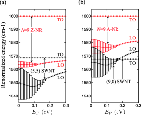
Figure 3: (color online) (a) The $E_{\rm F}$ dependence of the renormalized energies of the LO and TO modes in a $N=9$ Z-NR (red) and of the LO and TO modes in a $(5,5)$ SWNT (black). (b) The $E_{\rm F}$ dependence of the renormalized frequencies of the LO and TO modes in a $N=9$ A-NR (red) and of the LO and TO modes in a $(9,0)$ SWNT (black).

It is noted that, for the renormalized energies of the LO and TO modes in NRs shown in Fig. 3, we have not included all the possible intermediate electron-hole pair states created by a given phonon mode in evaluating $\sum_{\rm eh}$ in Eq. (8). For example, vertical transition denoted by the arrow 3 in Fig. 2(a) may be included as a possible intermediate state in evaluating $\sum_{\rm eh}$ in Eq. (8) although such intermediate state does not satisfy the momentum conservation. In this paper, we do not consider the contribution of momentum non-conserving electron-hole pair creation processes in evaluating $\sum_{\rm eh}$ in Eq. (8).

II.2 Armchair NRs

Next we study the KA in A-NRs. The zigzag SWNTs are cut along their axis and flattened out to make A-NRs. It is known that one third of zigzag SWNTs exhibit a metallic band structure. Saito et al. (1992a) It is interesting to note that if we cut the bonds along the axis of a metallic zigzag SWNT in order to make an A-NR, the obtained A-NR has an energy gap. Namely, unrolling a metallic $(3i,0)$ SWNT results in a $N=3i-1$ A-NR with an energy gap. Instead, unrolling a semiconducting $(3i+1,0)$ SWNT results in a gap-less $N=3i$ A-NR and unrolling a semiconducting $(3i+2,0)$ SWNT results in a $N=3i+1$ A-NR with an energy gap. The one-third periodicity of metallicity is maintained even if zigzag SWNTs are unrolled by cutting the bonds. Since metallicity is a necessary condition for the KA, we study the KA in $N=3i$ metallic A-NRs here.

In order to specify the lattice structure of an A-NR, we use integers $I$ $\in[0,N]$ and $J$ $\in[0,M]$ in Fig. 4(a). In a box specified by $IJ$ in Fig. 4(a), there are two A atoms and two B atoms. For convenience, we divide the two A (B) atoms into up-A (up-B) and down-A (down-B), as shown in Fig. 4(a). The wave function then has four components: $(e^{i(k2\ell)J}/\sqrt{M})(\phi^{I}_{\rm uA},\phi^{I}_{\rm uB},\phi^{I}_{\rm dA},\phi^{I}_{\rm dB})^{t}$ where $k$ is the wave vector along the armchair edge.

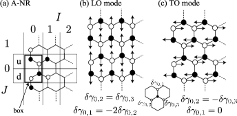
Figure 4: (a) The lattice structure of an A-NR. (b,c) The eigenvectors of the $\Gamma$ point LO and TO phonon modes are illustrated. The LO mode satisfies $\delta\gamma_{0,1}=-2\delta\gamma_{0,2}$ and $\delta\gamma_{0,2}=\delta\gamma_{0,3}$. The TO mode is characterized by $\delta\gamma_{0,1}=0$ and $\delta\gamma_{0,2}=-\delta\gamma_{0,3}$.

In Fig. 4(b) and (c), we show phonon eigenvectors of the $\Gamma$ point LO and TO modes, respectively. The eigenvector of the LO (TO) mode is parallel (perpendicular) to the armchair edge. The LO mode satisfies $\delta\gamma_{0,1}=-2\delta\gamma_{0,2}$ and $\delta\gamma_{0,2}=\delta\gamma_{0,3}$, while the TO mode satisfies $\delta\gamma_{0,1}=0$ and $\delta\gamma_{0,2}=-\delta\gamma_{0,3}$. Since $\delta\gamma_{0,2}$ and $\delta\gamma_{0,3}$ are perturbations that do not mix $\phi_{\rm u}$ and $\phi_{\rm d}$, the electron-hole pair creation matrix element can be divided into the following two parts:

$$\begin{split}&V_{\rm u}=\sum_{I,I^{\prime}}\begin{pmatrix}\phi^{I^{\prime}}_{\rm uA}\cr-\phi^{I^{\prime}}_{\rm uB}\end{pmatrix}^{\dagger}\begin{pmatrix}0&\delta\gamma_{0,3}\delta_{I^{\prime},I}+\delta\gamma_{0,2}\delta_{I^{\prime},I+1}\cr{\rm h.c.}&0\cr\end{pmatrix}\begin{pmatrix}\phi^{I}_{\rm uA}\cr\phi^{I}_{\rm uB}\end{pmatrix},\\ &V_{\rm d}=\sum_{I,I^{\prime}}\begin{pmatrix}\phi^{I^{\prime}}_{\rm dA}\cr-\phi^{I^{\prime}}_{\rm dB}\end{pmatrix}^{\dagger}\begin{pmatrix}0&\delta\gamma_{0,2}\delta_{I^{\prime},I}+\delta\gamma_{0,3}\delta_{I^{\prime},I-1}\cr{\rm h.c.}&0\end{pmatrix}\begin{pmatrix}\phi^{I}_{\rm dA}\cr\phi^{I}_{\rm dB}\end{pmatrix},\end{split}$$ (9)

where the Hermite conjugate (${\rm h.c.}$) of $V_{\rm u}$ ($V_{\rm d}$) is defined as $\delta\gamma_{0,3}\delta_{I^{\prime},I}+\delta\gamma_{0,2}\delta_{I^{\prime},I-1}$ ($\delta\gamma_{0,2}\delta_{I^{\prime},I}+\delta\gamma_{0,3}\delta_{I^{\prime},I+1}$). We can rewrite Eq. (9) as

$$\begin{split}&V_{\rm u}=2i\sum_{I}\left(\delta\gamma_{0,3}{\rm Im}\left[\phi_{\rm uA}^{I*}\phi_{\rm uB}^{I}\right]+\delta\gamma_{0,2}{\rm Im}\left[\phi_{\rm uA}^{I+1*}\phi_{\rm uB}^{I}\right]\right),\\ &V_{\rm d}=2i\sum_{I}\left(\delta\gamma_{0,2}{\rm Im}\left[\phi_{\rm dA}^{I*}\phi_{\rm dB}^{I}\right]+\delta\gamma_{0,3}{\rm Im}\left[\phi_{\rm dA}^{I*}\phi_{\rm dB}^{I+1}\right]\right).\end{split}$$ (10)

The perturbation $\delta\gamma_{0,1}$ mixes $\phi^{I}_{\rm u}$ and $\phi^{I}_{\rm d}$ as

$$U=\sum_{I}\begin{pmatrix}\phi^{I}_{\rm uA}\cr-\phi^{I}_{\rm uB}\cr\phi^{I}_{\rm dA}\cr-\phi^{I}_{\rm dB}\end{pmatrix}^{\dagger}\begin{pmatrix}0&0&0&e^{ik2\ell}\delta\gamma_{0,1}\cr 0&0&\delta\gamma_{0,1}&0\cr 0&\delta\gamma_{0,1}&0&0\cr e^{-ik2\ell}\delta\gamma_{0,1}&0&0&0\end{pmatrix}\begin{pmatrix}\phi^{I}_{\rm uA}\cr\phi^{I}_{\rm uB}\cr\phi^{I}_{\rm dA}\cr\phi^{I}_{\rm dB}\end{pmatrix},$$ (11)

so that $U$ can be rewritten as

$$U=i2\delta\gamma_{0,1}\sum_{I}\left({\rm Im}\left[e^{ik2\ell}\phi^{I*}_{\rm uA}\phi^{I}_{\rm dB}\right]-{\rm Im}\left[\phi^{I*}_{\rm uB}\phi^{I}_{\rm dA}\right]\right).$$ (12)

Now, it can be shown that each energy eigenstate satisfies the following equations (see Appendix A),

$$\begin{split}&\sum_{I}\phi_{\rm uA}^{I*}\phi_{\rm uB}^{I}=\sum_{I}\phi_{\rm dA}^{I*}\phi_{\rm dB}^{I},\\ &\sum_{I}\phi_{\rm uA}^{I+1*}\phi_{\rm uB}^{I}=\sum_{I}\phi_{\rm dA}^{I*}\phi_{\rm dB}^{I+1}.\end{split}$$ (13)

Due to these conditions, the TO mode causes a special cancellation between $V_{\rm u}$ and $V_{\rm d}$ as $V_{\rm u}+V_{\rm d}=0$ since $\delta\gamma_{0,2}+\delta\gamma_{0,3}=0$. In addition, we obtain $U=0$ from $\delta\gamma_{0,1}=0$. Thus the TO modes in A-NRs decouple from electron-hole pairs and do not undergo a KA. For the LO mode, on the other hand, there is no cancellation between $V_{\rm u}$ and $V_{\rm d}$, and the matrix element for the LO mode is given by $V_{\rm L}\equiv U+V_{\rm u}+V_{\rm d}$. By setting $\delta\gamma_{0,2}=\delta\gamma_{0,3}$, $-2\delta\gamma_{0,3}=\delta\gamma$ and $\delta\gamma_{0,1}=\delta\gamma$, we calculate $V_{\rm L}$ and put it into Eq. (8) to obtain $\Pi(\omega_{0})$.

The solid curves in Fig. 3(b) give the $E_{\rm F}$ dependence of the renormalized frequencies $\hbar\omega_{0}+{\rm Re}\left[\Pi(\omega_{0})\right]$ for the LO and TO modes in a $N=9$ A-NR at room temperature. The frequency of the TO mode is given by $\omega_{0}$ showing that the TO mode decouples from electron-hole pairs. The LO mode undergoes a KA. For comparison, we show the renormalized frequency of the LO and TO modes in a $(9,0)$ zigzag SWNT as the black curves in Fig. 3(b). It is found that $|\Pi(\omega_{0})|$ for the LO mode of a $N=9$ A-NR is smaller than $|\Pi(\omega_{0})|$ for the LO mode of a $(9,0)$ zigzag SWNT. It is because there are two linear energy bands near the K and K’ points in metallic zigzag SWNTs, while there is only one linear energy band in metallic A-NRs, and the KAs in A-NRs are suppressed slightly as compared to those in metallic zigzag SWNTs. We note that the broadening in A-NRs is still larger than that in Z-NRs because of the absence of the edge states near the armchair edges. The TO mode of a $(9,0)$ zigzag SWNT is down shifted. However, there is no dependence on $E_{\rm F}$, which indicates that only high energy electron-hole pairs contribute to the self-energy. We will explore the KA effect for the TO mode in zigzag SWNTs in Sec. IV.

We have considered NRs with a long length ($10\mu m$) in calculating the self-energies $\Pi(\omega_{0})$ shown in Fig. 3(a) and (b). For NRs with short lengths, the effect of the level spacing on $\Pi(\omega)$ is not negligible. For example, the level spacing in armchair SWNTs becomes $0.12$eV when $L=30$nm, which is comparable to $\hbar\omega_{0}/2$. Thus the level spacing affects the resonant decay. The effect of the level spacing on the KAs in NRs will be reported elsewhere.

III Raman intensity

III.1 Raman Activity

In the Raman process, an incident photon excites an electron in the valence energy band into a state in the conduction energy band. Then the photo-excited electron emits or absorbs a phonon. The matrix element for the emission or absorption of a phonon is given by the el-ph matrix element for the scattering between an electron state in the conduction energy band and a state in the conduction energy band, which is in contrast to that for the el-ph matrix element for electron-hole pair creation which is relevant to the matrix element from a state in the valence energy band to a state in the conduction energy band. This matrix element for the emission or absorption of a phonon is given by removing the minus sign from $-\phi^{J}_{\rm B}$ (or $-\phi^{I}_{\rm uB,dB}$) of the final state in the electron-hole pair creation matrix elements in Eqs. (1), (9), and (11). This operation is equivalent to replacing ${\rm Im}$ (${\rm Re}$) with ${\rm Re}$ (${\rm Im}$) in Eqs. (3), (4), (10) and (12).

As a result, the Raman intensity of the TO (LO) modes in Z-NRs is proportional to ${\rm Re}\left[\phi^{J*}_{\rm A}\phi^{J}_{\rm B}\right]$ (${\rm Im}\left[\phi^{J*}_{\rm A}\phi^{J}_{\rm B}\right]$). Thus the TO modes are Raman active, while the LO modes are not. Because the TO modes in Z-NRs are free from the KA, the G band Raman spectra exhibit the original frequency of the TO modes, $\hbar\omega_{0}$. For A-NRs, on the other hand, the cancellation between $V_{\rm u}$ and $V_{\rm d}$ occurs for the TO modes, and the TO modes are then not Raman active, while the LO modes are Raman active. Since the LO modes in A-NRs undergo KAs, the renormalized frequencies, $\hbar\omega_{0}+\Pi(\omega_{0})$, will appear below the original frequencies of the LO modes by about 20 cm^-1 (see Fig. 3). Thus, the G band spectra in A-NRs can appear below those in Z-NRs, which is useful in identifying the orientation of the edge of NRs by G band Raman spectroscopy. Our results are summarized in TABLE 1 combined with the results for armchair and zigzag SWNTs.

For the Raman intensity of armchair SWNTs, we obtain the same conclusion as that of Z-NRs, that is, the TO modes are Raman active, while the LO modes are not. For metallic zigzag SWNTs, on the other hand, the cancellation between $V_{\rm u}$ and $V_{\rm d}$ which occurs for the TO modes in A-NRs is not valid. Then the TO modes, in addition to the LO modes, can be Raman active. However, as we will show in Sec. IV, since the matrix element for the emission or absorption of the TO modes vanishes at the van Hove singularities of the electronic sub-bands, then we can conclude that the TO modes are hardly excited in resonant Raman spectroscopy. It is interesting to compare these results with another theoretical results for the Raman intensities of SWNTs. In Ref. Saito et al., 2001, it is shown using bond polarization theory that the Raman intensity is chirality dependent. In particular, for an armchair (zigzag) SWNT, the $A_{1g}$ TO (LO) mode is a Raman active mode, while the $A_{1g}$ LO (TO) mode is not Raman active. These results for SWNTs are consistent with our results. We think that it is natural that the Raman intensity does not change by unrolling the SWNT since the Raman intensity is proportional to the number of carbon atoms in the unit cell and is not sensitive to the small fraction of carbon atoms at the boundary.

Table 1: Dependences of the KAs and Raman intensities on the $\Gamma$ point optical phonon modes in NRs and metallic SWNTs. $\bigcirc$ and $\times$ represent ‘occurrence’ and ‘absence’, respectively. $\triangle$ means that the KA is possible, but the broadening effect weakens due to the presence of the edge states. $\bigtriangledown$ means that the KA is possible, but the $E_{\rm F}$ dependence is suppressed by the decoupling from the metallic energy band crossing at the Dirac point.

	mode	Kohn anomaly	Raman active
Z-NRs	LO	$\triangle$	$\times$
	TO	$\times$	$\bigcirc$
A-NRs	LO	$\bigcirc$	$\bigcirc$
	TO	$\times$	$\times$
Armchair SWNTs	LO	$\bigcirc$	$\times$
(rolled Z-NRs)	TO	$\bigtriangledown$	$\bigcirc$
Zigzag SWNTs	LO	$\bigcirc$	$\bigcirc$
(rolled A-NRs)	TO	$\bigtriangledown$	$\times$

III.2 Comparison With Experiment

We prepare graphene samples by means of the cleavage method to observe the frequency of the G band Raman spectra. In many cases, graphene samples obtained by the cleavage method show that the angles between the edges have an average value equal to multiples of $30^{\circ}$. This is consistent with the results by You et al. You et al. (2008) Figure 5(a) shows an optical image of the exfoliated graphene with the edges crossing each other with an angle of $\sim 30^{\circ}$. This angle can be considered as evidence of the presence of edges composed predominantly of zigzag or armchair edges. Note that, the obtained sample is characterized as a multi-layer graphene. We estimated the number of layers to be about five based on the behavior of the G’ band. The sample is placed on a SiO₂ (100) surface 300 nm in thickness.

The Raman study was performed using a Jobin-Yvon T64000 Raman system. The laser energy is 2.41eV (514.5nm), the laser power is below 1mW and the laser spot is about 1 $\mu m$ in diameter. Figure 5(b) shows spectra for finding the position dependence of the G band. The results show that the G band frequency depends on the position of laser spot. When the spot is focused near the upper edge (A) or far from the edge, the position of the G band is almost similar to that of graphite (1582cm^-1). However, a softening of the G band is clearly seen when the laser spot moves to the vicinity of the lower edge (B).

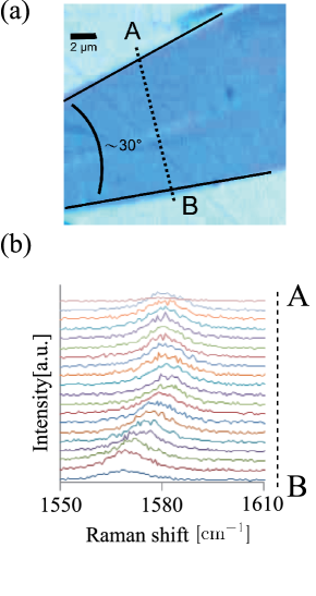
Figure 5: (color online) (a) An optical image of a graphene sample. The sample is characterized as a multi-layer graphene ($\sim$ 5 layers) sample. (b) The position dependence of the G band frequency. From the theoretical results obtained in this paper, we conclude that the G band appearing near the upper (lower) side of the edge consists only of the TO (LO) mode, and that the upper (lower) edge is dominated by the zigzag (armchair) edge.

Based on our theoretical studies, we find that the G band observed near the upper edge consists only of the TO mode, while the G band observed near the lower edge comes from the LO mode, because the G band near the lower edge shows a down shift which is considered to be due to the KA effect of the LO mode. Then, we speculate that the upper (lower) edge is dominated by the zigzag (armchair) edge.

It should be noted that our experiment does not prove that the observed down shift of the G band near the lower edge is due to the KA effect, since we do not examine the $E_{\rm F}$ dependence. There is a possibility that the observed downshift of the G band is related to mechanical effects. Mohiuddin et al. Mohiuddin et al. (2009) observed that the G band splits into two peaks due to uniaxial strain and both peaks exhibit redshifts with increasing strain. The edge in this work somehow has half of it suspended and this may decrease the vibration energy. This effect may explain why for the upper edge in Fig. 5 the frequencies are slightly downshifted compared with the spectra taken at the center of the graphene sample. Moreover, it is probable that the physical edge in this work is a mixture of armchair and zigzag edges. Casiraghi et al. (2009) Note also that we measured the D band in order to confirm that the identification of the orientation of the edge is consistent with the fact that the D band intensity is stronger near the armchair edge than the zigzag edge. Pimenta et al. (2007); You et al. (2008); Malard et al. (2009) However, we could not resolve the difference of the intensity near the upper and lower edges clearly. Zhou et al. Zhou et al. (2008) observed by means of high-resolution angle-resolved photo-emission spectroscopy experiment for epitaxial graphene that the D band gives rise to a kink structure in the electron self-energy and pointed out that an interplay between the el-ph and electron-electron interactions plays an important role in the physics relating to the D band. We will consider these issues further in the future.

IV Pseudospin

In the preceding sections we have shown for Z-NRs that the LO modes are not Raman active and that the TO modes do not undergo KAs. These results originate from the fact that the Bloch function is a real number. Besides, the TO modes in A-NRs are not Raman active and do not undergo KAs. This is due to the cancellation between $V_{\rm u}$ and $V_{\rm d}$ for the TO modes. The LO modes in A-NRs undergo KAs since the Bloch function is a complex number. The absence or presence of a relative phase between the $\phi_{\rm A}$ and $\phi_{\rm B}$ of the Bloch function is essential in deriving our results. In this section, we explain the phase of the Bloch function in terms of the pseudospin, Sasaki and Saito (2008) and clarify the effect of the zigzag and armchair edges on the phase of the Bloch function.

IV.1 Absence of a Pseudospin Phase in Z-NRs

Here we use the effective-mass model in order to understand the reason why the Bloch function in Z-NRs is a real number. In the effective-mass model, the Bloch functions in the conduction energy band near the K and K’ points are given by Sasaki and Saito (2008)

$$\begin{split}&\varphi_{\rm K}(k_{x},k_{y})=\frac{1}{\sqrt{2}}\begin{pmatrix}1\cr e^{i\theta}\end{pmatrix},\\ &\varphi_{\rm K^{\prime}}(k_{x},k_{y})=\frac{1}{\sqrt{2}}\begin{pmatrix}1\cr-e^{-i\theta^{\prime}}\end{pmatrix},\end{split}$$ (14)

where $k_{x}$ and $k_{y}$ ($k^{\prime}_{x}$ and $k^{\prime}_{y}$) are measured from the K (K’) point and the angle $\theta$ ($\theta^{\prime}$) is defined by $k_{x}+ik_{y}\equiv|{\bf k}|e^{i\theta}$ ($k^{\prime}_{x}+ik^{\prime}_{y}\equiv|{\bf k^{\prime}}|e^{i\theta^{\prime}}$). It is noted that $k_{x}$ ($k_{y}$) is taken as parallel to the zigzag (armchair) edge. Then $k_{y}$ is reflected into $-k_{y}$ at the zigzag edge, and the scattered state is given by

$$\varphi_{\rm K}(k_{x},-k_{y})=\frac{1}{\sqrt{2}}\begin{pmatrix}1\cr e^{-i\theta}\end{pmatrix},$$ (15)

as shown in Fig. 6.

Figure 6: In $k$-space, we consider a state near the K point (solid circle) and states which are scattered by the zigzag and armchair edges (empty circles). $k_{x}$ ($k_{y}$) is taken as parallel to the zigzag (armchair) edge. The arrows in the insets indicate the direction of the pseudospins. The $\langle\sigma_{y}\rangle$ component of the pseudospin is reversed at the zigzag edge, while the $\langle\sigma_{x}\rangle$ component is preserved at the armchair edge.

The relative phase of the wave function at the A and B sublattices can be characterized by the direction of the pseudospin. The pseudospin is defined by the expectation value of the Pauli matrices $\sigma_{x,y,z}$ with respect to the Bloch function. Sasaki and Saito (2008) For $\varphi_{\rm K}(k_{x},k_{y})$, we have $\langle\sigma_{x}\rangle=\cos\theta$, $\langle\sigma_{y}\rangle=\sin\theta$, $\langle\sigma_{z}\rangle=0$. For $\varphi_{\rm K}(k_{x},-k_{y})$, we have $\langle\sigma_{x}\rangle=\cos\theta$, $\langle\sigma_{y}\rangle=-\sin\theta$, $\langle\sigma_{z}\rangle=0$. Then $\langle\sigma_{y}\rangle$ flips at the zigzag edge as shown in Fig. 6. Thus, due to an interference between the incoming and reflected waves, we have $\langle\sigma_{y}\rangle=0$ for the Bloch function near the zigzag edge. The condition $\langle\sigma_{y}\rangle=0$ means that the Bloch function becomes a real number. In fact, since $\langle\sigma_{y}\rangle=2\sum_{J}{\rm Im}\left[\phi_{\rm A}^{J*}\phi_{\rm B}^{J}\right]$ and $\langle\sigma_{x}\rangle=2\sum_{J}{\rm Re}\left[\phi_{\rm A}^{J*}\phi_{\rm B}^{J}\right]$ for the Bloch function $(\phi_{\rm A}^{J},\phi_{\rm B}^{J})$ in Eq. (7), the el-ph matrix elements $V_{\rm T}$ and $V_{\rm L}$ (Eq. (3)) are proportional to $\langle\sigma_{y}\rangle$ and $\langle\sigma_{x}\rangle$, respectively. In Appendix B, we show the relationship between the Bloch function $\varphi_{\rm K}$ in the effective-mass model (Eq. (14)) and the Bloch function $(\phi_{\rm A}^{J},\phi_{\rm B}^{J})$ in the tight-binding model (Eq. (7)).

We point out that the condition $\langle\sigma_{y}\rangle=0$ is not satisfied in the case of armchair SWNTs (rolled Z-NRs) except for the lowest energy sub-bands of $k_{y}=0$. This is the reason why we see in Fig. 3(a) that the TO mode exhibits no broadening but a softening with a constant energy $\sim-30$ cm^-1 in a $(5,5)$ SWNT. It is interesting to note that the Aharanov-Bohm flux applied along the tube axis shifts the cutting lines Ajiki and Ando (1993); Zaric et al. (2004); Minot et al. (2004) and can make $k_{y}$ for the lowest energy sub-bands nonzero. Thus the Aharanov-Bohm flux makes that $\langle\sigma_{y}\rangle=\sin\theta\neq 0$ even for the lowest energy sub-bands, for which the TO mode can exhibit a broadening. Ishikawa and Ando (2006)

Since the effective-mass model describes the physics well in the long wave length limit, an advantage in the above discussion of using the effective-mass model is that it is not necessary for the edge of graphene NRs to be well defined on an atomic scale in order that we have a cancellation of $\langle\sigma_{y}\rangle$. This may be a reason why we observe a softening of the G band near the edge of an armchair-rich sample experimentally as shown in Sec. III.2.

IV.2 Coherence of the Pseudospin in A-NRs

On the other hand, a state near the K point with $(k_{x},k_{y})$ is reflected by the armchair edge into a state near the K’ point with $(k^{\prime}_{x},k^{\prime}_{y})=(-k_{x},k_{y})$, and the scattered state is given by $\varphi_{\rm K^{\prime}}(-k_{x},k_{y})$. In this case, by putting $\theta^{\prime}=\pi-\theta$ into $\varphi_{\rm K^{\prime}}(k_{x},k_{y})$ in Eq. (14), we obtain

$$\varphi_{\rm K^{\prime}}(-k_{x},k_{y})=\frac{1}{\sqrt{2}}\begin{pmatrix}1\cr e^{i\theta}\end{pmatrix}$$ (16)

which is identical to the initial Bloch function, $\varphi_{\rm K}(k_{x},k_{y})$. Thus the relative phase between the A and B Bloch functions is conserved thorough the reflection by the armchair edge so that the Bloch function can not be reduced to a real number. Namely, the reflections by the armchair edge preserve the pseudospin as shown in Fig. 6. It is expected that the relative phase makes it possible that KAs occur not only for the LO mode but also for the TO mode near the armchair edge. However, as we have shown in Eq. (13), the armchair edge gives rise to the cancellation between $V_{\rm u}$ and $V_{\rm d}$, so that the TO modes in A-NRs do not undergo KAs. We consider whether Eq. (13) is satisfied in the case of zigzag SWNTs or not, in order to see if the KA effect is present in zigzag SWNTs or not. By applying the Bloch theorem to zigzag SWNTs, we have

$$\begin{split}&\phi_{\rm uA}^{I}=(e^{iIka}/2\sqrt{N})\varphi_{\rm A},\\ &\phi_{\rm uB}^{I}=(e^{i(I+1/2)ka}/2\sqrt{N})\varphi_{\rm B},\\ &\phi_{\rm dA}^{I}=(e^{i(I+1/2)ka}/2\sqrt{N})\varphi_{\rm A},\\ &\phi_{\rm dB}^{I}=(e^{iIka}/2\sqrt{N})\varphi_{\rm B},\end{split}$$ (17)

where we set $\varphi_{\phi}={}^{t}(\varphi_{\rm A},\varphi_{\rm B})$. Using these equations, we obtain

$$\begin{split}&\sum_{I}\phi_{\rm uA}^{I*}\phi_{\rm uB}^{I}=\frac{1}{4}e^{i\frac{ka}{2}}\varphi_{\rm A}^{*}\varphi_{\rm B},\\ &\sum_{I}\phi_{\rm dA}^{I*}\phi_{\rm dB}^{I}=\frac{1}{4}e^{-i\frac{ka}{2}}\varphi_{\rm A}^{*}\varphi_{\rm B}.\end{split}$$ (18)

Thus the first equation in Eq. (13) is not satisfied for zigzag SWNTs. Similarly, we have

$$\begin{split}&\sum_{I}\phi_{\rm uA}^{I+1*}\phi_{\rm uB}^{I}=\frac{1}{4}e^{-i\frac{ka}{2}}\varphi_{\rm A}^{*}\varphi_{\rm B},\\ &\sum_{I}\phi_{\rm dA}^{I*}\phi_{\rm dB}^{I+1}=\frac{1}{4}e^{i\frac{ka}{2}}\varphi_{\rm A}^{*}\varphi_{\rm B},\end{split}$$ (19)

which shows that the second equation in Eq. (13) is not fulfilled, either. Thus the TO modes can undergo KAs because the cancellation between $V_{\rm u}$ and $V_{\rm d}$ is not possible for zigzag SWNTs. In fact, by putting Eqs. (18) and (19) into Eq. (10), we get

$$V_{\rm u}+V_{\rm d} =i(\delta\gamma_{0,2}+\delta\gamma_{0,3})\sin\theta\cos\frac{ka}{2}$$

$$+i(\delta\gamma_{0,3}-\delta\gamma_{0,2})\cos\theta\sin\frac{ka}{2},$$ (20)

where we set $\varphi_{\rm A}^{*}\varphi_{\rm B}=e^{i\theta}$. Because the TO modes satisfy $\delta\gamma_{0,2}+\delta\gamma_{0,3}=0$, $V_{\rm u}+V_{\rm d}$ can take a nonzero value for

$$V_{\rm u}+V_{\rm d}=i2\delta\gamma_{0,3}\sin\left(\frac{ka}{2}\right)\cos\theta.$$ (21)

It is noted that Eq. (21) vanishes when $\theta=\pm\pi/2$. This condition $\theta=\pm\pi/2$ is satisfied for low energy electron-hole pairs when the energy band crosses the Dirac point. In other words, high energy electron-hole pairs in the sub-bands can contribute to a frequency softening of the TO mode in zigzag SWNTs. This is why we obtain the down shift of the TO mode for a $(9,0)$ zigzag SWNT as shown in Fig. 3. In “metallic” zigzag SWNTs, the curvature effect shifts the position of the cutting line Saito et al. (2005) of the metallic energy band from the Dirac point and produces a small energy gap. Saito et al. (1992b); Kane and Mele (1997); Ando (2000); Yang and Han (2000) In this case, the low energy electron-hole pairs satisfy $\cos\theta\neq 0$ in Eq. (21) and they contribute to a frequency hardening of the TO modes in metallic zigzag SWNTs. The curvature effect gives rise to a change of the Fermi surface and results in KAs for the TO modes. Sasaki et al. (2008a)

Similarly, the matrix element for the emission or absorption of the TO modes in zigzag SWNTs is given by

$$2\delta\gamma_{0,3}\sin\left(\frac{ka}{2}\right)\sin\theta,$$ (22)

which does not vanish in general. This shows that the TO modes in zigzag SWNTs can be Raman active. However, since the van Hove singularities of sub-bands in zigzag SWNTs are located on the $k_{x}$ axis (and satisfy $\theta=0$), the $\sin\theta$ factor tells us that the TO modes are hardly excited in resonant Raman spectroscopy.

V Discussion

The theoretical analysis performed in this paper is based on the use of a simple tight-binding method which includes only the first nearest-neighbor hopping integral and its variation due to the atomic displacements. The approximation used is partly justified because the deformation-potential and the el-ph matrix element with respect to the second nearest-neighbors is about one order of magnitude smaller than that of the first nearest neighbors. Porezag et al. (1995); Jiang et al. (2005) However, we have not considered the effect of the overlap integral. The overlap integral breaks the particle-hole symmetry and may invalidate our results. Besides, we have neglected the contribution of momentum non-conserving electron-hole pair creation processes in evaluating $\sum_{\rm eh}$ in Eq. (8). Although this is an approximation which works well for thin NRs, the inclusion of the momentum non-conserving electron-hole pair creation processes may invalidate our results. We will elaborate on this idea in the future.

VI Summary

In summary, the LO modes undergo KAs in graphene NRs while the TO modes do not. This conclusion does not depend on the orientation of the edge. In Z-NRs, the Raman intensities of the LO modes are strongly suppressed because the wave function is a real number, and only the TO modes are Raman active. As a result, the KA for the LO mode in Z-NRs would be difficult to observe in Raman spectroscopy. In A-NRs, only the LO modes are Raman active owing to the cancellation between $V_{\rm u}$ and $V_{\rm d}$. The “chirality” dependent Raman intensity derived for NRs is the same as the chirality dependent Raman intensity for SWNTs calculated in Ref. Saito et al., 2001. The strong down shift of the LO mode makes it possible to identify the orientation of edges of graphene by the G band Raman spectroscopy due to the “chirality” dependent Raman intensity.

Appendix A Derivation of Eq. (13)

In this Appendix, we derive Eq. (13) by using mirror and time-reversal symmetries. Let us introduce the mirror-reflection operator $M$ by

$$M\phi^{I}_{n,k}=\begin{pmatrix}0&0&0&1\cr 0&0&1&0\cr 0&1&0&0\cr 1&0&0&0\end{pmatrix}\begin{pmatrix}\phi^{I}_{\rm uA}\cr\phi^{I}_{\rm uB}\cr\phi^{I}_{\rm dA}\cr\phi^{I}_{\rm dB}\end{pmatrix}\ \ (I=0,\ldots,N),$$ (23)

where $k$ is the wave vector along the armchair edge and $n$ is the band index. By applying $M$ to the energy eigen-equation $H_{k}\phi_{n,k}=E_{n,k}\phi_{n,k}$, we get $MH_{k}\phi_{n,k}=E_{n,k}M\phi_{n,k}$. Since the Hamiltonian satisfies $MH_{k}M^{-1}=H_{-k}$, we obtain $M\phi_{n,k}=e^{i\phi}\phi_{n,-k}$ where $\phi$ is a phase factor.

On the other hand, due to the time-reversal symmetry, we have $\phi_{n,k}^{*}=e^{i\phi^{\prime}}\phi_{n,-k}$. Thus, by combing the time-reversal symmetry ($\phi_{n,k}^{*}=e^{i\phi^{\prime}}\phi_{n,-k}$) with the mirror symmetry ($M\phi_{n,k}=e^{i\phi}\phi_{n,-k}$), we get

$$M\phi_{n,k}=e^{i\phi^{\prime\prime}}\phi_{n,k}^{*},$$ (24)

that is,

$$\begin{pmatrix}\phi^{I}_{\rm dB}\cr\phi^{I}_{\rm dA}\cr\phi^{I}_{\rm uB}\cr\phi^{I}_{\rm uA}\end{pmatrix}=e^{i\phi^{\prime\prime}}\begin{pmatrix}\phi^{I*}_{\rm uA}\cr\phi^{I*}_{\rm uB}\cr\phi^{I*}_{\rm dA}\cr\phi^{I*}_{\rm dB}\end{pmatrix}.$$ (25)

Using this condition, one sees that Eq. (13) is satisfied.

Appendix B Relationship between Eq. (7) and Eq. (14)

Here we will show for Z-NRs that the Bloch function derived using the tight-binding lattice model (Eq. (7)) is a superposition of incoming and reflected Bloch functions derived using the effective-mass model (Eq. (14)).

By rewriting the Bloch function of Z-NRs $(\phi_{\rm A}^{J},\phi_{\rm B}^{J})$ in Eq. (7) as

$$\begin{split}&\phi_{\rm A}^{J}=\frac{C(g,\phi)}{2i}\left(\frac{1}{g}+e^{i\phi}\right)e^{iJ\phi}+{\rm c.c.},\\ &\phi_{\rm B}^{J}=\frac{C(g,\phi)}{2i}\epsilon(g,\phi)\frac{e^{i\phi}}{g}e^{iJ\phi}+{\rm c.c.},\end{split}$$ (26)

where ${\rm c.c.}$ denotes the complex conjugation of the first term, one sees that $(\phi_{\rm A}^{J},\phi_{\rm B}^{J})$ is a real number as a result of the cancellation of the imaginary part between the first and second terms. By introducing a new Bloch function $\varphi_{\phi}$ as

$$\varphi_{\phi}\equiv\frac{C(g,\phi)}{2ig}e^{i\phi}\begin{pmatrix}g+e^{-i\phi}\cr\epsilon(g,\phi)\end{pmatrix},$$ (27)

the Bloch function $(\phi_{\rm A}^{J},\phi_{\rm B}^{J})$ is expressed by

$$\begin{pmatrix}\phi_{\rm A}^{J}\cr\phi_{\rm B}^{J}\end{pmatrix}=\varphi_{\phi}e^{iJ\phi}+\varphi_{\phi}^{*}e^{-iJ\phi}.$$ (28)

Because of the different signs in the exponents of $e^{iJ\phi}$ and $e^{-iJ\phi}$ in Eq. (28), $\phi$ may be thought of as the wave vector perpendicular to the zigzag edge ($k_{y}$) multiplied by a lattice constant ($\ell$) as $\phi=k_{y}\ell$. Assuming that $\phi=k_{y}\ell$, the zigzag edge reflects a state with $k_{y}$ ($\varphi_{\phi}e^{iJ\phi}$) into a state with $-k_{y}$ ($\varphi_{-\phi}e^{-iJ\phi}$). We then expect that the Bloch function near the zigzag edge is given by

$$\varphi_{\phi}e^{iJ\phi}+\varphi_{-\phi}e^{-iJ\phi}.$$ (29)

It is noted that Eq. (29) is different from Eq. (28) because $\varphi_{-\phi}$ is not identical to $\varphi_{\phi}^{*}$ in general. However, we will get $\varphi_{-\phi}=\varphi_{\phi}^{*}$ for Z-NRs because we may assume that the normalization constant $C(g,\phi)$ in Eq. (27) satisfies $C(g,-\phi)=-C^{*}(g,\phi)$ without loss of generality. Therefore, Eq. (29) is consistent to Eq. (28), which indicates that the assumption ($\phi=k_{y}\ell$) is appropriate. The condition $\varphi_{-\phi}=\varphi_{\phi}^{*}$ is a non-trivial condition since it is satisfied only for the zigzag edge and is essential for $(\phi_{\rm A}^{J},\phi_{\rm B}^{J})$ to be a real number.

Using Eq. (14) we obtain $\varphi_{\rm K}(k_{x},-k_{y})=\varphi_{\rm K}(k_{x},k_{y})^{*}$ which corresponds to $\varphi_{-\phi}=\varphi_{\phi}^{*}$. In fact, by putting $(g+e^{-i\phi})\equiv|g+e^{-i\phi}|e^{-i\Theta}$ into Eq. (27) and by using $\epsilon(g,\phi)=|g+e^{-i\phi}|$, Sasaki et al. (2005) the Bloch state $\varphi_{\phi}$ can be written as

$$\varphi_{\phi}=\frac{1}{\sqrt{2}}\begin{pmatrix}1\cr e^{i\Theta}\end{pmatrix},$$ (30)

where $\Theta$ and $\theta$ are the same as each other near the K point.

References

- Li et al. (2008) X. Li, X. Wang, L. Zhang, S. Lee, and H. Dai, Science 319, 1229 (2008).
- Jiao et al. (2009) L. Jiao, L. Zhang, X. Wang, G. Diankov, and H. Dai, Nature 458, 877 (2009).
- Kosynkin et al. (2009) D. V. Kosynkin, A. L. Higginbotham, A. Sinitskii, J. R. Lomeda, A. Dimiev, B. K. Price, and J. M. Tour, Nature 458, 872 (2009).
- Saito et al. (1992a) R. Saito, M. Fujita, G. Dresselhaus, and M. S. Dresselhaus, Appl. Phys. Lett. 60, 2204 (1992a).
- Liu et al. (2009) Z. Liu, K. Suenaga, P. J. F. Harris, and S. Iijima, Phys. Rev. Lett. 102, 015501 (2009).
- Jia et al. (2009) X. Jia, M. Hofmann, V. Meunier, B. G. Sumpter, J. Campos-Delgado, J. M. Romo-Herrera, H. Son, Y.-P. Hsieh, A. Reina, J. Kong, et al., Science 323, 1701 (2009).
- Girit et al. (2009) C. O. Girit, J. C. Meyer, R. Erni, M. D. Rossell, C. Kisielowski, L. Yang, C.-H. Park, M. F. Crommie, M. L. Cohen, S. G. Louie, et al., Science 323, 1705 (2009).
- Kobayashi (1993) K. Kobayashi, Phys. Rev. B 48, 1757 (1993).
- Fujita et al. (1996) M. Fujita, K. Wakabayashi, K. Nakada, and K. Kusakabe, J. Phys. Soc. Jpn. 65, 1920 (1996).
- Nakada et al. (1996) K. Nakada, M. Fujita, G. Dresselhaus, and M. S. Dresselhaus, Phys. Rev. B 54, 17954 (1996).
- Wakabayashi et al. (1999) K. Wakabayashi, M. Fujita, H. Ajiki, and M. Sigrist, Phys. Rev. B 59, 8271 (1999).
- Holden et al. (1994) J. M. Holden, P. Zhou, X.-X. Bi, P. C. Eklund, S. Bandow, R. A. Jishi, K. D. Chowdhury, G. Dresselhaus, and M. S. Dresselhaus, Chem. Phys. Lett. 220, 186 (1994).
- Rao et al. (1997) A. M. Rao, E. Richter, S. Bandow, B. Chase, P. C. Eklund, K. W. Williams, S. Fang, K. R. Subbaswamy, M. Menon, A. Thess, et al., Science 275, 187 (1997).
- Sugano et al. (1998) M. Sugano, A. Kasuya, K. Tohji, Y. Saito, and Y. Nishina, Chem. Phys. Lett. 292, 575 (1998).
- Pimenta et al. (1998) M. A. Pimenta, A. Marucci, S. A. Empedocles, M. G. Bawendi, E. B. Hanlon, A. M. Rao, P. C. Eklund, R. E. Smalley, G. Dresselhaus, and M. S. Dresselhaus, Phys. Rev. B 58, R16016 (1998).
- Yu and Brus (2001) Z. Yu and L. Brus, J. Phys. Chem. B 105, 1123 (2001).
- Jorio et al. (2001) A. Jorio, R. Saito, J. H. Hafner, C. M. Lieber, M. Hunter, T. McClure, G. Dresselhaus, and M. S. Dresselhaus, Phys. Rev. Lett. 86, 1118 (2001).
- Bachilo et al. (2002) S. Bachilo, M. Strano, C. Kittrell, R. Hauge, R. Smalley, and R. Weisman, Science 298, 2361 (2002).
- Strano et al. (2003) M. Strano, S. Doorn, E. Haroz, C. Kittrell, R. Hauge, and R. Smalley, Nano Letters 3, 1091 (2003).
- Doorn et al. (2004) S. Doorn, D. Heller, P. Barone, M. Usrey, and M. Strano, Appl. Phys. A: Mater. Sci. Process. 78, 1147 (2004).
- Dresselhaus et al. (2005) M. S. Dresselhaus, G. Dresselhaus, R. Saito, and A. Jorio, Physics Reports 409, 47 (2005).
- Cançado et al. (2004) L. G. Cançado, M. A. Pimenta, B. R. A. Neves, G. Medeiros-Ribeiro, T. Enoki, Y. Kobayashi, K. Takai, K.-i. Fukui, M. S. Dresselhaus, R. Saito, et al., Phys. Rev. Lett. 93, 47403 (2004).
- Ferrari et al. (2006) A. C. Ferrari, J. C. Meyer, V. Scardaci, C. Casiraghi, M. Lazzeri, F. Mauri, S. Piscanec, D. Jiang, K. S. Novoselov, S. Roth, et al., Phys. Rev. Lett. 97, 187401 (2006).
- Yan et al. (2007) J. Yan, Y. Zhang, P. Kim, and A. Pinczuk, Phy. Rev. Lett. 98, 166802 (2007).
- Pimenta et al. (2007) M. A. Pimenta, G. Dresselhaus, M. S. Dresselhaus, L. G. Cancado, A. Jorio, and R. Saito, Phys. Chem. Chem. Phys. 9, 1276 (2007).
- Casiraghi et al. (2009) C. Casiraghi, A. Hartschuh, H. Qian, S. Piscanec, C. Georgi, A. Fasoli, K. S. Novoselov, D. M. Basko, and A. C. Ferrari, Nano Letters 9, 1433 (2009).
- Malard et al. (2009) L. Malard, M. Pimenta, G. Dresselhaus, and M. Dresselhaus, Physics Reports 473, 51 (2009), ISSN 0370-1573.
- Farhat et al. (2007) H. Farhat, H. Son, G. G. Samsonidze, S. Reich, M. S. Dresselhaus, and J. Kong, Phys. Rev. Lett. 99, 145506 (2007).
- Nguyen et al. (2007) K. T. Nguyen, A. Gaur, and M. Shim, Phys. Rev. Lett. 98, 145504 (2007).
- Wu et al. (2007) Y. Wu, J. Maultzsch, E. Knoesel, B. Chandra, M. Huang, M. Y. Sfeir, L. E. Brus, J. Hone, and T. F. Heinz, Phys. Rev. Lett. 99, 027402 (2007).
- Das et al. (2007) A. Das, A. K. Sood, A. Govindaraj, A. M. Saitta, M. Lazzeri, F. Mauri, and C. N. R. Rao, Phys. Rev. Lett. 99, 136803 (2007).
- Kohn (1959) W. Kohn, Phys. Rev. Lett. 2, 393 (1959).
- Dubay et al. (2002) O. Dubay, G. Kresse, and H. Kuzmany, Phys. Rev. Lett. 88, 235506 (2002).
- Piscanec et al. (2004) S. Piscanec, M. Lazzeri, F. Mauri, A. C. Ferrari, and J. Robertson, Phys. Rev. Lett. 93, 185503 (2004).
- Lazzeri and Mauri (2006) M. Lazzeri and F. Mauri, Phys. Rev. Lett. 97, 266407 (2006).
- Piscanec et al. (2007) S. Piscanec, M. Lazzeri, J. Robertson, A. C. Ferrari, and F. Mauri, Phys. Rev. B 75, 035427 (2007).
- Caudal et al. (2007) N. Caudal, A. M. Saitta, M. Lazzeri, and F. Mauri, Phy. Rev. B 75, 115423 (2007).
- Pisana et al. (2007) S. Pisana, M. Lazzeri, C. Casiraghi, K. S. Novoselov, A. K. Geim, A. C. Ferrari, and F. Mauri, Nature Materials 6, 198 (2007).
- Ando (2008) T. Ando, J. Phys. Soc. Jpn. 77, 014707 (2008).
- Sasaki et al. (2008a) K. Sasaki, R. Saito, G. Dresselhaus, M. S. Dresselhaus, H. Farhat, and J. Kong, Phys. Rev. B 77, 245441 (2008a).
- You et al. (2008) Y. You, Z. Ni, T. Yu, and Z. Shen, Applied Physics Letters 93, 163112 (2008).
- Saito et al. (1998) R. Saito, G. Dresselhaus, and M. Dresselhaus, Physical Properties of Carbon Nanotubes (Imperial College Press, London, 1998).
- Sasaki et al. (2006) K. Sasaki, S. Murakami, and R. Saito, J. Phys. Soc. Jpn. 75, 074713 (2006).
- Sasaki et al. (2005) K. Sasaki, S. Murakami, R. Saito, and Y. Kawazoe, Phys. Rev. B 71, 195401 (2005).
- Jiang et al. (2005) J. Jiang, R. Saito, G. G. Samsonidze, S. G. Chou, A. Jorio, G. Dresselhaus, and M. S. Dresselhaus, Phys. Rev. B 72, 235408 (2005).
- Porezag et al. (1995) D. Porezag, T. Frauenheim, T. Köhler, G. Seifert, and R. Kaschner, Phys. Rev. B 51, 12947 (1995).
- Sasaki et al. (2008b) K. Sasaki, R. Saito, G. Dresselhaus, M. S. Dresselhaus, H. Farhat, and J. Kong, Phys. Rev. B 78, 235405 (2008b).
- Saito et al. (2001) R. Saito, A. Jorio, J. H. Hafner, C. M. Lieber, M. Hunter, T. McClure, G. Dresselhaus, and M. S. Dresselhaus, Phys. Rev. B 64, 085312 (2001).
- Mohiuddin et al. (2009) T. M. G. Mohiuddin, A. Lombardo, R. R. Nair, A. Bonetti, G. Savini, R. Jalil, N. Bonini, D. M. Basko, C. Galiotis, N. Marzari, et al., Phys. Rev. B 79, 205433 (2009).
- Zhou et al. (2008) S. Y. Zhou, D. A. Siegel, A. V. Fedorov, and A. Lanzara, Phys. Rev. B 78, 193404 (2008).
- Sasaki and Saito (2008) K. Sasaki and R. Saito, Prog. Theor. Phys. Suppl. 176, 253 (2008).
- Ajiki and Ando (1993) H. Ajiki and T. Ando, J. Phys. Soc. Jpn. 62, 2470 (1993).
- Zaric et al. (2004) S. Zaric, G. N. Ostojic, J. Kono, J. Shaver, V. C. Moore, M. S. Strano, R. H. Hauge, R. E. Smalley, and X. Wei, Science 304, 1129 (2004).
- Minot et al. (2004) E. D. Minot, Y. Yaish, V. Sazonova, and P. L. McEuen, Nature 428, 536 (2004).
- Ishikawa and Ando (2006) K. Ishikawa and T. Ando, J. Phys. Soc. Jpn. 75, 084713 (2006).
- Saito et al. (2005) R. Saito, K. Sato, Y. Oyama, J. Jiang, G. G. Samsonidze, G. Dresselhaus, and M. S. Dresselhaus, Phys. Rev. B 72, 153413 (2005).
- Saito et al. (1992b) R. Saito, M. Fujita, G. Dresselhaus, and M. S. Dresselhaus, Phys. Rev. B 46, 1804 (1992b).
- Kane and Mele (1997) C. L. Kane and E. J. Mele, Phys. Rev. Lett. 78, 1932 (1997).
- Ando (2000) T. Ando, J. Phys. Soc. Jpn. 69, 1757 (2000).
- Yang and Han (2000) L. Yang and J. Han, Phys. Rev. Lett. 85, 154 (2000).