First order non-equilibrium phase transition and bistability of an electron gas

Abstract

We study the carrier concentration bistabilities that occur to a highly photo-excited electron gas. The kinetics of this non-equilibrium electron gas is given by a set of nonlinear rate equations. For low temperatures and cw photo-excitation we show that they have three steady state solutions when the photo-excitation energy is in a certain interval which depends on the electron-electron interaction. Two of them are stable and the other is unstable. We also find the hysteresis region in terms of which these bistabilities are expressed. A diffusion model is constructed which allows the coexistence of two homogeneous spatially separated phases in the non-equilibrium electron gas. The order parameter is the difference of the electron population in the bottom of the conduction band of these two steady stable states. By defining a generalized free potential we obtain the Maxwell construction that determines the order parameter. This order parameter goes to zero when we approach to the critical curve. Hence, this phase transition is a non-equilibrium first order phase transition.

Keywords: non-equilibrium phase transition; bistability; non-linear rate equations; semiconductor electron gas.

Estudiamos las biestabilidades en la concentración de portadores que le ocurren a un gas de electrones altamente fotoexcitado. La cinética de este gas de electrones fuera de equilibrio está dada por un conjunto de ecuaciones de razón no-lineales. Para bajas temperaturas y fotoexcitación en modo continuo (cw) mostramos que estas ecuaciones tienen tres soluciones de estado estacionario cuando la energía de fotoexcitación está en un cierto intervalo, el cual depende de la interacción electrón-electrón. Dos de ellas son estables y la otra es inestable. También, encontramos la región de histeresis en términos de la cual estas biestabilidades son expresadas. Construimos un modelo de difusión que permite la coexistencia de dos fases homogéneas espacialmente separadas del gas de electrones fuera de equilibrio. El parámetro de orden es la diferencia de la población electrónica en el fondo de la banda de conducción de estos dos estados estacionarios estables. Definiendo un potencial libre generalizado del sistema obtenemos la construcción de Maxwell que determina entonces al parámetro de orden. El parámetro de orden va a cero cuando nos aproximamos a la curva crítica. Por eso, esta transición de fase es una transición de fase fuera de equilibrio de primer orden.

Descriptores: transición de fase fuera de equilibrio; biestabilidad; ecuaciones de razón no-lineales; gas de electrones en semiconductores.

I Introduction

Bistability, threshold switching transitions, spatial pattern formation, self-sustained oscillations and chaos in semiconductors are related to non-equilibrium phase transitionsscholl2007 ; scholl . These non-equilibrium phase transitions in semiconductors have been studied in the past decades mainly in connection with the nonlinear generation-recombination mechanism, including impact ionizationscholl ; landsberg76 ; pimpale . Optical and transport properties of semiconductors strongly depend on the electron population in the bottom of the conduction band and many experimental and theoretical studies on hot photo excited electron systems have shown that this electron population depends on the excitation energyhotel ; shah ; carrillo . In this paper we present a study of the carrier concentration bistability that occur to an electron gas generated by a laser excitation and a study of a first order non-equilibrium phase transition between two homogeneous stable steady states of the excited electron gas. They both appear when the energy of the pump is varied. The order parameter is the difference between the electron populations in the bottom of the conduction band of the stable states. It depends upon the effectiveness of the electron-electron interaction. We obtain the order parameter by defining a potential which allows us to make a construction similar to the Maxwell construction for the equilibrium phase transition of a van der Waals gasschlogl ; mar2001 .

In following section we present the theoretical model we use to study a non-equilibrium electron gas in semiconductors. In section third we deduce the stationary state solutions to the non-linear rate equations of the model and we make the estability analysis. By considering a standard first order phase transition of the classical van der Waals gas, we analyze the non-equilibrium phase transition of the electron gas and obtain the corresponding Maxwell construction. We draw our conclusion in the final section.

II Theoretical model of the non-equilibrium electron gas

We describe the non-equilibrium electron gas in semiconductors using the model equations given in Ref. mar . Here, we give a brief description of these model equations and refer the reader to the details of their derivation to Refs. mar2001 ; mar . Electrons in the bottom of the conduction band of a semiconductor play an important role in the dynamics of the whole conduction electron gas. In general, electrons with an energy in excess less than the longitudinal optical (LO) phonon energy can not make transitions by emitting LO phonons. In the case in which the emission of LO phonons is one of the dominant mechanisms, the nonequilibrium kinetics of the electron gas in the conduction band of a semiconductor is given as followsmar . We define a set of energy levels, each one of them representing an energy interval of width $\Delta\epsilon$ of the conduction band. Although not strictly necessary, for simplicity $\Delta\epsilon$ is set equal to $\hbar\omega_{\mbox{\scriptsize LO}}$, the LO phonon energymar . We set the electron population $\chi_{i}$ in these energy levels and, based on the main interaction mechanisms, the nonlinear rate equations that give the temporal behavior of these populations are obtained.

When an electron in level $i$ emits a LO phonon it losses an amount of energy $\hbar\omega_{\mbox{\scriptsize LO}}$ and passes to the level $i-1$. If the frequency of this event is $\nu_{o}^{+}$ then we have that the rate of change of population $\chi_{i}$ is $\nu_{o}^{+}(\chi_{i+1}-\chi_{i})$. Similarly for the absorpion of a LO phonon we have the rate $\nu_{o}^{-}(\chi_{i-1}-\chi_{i})$ where $\nu_{o}^{-}$ is the frequency of this process. The electron-electron interaction gives to the rate of change of the population $\chi_{i}$ at level $i$ two terms, $ZN_{{\mbox{\scriptsize max}}}\chi_{\mbox{\scriptsize tot}}(\chi_{i+1}-2\chi_{i}+\chi_{i-1})$ and $ZN_{{\mbox{\scriptsize max}}}\chi_{0}(\chi_{i}-\chi_{i-1})$. Their form come from considering the contribution to the rate of change of the population $\chi_{i}$ of the interaction between electron populations of all the energy levels, and from the use of energy conservationmar . When an electron suffers a recombination it returns to the valence band and this gives us the term $-w\chi_{i}$ with $w$ the frequency of the process.

Then, by collecting all these contributions, we have the following set of rate equations which describes the kinetics of a photo-excited electron gas in semiconductorsmar ,

$$\frac{d\chi_{i}}{dt} = \nu_{o}^{+}(\chi_{i+1}-\chi_{i})+\nu_{o}^{-}(\chi_{i-1}-\chi_{i})$$ (1)

$$+ZN_{{\mbox{\scriptsize max}}}\chi_{\mbox{\scriptsize tot}}(\chi_{i+1}-2\chi_{i}+\chi_{i-1})$$

$$+ZN_{{\mbox{\scriptsize max}}}\chi_{0}(\chi_{i}-\chi_{i-1})+g_{p}\delta_{i,i_{p}}-w\chi_{i}\quad,$$

for $i\neq 0$. For $i=0$, since the emission of LO phonons by an electron is not possible, we have

$$\frac{d\chi_{0}}{dt} = \nu_{o}^{+}\chi_{1}-\nu_{o}^{-}\chi_{0}+ZN_{{\mbox{\scriptsize max}}}\chi_{\mbox{\scriptsize tot}}(\chi_{1}-\chi_{0})$$ (2)

$$+ZN_{{\mbox{\scriptsize max}}}\chi_{0}\chi_{0}+g_{p}\delta_{0,i_{p}}-w\chi_{0}\quad.$$

The electron populations $\chi_{i}$ have been normalized to the maximum reachable electron concentration $N_{{\mbox{\scriptsize max}}}$ and $\chi_{\mbox{\scriptsize tot}}=\sum\chi_{i}$. The terms with the Kronecker delta is the generation contribution with generation rate $g_{p}$. The main interaction mechanisms, the generation and recombination terms depend on the lattice temperature, carrier concentration and material parameters.

Due to the electron-electron interaction, this set of rate equations is non linear. We should say that Eqs. (1) and (2) which are the main equations of our model came from a more general theory published in Ref. mar . See, also Refs. carrillo ; mar2001 ; lilia for other details of the model equations and other applications.

We make the following definitions $\nu\equiv\nu_{\mbox{\scriptsize o}}^{+}/ZN_{\mbox{\scriptsize max}}$, $\mu\equiv\nu_{\mbox{\scriptsize o}}^{-}/ZN_{\mbox{\scriptsize max}}$, $\omega\equiv w/ZN_{\mbox{\scriptsize max}}$, $\chi_{p}\equiv g_{p}/ZN_{\mbox{\scriptsize max}}$, and $\varepsilon\equiv\epsilon/\Delta\epsilon$. By this normalization, we have eliminated one parameter. For low temperaturesmar , $\mu\ll\nu$. Also, in steady state, $\chi_{p}=\omega$, $\chi_{\mbox{\scriptsize tot}}=1$ and the total carrier concentration $N=N_{\mbox{\scriptsize max}}$. Hence, in this case, we have only two relevant control parameters, $\nu$ and $\varepsilon_{p}$. Here $\varepsilon_{p}=\epsilon_{p}/\Delta\epsilon$, the excitation energy in units of $\Delta$$\epsilon$.

With these definitions and assumptions and considering the finite differences as derivatives:

$$\chi_{i+1}-\chi_{i} \rightarrow \frac{d\chi}{d\epsilon}\Delta\epsilon$$

$$\chi_{i+1}-2\chi_{i}+\chi_{i-1} \rightarrow \frac{d^{2}\chi}{d\epsilon^{2}}(\Delta\epsilon)^{2}$$

$$\chi_{i}-\chi_{i-1} \rightarrow \frac{d\chi}{d\epsilon}\Delta\epsilon-\frac{d^{2}\chi}{d\epsilon^{2}}(\Delta\epsilon)^{2}$$

we have that the equations (1) and (2) that give the steady state of a cw photo-excited electron gas in semiconductors are translated to the following differential equation

$$0=(1-\chi_{0})\frac{d^{2}\chi}{d\varepsilon^{2}}+(\nu+\chi_{0})\frac{d\chi}{d\varepsilon}+\omega\delta(\varepsilon-\varepsilon_{p})-\omega\chi$$ (3)

The electron distribution function $\chi(\varepsilon,\tau)$ is continuous and positive definite in the whole interval $0\leq\varepsilon<\infty$ and has a discontinuity in its first derivative at $\varepsilon=\varepsilon_{p}$. In addition, it must satisfy the conditions

$$\chi_{\mbox{\scriptsize tot}} = \int_{0}^{\infty}d\varepsilon\;\chi(\varepsilon,\tau)$$ (4)

$$\chi_{0} = \int_{0}^{1}d\varepsilon\;\chi(\varepsilon,\tau)$$ (5)

The Eq. (3) has the steady state solutioncarrillo

$$\chi^{s}(\varepsilon)=\left\{\begin{array}[]{lll}Ae^{\alpha\varepsilon}+Be^{-\beta\varepsilon}&;&0\leq\varepsilon\leq\varepsilon_{p}\\ Ce^{-\beta\varepsilon}&;&\varepsilon_{p}\leq\varepsilon\end{array}\right.$$

where

$$\left.\begin{array}[]{l}\alpha\\ \beta\end{array}\right\}=\frac{\left[(\nu+\chi_{0}^{s})^{2}+4\omega(1-\chi_{0}^{s})\right]^{1/2}\mp(\nu+\chi_{0}^{s})}{2(1-\chi_{0}^{s})}$$ (6)

The electron population at the lowest level $\chi_{0}^{s}$ is determined self-consistently by the equation

$$\chi_{0}^{s}=\frac{\omega}{\alpha}e^{-\alpha\varepsilon_{p}}\frac{e^{\alpha}-e^{-\beta}}{\alpha+\beta}\frac{1}{1-\chi_{0}^{s}}$$ (7)

The coefficients $A$, $B$, and $C$ are obtained using the continuity in $\chi(\varepsilon)$, the discontinuity in its first derivative at $\varepsilon=\varepsilon_{p}$, and Eq. (4). In particular, we obtain that $A/B=\alpha/\beta$ (See Ref. carrillo for more details).

To conclude this section we give the explicit expression for the control parameter $\nu$ that it is needed for the following discussion and we refer the reader to Refs. mar2001 ; mar ; mar2002 for more details and the expressions of other interaction mechanisms. Then, for $\nu$ we havemar2001

$$\nu=\frac{2^{3/2}\hbar\omega_{\mbox{\scriptsize LO}}}{\sqrt{\pi k_{\mbox{\scriptsize B}}T_{\mbox{\scriptsize e}}}}\left(1-\frac{{\cal E}_{\infty}}{{\cal E}_{\mbox{\scriptsize s}}}\right)\left(N_{q}+1\right)S_{\mbox{\scriptsize LO}}S_{\mbox{\scriptsize ee}}^{-1}A$$ (8)

where $T_{\mbox{\scriptsize e}}$ is the effective electron temperature, $k_{\mbox{\scriptsize B}}$ is the Boltzmann constant, ${\cal E}_{\infty}$ and ${\cal E}_{\mbox{\scriptsize s}}$ are the static and optical dielectric constants, respectively, and $\hbar$ is the Planck constant. Phonon population effects may be taken into account in $N_{q}$ which is the phonon population at wavevector of magnitude $q$. The screening in the electron-LO phonon interaction is taken into account in the factorYoff

$$S_{\mbox{\scriptsize LO}}\,=\,\,\left(1+\left(\frac{N}{N_{\mbox{\scriptsize LO}}}\right)^{2}\right)^{-1}$$

where

$$N_{\mbox{\scriptsize LO}}=\frac{{\cal E}_{\infty}m(\hbar\omega_{\mbox{\scriptsize LO}})^{3}}{3^{3/2}8\pi e^{2}\hbar^{2}k_{\mbox{\scriptsize B}}T_{\mbox{\scriptsize e}}}$$

is the threshold value for the concentration in the conduction band at which the screening becomes importantYoff . The electron effective mass and charge are $m$ and $e$ respectively. The screening in the electron-electron is given by the factormar

$$S_{\mbox{\scriptsize ee}}\,=\,\,\left(1+\frac{N}{N_{ee}}\right)^{-1}$$

and becomes important when the carrier concentration $N_{\mbox{\scriptsize max}}$ reaches a critical value

$$N_{\mbox{\scriptsize ee}}=\frac{4m{\cal E}_{\infty}(k_{\mbox{\scriptsize B}}T_{\mbox{\scriptsize e}})^{2}}{\pi^{2}\hbar^{2}e^{2}}$$

The frequencies associated with the collision mechanisms are in general dependent upon the energy. Therefore, $\nu$ is a function of $\varepsilon$ but a smooth onemar2001 . The analysis can be considerably simplified if we average it over the conduction band. The factor $A$ given by

$$A\,=\,\,\frac{1}{\varepsilon_{\mbox{\scriptsize max}}-1}\int_{1}^{\varepsilon_{\mbox{\scriptsize max}}}d\varepsilon\frac{1}{\sqrt{\varepsilon}}\ln{\left[\frac{1+\sqrt{1-\frac{\displaystyle 1}{\displaystyle\varepsilon}}}{1-\sqrt{1-\frac{\displaystyle 1}{\displaystyle\varepsilon}}}\right]}$$

is this averaging process and $\varepsilon_{\mbox{\scriptsize max}}$ is the maximum energy in the conduction band that can be reached by an electronmar .

The expression for $\nu$, Eq. (8), is one of the simplest approximations we can make which allows us to determine in an easy way the relative importance of the electron-electron interaction against the electron-LO phonon interaction in terms of the carrier concentration and electronic temperature.

The electron-electron interaction which gives the nonlinear character of the rate equation needs some clarification. We follow the ideas of Takenaka et al.takenaka and Collet et al.collet and use static RPA (Random Phase Approximation) to obtainmar2001 ; mar

$$ZN_{\mbox{\scriptsize max}}\,\,=\,\,\frac{e^{2}\sqrt{\pi mk_{\mbox{\scriptsize B}}T_{\mbox{\scriptsize e}}}}{2^{2}\hbar^{2}{\cal E}_{\infty}}S_{\mbox{\scriptsize ee}}\quad.$$ (9)

The use of static RPA is justified for experiments which take place on longer time scaleshaug . In particular, for bulk GaAs, under low temperature cw photoexcitation which creates a not very high carrier concentrations (less than $1\times 10^{18}$ cm^-3, where many body and occupation effects are not important and the electron-LO phonon and electron-electron dominates the dynamics of the carriers) the equations of the model are expected to be validmar ; shah1999 . Degeneracy effects are also negligible for concentrations below $1\times 10^{18}$ cm^-3shah1999 . As we mention before the equations of the model came from a more general theory published in Ref.mar . These general equations take into account degeneracy effects and can be generalized to take into account quantum effects, like exchange, by using more appropiate scattering frequenciesmaksym . However, quantum effects are expected to be important in very short times and very small distanceshaug ; shah1999 .

III Stationary states and stability analysis

In Fig. 1 we show the low temperature dependence of $\chi_{0}^{s}$ as a function of the control parameters $\varepsilon_{p}$ and $\nu$. Fig. 1a shows the dependence of $\chi_{0}^{s}$ upon the control parameter $\nu$ for various values of $\varepsilon_{p}$. We have taken $\omega=0.02$ for the recombination. When $\varepsilon_{p}\stackrel{{\scriptstyle<}}{{\sim}}16$ and the efficiency of the electron-electron is increased ($\nu$ is diminished) we found a bifurcation, a range of values of $\nu$ where we have more than two solutions for $\chi_{0}^{s}$.

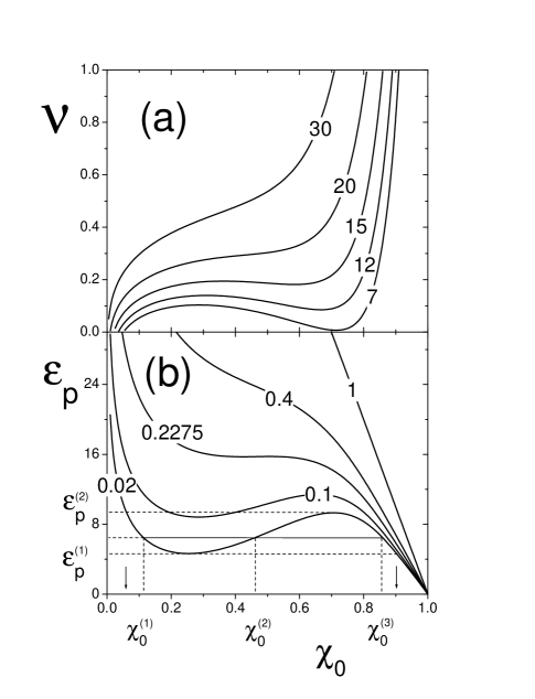
Figure 1: $\chi_{o}^{s}$ as a function of the control parameters $\nu$ (a) and $\varepsilon_{p}$ (b). The number on each curve is the value of $\varepsilon_{p}$ (a), $\nu$ (b).

The dependence of $\chi_{o}^{s}$ upon the control parameter $\varepsilon_{p}$ is shown in Fig. 1b for several values of $\nu$. Notice that, for example, the curve with $\nu=0.02$, for $\varepsilon_{p}^{(1)}<\varepsilon_{p}<\varepsilon_{p}^{(2)}$ has three possible values of $\chi_{0}^{s}$, that are labelled $\chi_{0}^{(1)}$, $\chi_{0}^{(2)}$, and $\chi_{0}^{(3)}$. We will show that two of them are stable and the other one is unstable. In addition, for $\nu_{c}\approx 0.2275$ we have the critical curve which separates curves which has regions of $\varepsilon_{p}$ with three possible solutions for $\chi_{0}^{s}$ from curves with just one solution. The critical point is given by $\varepsilon_{p}^{c}$, $\chi_{0}^{c}$ and $\nu_{c}$ that satisfy

$$\left(\frac{\partial\varepsilon_{p}}{\partial\chi_{o}}\right)_{\nu_{c}} = 0$$ (10)

$$\left(\frac{\partial^{2}\varepsilon_{p}}{\partial\chi_{o}^{2}}\right)_{\nu_{c}} = 0$$ (11)

We must point out that $\nu=\nu_{o}^{+}/ZN_{\mbox{\scriptsize max}}$, then Fig. 1b can be seen as a family of curves in which the electron-electron interaction is changed, for example, by changing the electron concentration. For GaAs bulk semiconductor, at 4 K, using $N=4.1\times 10^{17}$ cm^-3 and $T_{\mbox{\scriptsize e}}=300$ K in Eq. (8) we obtain $\nu=0.02$. The critical curve is obtained for $N=N_{c}\approx 6.11\times 10^{16}$ cm^-3.

The extrema of the curve $\varepsilon_{p}(\chi_{0}^{s})$ for a given $\nu$ are $\varepsilon_{p}^{(1)}$ and $\varepsilon_{p}^{(2)}$ respectively. They are found by solving the equation $(\partial\varepsilon_{p}/\partial\chi_{0})_{\nu}=0$. They are the boundaries of what is call the hysteresis region. If we increase $\varepsilon_{p}$ from a value less than $\varepsilon_{p}^{(1)}$, we will move until the maximum value $\varepsilon_{p}^{(2)}$ is reached. Then an abrupt jump will take place from a $\chi_{0}^{s}$ value at the maximum $\varepsilon_{p}^{(2)}$ to the value marked with the arrow at the left of Fig. 1b. As we decrease $\varepsilon_{p}$ from a value greater than $\varepsilon_{p}^{(2)}$ we will move until we reach the value of $\chi_{0}^{s}$ at the minimum. Then the system will undergo an abrupt jump to the value of $\chi_{0}^{s}$ marked with the right arrow in Fig. 1b. In Fig. 2 we show this hysteresis region for two values of the recombination parameter $\omega$.

Figure 2: Hysteresis region (hatched) in the phase space ($\nu$,$\varepsilon_{p}$) for two values of $\omega$.

Let us consider the perturbation to the steady state, $\chi(\varepsilon,\tau)=\chi^{s}(\varepsilon)+\delta\chi(\varepsilon,\tau)$ produced by a time dependent excitation, $\chi_{p}(t)=\chi_{p}^{s}+\delta\chi_{p}(t)$, where $\chi_{p}^{s}$ is the constant excitation that produces the steady state. Notice that $\chi_{\mbox{\scriptsize tot}}$ and $\chi_{0}$ are time dependent and they are given by the relations

$$\chi_{\mbox{\scriptsize tot}} = 1+\delta\chi_{\mbox{\scriptsize tot}}$$

$$\chi_{0} = \chi_{0}^{s}+\delta\chi_{0}$$ (12)

From Eq. (2) for $\chi_{0}$ and assuming that $\varepsilon_{p}>1$, we have for its steady state

$$\nu\chi_{1}^{s}+\chi_{1}^{s}-\chi_{0}^{s}+\chi_{0}^{s2}-\omega\chi_{0}^{s}=0$$ (13)

and the time evolution of its perturbation $\delta\chi_{0}$ is given by

$$\frac{d}{d\tau}\delta\chi_{0} = \nu\delta\chi_{1}+(\delta\chi_{1}-\delta\chi_{0})(1+\delta\chi_{\mbox{\scriptsize tot}})+\delta\chi_{\mbox{\scriptsize tot}}(\chi_{1}^{s}-\chi_{0}^{s})$$ (14)

$$+2\chi_{0}\delta\chi_{0}+(\delta\chi_{0})^{2}-\omega\delta\chi_{0}$$

which reduces to first order

$$\frac{d}{d\tau}\delta\chi_{0} = \nu\delta\chi_{1}+\delta\chi_{1}-\delta\chi_{0}+2\chi_{0}\delta\chi_{0}-\omega\delta\chi_{0}$$ (15)

$$= \left[\nu\frac{\delta\chi_{1}}{\delta\chi_{0}}+\frac{\delta\chi_{1}}{\delta\chi_{0}}-1+2\chi_{0}^{s}-\omega\right]\delta\chi_{0}$$

We now define the function $\psi(\chi_{0})$ that allows us to perform the stability analysis. From Eq. (13)

$$\psi(\chi_{0})\equiv\nu\chi_{1}+\chi_{1}-\chi_{0}+\chi_{0}^{2}-\omega\chi_{0}$$ (16)

and the steady state condition (Eq. (13)) becomes

$$\psi(\chi_{0}^{s})=0$$ (17)

The derivative of $\psi(\chi_{0})$ with respect of $\chi_{0}$ is

$$\frac{d\psi(\chi_{0})}{d\chi_{0}}=\nu\frac{d\chi_{1}}{d\chi_{0}}+\frac{d\chi_{1}}{d\chi_{0}}-1+2\chi_{0}-\omega$$ (18)

Now, in steady state $\chi_{1}^{s}$ is function of $\chi_{0}^{s}$ and the perturbation $\delta\chi_{1}$ is written as

$$\delta\chi_{1}=\left(\frac{d\chi_{1}}{d\chi_{0}}\right)_{\chi_{0}=\chi_{0}^{s}}\delta\chi_{0}$$

Therefore,

$$\frac{d}{d\tau}\delta\chi_{0}=\left.\frac{d\psi}{d\chi_{0}}\right|_{\chi_{0}=\chi_{0}^{s}}\delta\chi_{0}$$ (19)

and the solution for $\delta\chi_{0}$ is

$$\delta\chi_{0}(\tau)=\delta\chi_{0}(0)\exp\left[\left.\frac{d\psi}{d\chi_{0}}\right|_{\chi_{0}=\chi_{0}^{s}}\tau\right]$$ (20)

A steady state, given by a $\chi_{0}^{s}$, is stable if

$$\left.\frac{d\psi}{d\chi_{0}}\right|_{\chi_{0}=\chi_{0}^{s}}<0$$ (21)

Eq. (7) can be written as

$$-\frac{1}{\alpha}\ln\left[(1-\chi_{0}^{s})\chi_{0}^{s}\frac{\alpha}{\omega}\frac{\alpha+\beta}{e^{\alpha}-e^{-\beta}}\right]-\varepsilon_{p}=0$$ (22)

In steady state Eqs. (16) and (22) are equivalent, therefore

$$\psi(\chi_{0})=-\frac{1}{\alpha}\ln\left[(1-\chi_{0})\chi_{0}\frac{\alpha}{\omega}\frac{\alpha+\beta}{e^{\alpha}-e^{-\beta}}\right]-\varepsilon_{p}$$ (23)

In Fig. 1b we plotted $\varepsilon_{p}$ as a function of $\chi_{0}^{s}$ which means that we plotted the function $\psi(\chi_{0})$ and this establishes the stability of the states $\chi_{0}^{(1)}$, $\chi_{0}^{(2)}$, and $\chi_{0}^{(3)}$. The middle root is an unstable steady state, while $\chi_{0}^{(1)}$ and $\chi_{0}^{(3)}$ are stable steady states.

IV First order nonequilibrium phase transition and Maxwell construction

A thermodynamic system remains homogeneous and stable if the criteria of instrinsic stability is satisfiedstanley ,

$$\left(\frac{\partial P}{\partial V}\right)_{T}<0$$ (24)

where $P$ is the pressure of the system, $V$ is its volume and $T$ is its temperature. When this condition is violated a phase transition ocurrsstanley .

Then, from Eq. (21), we have the following correspondence note01

$$\chi_{0} \rightarrow V$$

$$\varepsilon_{p} \rightarrow P$$

$$\nu \rightarrow T$$

We see that Eq. ( 22) turns out to be the equation of state. The homogeneous states $\chi_{0}^{(1)}$ and $\chi_{0}^{(3)}$ are nonequilibrium stable steady states of the system. Therefore, we call the transition between states $\chi_{0}^{(1)}$ and $\chi_{0}^{(3)}$, a first order out of equilibrium phase transition. The order parameter is $\chi_{0}^{(3)}-\chi_{0}^{(1)}$ and still remains unknown.

So far, we have assumed that the populations $\chi_{0}$, $\chi_{1}$, and so on, are constants and homogeneous in space. Now, we assume that there exist spatial inhomogeneities, $\chi_{0}=\chi_{0}({\bf r})$, which produce spatial gradients, and diffusion of this population. We also assume, from the structure of Eq. (3), that the spatial and temporal behavior of the populations $\chi_{i}$, $i>0$, is given through $\chi_{0}$. Then, we have the following equation

$$\frac{\partial\chi_{0}}{\partial\tau}=\psi(\chi_{0})+\kappa\frac{\partial^{2}\chi_{0}}{\partial z^{2}}$$ (25)

We suppose, for simplicity, that $\chi_{0}$ depends only on the spatial coordinate $z$. Here, $\kappa$ is the $\chi_{0}$ difussion constant.

Let us introduce the “potential” $\Phi(\chi_{0})$ with the definitionpimpale ; schlogl

$$\psi(\chi_{0})=\frac{\partial}{\partial\chi_{0}}\Phi(\chi_{0})$$ (26)

Then, the steady state satisfies the equation

$$\kappa\frac{\partial^{2}\chi_{0}}{\partial z^{2}}=-\frac{\partial}{\partial\chi_{0}}\Phi(\chi_{0})$$ (27)

We have seen from Fig. 1b that, when $\nu=0.02$ and $\varepsilon_{p}$ is in the energy interval, $\varepsilon_{p}^{(1)}<\varepsilon_{p}<\varepsilon_{p}^{(2)}$, the system has two homogeneous stable steady states. Let us find a solution $\chi_{0}(z)$ such that, $\chi_{0}(+\infty)=\chi_{0}^{(1)}$ and $\chi_{0}(-\infty)=\chi_{0}^{(3)}$. In such a case two steady states coexist. Obviously, the “potential” $\Phi(\chi_{0})$ has two maxima in $\chi_{0}^{(1)}$ and $\chi_{0}^{(3)}$. Coexistence ocurrs for a value of $\varepsilon_{p}$ such that the two maxima are indistinguishable for the system,

$$\Phi(\chi_{0}^{(1)})=\Phi(\chi_{0}^{(3)})$$ (28)

Then

$$0 = \Phi(\chi_{0}^{(3)})-\Phi(\chi_{0}^{(1)})=\int_{\chi_{0}^{(1)}}^{\chi_{0}^{(3)}}d\chi_{0}\psi(\chi_{0})$$ (29)

$$= \int_{\chi_{0}^{(1)}}^{\chi_{0}^{(3)}}d\chi_{0}\;\left(\nu\chi_{1}+\chi_{1}-\chi_{0}+\chi_{0}^{2}-\omega\chi_{0}\right)$$

The last equation is the Maxwell construction for the vapor pressure in the van der Waals gas from which the order parameter $\chi_{0}^{(3)}-\chi_{0}^{(1)}$ can be calculated. We also notice that $-\Phi$ corresponds to the Hemholtz free potential. Moreover, the condition that $\Phi$ is at a maximum in a stable steady state corresponds to that the generalized free potential $H=-\Phi$ is at a minimum. This is consistent with the condition that an equilibrium thermodynamic system is in a state of minimum Hemholtz free energystanley .

V Conclusions

We have found carrier concentration bistabilities in a low temperature nonequilibrium electron gas and we study them in terms of the hysteresis region. The diffusion model consider here allows the coexistence of two phases of the open far from equilibrium gas. The phases are distinguished by the two values of carrier concentration at the bottom of the conduction band, namely, $\chi_{0}^{(1)}$ and $\chi_{0}^{(3)}$. These two corresponding homogeneous stable steady states are obtained using the Maxwell construction. We introduced the function $\psi$ and the stability condition for these states was given by Eq. (21). A generalized free potential was defined by Eq. (26) from which we obtained Eq. (29) that corresponds to the vapor pressure Maxwell construction of a van der Waals gas. The difference of the electron population in the bottom of the conduction band is the order parameter and is then calculated and goes to zero when $\nu$ approaches the critical value $\nu_{c}\approx 0.2275$. This is the reason we call this phase transition a first order nonequilibrium phase transition. For bulk GaAs at 4 K the critical curve is obtained using $N=N_{\mbox{\scriptsize c}}\approx 6.11\times 10^{16}$ cm^-3 and $T_{\mbox{\scriptsize e}}=300$ K in Eq. (8). We have to point out that the electron-electron interaction, which gives the nonlinear character of the rate equations, is the necessary main ingredient for the existence of the phase transition.

References

- (1) E. Schöll and H.G. Schuster (Editors), Handbook of Chaos Control, Second Edition. (John Wiley & Sons, New York, 2007); E. Schöll, Nonlinear Spatio-Temporal Dynamics and Chaos in Semiconductors. (Cambridge University Press, Cambridge, 2005).
- (2) E. Schöll, Nonequilibrium Phase Transitions in Semiconductors (Springer, Berlin, 1987); P. T. Landsberg, Eur. J. Phys. 1, 31 (1980); E. Schöll and P. T. Landsberg, Proc. R. Soc. Lond. A. 365, 495 (1979).
- (3) P. T. Landsberg and A. Pimpale, J. Phys. C: Solid State Phys. 9, 1243 (1976).
- (4) A. Pimpale and P. T. Landsberg, J. Phys. C: Solid State Phys. 10, 1447 (1977).
- (5) Hot Carriers in Semiconductors, Edited by M. Inoue, N. Sawaki, S. Tarucha, and C. Hamaguchi, Physica B 272 (1999); Hot Carriers in Semiconductors, Edited by K. Hess, J.-P. Leburton, and U. Ravaioli (Plenum Press, New York, 1996); Hot Carrier in Semiconductors, Edited by J. F. Ryan and A. C. Maciel, Semicon. Sc. Tech. 9 (1994); Hot Carrier in Semiconductors. Edited by J. Shah and G. J. Iafrate, Solid St. Electron. 31, Nos. 3/4 (1988); Hot Carrier in Semiconductors, Edited by D. G. Seiler and A. E. Stephens, Solid St. Electron. 21, No. 1 (1978).
- (6) The following papers present some results of the influence of the photoexcitation energy upon the electron gas effective temperature, photoluminiscence, and photoconductivity spectra. J. Shah, Solid St. Electron. 21, 43 (1978); E. Goebel and O. Hildebrand, Phys. Stat. Sol. (b) 88, 645 (1978); C. Weisbuch, Solid St. Electron. 21, 179 (1978); R. Ulbrich, Phys. Rev. Lett. 27, 1512 (1971).
- (7) J. L. Carrillo and J. Reyes, Phys. Rev. B29, 3172 (1984).
- (8) F. Schlögl, Z. Physik, 253, 147 (1972).
- (9) M.A. Rodríguez-Meza, Phys. Rev. B 64 233320 (2001).
- (10) J. L. Carrillo and M. A. Rodríguez, Phys. Rev. B44, 2934 (1991); M. A. Rodríguez-Meza, Doctoral Tesis, Universidad Autónoma de Puebla, México, unpublished (1988).
- (11) M.A. Rodríguez-Meza and J. L. Carrillo, Rev. Mex. Fis. 48, 52 (2002).
- (12) L. Meza-Montes, J. L. Carrillo, and M. A. Rodríguez, Physica B 225, 76 (1996); ibid 228, 279 (1996).
- (13) E.J. Yoffa, Phys. Rev. B23, 1909 (1981).
- (14) N. Takenaka, M. Inoue, and Y. Inuishi, J. Phys. Soc. Jpn. 47, 861 (1979).
- (15) J. Collet and T. Amand, J. Phys. Chem. Solids 47, 153 (1986); J. Collet, J.L. Oudar, and T. Amand, Phys. Rev. B34 5443 (1986).
- (16) H. Haug and A.-P. Jauho, Quantum Kinetics in Transport and Optics of Semiconductors, Springer Ser. Solid-State Sci., Vol. 123 (Springer-Verlag, Berlin Heidelberg, 1996).
- (17) J. Shah, Ultrafast Spectroscopy of Semiconductors and Semiconductor Nanostructures, 2nd edn. Springer Ser. Solid-State Sc. Vol. 115 (Springer-Verlag, Berlin Heidelberg, 1999).
- (18) P. A. Maksym, J. Phys. C: Solid State Phys. 15, 3127 (1982).
- (19) H. E. Stanley, Introduction to Phase Transitions and Critical Phenomena (Oxford University Press, New York, 1971).
- (20) A discussion on the corresponding thermodynamical variables is made in Ref. landsberg76 .