Nonparametric Estimation in Random Coefficients Binary Choice Models

Abstract.

This paper considers random coefficients binary choice models. The main goal is to estimate the density of the random coefficients nonparametrically. This is an ill-posed inverse problem characterized by an integral transform. A new density estimator for the random coefficients is developed, utilizing Fourier-Laplace series on spheres. This approach offers a clear insight on the identification problem. More importantly, it leads to a closed form estimator formula that yields a simple plug-in procedure requiring no numerical optimization. The new estimator, therefore, is easy to implement in empirical applications, while being flexible about the treatment of unobserved heterogeneity. Extensions including treatments of non-random coefficients and models with endogeneity are discussed.

1. Introduction

Consider a binary choice model

(1.1) $$Y=\mathbb{I}\left\{X^{\prime}\beta\geq 0\right\}$$

where $\mathbb{I}$ denotes the indicator function and $X$ is a $d$-vector of covariates. We assume that the first element of $X$ is 1, therefore the vector $X$ is of the form $X=(1,\tilde{X}^{\prime})^{\prime}$. The vector $\beta$ is random. The random element $(Y,\tilde{X},\beta)$ is defined on some probability space $(\Omega,\mathcal{F},\mathbb{P})$, and $(y_{i},\tilde{x}_{i},\beta_{i}),i=1,...,N$ denote its realizations. The econometrician observes $(y_{i},\tilde{x}_{i}),i=1,...,N$, but $\beta_{i},i=1,...,N$ remain unobserved. The vectors $\tilde{X}$ and $\beta$ correspond to observed and unobserved heterogeneity across agents, respectively. Note that the first element of $\beta$ in this formulation absorbs the usual scalar stochastic shock term as well as a constant in a standard binary choice model with non-random coefficients. This formulation is used in Ichimura and Thompson (1998), and is convenient for the subsequent development in this paper. Our basic model maintains exogeneity of the covariates $\tilde{X}$:

Assumption 1.1.

$\beta$ is independent of $\tilde{X}$,

Section 5.3 considers ways to relax this assumption. Under (1.1) and Assumption 1.1, the choice probability function is given by

$$r(x) =\mathbb{P}(Y=1|X=x)$$

$$=\mathbb{E}_{\beta}[\mathbb{I}\left\{x^{\prime}\beta>0\right\}].$$

Discrete choice models with random coefficients are useful in applied research since it is often crucial to incorporate unobserved heterogeneity in modeling the choice behavior of individuals. There is a vast and active literature on this topic. Recent contributions include Briesch, Chintagunta and Matzkin (1996), Brownstone and Train (1999), Chesher and Santos Silva (2002), Hess, Bolduc and Polak (2005), Harding and Hausman (2006), Athey and Imbens (2007), Bajari, Fox and Ryan (2007) and Train (2003). A common approach in estimating random coefficient discrete choice models is to impose parametric distributional assumptions. A leading example is the mixed Logit model, which is discussed in details by Train (2003). If one does not impose a parametric distributional assumption, the distribution of $\beta$ itself is the structural parameter of interest. The goal for the econometrician is then to recover it nonparametrically from the information about $r(x)$ obtained from the data.

Nonparametric treatments for unobserved heterogeneity distributions have been considered in the literature for other models. Heckman and Singer (1984) study the issue of unobserved heterogeneity distributions in duration models and propose a treatment by a nonparametric maximum likelihood estimator (NPMLE). Elbers and Ridder (1982) also develop some identification results in such models. Beran and Hall (1992) and Hoderlein et al. (2007) discuss nonparametric estimation of random coefficients linear regression models. Despite the tremendous importance of random coefficient discrete choice models, as exemplified in the above references, nonparametrics in these models is relatively underdeveloped. In their important paper, Ichimura and Thompson (1998) propose an NPMLE for the CDF of $\beta$. They present sufficient conditions for identification and prove the consistency of the NPMLE. The NPMLE requires high dimensional numerical maximization and can be computationally intensive even for a moderate sample size. Berry and Haile (2008) explore nonparametric identification problems in a random coefficients multinomial choice model that often arises in empirical IO.

This paper considers nonparametric estimation of the random coefficients distribution, using a novel approach that shares some similarities with standard deconvolution techniques. This allows us to reconsider the identifiability of the model and obtain a constructive identification result. Moreover, we develop a simple plug-in estimator for the density of $\beta$ that requires no numerical optimization or integration. It is easy to implement in empirical applications, while being flexible about the treatment of unobserved heterogeneity.

Since the scale of $\beta$ is not identified in the binary choice model, we normalize it so that $\beta$ is a vector of Euclidean norm 1 in ${\mathbb{R}}^{d}$. The vector $\beta$ then belongs to the $d-1$ dimensional sphere ${\mathbb{S}}^{d-1}$. This is not a restriction as long as the probability that $\beta$ is equal to 0 is 0. Also, since only the angle between $X$ and $\beta$ matters in the binary decision $\mathbb{I}\{X^{\prime}\beta\geq 0\}$, we can replace $X$ by $X/\|X\|$ without any loss of information. We therefore assume that $X$ is on the sphere ${\mathbb{S}}^{d-1}$ as well in the subsequent analysis. Results from the directional data literature are thus relevant to our analysis. We aim to recover the joint probability density function $f_{\beta}$ of $\beta$ with respect to the uniform spherical measure $\sigma$ over ${\mathbb{S}}^{d-1}$ from the random sample $(y_{1},x_{1}),\ldots,(y_{N},x_{N})$ of $(Y,X)$.

The problem considered here is a linear ill-posed inverse problem. We can write

(1.3) $$r(x)=\int_{b\in{\mathbb{S}}^{d-1}}\mathbb{I}\left\{x^{\prime}b\geq 0\right\}f_{\beta}(b)d\sigma(b)=\int_{H(x)}f_{\beta}(b)d\sigma(b):=\mathcal{H}\left(f_{\beta}\right)(x)$$

where the set $H(x)$ is the hemisphere $\left\{b:x^{\prime}b\geq 0\right\}$. The mapping $\mathcal{H}$ is called the hemispherical transformation. Inversion of this mapping was first studied by Funk (1916) and later by Rubin (1999). Groemer (1996) also discusses some of its properties. $\mathcal{H}$ is not injective without further restrictions and conditions need to be imposed to ensure identification of $f_{\beta}$ from $r$. Even under a set of assumptions that guarantee identification, however, the inverse of $\mathcal{H}$ is not a continuous mapping, making the problem ill-posed. To see this, suppose we restrict $f_{\beta}$ to be in ${{\rm L}^{2}}({\mathbb{S}}^{d-1})$. Since the kernel of $\mathcal{H}$ is square integrable by compactness of the sphere, it is Hilbert-Schmidt and thus compact. Therefore if the inverse of $\mathcal{H}$ were continuous, ${\mathcal{H}}^{-1}\mathcal{H}$ would map the closed unit ball in ${{\rm L}^{2}}({\mathbb{S}}^{d-1})$ to a compact set. But the Riesz theorem states that the unit ball is relatively compact if and only if the vector space has finite dimension. The fact that ${{\rm L}^{2}}({\mathbb{S}}^{d-1})$ is an infinite dimensional space contradicts this. Therefore the inverse of $\mathcal{H}$ cannot be continuous. In order to overcome this problem, we use a one parameter family of regularized inverses that are continuous and converge to the inverse when the parameter goes to infinity. This is a common approach to ill-posed inverse problems in statistics (see, e.g. Carrasco et al., 2007).

Due to the particular form of its kernel that involves the scalar product $x^{\prime}b$, the operator $\mathcal{H}$ is an analogue of convolution in ${\mathbb{R}}^{d}$, as illustrated in a simple example in Section A.1.1 of Supplemental Appendix. This analogy provides a clear insight into the identification issue. In particular, our problem is closely related to the so-called boxcar deconvolution (see, e.g. Groeneboom and Jongbloed (2003) and Johnstone and Raimondo (2004)), where identifiability is often a significant problem. The connection with deconvolution is also useful in deriving an estimator based on a series expansion on the Fourier basis on $\mathbb{S}^{1}$ or its extension to higher dimensional spheres called Fourier-Laplace series. These bases are defined via the Laplacian on the sphere, and they diagonalize the operator $\mathcal{H}$ on ${{\rm L}^{2}}\left({\mathbb{S}}^{d-1}\right)$. Such techniques are used in Healy and Kim (1996) for nonparametric empirical Bayes estimation in the case of the sphere $\mathbb{S}^{2}$. The kernel of the integral operator $\mathcal{H}$, however, does not satisfy the assumptions made by Healy and Kim. Unlike Healy and Kim (1996), we make use of so-called “condensed” harmonic expansions. The approach replaces a full expansion on a Fourier-Laplace basis by an expansion in terms of the projections on the finite dimensional eigenspaces of the Laplacian on the sphere. This is useful since an explicit expression of the kernel of the projector is available. It enables us to work in any dimension and does not require a parametrization by hyperspherical coordinates nor the actual knowledge of an orthonormal basis. This approach, to the best of our knowledge, appears to be new in the econometrics literature.

The paper is organized as follows. Section 2 provides a practical guide for our procedure, which is easy to implement. Section 3 deals with identification while introducing basic notions used throughout the paper. We derive the convergence rates of the estimators in all the ${\rm L}^{q}$ spaces for $q\in[1,\infty]$ and also prove a pointwise CLT in Section 4. Some extensions, such as estimation of marginals, treatments of models with non-random coefficients, and the case with endogenous regressors are presented in Section 5. Simulation results are reported in Section 6. Section 7 concludes. Supplemental Appendix presents analysis of a toy model, technical tools used in the main text, estimators for choice probabilities that are used to construct our density estimators, and the proofs of the main results.

2. A Brief Guide for Practical Implementation

This section presents our basic estimation procedure when a random sample $\{(y_{i},\tilde{x}_{i})\}$ generated from the model (1.1) is available. As noted in Section 1, normalize covariates data and define $x_{i}=(1,\tilde{x}_{i}^{\prime})/\|(1,\tilde{x}_{i}^{\prime})\|\in\mathbb{S}^{d-1},i=1,...,N$. To estimate the joint density of the random vector $\beta$, use the following formula:

(2.1) $$\hat{f}_{\beta}(b)=\max\left(\frac{2}{|\mathbb{S}^{d-1}|}\sum_{p=0}^{T_{N}-1}\frac{\chi(2p+1,2T_{N})h(2p+1,d)}{\lambda(2p+1,d)C_{2p+1}^{\nu(d)}(1)}\left(\frac{1}{N}\sum_{i=1}^{N}\frac{(2y_{i}-1)C_{2p+1}^{\nu(d)}(x_{i}^{\prime}b)}{\max\left(\hat{f}_{X}(x_{i}),m_{N}\right)}\right),0\right).$$

The factors $|{\mathbb{S}}^{d-1}|$, $\chi$, $h$ and $\lambda$ are constants that do not depend on data and trivial to compute. The surface area $\left|{\mathbb{S}}^{d-1}\right|$ of ${\mathbb{S}}^{d-1}$ is given by $\left|{\mathbb{S}}^{d-1}\right|=\frac{2\pi^{d/2}}{\Gamma(d/2)}$ where $\Gamma$ denotes the Gamma function. The constants $h$, $\nu$ and $\lambda$ are obtained via the numerical formulas $h(n,d)=\frac{(2n+d-2)(n+d-2)!}{n!(d-2)!(n+d-2)}$, $\nu(d)=(d-2)/2$ and $\lambda(2p+1,d)=\frac{(-1)^{p}|\mathbb{S}^{d-2}|1\cdot 3\cdots(2p-1)}{(d-1)(d+1)\cdots(d+2p-1)}$, respectively. The function $\chi$ is defined on $\mathbb{N}\times\mathbb{N}$ and used for smoothing. This is to be chosen by the user: see Proposition A.3 as well as the numerical example reported in Section 6 for examples of $\chi$. The truncation parameter $T_{N}$ needs to be chosen so that it grows with the sample size with a sufficiently slow rate. The trimming factor $m_{N}$ is also user-defined, and it is chosen so that it goes to zero as the sample size increases. The notation $C_{n}^{\nu}(\cdot)$ signifies the Gegenbauer polynomial; They, for example, correspond to the Chebychev polynomials of the first kind in the case of one random slope (i.e. the case with $d=2$). The only remaining factor which needs to be calculated in the above formula is the nonparametric density estimator $\hat{f}_{X}$ for $f_{X}$ on ${\mathbb{S}}^{d-1}$. For example, the following nonparametric estimator can be used:

(2.2) $$\hat{f}_{X}(x)=\max\left(\frac{1}{|\mathbb{S}^{d-1}|}\sum_{n=0}^{T_{N}^{\prime}}\frac{\chi(n,T_{N}^{\prime})h(n,d)}{C_{n}^{\nu(d)}(1)}\left(\frac{1}{N}\sum_{i=1}^{N}C_{n}^{\nu(d)}(x_{i}^{\prime}x)\right),0\right)$$

where $T_{N}^{\prime}$ is an another truncation parameter, playing a role similar to $T_{N}$.

Our estimator $\hat{f}_{\beta}$ requires neither numerical integration nor optimization. This is a clear advantage over existing estimators for random coefficient binary choice models, including many parametric estimators. This is our main proposal, on which the rest of the paper focuses. In Section 4 we explain how the formula (2.1) is derived, and investigate its asymptotic properties.

3. Identification Analysis

In this section we address the following two questions:

1. Under what conditions is $f_{\beta}$ identified?

2. Does the random coefficients model impose restrictions?

To answer these questions it is useful to introduce the notion of the odd and even part of a function defined on the sphere.

Definition 3.1.

We denote the odd part and the even part of a function $f$ by

$$f^{-}(b)=(f(b)-f(-b))/2$$

and

$$f^{+}(b)=(f(b)+f(-b))/2,$$

respectively, for every $b$ in ${\mathbb{S}}^{d-1}$.

Let us start with the question (Q1). As noted in Section A.1.4, operating $\mathcal{H}$ reduces the even part of a function to a constant 1 and therefore it is impossible to recover $f_{\beta}^{+}$ from the knowledge of $r$, which is what observations offer. Our identification strategy is therefore as follows: (Step 1) Assume conditions that guarantee the identification of $f_{\beta}^{-}$; then (Step 2) Show that $f_{\beta}$ is uniquely determined from $f_{\beta}^{-}$ under a reasonable assumption. We first consider Step 1. Define $H^{+}=H({\bf n})=\{x\in{\mathbb{S}}^{d-1}:\ x^{\prime}{\bf n}\geq 0\}$, where ${\bf n}=(1,,0,...,0)^{\prime}$, that is, the northern hemisphere of $\mathbb{S}^{d-1}$. For later use, also define its southern hemisphere $H^{-}=H(-\bf n)$. Since the model we consider has a constant as the first element of the covariate vector before normalization, the same vector after normalization is necessarily an element of $H^{+}$. We make the following assumption, which also appears in Ichimura and Thompson (1998), and show that it achieves Step 1.

Assumption 3.1.

The support of $X$ is $H^{+}$.

This assumption demands that $\tilde{X}$, the vector of non-constant covariates in the original scale, is supported on the whole space ${\mathbb{R}}^{d-1}$. It rules out discrete or bounded covariates; see Section 5 for a potential approach to deal with regressors with limited support. In what follows we assume that the law of $X$ is absolutely continuous with respect to $\sigma$ and denote its density by $f_{X}$. Step 1 of our identification argument is to show that the knowledge of $r(x)$ on $H^{+}$, which is available under Assumption 3.1, identifies $f_{\beta}^{-}$. The problem at hand calls for solving $r=\mathcal{H}f_{\beta}=\frac{1}{2}+\mathcal{H}f_{\beta}^{-}$ for $f_{\beta}^{-}$, and the inversion formula derived in (4.1) is potentially useful for the purpose. A direct application of the formula to $r$ is inappropriate, however, since it requires integration of $r$ on the whole sphere $\mathbb{S}^{d-1}$, but $r$ is defined only on $H^{+}$ even when $\tilde{X}$ has full support on $\mathbb{R}^{d-1}$. An appropriate extension of $r(x),x\in H^{+}$ to the entire $\mathbb{S}^{d-1}$ is in order. Using the random coefficients model (1.1) and Assumption 1.1, then noting that $f_{\beta}$ is a probability density function, conclude

(3.1) $$\mathcal{H}(f_{\beta})(-x)=\int_{H(-x)}f_{\beta}(b)d\sigma(b)=1-\mathcal{H}(f_{\beta})(x)=1-r(x)$$

for $x$ in $H^{+}$. This suggests an extension $R$ of $r$ to $\mathbb{S}^{d-1}$ as follows:

(3.2) $$\forall x\in H^{+},R(x)=r(x),\ {\rm and}\ \forall x\in H^{-},R(x)=1-r(-x)=1-R(-x).$$

The function $R$ is well-defined on the whole sphere under Assumption 3.1. Later we derive a formula for $f_{\beta}^{-}$ in terms of $R(x),x\in\mathbb{S}^{d-1}$, which shows the identifiability of $f_{\beta}^{-}$ under Assumption 3.1.

Note that

(3.3) $$R(x) =R^{+}(x)+R^{-}(x)$$

$$=\frac{1}{2}\left[R(x)+R(-x)\right]+R^{-}(x)$$

$$=\frac{1}{2}\left[R(x)+(1-R(x))\right]+R^{-}(x)\quad\text{ by (\ref{e2bb})}$$

$$=\frac{1}{2}+R^{-}(x)$$

thus $R$ is completely determined by its odd part and therefore,

$$R(x)=\frac{1}{2}+\mathcal{H}\left(f_{\beta}^{-}\right)(x),$$

or

(3.4) $$R^{-}=\mathcal{H}f_{\beta}^{-}.$$

We can invert this equation to obtain $f_{\beta}^{-}$.

Now we turn to Step 2 in our identification argument. Obviously $f_{\beta}^{-}$ does not uniquely determine $f_{\beta}$ without further assumptions. This is a fundamental identification problem in our model. We need to identify $f_{\beta}$ from the choice probability function $r$, but we can choose an appropriate even function $g$ so that $f_{\beta}+g$ is a legitimate density function (see the proof of Proposition 3.1 for such a construction). Then $r=\mathcal{H}\left(f_{\beta}+g\right)$, and the knowledge of $r$ identifies $f_{\beta}$ only up to such a function $g$. Ichimura and Thompson (1998, Theorem 1) give a set of conditions that imply the identification of the model (1.1). One of their assumptions postulates that there exists $c$ on ${\mathbb{S}}^{d-1}$ such that ${\mathbb{P}}(c^{\prime}\beta>0)=1$. This, in our terminology, means that:

Assumption 3.2.

The support of $\beta$ is a subset of some hemisphere.

As noted by Ichimura and Thompson (1998), Assumption 3.2 does not seem too stringent in many economic applications. It is often reasonable to assume that an element of the random coefficients vector, such as a price coefficient, has a known sign. If the $j$-th element of $\beta$ has a known sign (and positive), then Assumption 3.2 holds with $c$ being a unit vector with its $j$-th element being 1. This is a case in which the location of the hemisphere in Assumption 3.2 is known a priori, though the knowledge about its location is not necessary for identification. Assumption 3.2 implies the following mapping from $f_{\beta}^{-}$ to $f_{\beta}$ developed in (A.24):

(3.5) $$f_{\beta}(b)=2f_{\beta}^{-}(b)\mathbb{I}\left\{f_{\beta}^{-}(b)>0\right\}.$$

This is useful because it shows that Assumption 3.2 guarantees identification if $f_{\beta}^{-}$ is identified. Moreover, it will be used in the next section to develop a key formula that leads to a simple and practical estimator for $f_{\beta}$ that is guaranteed to be non-negative.

Remark 3.1.

Assumption 3.2 is testable since it imposes restrictions on $f_{\beta}^{-}$, which is identified under weak conditions. For example, for values of $b$ with $f_{\beta}^{-}(b)>0$, $f_{\beta}^{-}(-b)<0$ must hold. Or, it implies that $f_{\beta}^{-}$ integrates to $1/(2|{\mathbb{S}}^{d-1}|)$ on a hemisphere $H(x)$ for some $x$, and $-1/(2|{\mathbb{S}}^{d-1}|)$ on the other $H(-x)$.

The subsequent result, Proposition 3.1, answers question (Q2), and a proof is given in Supplemental Appendix.

Notation.

We use the notation ${{\rm L}^{2}}({\mathbb{S}}^{d-1})$ for the space of square integrable complex valued functions equipped with the hermitian product $(f,g)_{{{\rm L}^{2}}({\mathbb{S}}^{d-1})}=\int_{{\mathbb{S}}^{d-1}}f(x)\overline{g}(x)d\sigma(x)$, and more generally use ${\rm L}^{p}({\mathbb{S}}^{d-1})$ for $p\in[1,\infty]$ the Banach space of $p$-integrable functions and $\|\cdot\|_{p}$ the corresponding norm. We also use the notation ${\rm W}^{s}_{p}({\mathbb{S}}^{d-1})$ (and ${\rm H}^{s}({\mathbb{S}}^{d-1})$ for $p=2$) to signify the corresponding Sobolev spaces with norm $\|\cdot\|_{p,s}$ defined as

$$\|f\|_{p,s}=\|f\|_{p}+\left\|\left(-\Delta^{S}\right)^{s/2}f\right\|_{p}$$

where $\Delta^{S}$ denotes the Laplacian on the Sphere $\mathbb{S}^{d-1}$: See Section A.1.3 for further discussions.

Proposition 3.1.

A $[0,1]$-valued function $r$ is compatible with the random coefficients model (1.1) with $f_{\beta}$ in ${{\rm L}^{2}}({\mathbb{S}}^{d-1})$ and Assumption 1.1 if and only if $r$ is homogeneous of degree 0 and its extension $R$ according to (3.2) belongs to ${\rm H}^{d/2}({\mathbb{S}}^{d-1})$.

The global smoothness assumption that $R$ belongs to ${\rm H}^{d/2}({\mathbb{S}}^{d-1})$ imposes substantial restriction on the property of observables, that is, the behavior of the choice probability function $r$. Note that the smoothness condition in this proposition is stated in terms of $R$, and even if the choice probability function $r$ is sufficiently smooth on the support of $X$, which is $H^{+}$, it is not necessarily consistent with the random coefficients binary choice model (1.1) unless its extension is smooth globally on $\mathbb{S}^{d-1}$. In particular, the Sobolev embedding of ${\rm H}^{s}({\mathbb{S}}^{d-1})$ into the space of continuous functions for $s>(d-1)/2$ implies that if the extension $R$ is in ${\rm H}^{d/2}({\mathbb{S}}^{d-1})$, it has to be continuous on $\mathbb{S}^{d-1}$. This, in turn, means that the corresponding $r$ has to satisfy certain matching conditions at a boundary point $x$ of $H^{+}$ (i.e. $x^{\prime}\mathbf{n}=0$) and its opposite point $-x$.

4. Nonparametric Estimation of $f_{\beta}$

4.1. Derivation of the closed form estimation formula

This section discusses how the closed form estimation formula (2.1) is derived. Suppose an odd function $f^{-}$ defined on $\mathbb{S}^{d-1}$ satisfies an integral equation $f^{-}=Hg$ with $g$ square integrable with respect to the spherical measure. In Section A.1.4 we show that the solution to this equation is given by:

(4.1) $$\mathcal{H}^{-1}(f^{-})(y)=\sum_{p=0}^{\infty}\frac{1}{\lambda(2p+1,d)}\int_{\mathbb{S}^{d-1}}q_{2p+1,d}(x,y)f^{-}(x)d\sigma(x)$$

where expressions for $\lambda$ and $q$ are provided in Proposition A.4 and Theorem A.1, respectively. If an appropriate estimator $\hat{R}^{-}$ of $R^{-}$ is available, an application of the inversion formula (4.1) to (3.4) suggests the following estimator for $f_{\beta}^{-}$:

(4.2) $$\hat{f}_{\beta}^{-} =\mathcal{H}^{-1}\left(\hat{R}^{-}\right)$$

$$=\sum_{p=0}^{\infty}\frac{1}{\lambda(2p+1,d)}\int_{{\mathbb{S}}^{d-1}}q_{2p+1,d}(\cdot,x)\hat{R}^{-}(x)d\sigma(x).$$

Then use the mapping (3.5) to define

(4.3) $$\hat{f}_{\beta}(b)=2\hat{f}_{\beta}^{-}(b)\mathbb{I}\left\{\hat{f}_{\beta}^{-}(b)>0\right\}$$

as an estimator for $f_{\beta}$.

We use the following notation in the rest of the paper:

Notation.

For two sequences of positive numbers $(a_{n})_{n\in{\mathbb{N}}}$ and $(b_{n})_{n\in{\mathbb{N}}}$, we write $a_{n}\asymp b_{n}$ when there exists a positive $M$ such that $M^{-1}b_{n}\leq a_{n}\leq Mb_{n}$ for every positive $n$.

Proposition A.6 implies that if $\hat{f}_{\beta}^{-}-f_{\beta}^{-}\in{\rm H}^{s}({\mathbb{S}}^{d-1})$ then $\hat{R}^{-}-R^{-}\in{\rm H}^{\sigma}({\mathbb{S}}^{d-1})$, $\sigma=s+\frac{d}{2}$ and for $v\in[0,s]$,

(4.4) $$\|\hat{f}_{\beta}^{-}-f_{\beta}^{-}\|_{2,v}\asymp\|\hat{R}^{-}-R^{-}\|_{2,v+d/2}.$$

As discussed earlier, the estimation of $f_{\beta}$ is related to deconvolution in $\mathbb{S}^{d-1}$, and the degree of ill-posedness in our model is $d/2$, which is indeed the rate at which the absolute values of the eigenvalues of $\mathcal{H}$ (c.f. Proposition A.4) $\lambda(n,d),n=2p+1,p\in\mathbb{N}$ converges to zero as $p$ grows, as shown in (A.27). Existing results for deconvolution problems (see, for example, Fan, 1991 and Kim and Koo, 2000) then suggest that we should be able to estimate $f_{\beta}$ at the rate $N^{-\frac{s}{2s+2d-1}}$ in the L${}^{2}(\mathbb{S}^{d-1})$ provided that $f_{\beta}\in{\rm H}^{s}({\mathbb{S}}^{d-1})$. The relationship (4.4), evaluated at $v=0$, implies that this can be achieved if we can estimate $R^{-}$ at the rate $N^{-\frac{\sigma-\frac{d}{2}}{2\sigma+d-1}}$ in the $\|\cdot\|_{2,d/2}$ norm. The latter is the usual nonparametric rate for estimation of densities on $d-1$ dimensional smooth submanifolds of $\mathbb{R}^{d}$ (see, for example, Hendriks, 1990).

The estimation formula given in (4.2) is natural and reasonable, though it typically requires numerical evaluation of integrals to implement it. Moreover, in practice one needs to evaluate the infinite sum in (4.2), for example, by truncating the series. This results in a general estimator that can be written in the following two equivalent forms

(4.5) $$\hat{f}_{\beta}^{-} =\mathcal{H}^{-1}\left(P_{\tilde{T}_{N}}\hat{R}^{-}\right)$$

$$=\sum_{p=0}^{T_{N}}\frac{1}{\lambda(2p+1,d)}\int_{{\mathbb{S}}^{d-1}}q_{2p+1,d}(\cdot,x)\hat{R}^{-}(x)d\sigma(x)$$

for suitably chosen $\tilde{T}_{N}$ that goes to infinity with $N$ and $P_{\tilde{T}_{N}}$ defined in (A.20). The sequence $\mathcal{H}^{-1}\circ P_{\tilde{T}_{N}},N=1,2,...$ can be interpreted as regularized inverses of $\mathcal{H}$, with the spectral cut-off method often used in statistical inverse problems.

We now discuss how to obtain $\hat{R}^{-}$ in the calculation of (4.5). The following choice is particularly convenient:

(4.6) $$\hat{R}^{-}(x)=\frac{1}{N}\sum_{i=1}^{N}\frac{(2y_{i}-1)K_{2T_{N}}^{-}(x_{i},x)}{\max\left(\hat{f}_{X}(x_{i}),m_{N}\right)}$$

where $m_{N}$ is a trimming factor going to 0 with the sample size, $K^{-}(x_{i},\cdot)$ denotes the odd part (of the second argument) of the kernel function $K(x_{i},\cdot)$ defined in (A.23) and $\hat{f}_{X}$ is a nonparametric density estimator for $f_{X}$. See Section A.1.5 of Supplemental Appendix for the derivation of the above formula. Various nonparametric estimators for $f_{X}$ can be used in (4.6), since estimation of densities on compact manifolds have been studied by several authors, using histogram (Ruymgaart (1989)), projection estimators (see, e.g. Devroye and Gyorfi (1985) for the circle and Hendriks (1990) for general compact Riemannian manifolds) or kernel estimators (see, e.g. Devroye and Gyorfi (1985) for the case of the circle, and Hall et al. (1987) and Klemelä (2000) for higher dimensional spheres). Note also that Baldi et al. (2009) develops an adaptive density estimator on the sphere using needlet thresholding. In the simulation experiment we use

(4.7) $$\hat{f}_{X}(x)=\max\left(\frac{1}{N}\sum_{i=1}^{N}K_{T_{N}^{\prime}}(x_{i},x),0\right)$$

for a suitably chosen $T_{N}^{\prime}$ that depends on the sample size and the smoothness of $f_{X}$ and $K_{T_{N}^{\prime}}$ is a kernel of the form (A.23) satisfying Assumption A.1. Note that its rate of convergence in sup-norm can be obtained in the same manner as the proof of Theorem 4.1. This estimator is in the spirit of the projection estimators of Hendriks (1990), but here we are able to derive a closed form using the condensed harmonic expansions together with the Addition Formula. Note also that $K_{T_{N}}$ is a smoothed projection kernel (note the factor $\chi$ in (A.23)), which is used here in order to have good approximation properties in the ${\rm L}^{q}({\mathbb{S}}^{d-1})$ norms with arbitrary $q\in[1,\infty]$, in particular in the ${\rm L}^{\infty}({\mathbb{S}}^{d-1})$ norm.

Using (4.5) and (4.6) with $\tilde{T}_{N}=2T_{N}$, define

$$\hat{f}_{\beta}^{-}=\mathcal{H}^{-1}\left(\hat{R}^{-}\right)=\mathcal{H}^{-1}\left(\frac{1}{N}\sum_{i=1}^{N}\frac{(2y_{i}-1)K_{2T_{N}}^{-}(x_{i},\cdot)}{\max\left(\hat{f}_{X}(x_{i}),m_{N}\right)}\right).$$

Computing $\hat{f}^{-}_{\beta}$ is straightforward. First, note that the estimator (4.6) for $R^{-}$ resides in a finite dimensional space $\bigoplus_{p=0}^{T_{N}}H^{2p+1,d}$, therefore $P_{2T_{N}}\hat{R}^{-}=\hat{R}^{-}$ holds. Consequently, unlike in (4.5) where a general estimator for $R^{-}$ is considered, we do not need to apply any additional series truncation to $\hat{R}^{-}$ prior to the inversion of $\mathcal{H}$. Second, the estimator requires no numerical integration. To see this, note the formula

$$\mathcal{H}^{-1}\left(K_{2T_{N}}^{-}(x_{i},\cdot)\right)(b)=\sum_{p=0}^{T_{N}-1}\frac{\chi(2p+1,2T_{N})}{\lambda(2p+1,d)}q_{2p+1,d}(x_{i},b),$$

which follows from

$$\int_{\mathbb{S}^{d-1}}q_{2p+1,d}(x,b)K_{2T_{N}}^{-}(x,x_{i})d\sigma(x) =\int_{\mathbb{S}^{d-1}}q_{2p+1}(x,b)\sum_{p^{\prime}=1}^{T_{N}-1}\chi(2p^{\prime}+1,2T_{N})q_{2p^{\prime}+1,d}(x,x_{i})d\sigma(x)$$

$$=\chi(2p+1,2T_{N})q_{2p+1,d}(b,x_{i}).$$

which, in turn, can be seen by the definition of $K_{T}$ in (A.23), the fact that the integral operators with $q$ as kernels are projections and (A.16). Thus

$$\hat{f}_{\beta}^{-}(b)=\frac{1}{N}\sum_{i=1}^{N}\frac{2y_{i}-1}{\max\left(\hat{f}_{X}(x_{i}),m_{N}\right)}\sum_{p=0}^{T_{N}-1}\frac{\chi(2p+1,2T_{N})}{\lambda(2p+1,d)}q_{2p+1,d}(x_{i},b).$$

Using (4.3) and the Addition formula (Theorem A.1), we arrive at an estimator for $f_{\beta}$ with the following explicit form:

(4.8) $$\hat{f}_{\beta}(b)=2\hat{f}_{\beta}^{-}(b)\mathbb{I}\{\hat{f}_{\beta}^{-}(b)>0\},$$

where $$\hat{f}_{\beta}^{-}(b)=\frac{1}{|\mathbb{S}^{d-1}|}\sum_{p=0}^{T_{N}-1}\frac{\chi(2p+1,2T_{N})h(2p+1,d)}{\lambda(2p+1,d)C_{2p+1}^{\nu(d)}(1)}\left(\frac{1}{N}\sum_{i=1}^{N}\frac{(2y_{i}-1)C_{2p+1}^{\nu(d)}(x_{i}^{\prime}b)}{\max\left(\hat{f}_{X}(x_{i}),m_{N}\right)}\right).$$

This is equivalent to the formula (2.1) previously presented in Section 2. Likewise, using the definition of the smoothing kernel (A.23) and the Addition Theorem in the above definition (4.7) of $\hat{f}_{X}$, we obtain the formula (2.2) as well.

4.2. Rates of Convergence in ${\rm L}^{q}({\mathbb{S}}^{d-1})$-norms

Now we analyze the rate of our estimator $\hat{f}_{\beta}$. The following assumption is weak and reasonable.

Assumption 4.1.

$f_{X}\in{\rm L}^{\infty}$.

The proofs of the following theorems and corollaries in the rest of this section are given in Section A.1.6 of Supplemental Appendix.

Theorem 4.1 (Upper bounds in ${\rm L}^{q}({\mathbb{S}}^{d-1})$).

Suppose Assumptions A.1, 3.1 and 4.1 hold, and choose $T_{N}$ that does not grow more than polynomially fast in $N$. If $f_{\beta}^{-}$ belongs to ${\rm W}_{q}^{s}({\mathbb{S}}^{d-1})$ with $q$ in $[1,\infty]$ and $s>0$, and

(4.9) $$\max_{i=1,\ldots,N}\left|f_{X}(x_{i})-\hat{f}_{X}(x_{i})\right|=O_{p}\left(m_{N}\right),$$

then, for any $1\leq r\leq q$,

$$\left\|\hat{f}_{\beta}-f_{\beta}\right\|_{q}=O_{p} \left(m_{N}^{-1}N^{-1/2}T_{N}^{(2d-1)/2}(\log N)^{(1/2-1/q)\mathbb{I}\{q\geq 2\}}\right.$$

$$\ +T_{N}^{-s}+T_{N}^{d/2}m_{N}^{-2}\max_{i=1,\ldots,N}\left|f_{X}(x_{i})-\hat{f}_{X}(x_{i})\right|$$

(4.10) $$\ \left.T_{n}^{d/2+(d-1)(1-1/r)}\sigma\left(f_{X}<m_{N}\right)^{1/q-1/r+1}\right).$$

When there exists $m>0$ such that $f_{X}\geq m\ \sigma\ a.e.$ on $H^{+}$, the following holds for the estimator without the trimming factor (i.e. $m_{N}$ = 0) when the estimator $\hat{f}_{X}$ which is consistent in sup norm:

$$\left\|\hat{f}_{\beta}-f_{\beta}\right\|_{q}=O_{p} \left(N^{-1/2}T_{N}^{(2d-1)/2}(\log N)^{(1/2-1/q)\mathbb{I}\{q\geq 2\}}\right.$$

$$\ \left.+T_{N}^{-s}+T_{N}^{d/2}\max_{i=1,\ldots,N}\left|f_{X}(x_{i})-\hat{f}_{X}(x_{i})\right|\right).$$

The first term in (4.10) is the stochastic error, the second term is the approximation bias, the third the plug-in error and the fourth the trimming bias. Note that Theorem 4.1 imposes the mild assumption (4.9); otherwise, we need to replace $T_{N}^{d/2}m_{N}^{-2}\max_{i=1,\ldots,N}\left|f_{X}(x_{i})-\hat{f}_{X}(x_{i})\right|$ in (4.10) with $T_{N}^{d/2}m_{N}^{-2}\max_{i=1,\ldots,N}\left|f_{X}(x_{i})-\hat{f}_{X}(x_{i})\right|\left(1+(\log N)^{(1/2-1/q)\mathbb{I}\{q\geq 2\}}N^{-1/2}T_{N}^{(d-1)/2}\right)$. Since

$$\max_{i=1,\ldots,N}\left|f_{X}(x_{i})-\hat{f}_{X}(x_{i})\right|\leq\left|f_{X}-\hat{f}_{X}\right|_{\infty},$$

this term can be made of order $O_{P}\left(\left(\frac{N}{\log N}\right)^{-v/(2v+d-1)}\right)$ when $f_{X}\in{\rm W}_{\infty}^{v}$ with a suitably chosen parameter $T_{N}^{\prime}$ if we take (4.7) as an estimator. The proof of the latter statement is classical and can be obtained simplifying the proof of Theorem 4.1 and Corollary 4.1. Equation (4.10) yields that, for proper choices of $m_{N}$ going to zero and $T_{N}$ to infinity, $\hat{f}_{\beta}$ is consistent given that $f_{X}$ has some smoothness in the Sobolev scales.

Though the additional condition of $f_{X}$ being bounded away from 0 in the last statement of Theorem 4.1 is convenient, it is restrictive. To see this, consider the $d=2$ case. In polar coordinates, $f_{X}\left(\cos(\theta),\sin(\theta)\right)=f_{\tilde{X}}(\tan(\theta))(1+\tan^{2}(\theta)$, thus, assuming $f_{X}\geq m$ on $H^{+}$, which does not require trimming, yields

$$\forall x\in{\mathbb{R}},f_{\tilde{X}}(x)\geq\frac{m}{1+x^{2}}.$$

It implies that $\tilde{X}$ has tails larger than Cauchy tails and all moments are infinite. The introduction of the trimming factor $m_{N}$ allows us to relax the assumption $f_{X}\geq m$, though it introduces bias. As is clear from (4.10), the condition for the trimming bias to go to zero with $N$ depends both on $T_{N}$ and $m_{N}$. The quantity $\sigma(f_{X}<m_{N})$ should decay to zero with $N$ sufficiently fast. We can check, for example, that when $\tilde{X}$ is standard Gaussian then $\sigma(f_{X}<m_{N})=O\left((-\log m_{N})^{-1/2}\right)$, when it is Laplace then $\sigma(f_{X}<m_{N})=O\left((-\log m_{N})^{-1}\right)$ and when $f_{\tilde{X}}$ is proportional to $(1+x^{2})^{-k}$ with $k>1$ we obtain that $\sigma(f_{X}<m_{N})=O\left(m_{N}^{1/(2(k-1))}\right)$. In all these cases, it is possible to adjust adequately $T_{N}$ and $m_{N}$ and to obtain rates of convergence. The upper bound on the rates become slower as the tail of $f_{X}$ becomes thinner.

Nonparametric estimation of the regression function with random degenerate design, in the sense that the density of regressors can be low on its support, is a difficult issue. It has been studied for the pointwise risk in Hall et al. 1997, Gaïffas 2005, Gaïffas 2009 and Guerre 1999. Extension to inverse problems setting is a widely open problem. We tackle this problem for our specific inverse problem. Future research includes the study of lower bounds from the minimax point of view that account for the degeneracy of the design.

Let us now return to the general case of $d-1$ regressors. The assumptions below allow us to obtain rates that differ slightly from the rates that we would obtain in the ideal case where $f_{X}\geq m\ \sigma\ a.e.$ for positive $m$ on $H^{+}$.

Assumption 4.2.

Suppose for $q$ in $[1,\infty]$, there exist positive $\tau$ and $r_{X}$ such that

1. $\sigma(f_{X}<h)=O(h^{\tau})$ and $f_{X}\in{\rm L}^{\infty},$
   and either

2. $$\max_{i=1,\ldots,N}\left|f_{X}(x_{i})-\hat{f}_{X}(x_{i})\right|=O_{p}\left(\left(\frac{N}{(\log N)^{(1-2/q)\mathbb{I}\{q\geq 2\}}}\right)^{-r_{X}}\right)$$

   
   

   or,

3. for some constant $C$,

   $$\overline{\lim}_{N\rightarrow\infty}\left(\frac{N}{(\log N)^{(1-2/q)\mathbb{I}\{q\geq 2\}}}\right)^{r_{X}}\max_{i=1,\ldots,N}\left|f_{X}(x_{i})-\hat{f}_{X}(x_{i})\right|\leq C\quad a.s.$$

   
   

   holds.

As seen before, Assumption 4.2 (ii) or (iii) are very mild. (i) holds for a reasonable class of distributions for $f_{X}$. In the above example where $f_{\tilde{X}}$ is proportional to $(1+x^{2})^{-k}$ with $k>1$, we have the relation $\tau=\rho/(2(k-1))$. This allows for a higher order moment to exist for a large $k$.

Corollary 4.1.

Assume that $f_{\beta}^{-}$ belongs to ${\rm W}_{q}^{s}({\mathbb{S}}^{d-1})$ with $q$ in $[1,\infty]$ and $s>0$. Let assumptions A.1, 3.1, 4.1 and 4.2 (i) and (ii) hold, and take

$$m_{N}\asymp\left(\frac{N}{(\log N)^{(1-2/q)\mathbb{I}\{q\geq 2\}}}\right)^{-\rho},\quad T_{N}\asymp\left(\frac{N}{(\log N)^{(1-2/q)\mathbb{I}\{q\geq 2\}}}\right)^{\gamma(\rho)}$$

where $\rho$ yields a maximum $\gamma$ of

$$\gamma(\rho)=\min\left(\frac{1-2\rho}{2s+2d-1},\frac{2\rho\tau}{2s+d+2(d-1)(1-1/q)},\frac{2r_{X}-4\rho}{2s+d},\frac{1}{d-1}\right).$$

We then have

(4.11) $$\left\|\hat{f}_{\beta}-f_{\beta}\right\|_{q}=O_{p}\left(\left(\frac{N}{(\log N)^{(1-2/q)\mathbb{I}\{q\geq 2\}}}\right)^{-\gamma s}\right).$$

Moreover, if, instead of Assumption 4.2 (ii), Assumption 4.2 (iii) holds with $q=\infty$, then there exists a constant $C$ such that

(4.12) $$\overline{\lim}_{N\rightarrow\infty}\left(\frac{N}{\log N}\right)^{\gamma s}\left\|\hat{f}_{\beta}-f_{\beta}\right\|_{\infty}\leq C\quad a.s.$$

The rate $\gamma s$ in Corollary 4.1 accounts for the dimension $d-1$, the degree of smoothing $d/2$ of the operator and features of the density of the covariates (i.e. its smoothness and tail behavior).

We now make stronger assumptions on $f_{X}$ and its estimate that yield, up to a logarithmic term, the convergence rate $N^{-\frac{s}{2s+2d-1}}$. We need to be able to trim the estimate of $f_{X}$ with a term which is logarithmic in $N$: $m_{N}=(\log N)^{-\rho}$ for some positive $\rho$.

Assumption 4.3.

Suppose for $q$ in $[1,\infty]$, and positive $r_{\sigma}$ and $r_{X}$,

1. $\sigma(f_{X}<(\log N)^{-\rho})=O\left(\left(\frac{N}{(\log N)^{2\rho+(1-2/q)\mathbb{I}\{q\geq 2\}}}\right)^{-r_{\sigma}}\right)$,
   and either

2. $$\max_{i=1,\ldots,N}\left|f_{X}(x_{i})-\hat{f}_{X}(x_{i})\right|=O_{p}\left((\log N)^{-2\rho}\left(\frac{N}{(\log N)^{2\rho+(1-2/q)\mathbb{I}\{q\geq 2\}}}\right)^{-r_{X}}\right)$$

   or,

3. for some constant $C$,

   $$\overline{\lim}_{N\rightarrow\infty}(\log N)^{2\rho}\left(\frac{N}{(\log N)^{2\rho+(1-2/q)\mathbb{I}\{q\geq 2\}}}\right)^{r_{X}}\max_{i=1,\ldots,N}\left|f_{X}(x_{i})-\hat{f}_{X}(x_{i})\right|\leq C\quad a.s.$$

Corollary 4.2.

Assume that $f_{\beta}^{-}$ belongs to ${\rm W}_{q}^{s}({\mathbb{S}}^{d-1})$ with $q$ in $[1,\infty]$ and $s>0$. Let assumptions A.1, 3.1, 4.1 and 4.3 (i)-(ii), hold, and take

$$T_{N}\asymp\left(\frac{N}{(\log N)^{2\rho+(1-2/q)\mathbb{I}\{q\geq 2\}}}\right)^{\gamma}$$

where

$$\gamma=\min\left(\frac{1}{2s+2d-1},\frac{2r_{\sigma}}{2s+d+2(d-1)(1-1/q)},\frac{2r_{X}}{2s+d}\right)$$

then we have

(4.13) $$\left\|\hat{f}_{\beta}-f_{\beta}\right\|_{q}=O_{p}\left(\left(\frac{N}{(\log N)^{2\rho+(1-2/q)\mathbb{I}\{q\geq 2\}}}\right)^{-\gamma s}\right).$$

Moreover, if, instead of Assumption 4.3 (ii), Assumption (iii) holds with $q=\infty$, then there exists a constant $C$ such that

(4.14) $$\overline{\lim}_{N\rightarrow\infty}\left(\frac{N}{(\log N)^{2\rho+1}}\right)^{\gamma s}\left\|\hat{f}_{\beta}-f_{\beta}\right\|_{\infty}\leq C\quad a.s.$$

When $f_{X}\in{\rm W}^{s+d/2+\epsilon}_{\infty}({\mathbb{S}}^{d-1})$ for any positive $\epsilon$ then $\frac{2r_{X}}{2s+d}>\frac{1}{2s+2d-1}$ and $\gamma$ in Corollary 4.2 is simply $\min\left(\frac{1}{2s+2d-1},\frac{2r_{\sigma}}{2s+d+2(d-1)(1-1/q)}\right)$. Recall that the smoothness $s+d/2$ is related to the smoothness of $R$. Indeed, we have seen in Section 3 that $R\in{\rm W}^{s+d/2}_{2}({\mathbb{S}}^{d-1})$ if and only if $f_{\beta}\in{\rm W}^{s}_{2}({\mathbb{S}}^{d-1})$.

Consider now the most restrictive case where $f_{X}\geq m\ \sigma\ a.e.$, then the estimator without the trimming factor (i.e. $m_{N}=0$) satisfies the following:

Corollary 4.3.

Assume that $f_{\beta}^{-}$ belongs to ${\rm W}_{q}^{s}({\mathbb{S}}^{d-1})$ with $q$ in $[1,\infty]$ and $s>0$. Let assumptions A.1, 3.1 and 4.1 hold, and suppose, for positive $r_{X}$,

(4.15) $$\max_{i=1,\ldots,N}\left|f_{X}(x_{i})-\hat{f}_{X}(x_{i})\right|=O_{p}\left(\left(\frac{N}{(\log N)^{(1-2/q)\mathbb{I}\{q\geq 2\}}}\right)^{-r_{X}}\right).$$

Take

$$T_{N}\asymp\left(\frac{N}{(\log N)^{(1-2/q)\mathbb{I}\{q\geq 2\}}}\right)^{\gamma}$$

where

$$\gamma=\min\left(\frac{1}{2s+2d-1},\frac{2r_{X}}{2s+d}\right)$$

then we have

(4.16) $$\left\|\hat{f}_{\beta}-f_{\beta}\right\|_{q}=O_{p}\left(\left(\frac{N}{(\log N)^{(1-2/q)\mathbb{I}\{q\geq 2\}}}\right)^{-\gamma s}\right).$$

Moreover, if we replace (4.15) by for some positive $C$

(4.17) $$\left(\frac{N}{(\log N)^{(1-2/q)\mathbb{I}\{q\geq 2\}}}\right)^{r_{X}}\max_{i=1,\ldots,N}\left|f_{X}(x_{i})-\hat{f}_{X}(x_{i})\right|\leq C\quad a.s.$$

then

(4.18) $$\overline{\lim}_{N\rightarrow\infty}\left(\frac{N}{\log N}\right)^{\gamma s}\left\|\hat{f}_{\beta}-f_{\beta}\right\|_{\infty}\leq C\quad a.s.$$

When $f_{X}$ belongs to ${\rm W}_{\infty}^{s-d/2+\epsilon}$, for arbitrary positive $\epsilon$, $\gamma=\frac{1}{2s+2d-1}$ in Corollary 4.3, and we recover the ${\rm L}^{2}$ convergence rate of $N^{\frac{s}{2s+2d-1}}$, the rate mentioned in Section 4.1. It is in accordance with the ${{\rm L}^{2}}$ rate in Healy and Kim (1996) who study deconvolution on $\mathbb{S}^{2}$ for non-degenerate kernels. Kim and Koo (2000) prove that the rate in Healy and Kim (1996) is optimal in the minimax sense. Their statistical problem, however, involves neither a plug-in method nor trimming. Also, somewhat less importantly, it does not cover the case when the convolution kernel is given by an indicator function, which appears in our operator $\mathcal{H}$. Hoderlein et al. (2010) study a linear model of the form $W=X^{\prime}\beta$ where $\beta$ is a $d$-vector of random coefficients. They obtain a nonparametric random coefficients density estimator that has the ${\rm L}^{2}$-rate $N^{-\frac{s}{2s+2d-1}}$ when $f_{X}\geq m\sigma\ a.e.$ for positive $m$ when $f_{X}$ is assumed to be bounded from below and thus no trimming is required. They also consider trimming but the approach is slightly different and rates of convergence are not given. Unlike the previous results, we cover L^q loss for all $q\in[1,\infty]$.

4.3. Pointwise Asymptotic Normality.

This section discusses the asymptotic normality property of our estimator.

Theorem 4.2 (Asymptotic normality).

Suppose $f_{\beta}^{-}$ belongs to ${\rm W}_{\infty}^{s}({\mathbb{S}}^{d-1})$ with $s>0$, and Assumptions A.1, 3.1 and 4.1 hold. If $\hat{f}_{X}$, $f_{X}$, $m_{N}$ and $T_{N}$ satisfy

(4.19) $$N^{1/2}T_{N}^{-(d-1)/2}m_{N}^{-2}\max_{i=1,\ldots,N}\left|f_{X}(x_{i})-\hat{f}_{X}(x_{i})\right|=o_{p}(1),$$

(4.20) $$N^{-1/2}T_{N}^{(d-1)/2}m_{N}^{-(1+\epsilon)}=o(1)\quad{\rm for\ some\ }\epsilon>0,$$

(4.21) $$N^{1/2}T_{N}^{-\frac{2s+2d-1}{2}}=o(1),$$

(4.22) $$N^{1/2}T_{N}^{(d-1)/2}\sigma\left(\left\{f_{X}<m_{N}\right\}\right)=o(1)$$

then

(4.23) $$N^{\frac{1}{2}}s^{-1}_{N}(b)\left(\hat{f}_{\beta}(b)-f_{\beta}(b)\right)\stackrel{{\scriptstyle d}}{{\rightarrow}}N(0,1)$$

holds for $b$ such that $f_{\beta}(b)\neq 0$, where $s^{2}_{N}(b):=\mathrm{var}(Z_{N}(b)),Z_{N}(b)=2\frac{(2Y-1)\mathcal{H}^{-1}\left(K_{2T_{N}}^{-}(X,\cdot)\right)(b)}{\max(f_{X}(X),m_{N})}$.

The standard error $s_{N}(b)$ is the standard deviation of

(4.24) $$Z_{N}(b)=\frac{2}{|\mathbb{S}^{d-1}|}\sum_{p=0}^{T_{N}-1}\frac{\chi(2p+1,2T_{N})h(2p+1,d)}{\lambda(2p+1,d)C_{2p+1}^{\nu(d)}(1)}\left(\frac{(2Y-1)C_{2p+1}^{\nu(d)}(X^{\prime}b)}{\max(f_{X}(X),m_{N})}\right)$$

(see equation (4.8)), which can be estimated using an estimate $\hat{f}_{X}$ of $f_{X}$.

The next theorem is concerned with the restrictive case where the density of the covariates is bounded from below and hence the trimming factor $m_{N}$ is set at zero.

Theorem 4.3 (Asymptotic normality when the density of the covariates is bounded from below).

Suppose $f_{\beta}^{-}$ belongs to ${\rm W}_{\infty}^{s}({\mathbb{S}}^{d-1})$ with $s>0$, and Assumptions A.1, 3.1 and 4.1 hold. If $\hat{f}_{X}$, $f_{X}$ and $T_{N}$ satisfy

(4.25) $$N^{1/2}T_{N}^{-(d-1)/2}\max_{i=1,\ldots,N}\left|f_{X}(x_{i})-\hat{f}_{X}(x_{i})\right|=o_{p}(1),$$

(4.26) $$N^{-1/2}T_{N}^{(d-1)/2}=o(1)$$

(4.27) $$N^{1/2}T_{N}^{-\frac{2s+2d-1}{2}}=o(1),$$

then

(4.28) $$N^{\frac{1}{2}}s^{-1}_{N}(b)\left(\hat{f}_{\beta}(b)-f_{\beta}(b)\right)\stackrel{{\scriptstyle d}}{{\rightarrow}}N(0,1)$$

holds for $b$ such that $f_{\beta}(b)\neq 0$, where $s^{2}_{N}(b):=\mathrm{var}(Z_{N}(b)),Z_{N}(b)=2\frac{(2Y-1)\mathcal{H}^{-1}\left(K_{2T_{N}}^{-}(X,\cdot)\right)(b)}{f_{X}(X)}$.

A formula for $Z_{N}$ for this case is obtained by replacing $\max({f_{X}(X),m_{N}})$ with $f_{X}(X)$ in (4.24).

5. Discussion

5.1. Estimation of Marginals

In Section 3 we have provided an expression for the estimator of the full joint density of $\beta$, from which an estimator for a marginal density can be obtained. Let $\sigma_{k}$ denote the surface measure and $\underline{\sigma}_{k}=\sigma_{k}/|\mathbb{S}^{k}|$ the uniform probability measure on $\mathbb{S}^{k}$. We write $\beta=\left(\overline{\beta}^{\prime},\overline{\overline{\beta}}^{\prime}\right)^{\prime}$ and wish to obtain the density of the marginal of $\overline{\overline{\beta}}$ which is a vector of dimension $k$. Also define $\overline{P}$ and $\overline{\overline{P}}$ the projectors such that $\overline{\beta}=\overline{P}\beta$ and $\overline{\overline{\beta}}=\overline{\overline{P}}\beta$ and denote by $\overline{P}_{*}\underline{\sigma}_{d-1}$ and $\overline{\overline{P}}_{*}\underline{\sigma}_{d-1}$ the direct image probability measures. One possibility is to define the marginal law of $\overline{\overline{\beta}}$ as the measure $\overline{\overline{P}}_{*}P_{\beta}$, where $dP_{\beta}=f_{\beta}d\sigma$. This may not be convenient, however, since the uniform distribution over $\mathbb{S}^{d-1}$ would have U-shaped marginals. The U-shape becomes more pronounced as the dimension of $\beta$ increases. In order to obtain a flat density for the marginals of the uniform joint distribution on the sphere it is enough to consider densities with respect to the dominating measure $\overline{\overline{P}}_{*}\underline{\sigma}_{d-1}$. Notice that sampling $U$ uniformly on ${\mathbb{S}}^{d-1}$ is equivalent to sampling $\overline{\overline{U}}$ according to $\overline{\overline{P}}_{*}\underline{\sigma}_{d-1}$ and then given $\overline{\overline{U}}$ forming $\rho\left(\overline{\overline{U}}\right)V$ where $V$ is a draw from the uniform distribution $\underline{\sigma}_{d-1-k}$ on $\mathbb{S}^{d-1-k}$ and $\rho\left(\overline{\overline{U}}\right)=\sqrt{1-\left\|\overline{\overline{U}}\right\|^{2}}$. Indeed given $\overline{\overline{U}}$, $\overline{U}/\rho\left(\overline{\overline{U}}\right)$ is uniformly distributed on $\mathbb{S}^{d-1-k}$. Thus, when $g$ is an element of ${{\rm L}^{1}}({\mathbb{S}}^{d-1})$ we can write for $k$ in $\{1,\ldots,d-1\}$,

(5.1) $$\int_{{\mathbb{S}}^{d-1}}g(b)d\underline{\sigma}_{d-1}(b)=\int_{\mathbb{B}^{k}}\left[\int_{\mathbb{S}^{d-1-k}}g\left(\rho\left(\overline{\overline{b}}\right)u,\overline{\overline{b}}\right)d\underline{\sigma}_{d-1-k}(u)\right]d\overline{\overline{P}}_{*}\underline{\sigma}_{d-1}\left(\overline{\overline{b}}\right)$$

where $\mathbb{B}^{k}$ is the $k$ dimensional ball of radius 1. Setting $g=|{\mathbb{S}}^{d-1}|f_{\beta}(b)\mathbb{I}\left\{\overline{\overline{b}}\in A\right\}$ for $A$ Borel set of $\mathbb{B}^{k}$ shows that the marginal density of $\overline{\overline{\beta}}$ with respect to the dominating measure $\overline{\overline{P}}_{*}\underline{\sigma}_{d-1}$ is given by

(5.2) $${f}_{\overline{\overline{\beta}}}\left(\overline{\overline{b}}\right)=|{\mathbb{S}}^{d-1}|\int_{\mathbb{S}^{d-1-k}}{f}_{\beta}\left(\rho\left(\overline{\overline{b}}\right)u,\overline{\overline{b}}\right)d\underline{\sigma}_{d-1-k}(u).$$

One can use deterministic methods to compute the integral (e.g., Narcowich et al. (2006) for quadrature methods on the sphere) or for example one may use a Monte-Carlo method, by forming

(5.3) $$\hat{f}_{\overline{\overline{\beta}}}^{M}\left(\overline{\overline{b}}\right)=\frac{|{\mathbb{S}}^{d-1}|}{M}\sum_{j=1}^{M}\hat{f}_{\beta}\left(\rho\left(\overline{\overline{b}}\right)u_{j},\overline{\overline{b}}\right)$$

where $u_{j},j=1,...,M$ are draws from independent uniform random variables on $\mathbb{S}^{d-1-k}$.

5.2. Treatment of Non-Random Coefficients

It may be useful to develop an extension of the method described in the previous sections to models that have non-random coefficients, at least for two reasons. First, the convergence rate of our estimator of the joint density of $\beta$ slows down as the dimension $d$ of $\beta$ grows, which is a manifestation of the curse of dimensionality. Treating some coefficients as fixed parameters alleviates this problem. Second, our identification assumption in Section 3 precludes covariates with discrete or bounded support. This may not be desirable as many random coefficient discrete choice models in economics involve dummy variables as covariates. As we shall see shortly, identification is possible in a model where the coefficients on covariates with limited support are non-random, provided that at least one of the covariates with “large support” has a non-random coefficient as well. More precisely, consider the model:

(5.4) $$Y_{i}=\mathbb{I}\{\beta_{1i}+\beta_{2i}^{\prime}X_{2i}+\alpha_{1}Z_{1i}+\alpha_{2}^{\prime}Z_{2i}\geq 0\}$$

where $\beta_{1}\in\mathbb{R}$ and $\beta_{2}\in\mathbb{R}^{d_{X}-1}$ are random coefficients, whereas the coefficients $\alpha_{1}\in\mathbb{R}$ and $\alpha_{2}\in\mathbb{R}^{d_{Z}-1}$ are nonrandom. The covariate vector $(Z_{1},Z_{2}^{\prime})^{\prime}$ is in $\mathbb{R}^{d_{Z}}$, though the $(d_{Z}-1)$-subvector $Z_{2}$ might have limited support: for example, it can be a vector of dummies. The covariate vector $(X_{2}^{\prime},Z_{1})^{\prime}$ is assumed to be, among other things, continuously distributed. Normalizing the coefficients vector and the vector of covariates to be elements of the unit sphere works well for the development of our procedure, as we have seen in the previous sections. The model (5.4), however, is presented “in the original scale” to avoid confusion.

Define $\beta^{*}_{1}(Z_{2}):=\beta_{1}+\alpha_{2}^{\prime}Z_{2}$. We also use the notation

$$\tau(Z_{2}):=\frac{(\beta_{1}^{*}(Z_{2}),\alpha_{1},\beta_{2})^{\prime}}{\|(\beta_{1}^{*}(Z_{2}),\alpha_{1},\beta_{2}^{\prime})\|}\in\mathbb{S}^{d_{X}+1},W:=\frac{(1,Z_{1},X_{2}^{\prime})^{\prime}}{\|(1,Z_{1},X_{2}^{\prime})^{\prime}\|}\in\mathbb{S}^{d_{X}+1}.$$

Then (5.4) is equivalent to:

$$Y =\mathbb{I}\{(\beta_{1}^{*}(Z_{2}),\alpha_{1},\beta_{2})(1,Z_{1},X_{2}^{\prime})^{\prime}\geq 0\}$$

$$=\mathbb{I}\left\{\tau(Z_{2})^{\prime}W\geq 0\right\}.$$

This has the same form as our original model if we condition on $Z_{2}=z_{2}$. We can then apply previous results for identification and estimation under the following assumptions. First, suppose $(\beta_{1},\beta_{2}^{\prime})^{\prime}$ and $W$ are independent, instead of Assumption 1.1. Second, we impose some conditions on $f_{W|Z_{2}=z_{2}}$, the conditional density of $W$ given $Z_{2}=z_{2}$. More specifically, suppose there exists a set $\mathcal{Z}_{2}\subset\mathbb{R}^{d_{Z}-1}$, such that Assumption 3.1 holds if we replace $f_{X}$ and $d$ with $f_{W|Z_{2}=z_{2}}$ and $d_{X}+1$ for all $z_{2}\in\mathcal{Z}_{2}$. If $Z_{2}$ is a vector of dummies, for example, $\mathcal{Z}_{2}$ would be a discrete set. By (A.30) and (4.1) we obtain

(5.5) $$f_{\tau(Z_{2})|Z_{2}=z_{2}}^{-}(t)=\sum_{p=0}^{\infty}\frac{1}{\lambda(2p+1,d_{X}+1)}{\mathbb{E}}\left[\left.\frac{(2Y-1)q_{2p+1,d_{X}+1}(W,t)}{{f}_{W|Z_{2}=z_{2}}(W)}\right|Z_{2}=z_{2}\right]$$

for all $z_{2}\in\mathcal{Z}_{2}$, where the right hand side consists of observables. This determines $f_{\tau(Z_{2})|Z_{2}=z_{2}}$. That is, the conditional density

$$f\left(\left.\frac{(\beta_{1}^{*}(Z_{2}),\alpha_{1},\beta_{2})}{\|(\beta_{1}^{*}(Z_{2}),\alpha_{1},\beta_{2})^{\prime}\|}\right|Z_{2}=z_{2}\right)$$

is identified for all $z_{2}\in\mathcal{Z}_{2}$ (Here and henceforth we use the notation $f(\cdot|\cdot)$ to denote conditional densities with appropriate arguments when adding subscripts is too cumbersome). This obviously identifies

(5.6) $$f\left(\left.\frac{(\beta_{1}^{*}(Z_{2}),\alpha_{1},\beta_{2})}{\|\beta_{2}\|}\right|Z_{2}=z_{2}\right)$$

for all $z_{2}\in\mathcal{Z}_{2}$ as well. If we are only interested in the joint distribution of $\beta_{2}$ under a suitable normalization, we can stop here. The presence of the term $\alpha_{1}Z_{1}$ in (5.4) is unimportant so far.

Some more work is necessary, however, if one is interested in the joint distribution of the coefficients on all the regressors. Notice that the distribution (5.6) gives

$$f\left(\left.\frac{\beta_{1}^{*}(Z_{2})}{\|\beta_{2}\|}\right|Z_{2}=z_{2}\right)=f\left(\left.\frac{\beta_{1}+\alpha_{2}^{\prime}Z_{2}}{\|\beta_{2}\|}\right|Z_{2}=z_{2}\right),$$

from which we can, for example, get

$${\mathbb{E}}\left(\left.\frac{\beta_{1}^{*}(Z_{2})}{\|\beta_{2}\|}\right|Z_{2}=z_{2}\right)={\mathbb{E}}\left(\frac{\beta_{1}}{\|\beta_{2}\|}\right)+{\mathbb{E}}\left(\frac{1}{\|\beta_{2}\|}\right)\alpha_{2}^{\prime}z_{2}\quad\text{for all }z_{2}\in\mathcal{Z}_{2}.$$

Define a constant

$$c:={\mathbb{E}}\left(\frac{1}{\|\beta_{2}\|}\right)$$

then we can identify $c\alpha_{2}$ as far as $z_{2}\in\mathcal{Z}_{2}$ has enough variation and

$${\mathbb{E}}\left(\frac{\alpha_{1}}{\|\beta_{2}\|}\right)=c\alpha_{1}$$

is identified as well. Let

(5.7) $$f\left(\frac{(\beta_{2}^{\prime},\alpha_{1},\alpha_{2}^{\prime})^{\prime}}{\|\beta_{2}\|}\right)$$

denote the joint density of all the coefficient (except for $\beta_{1}$, which corresponds to the conventional disturbance term in the original model (5.4), normalized by the length of $\beta_{2}$). Then

$$f\left(\frac{(\beta_{2}^{\prime},\alpha_{1},\alpha_{2}^{\prime})^{\prime}}{\|\beta_{2}\|}\right)=f\left(\begin{bmatrix}I_{d_{X}-1}&0\\ 0&1\\ \vdots&\frac{c\alpha_{2}}{c\alpha_{1}}\end{bmatrix}\begin{bmatrix}\frac{\beta_{2}}{\|\beta_{2}\|}\\ \frac{\alpha_{1}}{\|\beta_{2}\|}\end{bmatrix}\right).$$

In the expression on the right hand side, $f\left((\beta_{2}^{\prime},\alpha_{1})^{\prime}/\|\beta_{2}\|\right)$ is available from (5.6), and $c\alpha_{1}$ and $c\alpha_{2}$ are identified already, therefore the desired joint density (5.7) is identified. Obviously (5.7) also determines the joint density of $(\beta_{2}^{\prime},\alpha_{1},\alpha_{2}^{\prime})^{\prime}$ under other suitable normalizations as well.

The density (5.5) is estimable: when $Z_{2}$ is discrete, one can use the estimator of Section 4 to each subsample corresponding to each value of $Z_{2}$. If $Z_{2}$ is continuous we can estimate $f_{W|Z_{2}=z_{2}}$ and the conditional expectation by nonparametric smoothing. An estimator for the density (5.6) can be then obtained numerically.

5.3. Endogenous Regressors

Assumption 1.1 is violated if some of the regressors are endogenous in the sense that the random coefficients and the covariates are not independent. This problem can be solved if an appropriate vector of instruments is available. To be more specific, suppose we observe $(Y,X,Z)$ generated from the following model

(5.8) $$Y=\mathbb{I}\{\beta_{1}+\tilde{\beta}^{\prime}X\geq 0\}$$

with

(5.9) $$X=\Gamma Z+V$$

where $V$ is a vector of reduced form residuals and $Z$ is independent of $(\beta,V)$. Note that Hoderlein et al. (2010) utilize a linear structure of the form (5.9) in estimating a random coefficient linear model. The equations (5.8) and (5.9) yield

$$Y=\mathbb{I}\{\left(\beta_{1}+V^{\prime}\tilde{\beta}\right)+Z^{\prime}\Gamma^{\prime}\tilde{\beta}\}.$$

Suppose the distribution of $\Gamma Z$ satisfy Assumption 3.1. It is then possible to estimate the density of $\overline{\tau}=\tau/\|\tau\|$ where $\tau=\left(\beta_{1}+V^{\prime}\tilde{\beta},\tilde{\beta}\right)^{\prime}$ by replacing $\Gamma$ with a consistent estimator, which is easy to obtain under the maintained assumptions. This yields an estimator for the joint density of $\tilde{\beta}/\|\tau\|$, the random coefficients on the covariates under scale normalization.

6. Numerical Examples

The purpose of this section is to illustrate the performance of our new estimator in finite samples using simulated data. We consider the model of the form (1.1) with $d=3$. The covariates are specified to be $X=(1,X_{1},X_{2})$ where $(X_{2},X_{3})^{\prime}\sim N(\binom{0}{0},2\cdot I_{2})$. The coefficients vector $\beta=(\beta_{1},\beta_{2},1)^{\prime}$ is set random except for the last element. Fixing the last component constant fulfills Assumption 3.2 for identification. Two specifications for the random elements $(\beta_{1},\beta_{2})$ are considered. In the first specification (Model 1) we let $(\beta_{1},\beta_{2})^{\prime}\sim N(\binom{0}{0},0.3\cdot I_{2})$. In the second (Model 2) we consider a two point mixture of normals

$$\binom{\beta_{1}}{\beta_{2}}\sim\lambda N\left(\binom{\mu}{-\mu},\begin{bmatrix}\sigma^{2}&\rho\sigma^{2}\\ \rho\sigma^{2}&\sigma^{2}\end{bmatrix}\right)+(1-\lambda)N\left(\binom{-\mu}{\mu},\begin{bmatrix}\sigma^{2}&\rho\sigma^{2}\\ \rho\sigma^{2}&\sigma^{2}\end{bmatrix}\right),$$

where $\mu=0.7,\sigma^{2}=0.3,\rho=0.5$ and $\lambda=0.5$. Random samples of size $500$ from each of the two specifications are generated, then the new estimator (4.8) is computed. It is implemented using the Riesz kernel with $s=2$ and $l=3$ (see Proposition A.3). The truncation parameter $T_{N}$ is set at 3, and the trimming parameter $r$ is 2. It also requires a nonparametric estimator for $f_{X}$, and we use the projection estimator (4.7) based on the same Riesz kernel (i.e. $s=2$, $l=3$) and $T_{N}=10$.

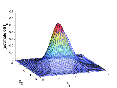
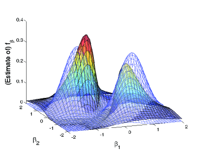
Figure 1. Nonparametric estimator of $f_{\beta}$ for Model 1 (left) and Model 2 (right)

Figure presents the surface plot of the true density (blue mesh) and our estimate (multi-colored surface). Our estimator (4.8) is defined on $\mathbb{S}^{2}$ in this case, and we performed an appropriate transformation to plot it as a density on $\mathbb{R}^{2}$. In the case of model 1, with the reasonable sample size, the location of the peak of the density, as well as its shape, are successfully recovered by our procedure. For model 2, again, our procedure works well: the estimated surface plot nicely captures the locations of the two peaks and their shapes of the true density, thereby exhibiting the underlying mixture structure. While further experimentations are necessary, these results seem to indicate our estimator’s good performance in practical settings.

7. Conclusion

In this paper we have considered nonparametric estimation of a random coefficients binary choice model. By exploiting (previously unnoticed) connections between the model and statistical deconvolution problems and applying results of integral transformation on the sphere, we have developed a new estimator that is practical and possesses desirable statistical properties. It requires neither numerical optimization nor numerical integration, and as such its computational cost is trivial and local maxima and other difficulties in optimization need not be of concern. Its rate of convergence in the L^q norm for all $q\in[1,\infty]$ is derived. Our numerical example suggests that the new procedure works well in finite samples, consistent with its good theoretical properties. It is of great theoretical and practical interest to obtain an adaptive procedure for choosing the smoothing parameters of our estimator, though it is a task we defer to subsequent investigations. With appropriate under-smoothing, the estimator is shown to be asymptotically normal, providing a theoretical basis for nonparametric statistical inference for the random coefficients distribution.

CREST (ENSAE), 3 avenue Pierre Larousse, 92245 Malakoff Cedex, France.

E-mail address: eric.gautier@ensae-paristech.fr

Cowles Foundation for Research in Economics, Yale University, New Haven, CT-06520.

E-mail address: yuichi.kitamura@yale.edu

SUPPLEMENTAL APPENDIX FOR “NONPARAMETRIC ESTIMATION IN RANDOM COEFFICIENTS BINARY CHOICE MODELS”

ERIC GAUTIER AND YUICHI KITAMURA

A.1.1. A Toy Model

As noted in the main text, the key insight for our estimation procedure lies in the fact the estimation of $f_{\beta}$ in (1.3) is mathematically equivalent to a statistical deconvolution problem. To see this, it is useful to first consider the case with $d=2$. We parameterize the vectors $b=\left(b_{1},b_{2}\right)^{\prime}$ and $x=\left(x_{1},x_{2}\right)^{\prime}$ on $\mathbb{S}^{1}$ by their angles $\phi=\arccos\left(b_{1}\right)$ and $\theta=\arccos\left(x_{1}\right)$ in $[0,2\pi)$. As is often the case when Fourier series techniques are used, we consider spaces of complex valued functions. Let ${\rm L}^{p}(\mathbb{S}^{1})$ denote the Banach space of Lebesgue $p$-integrable functions and its norm by $\|\cdot\|_{p}$. In the case of ${{\rm L}^{2}}(\mathbb{S}^{1})$, the norm is derived from the hermitian product $\int_{0}^{2\pi}f(\theta)\overline{g(\theta)}d\theta$. Let $R_{\theta}$ and $f_{\phi}$ denote the extension $R$ of $r$ according to (3.2) and $f_{\beta}$ after the reparameterization. Our task is then to obtain $f_{\phi}$ from the knowledge of $R_{\theta}$. Rewrite (1.3) using these definitions, then divide both sides by $\pi$, to get:

(A.1) $$\frac{R_{\theta}}{\pi}(\theta)=\frac{\mathcal{H}(f_{\beta})}{\pi}(\theta)=\int_{0}^{2\pi}\left(\frac{1}{\pi}\mathbb{I}\left\{|\theta-\phi|<\pi/2\right\}\right)f_{\phi}(\phi)d\phi.$$

If we further define $f_{\theta}:=R_{\theta}/\pi$ and $f_{\eta}(\eta):=\frac{1}{\pi}\mathbb{I}\{|\eta|<\pi/2\}$, then using the standard notation for convolution, (A.1) can be written as $f_{\theta}=f_{\eta}*f_{\phi}$. It is now obvious that the estimation of $f_{\phi}$ (thus $f_{\beta}$) is linked to the following statistical deconvolution problem: unobservable random variables $\phi$ and $\eta$ with densities $f_{\phi}$ and $f_{\eta}$ are related to an observable random variable $\theta$ according to $\theta=\eta+\phi$, and one wishes to recover $f_{\phi}$ from $f_{\theta}$, the density of $\theta$, when $f_{\eta}$ is known (and it is Uniform$[-\pi/2,\pi/2]$ in this case).

The problem of deconvolution on the unit circle can be conveniently solved using Fourier series. The set of functions $\left(\exp(-int)/\sqrt{2\pi}\right)_{n\in{\mathbb{Z}}}$ is the orthonormal basis of ${{\rm L}^{2}}({\mathbb{S}}^{1})$ used to define Fourier series. This system is also complete in ${{\rm L}^{1}}({\mathbb{S}}^{1})$. Reparameterize a function $f\in{{\rm L}^{1}}({\mathbb{S}}^{1})$ it using angles as above, and denote it by $f_{t}$. Denoting the Fourier coefficients of $f\in{{\rm L}^{1}}({\mathbb{S}}^{1})$ by $c_{n}(f_{t})=\int_{0}^{2\pi}f_{t}(t)\exp(-int)dt/(2\pi)$,

(A.2) $$f_{t}(\theta)=\sum_{n\in{\mathbb{Z}}}c_{n}(f_{t})\exp(int)$$

holds in the ${{\rm L}^{1}}({\mathbb{S}}^{1})$ sense. Recall also that for $f$ and $g$ in ${{\rm L}^{1}}({\mathbb{S}}^{1})$, after the same reparameterization,

(A.3) $$c_{n}(f_{t}*g_{t})=2\pi c_{n}(f_{t})c_{n}(g_{t}).$$

Using equation (A.3) we obtain the following proposition.

Proposition A.1.

$c_{0}(R_{\theta})=\pi c_{0}\left(f_{\phi}\right)$ and for $n\in{\mathbb{Z}}\setminus\{0\}$, $c_{n}(R_{\theta})=c_{n}\left(f_{\phi}\right)2\sin\left(n\pi/2\right)/n.$

As in classical deconvolution problems on the real line, our aim is to obtain $f_{t}$ (thus $f_{\beta}$) using equation (A.2) and Proposition A.1. Proposition A.1 shows that $c_{2p}(R_{\theta})=0$ holds for all non-zero $p$’s, regardless of the values of $c_{2p}(f_{\phi}),p\in\mathbb{Z}\backslash\{0\}$. Thus from $r(x)=R_{\theta}(\theta)$ one can only recover the Fourier coefficients $c_{n}(f_{\phi})$ for $n=0$ (which is easily seen to be $1/2\pi$, by integrating both sides of (A.1) and noting that $f_{\beta}$ is a probability density function) and $n=2p+1,p\in\mathbb{Z}$. The same phenomenon occurs in higher dimensions, as explained in Section A.1.3.

Remark A.1.

The vector spaces $H^{2p+1,2}={\rm span}\left\{\exp(i(2p+1)t)/\sqrt{2\pi},\exp(-i(2p+1)t)/\sqrt{2\pi}\right\},p\in\mathbb{N}$ are eigenspaces of the compact self-adjoint operator $\mathcal{H}$ on L${}^{2}(\mathbb{S}^{1})$. These eigenspaces are associated with the eigenvalues $\frac{2(-1)^{p}}{2p+1}$. Also, $\bigoplus_{p\in\mathbb{N}\backslash\{0\}}H^{2p,2}$ is the null space ${\rm ker}\ \mathcal{H}$.

A.1.2. The Gegenbauer polynomials

We summarize some results on the Gegenbauer polynomials, which are used in various parts of the paper. These can be found in Erdélyi et al. (1953) and Groemer (1996). When $\nu=0$ and $d=2$, it is related to the Chebychev polynomials of the first kind, as

$$\forall n\in{\mathbb{N}}\setminus\{0\},\ C_{n}^{0}(t)=\frac{2}{n}T_{n}(t)$$

and

$$C_{0}^{0}(t)=T_{0}(t)=1$$

hold for

$$T_{n}(t)=\cos\left(n\arccos(t)\right),n\in\mathbb{N}.$$

When $\nu=1$ and $d=4$, $C_{n}^{1}(t)$ coincides with the Chebychev polynomial of the second kind $U_{n}(t)$, which is given by

$$U_{n}(t)=\frac{\sin[(n+1)\arccos(t)]}{\sin[\arccos(t)]},n\in\mathbb{N}.$$

The Gegenbauer polynomials are orthogonal with respect to the weight function $(1-t^{2})^{\nu-1/2}dt$ on $[-1,1]$. Note that $C_{0}^{\nu}(t)=1$ and $C_{1}^{\nu}(t)=2\nu t$ for $\nu\neq 0$ while $C_{1}^{0}(t)=2t$. Moreover, the following recursion relation holds

(A.4) $$(n+2)C_{n+2}^{\nu}(t)=2(\nu+n+1)tC_{n+1}^{\nu}(t)-(2\nu+n)C_{n}^{\nu}(t).$$

Implementation of our estimator requires evaluation of the Gegenbauer polynomials for a series of successive values of $n$. The recursion relation (A.4) is therefore a powerful tool. The Gegenbauer polynomials are related to each other through differentiation, that is, they satisfy

(A.5) $$\frac{{\rm d}}{{\rm d}t}C_{n}^{\nu}(t)=2\nu C_{n-1}^{\nu+1}(t)$$

for $\nu>0$ and

(A.6) $$\frac{{\rm d}}{{\rm d}t}C_{n}^{0}(t)=2C_{n-1}^{1}(t).$$

For $\nu\neq 0$ the Rodrigues formula states that

(A.7) $$C_{n}^{\nu}(t)=(-2)^{-n}(1-t^{2})^{-\nu+1/2}\frac{(2\nu)_{n}}{(\nu+1/2)_{n}n!}\frac{{\rm d}^{n}}{{\rm d}t^{n}}(1-t^{2})^{n+\nu-1/2}.$$

The following results are also used in the paper:

(A.8) $$\sup_{t\in[-1,1]}\left|\frac{C_{n}^{\nu}(t)}{C_{n}^{\nu}(1)}\right|\leq 1,$$

(A.9) $$\forall\ \nu>0,\ \forall n\in{\mathbb{N}},\ C_{n}^{\nu}(1)=\left(\begin{array}[]{c}n+2\nu-1\\ n\end{array}\right)$$

(A.10) $$C_{0}^{0}(1)=1\ {\rm and}\ \forall n\in{\mathbb{N}}\setminus\{0\},\ C_{n}^{0}(1)=\frac{2}{n},$$

(A.11) $$C_{n}^{\nu}(-t)=(-1)^{n}C_{n}^{\nu}(t).$$

These orthogonal polynomials are normalized such that

(A.12) $$\|C_{n}^{\nu(d)}\left(x^{\prime}\cdot\right)\|_{2}^{2}=|\mathbb{S}^{d-2}|\int_{-1}^{1}(C_{n}^{\nu(d)}(t))^{2}(1-t^{2})^{(d-3)/2}dt=\frac{|{\mathbb{S}}^{d-1}|(C_{n}^{\nu(d)}(1))^{2}}{h(n,d)}.$$

A.1.3. Tools for Higher Dimensional Spheres

Let us introduce some concepts used for the treatment of the general case $d\geq 2$. We consider functions defined on the sphere ${\mathbb{S}}^{d-1}$, which is a $d-1$ dimensional smooth submanifold in ${\mathbb{R}}^{d}$. The canonical measure on ${\mathbb{S}}^{d-1}$ (or the spherical measure) is denoted by $\sigma$. It is a uniform measure on ${\mathbb{S}}^{d-1}$ satisfying $\int_{{\mathbb{S}}^{d-1}}d\sigma=|{\mathbb{S}}^{d-1}|$, where $|{\mathbb{S}}^{d-1}|$ signifies the surface area of the unit sphere.

Recall that the basis functions $\exp(\pm int)/\sqrt{2\pi}$ are eigenfunctions of $-\frac{{\rm d}}{{\rm d}t^{2}}$ associated with eigenvalue $n^{2}$. In a similar way, the Laplacian on the sphere $\mathbb{S}^{d-1},d\geq 2$, denoted by $\Delta^{S}$, can be used to obtain an orthonormal basis for higher dimensional spheres. It can be defined by the formula

(A.13) $$\Delta^{S}f=(\Delta f\>\check{})\hat{}$$

where $\Delta$ is the Laplacian in $\mathbb{R}^{d}$, $f\check{}$ the radial extension of $f$, that is $f\check{}(x)=f(x/\|x\|)$, and $f\hat{}$ the restriction of $f$ to ${\mathbb{S}}^{d-1}$. Likewise the gradient on the sphere is given by:

(A.14) $$\nabla^{S}f=(\nabla f\>\check{})\hat{}$$

where $\nabla$ is the gradient in $\mathbb{R}^{d}$.

Definition A.1.

A surface harmonic of degree $n$ is the restriction of a homogeneous harmonic polynomial (a homogeneous polynomial $p$ whose Laplacian $\Delta p$ is zero) of degree $n$ in ${\mathbb{R}}^{d}$ to $\mathbb{S}^{d-1}$.

The reader is referred to Müller (1966) and Groemer (1996) for clear and detailed expositions on these concepts and important results concerning spherical harmonics used in this paper. Erdélyi et al. (1953, vol. 2, chapter 9) provide detailed accounts focusing on special functions. Here are some useful results:

Lemma A.1.

The following properties hold:

1. $-\Delta^{S}$ is a positive self-adjoint unbounded operator on ${{\rm L}^{2}}({\mathbb{S}}^{d-1})$, thus it has orthogonal eigenspaces and a basis of eigenfunctions;

2. Surface harmonics of degree $n$ are eigenfunctions of $-\Delta^{S}$ for the eigenvalue $\zeta_{n,d}:=n(n+d-2)$;

3. The dimension of the vector space $H^{n,d}$ of surface harmonics of degree $n$ is

   (A.15) $$h(n,d):=\frac{(2n+d-2)(n+d-2)!}{n!(d-2)!(n+d-2)};$$

4. A system formed of orthonormal bases $(Y_{n,l})_{l=1}^{h(n,d)}$ of $H^{n,d}$ for each degree $n=0,\ldots,\infty$ is complete in ${{\rm L}^{1}}({\mathbb{S}}^{d-1})$, that is, for every $f\in{{\rm L}^{1}}({\mathbb{S}}^{d-1})$ the following equality holds in the ${{\rm L}^{1}}({\mathbb{S}}^{d-1})$ sense:

   $$f=\sum_{n=0}^{\infty}\sum_{l=1}^{h(n,d)}\left(f,Y_{n,l}\right)_{{{\rm L}^{2}}({\mathbb{S}}^{d-1})}Y_{n,l}.$$

Thus $h(n,d)$ is the multiplicity of the eigenvalue $\zeta_{n,d}$, and $H^{n,d}$ is the corresponding eigenspace. Lemma A.1 (i), (ii) and (iv) give the decomposition

$${{\rm L}^{2}}({\mathbb{S}}^{d-1})=\bigoplus_{n\in{\mathbb{N}}}H^{n,d}.$$

The space of surface harmonics of degree 0 is the one dimensional space spanned by $1$. A series expansion on an orthonormal basis of surface harmonics is called a Fourier series when $d=2$, a Laplace series when $d=3$ and in the general case a Fourier-Laplace series.

Orthonormal bases of surface harmonics usually involve parametrization by angles, such as the spherical coordinates when $d=3$ as used by Healy and Kim (1996) or hyperspherical coordinates for $d>3$. Instead, here we work with the decomposition of a function on the spaces $H^{n,d}$ as presented in the next definition so that we avoid specific expressions of basis functions.

Definition A.2.

The condensed harmonic expansion of a function $f$ in ${{\rm L}^{1}}({\mathbb{S}}^{d-1})$ is the series $\sum_{n=0}^{\infty}Q_{n,d}f$, where $Q_{n,d}$ is the projector from L${}^{2}(\mathbb{S}^{d-1})$ to $H^{n,d}$.

This leads to a simple method both in terms of theoretical developments and practical implementations. The projector $Q_{n,d}$ can be expressed as an integral operator with kernel

(A.16) $$q_{n,d}(x,y)=\sum_{l=1}^{h(n,d)}\overline{Y_{n,l}(x)}Y_{n,l}(y),$$

where $(Y_{n,l})_{l=1}^{h(n,d)}$ is any orthonormal basis of $H^{n,d}$. The kernel has a simple expression given by the addition formula:

Theorem A.1 (Addition Formula).

For every $x$ and $y$ $\in\mathbb{S}^{d-1}$, we have

(A.17) $$q_{n,d}(x,y)={}^{\flat}q_{n,d}(x^{\prime}y),\quad{}^{\flat}q_{n,d}(t):=\frac{h(n,d)C_{n}^{\nu(d)}(t)}{|{\mathbb{S}}^{d-1}|C_{n}^{\nu(d)}(1)}$$

where $C_{n}^{\nu}$ are Gegenbauer a and $\nu(d)=(d-2)/2$.

The Sobolev spaces are defined in the Fourier-Laplace domain through the fractional Laplacian defined on a certain subset of ${\rm L}^{p}({\mathbb{S}}^{d-1})$ as

(A.18) $$\left(-\Delta^{S}\right)^{s/2}f:=\sum_{n=0}^{\infty}\zeta_{n,d}^{s/2}Q_{n,d}f.$$

For the case where $p=2$, in stead of the definition of the norm $\|\cdot\|_{p,s}$ given in Section 3 it is also possible to use an equivalent norm, the square of which is equal to

$$\sum_{n=0}^{\infty}\left(1+\zeta_{n,d}\right)^{s}\|Q_{n,d}f\|_{2}^{2}.$$

The following integration by parts holds for functions $f$ in ${\rm H}^{1}({\mathbb{S}}^{d-1})$

(A.19) $$-\int_{{\mathbb{S}}^{d-1}}f(x)\Delta^{S}f(x)d\sigma(x)=\int_{{\mathbb{S}}^{d-1}}\nabla^{S}_{x}f^{\prime}\nabla^{S}_{x}fd\sigma(x)$$

and as a consequence for the second definition of the norm of ${\rm H}^{1}({\mathbb{S}}^{d-1})$ we have

$$\|f\|_{2,1}^{2}=\|f\|_{2}^{2}+\|\nabla^{S}f\|_{2}^{2}.$$

In Section A.1.1 we observed the close relationship between the random coefficients binary choice model and convolution for $d=2$. This connection remains valid in higher dimensions. Suppose a function $f(x,y)$ defined on $\mathbb{S}^{d-1}\otimes\mathbb{S}^{d-1}$ depends on $x$ and $y$ only through the spherical distance $d(x,y)=\arccos(x^{\prime}y)$ (that is, $f$ is a zonal function). Consider the following integral:

$$h(x)=\int_{{\mathbb{S}}^{d-1}}f(x,y)g(y)d\sigma(y):=f\ast g(x),$$

then the function $h$ is a convolution on the sphere. We now see that the choice probability function $r(x)=\mathcal{H}(f_{\beta})(x)=\int_{{\mathbb{S}}^{d-1}}\mathbb{I}\{x^{\prime}b\geq 0\}f_{\beta}(b)d\sigma(b)$ is a special case of $h$ and therefore can also be regarded as convolution. Obtaining $f_{\beta}$ from $r$ (or, inverting $\mathcal{H}$) is therefore a deconvolution problem.

In what follows we often write $f(x,\star)$ when a function $f$ on $\mathbb{S}^{d-1}\otimes\mathbb{S}^{d-1}$ is regarded as a function of $\star$. Also, the notation $\|f(x,\star)\|_{p}$ is used for the L^p norm of $f(x,\star)$, that is, $\|f(x,\star)\|_{p}=\int_{\mathbb{S}^{d-1}}|f(x,y)|^{p}d\sigma(y)$. Note that if $f$ is a zonal function as in the above definition of spherical convolution, its $\mathrm{L}^{p}$ norm $\|f(x,\star)\|_{p}$ does not depend on $x$. The following Young inequalities for convolution on the sphere (see, for example, Kamzolov, 1983) are useful:

Proposition A.2 (Young inequalities).

Suppose $f(x,\star)$ and $g$ belong to ${\rm L}^{r}({\mathbb{S}}^{d-1})$ and ${\rm L}^{p}({\mathbb{S}}^{d-1})$, respectively. Then $h(x)=f\ast g(x)$ is well-defined in ${\rm L}^{q}({\mathbb{S}}^{d-1})$ and

$$\|h\|_{q}\leq\|f\|_{r}\|g\|_{p},$$

where $1\leq p,q,r\leq\infty$ and $\frac{1}{q}=\frac{1}{p}+\frac{1}{r}-1$.

Let $P_{T}$ denote the projection operator onto $\bigoplus_{n=0}^{T}H^{n,d}$, i.e.

(A.20) $$P_{T}f(x)=\sum_{n=0}^{T}Q_{n,d}f(x)=\int_{{\mathbb{S}}^{d-1}}D_{T}(x,y)f(y)d\sigma(y)$$

where

$$D_{T}(x,y)=\sum_{n=0}^{T}q_{n,d}(x,y).$$

The kernel $D_{T}$ extends the classical Dirichlet kernel on the circle to the sphere ${\mathbb{S}}^{d-1}$. The sum over $T$ in the definition of $D_{T}$ also has the simple closed form in terms of derivatives of Gegenbauer polynomials; see Equation (52) in Müller (1966). The linear form $f\rightarrow\int_{{\mathbb{S}}^{d-1}}D_{T}(x,y)f(y)d\sigma(y)$ converges to $\int_{{\mathbb{S}}^{d-1}}f(y)d\delta_{x}(y)=f(x)$ as $T$ goes to infinity, where $\delta_{x}$ denotes the Dirac measure. The Dirichlet kernel yields the best approximation $P_{T}f$ of $f$ in ${{\rm L}^{2}}({\mathbb{S}}^{d-1})$ by polynomials that belong to $\bigoplus_{n=0}^{T}H^{n,d}$, but is known to have flaws. For example, $D_{T}$ does not satisfy

$$\forall f\in{{\rm L}^{1}}({\mathbb{S}}^{d-1}),\lim_{T\rightarrow\infty}\left\|D_{T}*f-f\right\|_{{{\rm L}^{1}}({\mathbb{S}}^{d-1})}=0,$$

that is, the sequence $D_{T},T=0,1,...$ is not an approximate identity (see, e.g., Devroye and Gyorfi 1985) in ${{\rm L}^{1}}({\mathbb{S}}^{d-1})$. Indeed, the ${{\rm L}^{1}}({\mathbb{S}}^{d-1})$ norm of the kernel is not uniformly bounded; more precisely, we have

(A.21) $$\left\|D_{T}(\cdot,x)\right\|_{1}\asymp T^{(d-2)/2}$$

when $d\geq 3$ and

(A.22) $$\left\|D_{T}(\cdot,x)\right\|_{1}\asymp\log T$$

when $d=2$ (as noted above, these norms do not depend on the value of $x\in{\mathbb{S}}^{d-1}$). These bounds can be found in Gronwall (1914) for $d=3$ and Ragozin (1972) and Colzani and Traveglini (1991) for higher dimensions. Also, $D_{T}$ does not have good approximation properties in ${\rm L}^{\infty}({\mathbb{S}}^{d-1})$; in particular, we do not have

$$\forall f\in{\rm L}^{\infty}({\mathbb{S}}^{d-1}),\lim_{T\rightarrow\infty}\left\|D_{T}*f-f\right\|_{{\rm L}^{\infty}({\mathbb{S}}^{d-1})}=0.$$

Near the points of discontinuity of $f$, $D_{T}*f$ has oscillations which do not decay to zero as $T$ grows to infinity, known as the Gibbs oscillations. This phenomenon deteriorates as the dimension increases. These problems can be addressed by using kernels that involves extra smoothing instead of the Dirichlet kernel $D_{T}$. To this end, define a general class of kernel

(A.23) $$K_{T}(x,y)=\sum_{n=0}^{T}\chi(n,T)q_{n,d}(x,y)$$

for some sequence $\chi(n,T)$. These are called smoothed projection kernels. Typically the function $\chi$ is chosen so that it puts more weight on lower frequencies. In particular we impose the following conditions:

Assumption A.1.

1. $\left\|K_{T}(x,\star)\right\|_{1}$ is uniformly bounded in $T$.

2. There exists constants $C$ and $\alpha$ such that for all $x,y,z\in{\mathbb{S}}^{d-1}$,

   $$\left|K_{T}(z,x)-K_{T}(z,y)\right|\leq C\|x-y\|T^{\alpha},$$

   where $\|\cdot\|$ denotes the Euclidean norm.

3. For $p\in[1,\infty]$ and $s>0$, there exists a constant $C$ such that for every $f$ in ${\rm W}_{p}^{s}({\mathbb{S}}^{d-1})$,

   $$\left\|f(\cdot)-\int_{{\mathbb{S}}^{d-1}}K_{T}(\cdot,y)f(y)d\sigma(y)\right\|_{p}\leq CT^{-s}\left\|f\right\|_{p,s}.$$

4. $\chi(\cdot,T)$ takes values in $[0,1]$ and is such that there exists $c>0$ such that for all $0\leq n\leq\lfloor T/2\rfloor$, $\chi\left(n,T\right)\geq c$.

The smoothed projection kernel $K_{T}(x,y)$ depends on $x$ and $y$ only through $d(x,y)$, thus the value of the norm $\left\|K_{T}(x,\star)\right\|_{1}$ in Assumption (i) does not depend on $x\in{\mathbb{S}}^{d-1}$. Assumption (i) could be relaxed, but imposing this on $K_{T}$ allows us to make relatively weak assumptions on the smoothness of the density of the covariates later in this paper. Assumption (ii) is used to establish the $\mathrm{L}^{\infty}$-rates of convergence of our estimators. Assumption (iii) provides bounds for approximation errors. Under this condition, $K_{T}\ast f$ approximates $f\in{\rm L}^{p}({\mathbb{S}}^{d-1})$ with an error of the same order as that of the best $n$-th degree spherical harmonic approximation of a function $f\in{\rm L}^{p}({\mathbb{S}}^{d-1})$ in ${\rm W}_{p}^{s}({\mathbb{S}}^{d-1})$ (see e.g. Kamzolov 1983 and Ditzian 1998). This is useful in our treatment of the bias terms in our estimators. As concrete examples, the following two choices for the weight function $\chi$ in (A.23) satisfy Assumption A.1, as shown in the appendix. The first and the second choices of $\chi$ correspond to the Riesz kernel and the delayed means kernel, respectively.

Proposition A.3.

In the definition of the smoothed kernel (A.23), let

$$\chi(n,T)=\left(1-\left(\frac{\zeta_{n,d}}{\zeta_{T,d}+1}\right)^{s/2}\right)^{l},$$

where $l$ is an integer satisfying $l>(d-2)/2$, or

$$\chi(n,T)=\psi(n/T)$$

where $\psi:\ [0,\infty)\rightarrow[0,\infty)$ is infinitely differentiable, nonincreasing, such that $\psi(x)=1$ if $x\in[0,1]$, $0\leq\Psi(x)\leq 1$ if $x\in[1,2]$, $\psi(x)=0$ if $x\geq 2$. Then $K_{T}$ satisfies Assumption A.1.

The delayed means kernel has the nice property that it does not require prior knowledge of the regularity $s$ in Assumption A.1. The Dirichlet kernel satisfies (ii), (iii) (for $p=2$) and (iv) of Assumption A.1. Like the delayed means kernel, it achieves the optimal rate of approximation without the prior knowledge of $s$.

Proof of Proposition A.3.

First consider the Riesz kernel. (i) follows from (2.4) in Ditzian (1998) and by the fact that Cesàro kernels $C_{h}^{l}$ are uniformly bounded in L${}^{1}(\mathbb{S}^{d-1})$ for $l>\frac{d-2}{2}$ (see, e.g. Bonami and Clerc 1973, p. 225). To show (iii) we use Theorem 4.1 in Ditzian (1998), by letting $P(D)=\Delta^{S}$, $\lambda=\zeta_{T,d}+1=T(T+d-2)+1$, $\alpha=s/2$ and $m=1$. Then it implies an approximation error upper bound $CK_{s/2}(f,\Delta^{S},(\zeta_{T,d}+1)^{-\frac{s}{2}})$, which, in turn, is bounded by $CT^{-s}\|(-\Delta^{S})^{s/2}f\|_{p}$ (see equations (4.2) and (4.1) therein). By the definition of the norm of the Sobolev space $W_{p}^{s}(\mathbb{S}^{d-1})$ (see Definition LABEL:def:sobolev) the result follows. Concerning the delayed means, (i) follows from Theorem 2.2 and Proposition 2.5 of Narcowich et al. (2006). (ii) corresponds to Lemma 2.6 in Narcowich et al. (2006). To see (iii), use Lemma 2.4 (c) in Narcowich et al. (2006) to obtain an upper bound $C\inf_{g\in\bigoplus_{n=0}^{T/2}H^{n,d}}\|f-g\|_{p}$. Let $\lambda=\zeta_{T/2,d}+1=\frac{T}{2}(\frac{T}{2}+d-2)+1$, $\alpha=s/2,m=1,P(D)=\Delta^{S}$ in Ditzian’s (1998) Theorem 6.1, which gives an upper bound on the best spherical harmonic approximation in ${\rm L}^{p}({\mathbb{S}}^{d-1})$ to functions in ${\rm W}_{p}^{s}({\mathbb{S}}^{d-1})$ (see also Kamzolov, 1983), then apply equation (4.1) in Ditzian (1998) again to obtain the desired result. ∎

If the function $f$ is in ${{\rm L}^{2}}({\mathbb{S}}^{d-1})$ then Equations (A.17) and (A.11) imply that $Q_{2p,d}f(x)=Q_{2p,d}f(-x)$ and $Q_{2p+1,d}f(x)=-Q_{2p+1,d}f(-x)$ for $p\in\mathbb{N}$. Consequently, the odd order terms in the condensed harmonic expansions of $f$, $f^{+}$ and $f^{-}$ satisfy $Q_{2p+1}f^{-}=Q_{2p+1}f$ and $Q_{2p+1}f^{+}=0$. Likewise, for the even order terms in the condensed harmonic expansions of these functions $Q_{2p}f^{+}=Q_{2p}f$ and $Q_{2p}f^{-}=0$ hold. We conclude that the sum of the odd order terms in the condensed harmonic expansion corresponds to $f^{-}$ and that of the even order terms to $f^{+}$. As anticipated from the analysis of the $d=2$ case, the operator $\mathcal{H}$ reduces the even part of $f_{\beta}$ to a constant $\frac{1}{2}$, therefore Fourier-Laplace series expansions for $f_{\beta}$ derived later involve only odd order terms.

We now provide a formula that is used to obtain our estimator for $f_{\beta}$. If a non-negative function $f$ has its support included in some hemisphere of $\mathbb{S}^{d-1}$ then

(A.24) $$f(x)=2f^{-}(x)\mathbb{I}\left\{f^{-}(x)>0\right\}.$$

Denote the support of $f$ by ${\rm supp}f$ and let $-{\rm supp}f=\{x|-x\in{\rm supp}f\}$, then this formula follows from the fact that $f^{-}(x)=f^{+}(x)\geq 0$ on ${\rm supp}f$ while $f^{-}(x)=-f^{+}(x)\leq 0$ on $-{\rm supp}f$ and both $f^{-}$ and $f^{+}$ are $0$ on ${\mathbb{S}}^{d-1}\setminus\left({\rm supp}f\bigcup-{\rm supp}f\right)$.

Remark A.2.

If $f$ is a probability density function, the coefficient of degree 0 in the expansion of $f$ on surface harmonics is $1/|{\mathbb{S}}^{d-1}|$. Conversely, any harmonic polynomial or series such that its degree 0 coefficient is $1/|{\mathbb{S}}^{d-1}|$ integrates to one.

The next theorem shows that Fourier-Laplace series on the sphere is a natural tool for the study of the operator $\mathcal{H}$.

Theorem A.2 (Funk-Hecke Theorem).

If $g$ belongs to $H^{n,d}$ for some $n$, and a function $F$ on $(-1,1)$ satisfies

$$\int_{-1}^{1}|F(t)|^{2}(1-t^{2})^{(d-3)/2}dt<\infty,$$

then

(A.25) $$\int_{{\mathbb{S}}^{d-1}}F(x^{\prime}y)g(y)d\sigma(y)=\lambda_{n}(F)g(x)$$

where

$$\lambda_{n}(F)=|\mathbb{S}^{d-2}|C^{\nu(d)}_{n}(1)^{-1}\int_{-1}^{1}F(t)C^{\nu(d)}_{n}(t)(1-t^{2})^{\frac{d-3}{2}}dt.$$

In other words, the kernel operator defined by

$$f\in{{\rm L}^{2}}({\mathbb{S}}^{d-1})\mapsto\ \left(x\mapsto\int_{{\mathbb{S}}^{d-1}}F(x^{\prime}y)f(y)d\sigma(y)\right)\in{{\rm L}^{2}}({\mathbb{S}}^{d-1})$$

is, in the subspace $H^{n,d}$, equivalent to the multiplication by $\lambda_{n}(F)$. Thus a basis of surface harmonics diagonalizes an integral operator if its kernel is a function of the scalar product $x^{\prime}y$.

Remark A.3.

Healy and Kim (1996) use Fourier-Laplace expansions to analyze a deconvolution problem on $\mathbb{S}^{2}$. As we shall see below, the Addition Formula along with condensed harmonic expansions provide a general treatment that works for arbitrary dimensions.

A.1.4. The Hemispherical Transform

The hemispherical transform $\mathcal{H}$, defined by $\mathcal{H}f(x)=\int_{\mathbb{S}^{d-1}}\mathbb{I}\{x^{\prime}y\geq 0\}f(y)d\sigma(y)$, plays a central role in our analysis. It is a special case of the operator considered in the Funk-Hecke theorem above, with $F(t)=\mathbb{I}\{t\in[0,1]\}$, therefore the next proposition follows.

Notation.

We define $\lambda(n,d)=\lambda_{n}\left(\mathbb{I}\left\{t\in[0,1]\right\}\right)$ for $d\geq 3$ and $\lambda(n,2)=\frac{2\sin(n\pi/2)}{n}$.

Proposition A.4.

When $d\geq 2$, the coefficients $\lambda(n,d)$ have the following expressions

1. $\lambda(0,d)=\frac{|{\mathbb{S}}^{d-1}|}{2}$

2. $\lambda(1,d)=\frac{|\mathbb{S}^{d-2}|}{d-1}$

3. $\forall p\in\mathbb{N}\setminus\{0\},\ \lambda(2p,d)=0$

4. $\forall p\in\mathbb{N},\ \lambda(2p+1,d)=\frac{(-1)^{p}|\mathbb{S}^{d-2}|1\cdot 3\cdots(2p-1)}{(d-1)(d+1)\cdots(d+2p-1)}$.

Proof of Proposition A.4.

Define $\alpha(n,d):=C_{n}^{\nu(d)}(1)|\mathbb{S}^{d-2}|^{-1}\lambda_{n}\left(\mathbb{I}\left\{t\in[0,1]\right\}\right)$. By the Funk-Hecke theorem

$$\alpha(n,d)=\int_{0}^{1}C_{n}^{\nu(d)}(t)(1-t^{2})^{(d-3)/2}dt,$$

thus using (A.7),

$$\alpha(n,d)=\frac{(-2)^{-n}(d-2)_{n}}{n!\left((d-1)/2\right)_{n}}\int_{0}^{1}\frac{{\rm d}^{n}}{{\rm d}t^{n}}(1-t^{2})^{n+(d-3)/2}dt.$$

Therefore for $n\geq 1$ and $d\geq 3$,

$$\alpha(n,d)=-\frac{(-2)^{-n}(d-2)_{n}}{n!\left((d-1)/2\right)_{n}}\left.\frac{{\rm d}^{n-1}}{{\rm d}t^{n-1}}(1-t^{2})^{n-1+(d-3)/2}dt\right|_{t=0}$$

since the term on the right hand-side is equal to 0 for $t=1$. To prove that the coefficients $\alpha(2p,d)$ are equal to zero for $p$ positive it is enough to prove

$$\left.\frac{{\rm d}^{2p+1}}{{\rm d}t^{2p+1}}(1-t^{2})^{2p+1+m}\right|_{t=0}=0,\quad\forall m\geq 1,\ p\geq 0.$$

The Faá di Bruno formula gives that this quantity is equal to

$$\left.\sum_{k_{1}+2k_{2}=2p+1}\frac{(-1)^{2p+1-k_{2}}(2p+1)!(m+1)\cdots(2p+1+m)}{k_{1}!k_{2}!}(1-t^{2})^{m+k_{2}}(2t)^{k_{1}}\right|_{t=0}.$$

and the result follows since $k_{1}$ in the sum cannot be equal to 0.

When $n=2p+1$ for $p\in\mathbb{N}$ we obtain, again using the Faá di Bruno formula, that the derivative at $t=0$ is equal to

$$(-1)^{p}\frac{(2p)!}{p!}\left[(2p+1+(d-3)/2)(2p+(d-3)/2)\cdots(p+2+(d-3)/2)\right].$$

Together with (A.9), the desired result follows. For the case $d=2$ we use Proposition A.1. ∎

Define ${\rm L}_{{\rm odd}}^{2}({\mathbb{S}}^{d-1})$ and ${\rm H}_{{\rm odd}}^{s}({\mathbb{S}}^{d-1})$ as the restrictions of ${{\rm L}^{2}}({\mathbb{S}}^{d-1})$ and ${\rm H}^{s}({\mathbb{S}}^{d-1})$ to odd functions and similarly ${\rm L}_{{\rm even}}^{2}({\mathbb{S}}^{d-1})$ and ${\rm H}_{{\rm even}}^{s}({\mathbb{S}}^{d-1})$ for even functions. The following corollary is a direct consequence of the Funk-Hecke Theorem and Proposition A.4, and corresponds to an observation made in Remark A.1 for the $d=2$ case.

Corollary A.1.

The null space of the hemispherical transform $\mathcal{H}$ is given by

$${\rm ker}\ \mathcal{H}=\bigoplus_{p=1}^{\infty}H^{2p,d}=\left\{f\in{\rm L}_{{\rm even}}^{2}({\mathbb{S}}^{d-1}):\ \int_{{\mathbb{S}}^{d-1}}f(x)d\sigma(x)=0\right\},$$

when $\mathcal{H}$ is viewed as an operator on ${{\rm L}^{2}}({\mathbb{S}}^{d-1})$. The spaces $H^{0,d}$ and $H^{2p+1,d}$ for $p\in\mathbb{N}$ are the eigenspaces associated with the non-zero eigenvalues of $\mathcal{H}$.

As a consequence of Proposition A.4, $\mathcal{H}$ is not injective and restrictions have to be imposed in order to ensure identification of $f_{\beta}$. Section 3 presents sufficient conditions that allows us to reconstruct $f_{\beta}$ from $f_{\beta}^{-}$.

The following proposition can be found in Rubin (1999).

Proposition A.5.

$\mathcal{H}$ is a bijection from ${\rm L}_{{\rm odd}}^{2}({\mathbb{S}}^{d-1})$ to ${\rm H}_{{\rm odd}}^{d/2}({\mathbb{S}}^{d-1})$.

Lemma A.2.

(A.26) $$h(n,d) \asymp n^{d-2},$$

(A.27) $$|\lambda(2p+1,d)| \asymp p^{-d/2}.$$

Proof.

Estimate (A.26) is clearly satisfied when $d=2$ and $3$ since $h(n,2)=2$ and $h(n,3)=2n+1$. When $d\geq 4$ we have

$$h(n,d)=\frac{2}{(d-2)!}(n+(d-2)/2)[(n+1)(n+2)\cdots(n+d-3)],$$

and the results follow.
Next we turn to (A.27). When $d$ is even and $p\geq d/2$

$$|\lambda(2p+1,d)|=\frac{\kappa_{d}}{(2p+1)(2p+3)\cdots(2p+d-1)}$$

where

$$\kappa_{d}=\frac{|\mathbb{S}^{d-2}|1\cdot 3\cdots(d-1)}{d-1}$$

and (A.27) follows. Sterling’s double inequality (see Feller (1968) p.50-53), that is,

$$\sqrt{2\pi}n^{n+1/2}\exp\left(-n+\frac{1}{12n+1}\right)<n!<\sqrt{2\pi}n^{n+1/2}\exp\left(-n+\frac{1}{12n}\right),$$

implies that

$$\frac{(2^{p}p!)^{2}}{(2p)!}\asymp\sqrt{p}$$

and therefore

$$1\cdot 3\cdots(2p-1)\asymp\sqrt{p}2\cdot 4\cdots(2p).$$

Thus for $p\geq d/2$ and $d$ odd we have

$$|\lambda(2p+1,d)|\asymp\frac{\sqrt{p}}{(2p+2)(2p+4)\cdots(2p+d-1)}$$

and (A.27) holds for both even and odd $d$. ∎

We can now easily check that

Proposition A.6.

For all $s>0$, there exists positive constants $C_{l}$ and $C_{u}$ such that for all $f$ in ${\rm H}^{s}({\mathbb{S}}^{d-1})$

$$C_{l}\left\|f^{-}\right\|_{2,s}\leq\left\|\mathcal{H}(f^{-})\right\|_{2,s+d/2}\leq C_{u}\left\|f^{-}\right\|_{2,s}.$$

Proof of Proposition A.6.

By definition we have

$$\|\mathcal{H}\left(f^{-}\right)\|_{2,s+d/2}^{2}=\sum_{p=0}^{\infty}(1+\zeta_{2p+1,d})^{s+d/2}\|Q_{2p+1,d}\mathcal{H}(f^{-})\|_{2}^{2}$$

where according to the Funk-Hecke Theorem

$$Q_{2p+1,d}\mathcal{H}(f^{-}) =Q_{2p+1,d}\mathcal{H}\left(\sum_{q=0}^{\infty}Q_{2q+1,d}f\right)$$

$$=Q_{2p+1,d}\left(\sum_{q=0}^{\infty}\lambda(2q+1,d)Q_{2q+1,d}f\right)$$

$$=\lambda(2p+1,d)Q_{2p+1,d}f.$$

The result follows since Lemma A.2 implies that $(1+\zeta_{2p+1,d})^{s+d/2}\lambda^{2}(2p+1,d)\asymp(1+\zeta_{2p+1,d})^{s}$. ∎

The factor $d/2$ in Proposition A.6 corresponds to the degree of “regularization” due to smoothing by $\mathcal{H}$. Now the inverse of an odd function $f^{-}$ is given by

(A.28) $$\mathcal{H}^{-1}(f^{-})(y)=\sum_{p=0}^{\infty}\frac{1}{\lambda(2p+1,d)}\int_{\mathbb{S}^{d-1}}q_{2p+1,d}(x,y)f^{-}(x)d\sigma(x).$$

This is straightforward given our results at hand: for example, operate $\mathcal{H}$ on the RHS to see:

$$\mathcal{H}\left(\sum_{p=0}^{\infty}\frac{1}{\lambda(2p+1,d)}\int_{\mathbb{S}^{d-1}}q_{2p+1,d}(x,y)f^{-}(x)d\sigma(x)\right) =\sum_{p=0}^{\infty}\frac{1}{\lambda(2p+1,d)}\mathcal{H}Q_{2p+1,d}f^{-}$$

$$=\sum_{p=0}^{\infty}\frac{\lambda(2p+1,d)}{\lambda(2p+1,d)}Q_{2p+1,d}f^{-}\ \text{(by the Funk-Hecke Theorem)}$$

$$=f^{-}.$$

If $f^{-}$ belongs to ${\rm H}^{d/2}({\mathbb{S}}^{d-1})$, then $\mathcal{H}^{-1}(f^{-})(b)$ is a well-defined ${{\rm L}^{2}}({\mathbb{S}}^{d-1})$ function. Otherwise it should be understood as a distribution and is only defined in a Sobolev space with negative exponent. Moreover, if $d$ is a multiple of 4, it is possible to relate the inverse of the operator $\mathcal{H}$ with differentiation as in the case of $d=2$:

Proposition A.7.

If $d$ is a multiple of 4,

$$\mathcal{H}^{-1}=|\mathbb{S}^{d-2}|\prod_{k=1}^{d/4}[-\Delta^{S}+2(k-1)(d-2k)].$$

Proof of Proposition A.7.

If we consider the case where $d$ is even, we know from Proposition A.4, that

$$\frac{1}{\lambda(2p+1,d)}=(-1)^{p}|\mathbb{S}^{d-2}|(2p+1)(2p+3)\ldots(d+2p-1).$$

Thus if $d$ is a multiple of 4,

$$\frac{1}{\lambda(2p+1,d)}=|\mathbb{S}^{d-2}|\prod_{k=1}^{d/4}[-\zeta_{2p+1,d}+2(k-1)(d-2k)].$$

Using this and (4.1),

$$\mathcal{H}^{-1} =\sum_{p=0}^{\infty}\frac{1}{\lambda(2p+1,d)}Q_{2p+1,d}$$

$$=\sum_{p=0}^{\infty}|\mathbb{S}^{d-2}|\left(\prod_{k=1}^{d/4}[-\zeta_{2p+1,d}+2(k-1)(d-2k)]\right)Q_{2p+1,d}.$$

Recall (A.18) and the proposition is proved. ∎

This connection between the inverse of $\mathcal{H}$ and differentiation suggests that a Bernstein-type inequality might hold for $\mathcal{H}^{-1}$. Indeed, even though the above inversion formula is concerned with $d$’s that are multiples of 4, the following Bernstein inequality holds for every dimension.

Theorem A.3 (Bernstein inequality).

For every $d\geq 2$ and every $q\in[1,\infty]$, there exists a positive constant $B(d,q)$ such that for all $P$ in $\bigoplus_{p=0}^{T}H^{2p+1,d}$,

(A.29) $$\|\mathcal{H}^{-1}P\|_{q}\leq B(d,q)T^{d/2}\|P\|_{q}.$$

Proof of Theorem A.3.

We can write

$$\mathcal{H}^{-1}=P_{1}(D)-P_{2}(D)$$

where $P_{1}(D)$ and $P_{2}(D)$ are defined for all odd function $f^{-}$ by

$$P_{1}(D)f^{-} =\sum_{p=0}^{\infty}\frac{1}{\lambda(4p+3)}\int_{{\mathbb{S}}^{d-1}}q_{4p+3}(x,y)f^{-}(x)d\sigma(x)$$

$$P_{2}(D)f^{-} =-\sum_{p=0}^{\infty}\frac{1}{\lambda(4p+1)}\int_{{\mathbb{S}}^{d-1}}q_{4p+1}(x,y)f^{-}(x)d\sigma(x).$$

$P_{1}(D)$ and $P_{2}(D)$ are two unbounded operators on $B={\rm L}_{{\rm odd}}^{q}({\mathbb{S}}^{d-1})$ with non-positive eigenvalues. We apply Theorem 3.2. of Ditzian (1998) to $-P_{1}(D)$ and $-P_{2}(D)$ choosing $\alpha=1$. Condition (1.6) of Ditzian (1998) can be verified using Proposition 2.2 with $r=1$ and $p=q$ and the fact that for the Cesaro kernels $C_{h}^{l}$ are uniformly bounded in L${}^{1}(\mathbb{S}^{d-1})$ for $l>\frac{d-2}{2}$ (see, e.g. Bonami and Clerc, 1973). We see, using the triangle inequality, that for all $P$ in $\bigoplus_{p=0}^{T}H^{2p+1,d}$,

$$\|\mathcal{H}^{-1}P\|_{q} \leq C\frac{1}{\lambda^{2}(2T+1,d)}\|P\|_{q}$$

$$\leq CT^{d}\|P\|_{q}.$$

The last inequality follows from (A.27). ∎

Rubin (1999) gives other inversion formulas for the Hemispherical transform in terms of differential operators. The fact that the inversion roughly corresponds to differentiation is another manifestation of the ill-posedness of our problem at hand. The inverse operator $\mathcal{H}^{-1}$ is indeed unbounded. We call the factor $d/2$ in (A.29) the degree of ill-posedness of the inverse problem. For the case $q=2$, there exists a lower bound for $\|\mathcal{H}^{-1}P\|_{q}$ in (A.29) of order $T^{d/2}$ as well, implying that the upper bound $T^{d/2}$ in the order of $T$ obtained in Theorem A.3 is tight.

A.1.5. Estimators for the Choice Probability Function

This section considers estimation of the choice probability function $r$ and its extension $R$. We propose an estimator for $r$, which, in turn, yields a computationally simple estimator for $f_{\beta}$. Also the asymptotic results presented here are useful for the next section where we study the limiting properties of our estimator for the random coefficients density $f_{\beta}$.

Since $R$ is square integrable on ${\mathbb{S}}^{d-1}$, it has a condensed harmonic expansion which enables us to obtain the expressions in the next theorem.

Theorem A.4.

For $x$ in ${\mathbb{S}}^{d-1}$, we have

(A.30) $$R(x)=\frac{1}{2}+\sum_{p=0}^{\infty}{\mathbb{E}}\left[\frac{(2Y-1)}{f_{X}(X)}q_{2p+1,d}(X,x)\right].$$

This suggests an estimator of the form $\hat{R}_{1}(x)=\frac{1}{2}+\hat{R}^{-}_{1}$ with

$$\hat{R}^{-}_{1}(x)=\frac{1}{N}\sum_{i=1}^{N}\frac{(2y_{i}-1)}{\hat{f}_{X}(x_{i})}\sum_{p=0}^{T_{N}}q_{2p+1,d}(x_{i},x)$$

where $\hat{f}_{X}$ is an estimator of $f_{X}$ and $T_{N}$ is a suitably chosen sequence diverging to infinity with $N$. Note that the second summation corresponds to the Dirichlet kernel. We can generalize this, by introducing a class of estimators of the form

(A.31) $$\hat{R}^{-}_{2}(x)=\frac{1}{N}\sum_{i=1}^{N}\frac{(2y_{i}-1)}{\hat{f}_{X}(x_{i})}K_{2T_{N}}^{-}(x_{i},x)$$

where $K_{2T_{N}}^{-}$ is the odd part of a kernel of the form (A.23) satisfying Assumption A.1, such as the two kernels in Proposition A.3.

The estimator (A.31) is convenient, though the plug-in term $\hat{f}_{X}$ has to be treated with care. We avoid restrictive assumptions on the distributions of covariates and allow $f_{X}(x)$ to decay to zero as $x$ approaches the boundary of its support $H^{+}$. To deal with the latter problem, we modify (A.31) by

(A.32) $$\hat{R}^{-}(x)=\frac{1}{N}\sum_{i=1}^{N}\frac{(2y_{i}-1)K_{2T_{N}}^{-}(x_{i},x)}{\max\left(\hat{f}_{X}(x_{i}),m_{N}\right)}$$

where $m_{N}$ is a trimming factor going to 0 with the sample size. Our estimator for $R$ is then

(A.33) $$\widehat{R}=\frac{1}{2}+\hat{R}^{-}.$$

Remark A.4.

Alternative estimators of $R^{-}$ are available. For example, one may use kernel regression on the sphere to estimate $r$ in order to obtain an estimator for $R^{-}$. As noted before, however, we then need to use numerical integration to evaluate (4.5) to calculate $\hat{f}_{\beta}^{-}$.

Proof of Theorem A.4.

$R$ has the following condensed harmonic expansion

$$R(x)=\frac{1}{2}+\sum_{p=1}^{\infty}(Q_{2p+1,d}R)(x).$$

We then write using (3.2), changing variables and using (A.11),

$$(Q_{2p+1,d}R)(x) =\int_{{\mathbb{S}}^{d-1}}q_{2p+1,d}(x,z)R(z)d\sigma(z)$$

$$=\int_{H^{+}}q_{2p+1,d}(x,z)r(z)d\sigma(z)+\int_{H^{-}}q_{2p+1,d}(x,z)(1-r(-z))d\sigma(z)$$

$$=\int_{H^{+}}q_{2p+1,d}(x,z)r(z)d\sigma(z)-\int_{H^{+}}q_{2p+1,d}(x,z)(1-r(z))d\sigma(z)$$

$$=\int_{H^{+}}q_{2p+1,d}(x,z)(2r(z)-1)d\sigma(z)$$

$$=\int_{H^{+}}q_{2p+1,d}(x,z){\mathbb{E}}\left[\left.\frac{2Y-1}{f_{X}(z)}\right|X=z\right]f_{X}(z)d\sigma(z)$$

$$={\mathbb{E}}\left[\frac{(2Y-1)q_{2p+1,d}(x,X)}{f_{X}(X)}\right].$$

∎

A.1.6. Proofs of Main Results

Proof of Proposition 3.1.

It is straightforward that the model (1.1) and Assumption 1.1 imply that the choice probability function $r$ given by (1) is homogeneous of degree 0. Proposition A.5 along with the fact that $R=\frac{1}{2}+\mathcal{H}\left(f_{\beta}^{-}\right)$ with $f_{\beta}^{-}\in{\rm L}_{\mathrm{odd}}^{2}({\mathbb{S}}^{d-1})$ implies that $R$ belongs to ${\rm H}^{d/2}({\mathbb{S}}^{d-1})$. We now turn to the proof of sufficiency. If the extension $R$ given by (3.2) belongs to ${\rm H}^{d/2}({\mathbb{S}}^{d-1})$ then so does $R^{-}$ and Proposition A.5 shows that there exists a unique odd function $f^{-}$ in ${{\rm L}^{2}}({\mathbb{S}}^{d-1})$ such that

$$R=\frac{1}{2}+\mathcal{H}\left(f^{-}\right)=\mathcal{H}\left(\frac{1}{|{\mathbb{S}}^{d-1}|}+f^{-}\right).$$

Moreover, since $0\leq R(x)\leq 1$ holds for every $x\in\mathbb{S}^{d-1}$, the above relationship implies that $\frac{1}{2}\geq\mathcal{H}f^{-}(x),\forall x\in\mathbb{S}^{d-1}$. But $\mathcal{H}f^{-}(x)\geq\int_{\{f^{-}(b)\geq 0\}}f^{-}(b)d\sigma(b)$ holds for some $x$. Therefore we conclude that $\frac{1}{2}\geq\int_{\{f^{-}(b)\geq 0\}}f^{-}(b)d\sigma(x)=-\int_{\{f^{-}(b)\leq 0\}}f^{-}(b)d\sigma(b)$, thus $\int_{{\mathbb{S}}^{d-1}}|f^{-}(b)|d\sigma(b)\leq 1$. Also, following the discussion in Section A.1.3, $\frac{1}{|{\mathbb{S}}^{d-1}|}+f^{-}$ integrates to 1. We have seen in Corollary A.1 that for even function $g$ that has 0 as the coefficient of degree 0 in its expansion on the surface harmonics (i.e. an even function that integrates to zero over the sphere),

$$R=\mathcal{H}\left(g+\frac{1}{|{\mathbb{S}}^{d-1}|}+f^{-}\right)$$

holds. Now consider

$$g=|f^{-}|-\frac{1}{|{\mathbb{S}}^{d-1}|}\int_{{\mathbb{S}}^{d-1}}|f^{-}(b)|d\sigma(b),$$

then this certainly is even and integrates to zero. Using this, define

$$f_{\beta}^{*}:=g+\frac{1}{|{\mathbb{S}}^{d-1}|}+f^{-}=2f^{-}\mathbb{I}\{f^{-}>0\}+\frac{1}{|{\mathbb{S}}^{d-1}|}\left(1-\int_{{\mathbb{S}}^{d-1}}|f^{-}(b)|d\sigma(b)\right)\geq 0.$$

Obviously ${f_{\beta}^{*}}^{-}=f^{-}$. This function $f_{\beta}^{*}$ is non-negative and integrates to one, and thus it is a proper probability density function (pdf). It is indeed bounded from below by $\frac{1}{|{\mathbb{S}}^{d-1}|}\left(1-\int_{{\mathbb{S}}^{d-1}}|f^{-}(b)|d\sigma(b)\right)$. As a consequence, there exists a pdf $f_{\beta}^{*}$ such that

$$R=\mathcal{H}\left(f_{\beta}^{*}\right)=\frac{1}{2}+\mathcal{H}\left({f_{\beta}^{*}}^{-}\right)$$

and for all $x$ in $H^{+}$, $r(x)=\mathcal{H}\left(f_{\beta}^{*}\right)(x)$. ∎

Proof of Theorem 4.1.

We use the shorthand notation $\mathbb{I}(b):=\mathbb{I}\{f_{\beta}^{-}(b)>0\}$ and $\hat{\mathbb{I}}(b):=\mathbb{I}\{\hat{f}_{\beta}^{-}(b)>0\}$. Then $f_{\beta}=2f^{-}_{\beta}\mathbb{I}$ and $\hat{f}_{\beta}=2\hat{f}^{-}_{\beta}\hat{\mathbb{I}}$. We write

$$\overline{f}_{\beta,T}^{\ -}(b) =\frac{1}{N}\sum_{i=1}^{N}\frac{(2y_{i}-1)\mathcal{H}^{-1}\left(K_{2T_{N}}^{-}(x_{i},\cdot)\right)(b)}{\max\left(f_{X}(x_{i}),m_{N}\right)}$$

$$\overline{f}_{\beta}^{\ -}(b) =\frac{1}{N}\sum_{i=1}^{N}\frac{(2y_{i}-1)\mathcal{H}^{-1}\left(K_{2T_{N}}^{-}(x_{i},\cdot)\right)(b)}{f_{X}(x_{i})}$$

and use the decomposition

(A.34) $$\hat{f}_{\beta}^{-}-f_{\beta}^{-}=\left(\hat{f}_{\beta}^{-}-\overline{f}_{\beta,T}^{\ -}\right)+\left(\overline{f}_{\beta,T}^{\ -}-{\mathbb{E}}\left[\overline{f}_{\beta,T}^{\ -}\right]\right)+\left({\mathbb{E}}\left[\overline{f}_{\beta,T}^{\ -}\right]-{\mathbb{E}}\left[\overline{f}_{\beta}^{\ -}\right]\right)+\left({\mathbb{E}}\left[\overline{f}_{\beta}^{\ -}\right]-f_{\beta}^{-}\right),$$

and denote the terms on the right hand side by $S_{\mathrm{p}}$ (stochastic component due to plug-in), $S_{\mathrm{e}}$ (stochastic component of the infeasible estimator $\overline{f}_{\beta,T}^{\ -}$), $B_{\mathrm{t}}$ (trimming bias) and $B_{\mathrm{a}}$ (approximation bias).

Take $q\in[1,\infty)$,

$$\|\hat{f}_{\beta}-f_{\beta}\|_{q}^{q}= \int(\hat{f}_{\beta}(b)-f_{\beta}(b))^{q}d\sigma(b)$$

$$= \int_{\mathbb{I}(b)=1,\hat{\mathbb{I}}(b)=1}(\hat{f}_{\beta}(b)-f_{\beta}(b))^{q}d\sigma(b)+\int_{\mathbb{I}(b)=0,\hat{\mathbb{I}}(b)=1}(\hat{f}_{\beta}(b)-f_{\beta}(b))^{q}d\sigma(b)$$

$$+\int_{\mathbb{I}(b)=1,\hat{\mathbb{I}}(b)=0}(\hat{f}_{\beta}(b)-f_{\beta}(b))^{q}d\sigma(b)+\int_{\mathbb{I}(b)=0,\hat{\mathbb{I}}(b)=0}(\hat{f}_{\beta}(b)-f_{\beta}(b))^{q}d\sigma(b)$$

$$:= A_{1}+A_{2}+A_{3}+A_{4}.$$

Obviously

$$A_{1}=\int_{\mathbb{I}(b)=1,\hat{\mathbb{I}}(b)=1}(2\hat{f}^{-}_{\beta}(b)-2f^{-}_{\beta}(b))^{q}d\sigma(b)$$

and $A_{4}=0$. Also,

$$A_{2}=\int_{\mathbb{I}(b)=0,\hat{\mathbb{I}}(b)=1}(2\hat{f}^{-}_{\beta}(b)-f_{\beta}(b))^{q}d\sigma(b).$$

But given ${\mathbb{I}}(b)=0$ and $\hat{\mathbb{I}}(b)=1$, $2\hat{f}^{-}_{\beta}(b)>0$, $f_{\beta}(b)=0$ and $2f^{-}_{\beta}(b)\leq 0$, so replacing $f_{\beta}$ with $2f^{-}_{\beta}$ in the bracket,

$$A_{2}\leq\int_{\mathbb{I}(b)=0,\hat{\mathbb{I}}(b)=1}(2\hat{f}^{-}_{\beta}(b)-2f^{-}_{\beta}(b))^{q}d\sigma(b).$$

Similarly,

$$A_{3}=\int_{\mathbb{I}(b)=1,\hat{\mathbb{I}}(b)=0}(\hat{f}_{\beta}(b)-2f^{-}_{\beta}(b))^{q}d\sigma(b).$$

and given ${\mathbb{I}}(b)=1$ and $\hat{\mathbb{I}}(b)=0$, $2f^{-}_{\beta}(b)>0$, $\hat{f}_{\beta}(b)=0$ and $2\hat{f}^{-}_{\beta}(b)\leq 0$, so replacing $f_{\beta}$ with $2f^{-}_{\beta}$ in the bracket,

$$A_{3}\leq\int_{\mathbb{I}(b)=0,\hat{\mathbb{I}}(b)=1}(2\hat{f}^{-}_{\beta}(b)-2f^{-}_{\beta}(b))^{q}d\sigma(b).$$

Overall,

$$\|\hat{f}_{\beta}-f_{\beta}\|_{q}^{q}\leq 2^{q}\|\hat{f}^{-}_{\beta}-f^{-}_{\beta}\|_{q}^{q}.$$

A similar proof can be carried out replacing ${\rm L}^{q}({\mathbb{S}}^{d-1})$ by ${\rm L}^{\infty}({\mathbb{S}}^{d-1})$. Thus it is enough to consider the behavior of $\hat{f}^{-}_{\beta}-f^{-}_{\beta}$ instead of $\hat{f}_{\beta}-f_{\beta}$. As noted above, the former can be decomposed into four terms, $S_{\mathrm{p}}$, $S_{\mathrm{e}}$, $B_{\mathrm{t}}$ and $B_{\mathrm{a}}$.

We start with the analysis of $S_{\mathrm{p}}$. Note that for $q\in[1,\infty]$

$$\|S_{\mathrm{p}}\|_{q} =\left\|\mathcal{H}^{-1}\left(\frac{1}{N}\sum_{i=1}^{N}\frac{(2y_{i}-1)K_{2T_{N}}^{-}(x_{i},\cdot)}{\max(f_{X}(x_{i}),m_{N})}\left(\frac{\max\left(f_{X}(x_{i}),m_{N}\right)}{\max\left(\hat{f}_{X}(x_{i}),m_{N}\right)}-1\right)\right)\right\|_{q}$$

$$\leq B(d,q)T_{N}^{d/2}\left\|\frac{1}{N}\sum_{i=1}^{N}\frac{(2y_{i}-1)K_{2T_{N}}^{-}(x_{i},\cdot)}{\max(f_{X}(x_{i}),m_{N})}\left(\frac{\max\left(f_{X}(x_{i}),m_{N}\right)}{\max\left(\hat{f}_{X}(x_{i}),m_{N}\right)}-1\right)\right\|_{q}\quad{\rm(by\ Theorem\ \ref{tbernstein})}$$

$$\leq B(d,q)T_{N}^{d/2}m_{N}^{-1}\left\|\frac{1}{N}\sum_{i=1}^{N}\left|K_{2T_{N}}(x_{i},\cdot)\right|\right\|_{q}\max_{i=1,\ldots,N}\left|\frac{\max\left(f_{X}(x_{i}),m_{N}\right)}{\max\left(\hat{f}_{X}(x_{i}),m_{N}\right)}-1\right|$$

$$\leq B(d,q)T_{N}^{d/2}m_{N}^{-2}\left\|\frac{1}{N}\sum_{i=1}^{N}\left|K_{2T_{N}}(x_{i},\cdot)\right|\right\|_{q}\max_{i=1,\ldots,N}\left|f_{X}(x_{i})-\hat{f}_{X}(x_{i})\right|$$

holds, where we have used the triangle inequality. The ${\rm L}^{q}$-norm on the right hand side is bounded from above by

(A.35) $$\left\|\frac{1}{N}\sum_{i=1}^{N}\left|K_{2T_{N}}(x_{i},\cdot)\right|-{\mathbb{E}}\left|K_{2T_{N}}(X,\cdot)\right|\right\|_{q}+\left\|{\mathbb{E}}\left|K_{2T_{N}}(X,\cdot)\right|\right\|_{q}:=\|T_{1}\|_{q}+\|T_{2}\|_{q}.$$

First consider the term $\|T_{1}\|_{q}$. We begin with the case of $q\in[1,2]$. By the Hölder inequality,

$${\mathbb{E}}\left[\|T_{1}\|_{q}^{q}\right] =\int_{{\mathbb{S}}^{d-1}}{\mathbb{E}}\left[T_{1}(x)^{q}\right]d\sigma(x)$$

$$\leq\int_{{\mathbb{S}}^{d-1}}{\mathbb{E}}\left[T_{1}(x)^{2}\right]^{q/2}d\sigma(x)$$

where

(A.36) $${\mathbb{E}}\left[T_{1}(x)^{2}\right] \leq\frac{1}{N}{\mathbb{E}}\left[\left(K_{2T_{N}}(X,x)\right)^{2}\right]$$

$$\leq\frac{C}{N}\left\|K_{2T_{N}}(\star_{2},x)\right\|_{2}^{2}\quad(\text{boundedness assumption on }f_{X})$$

$$=\frac{C}{N}\left\|\sum_{n=0}^{2T_{N}}\chi(n,2T_{N})q_{n,d}(\star_{2},x)\right\|_{2}^{2}$$

$$\leq\frac{C}{N}\sum_{n=0}^{2T_{N}}\left\|q_{n,d}(\star_{2},x)\right\|_{2}^{2}\quad(\text{by Assumption \ref{asskernel}(\ref{k4})})$$

$$\leq\frac{C}{N}\sum_{n=0}^{2T_{N}}\frac{h^{2}(n,d)\left\|C_{n}^{\nu(d)}(\star_{2}^{\prime}x)\right\|_{2}^{2}}{|\mathbb{S}^{d-1}|^{2}(C_{n}^{\nu(d)}(1))^{2}}$$

$$\leq\frac{C}{N}\sum_{n=0}^{2T_{N}}h(n,d)\quad{\rm(by\ \eqref{emass})}$$

$$\leq\frac{CT_{N}^{d-1}}{N}\quad{\rm(by\ Lemma\ \ref{l1})}.$$

By the Markov inequality,

(A.37) $$T_{N}^{d/2}m_{N}^{-2}\|T_{1}\|_{q}=O_{p}\left(m_{N}^{-2}N^{-1/2}T_{N}^{(2d-1)/2}\right),$$

providing a convergence rate for $\|T_{1}\|_{q},q\in[1,2]$. So if we can establish a similar rate for $\|T_{1}\|_{\infty}$, all ${\rm L}^{q}({\mathbb{S}}^{d-1})$ convergence rates of $T_{1}$ for $q\in(2,\infty]$ can be interpolated between the ${{\rm L}^{2}}({\mathbb{S}}^{d-1})$ and ${\rm L}^{\infty}({\mathbb{S}}^{d-1})$ convergence rates using the following inequality:

(A.38) $$\forall f\in{\rm L}^{\infty}({\mathbb{S}}^{d-1}),\ \|f\|_{q}\leq\|f\|_{2}^{2/q}\|f\|_{\infty}^{1-2/q}.$$

To see this, note

$$\|f\|_{q} =\|f^{2}|f|^{q-2}\|_{1}^{1/q}$$

$$\leq\left[\|f^{2}\|_{1}\||f|^{q-2}\|_{\infty}\right]^{1/q}\quad\text{(by H\"{o}lder)}$$

$$=\|f\|_{2}^{2/q}\|f\|_{\infty}^{1-2/q}.$$

We can thus focus on $\|T_{1}\|_{\infty}$. We cover the sphere $\mathbb{S}^{d-1}$ by $\mathfrak{N}(N,r,d)$ geodesic balls (caps) $\left(B_{i}\right)_{i=1}^{\mathfrak{N}(N,r,d)}$ of centers $\left(\tilde{x}_{i}\right)_{i=1}^{\mathfrak{N}(N,r,d)}$ and radius $R(N,r,d)$, that is, $B_{i}=\{x\in{\mathbb{S}}^{d-1}:\ \|x-\tilde{x}_{i}\|\leq R(N,r,d)\}$. As the notation suggests, we let the radius of the balls depend on $N$, $r$ and $d$, as specified more precisely below. Note that $\mathfrak{N}(N,r,d)\asymp R(N,r,d)^{-(d-1)}$.

We now prove that for every $\epsilon>0$ positive, there exists a positive $M$ such that

(A.39) $${\mathbb{P}}\left({v}_{N}T_{N}^{d/2}m_{N}^{-2}\sup_{x\in{\mathbb{S}}^{d-1}}|T_{1}(x)|\geq M\right)\leq\epsilon$$

holds for an appropriately chosen sequence ${v}_{N}\uparrow\infty$. Write

(A.40) $${\mathbb{P}}\left({v}_{N}T_{N}^{d/2}m_{N}^{-2}\sup_{x\in{\mathbb{S}}^{d-1}}|T_{1}(x)|\geq M\right)$$

$$\leq{\mathbb{P}}\left(\bigcup_{i=1,\ldots,\mathfrak{N}(N,r,d)}\left\{{v}_{N}T_{N}^{d/2}m_{N}^{-2}|T_{1}(\tilde{x}_{i})|\geq M/2\right\}\right)$$

$$\ \ \ +{\mathbb{P}}\left(\exists i\in\{1,\ldots,\mathfrak{N}(N,r,d)\}:\ {v}_{N}T_{N}^{d/2}m_{N}^{-2}\sup_{x\in B_{i}}|T_{1}(x)-T_{1}(\tilde{x}_{i})|\geq M/2\right)$$

$$\leq\mathfrak{N}(N,r,d)\sup_{i=1,\ldots,\mathfrak{N}_{N}}{\mathbb{P}}\left({v}_{N}T_{N}^{d/2}m_{N}^{-2}|T_{1}(\tilde{x}_{i})|\geq M/2\right)$$

where the last inequality is obtained using Assumption A.1 (ii) on the kernel and letting $R(N,r,d)\asymp m_{N}^{2}{v}_{N}^{-1}T_{N}^{-(d/2+\alpha)}M$ (where $\alpha$ is given in Assumption A.1 (ii)). Notice

(A.41) $${\mathbb{P}}\left({v}_{N}T_{N}^{d/2}m_{N}^{-2}|T_{1}(\tilde{x}_{i})|\geq M/2\right)$$

$$={\mathbb{P}}\left(\left|\sum_{j=1}^{N}\frac{\left|K_{2T_{N}}(x_{j},\tilde{x}_{i})\right|}{T_{N}^{d-1}}-{\mathbb{E}}\left[\frac{\left|K_{2T_{N}}(X,\tilde{x}_{i})\right|}{T_{N}^{d-1}}\right]\right|\geq T_{N}^{-(d-1)}{v}_{N}^{-1}T_{N}^{-d/2}m_{N}^{2}NM/2\right)$$

$$\leq 2\exp\left\{-\frac{1}{2}\left(\frac{t^{2}}{\omega+Lt/3}\right)\right\}\quad{\rm(Bernstein\ inequality)}$$

where

$$t =T_{N}^{-(d-1)}{v}_{N}^{-1}T_{N}^{-d/2}m_{N}^{2}NM/2$$

$$\omega \geq\sum_{j=1}^{N}{\rm var}\left(\frac{\left|K_{2T_{N}}(X_{j},\tilde{x}_{i})\right|}{T_{N}^{d-1}}\right)$$

$$\forall j=1,\ldots,N,\ \left|\frac{K_{2T_{N}}(X_{j},\tilde{x}_{i})}{T_{N}^{d-1}}\right|\leq L\quad{\rm(using\ \eqref{e8}\ and\ \eqref{einfty})}.$$

The bound $L$ in the last line is obtained by noting that $\left|K_{2T_{N}}(X_{j},\tilde{x}_{i})\right|=\left|\sum_{n=0}^{2T_{N}}\chi(n,2T_{N})q_{n,d}(X_{j},\tilde{x}_{i})\right|\leq C\sum_{n=0}^{2T_{N}}|h(n,d)|\asymp T_{N}^{d-1}$, which follows from (A.17), (A.8) and (A.26). Here we can take $\omega=CN\mathbb{E}[K_{2T_{N}}(X,\tilde{x}_{i})^{2}]$, then by the calculations in (A.36), we can write $\omega=CNT_{N}^{-(d-1)}$. $\omega$ is the leading term in the denominator of the exponent in the last inequality.

If we take ${v}_{N}=(\log N)^{-1/2}m_{N}^{2}N^{1/2}T_{N}^{-(2d-1)/2}$, then

(A.42) $$\frac{t^{2}}{\omega+Lt/3}\asymp(\log N)M^{2}.$$

Also, use this ${v}_{N}$ in our choice of $R(N,r,d)$ made above to get:

$$R(N,r,d)\asymp m_{N}^{2}{v}_{N}^{-1}T_{N}^{-(d/2+\alpha)}M=(\log(N))^{1/2}N^{-1/2}T_{N}^{\frac{d-1}{2}-\alpha}M$$

Thus

(A.43) $$\mathfrak{N}(N,r,d)\asymp R(N,r,d)^{-(d-1)}=\exp\left(C_{1}\log N+o(\log N)\right)$$

for some constant $C_{1}$ that might be greater than $\frac{1}{2}(d-1)$, depending on the value of $\alpha$. Indeed, $T_{N}$ does not grow more than polynomially fast in $N$. (A.40), (A.41), (A.42) and (A.43) imply that, for a positive constants $C$ and $C_{2}$,

(A.44) $${\mathbb{P}}\left({v}_{N}T_{N}^{d/2}m_{N}^{-2}\sup_{x\in{\mathbb{S}}^{d-1}}|T_{1}(x)|\geq M\right)\leq C\exp\left\{(\log N)(C_{1}-C_{2}M^{2})\right\}$$

holds. For a large enough $M$, $C_{1}-C_{2}M^{2}<0$ and the right hand side of (A.44) converges to zero, so (A.39) follows. In summary, we have just shown that

$$T_{N}^{d/2}m_{N}^{-2}\|T_{1}\|_{\infty}=O_{p}\left((\log N)^{1/2}m_{N}^{-2}N^{-1/2}T_{N}^{(2d-1)/2}\right)$$

and with (A.37) and (A.38) we also conclude that

$$T_{N}^{d/2}m_{N}^{-2}\|T_{1}\|_{q}=O_{p}\left((\log N)^{1/2-1/q}m_{N}^{-2}N^{-1/2}T_{N}^{(2d-1)/2}\right).$$

Concerning $\|T_{2}\|_{q}$, $q\in[1,\infty]$, since $f_{X}$ is bounded by assumption, there exists a positive $C$ such that

$$\|T_{2}\|_{q}\leq C\left\|\left\|K_{2T_{N}}(\star_{1},\star_{q})\right\|_{1}\right\|_{q}$$

where integration in $\|\cdot\|_{1}$ is with respect to argument $\star_{1}$ and integration in $\|\cdot\|_{q}$ is with respect to $\star_{q}$. But $\left\|K_{2T_{N}}(\star_{1},\star_{q})\right\|_{1}$ is a constant and does not depend on $\star_{q}$, as previously noted. Thus

$$\left\|\left\|K_{2T_{N}}(\star_{1},\star_{q})\right\|_{1}\right\|_{q}=|{\mathbb{S}}^{d-1}|^{1/q}\left\|K_{2T_{N}}(\star_{1},\star_{q})\right\|_{1}$$

and we conclude that this term is $O(1)$ using Assumption A.1 (i) on the kernel, thus

$$T_{N}^{d/2}m_{N}^{-2}\|T_{2}\|_{q}=O\left(m_{N}^{-2}T_{N}^{d/2}\right).$$

Analogously to our treatment of $\|T_{1}\|_{q}$, we can prove that when $q\in[1,2]$,

$$\left\|S_{\mathrm{e}}\right\|_{q}=O_{p}\left(m_{N}^{-1}N^{-1/2}T_{N}^{(2d-1)/2}\right),$$

while for $q\in(2,\infty]$

$$\left\|S_{\mathrm{e}}\right\|_{q}=O_{p}\left(m_{N}^{-1}(\log N)^{1/2-1/q}N^{-1/2}T_{N}^{(2d-1)/2}\right).$$

Let us now turn to the bias term induced by trimming

$$B_{\mathrm{t}}(b) ={\mathbb{E}}\left[\frac{(2Y-1)\mathcal{H}^{-1}\left(K_{2T_{N}}^{-}(X,\cdot)\right)(b)}{f_{X}(X)}\left(\frac{f_{X}(X)}{\max(f_{X}(X),m_{N})}-1\right)\right]$$

$$=\int_{\{z\in{\mathbb{S}}^{d-1}:\ f_{X}(z)<m_{N}\}}{\mathbb{E}}[2Y-1|X=z]\mathcal{H}^{-1}\left(K_{2T_{N}}^{-}(z,\cdot)\right)(b)\left(f_{X}(z)m_{N}^{-1}-1\right)d\sigma(z).$$

This yields

$$\left|B_{\mathrm{t}}(b)\right| \leq\int_{{\mathbb{S}}^{d-1}}\left|\mathcal{H}^{-1}\left(K_{2T_{N}}^{-}(z,\cdot)\right)(b)\right|\mathbb{I}\left\{z\in{\mathbb{S}}^{d-1}:\ f_{X}(z)<m_{N}\right\}d\sigma(z)$$

$$=\int_{{\mathbb{S}}^{d-1}}\left|\mathcal{H}^{-1}\left(K_{2T_{N}}^{-}(b,\cdot)\right)(z)\right|\mathbb{I}\left\{z\in{\mathbb{S}}^{d-1}:\ f_{X}(z)<m_{N}\right\}d\sigma(z)\quad\text{(using the condensed Harmonic expansion)},$$

thus, for every $1\leq r\leq q$,

$$\|B_{\mathrm{t}}\|_{q} \leq\left\|\mathcal{H}^{-1}\left(K_{2T_{N}}^{-}(b,\cdot)\right)\right\|_{r}\sigma\left(f_{X}<m_{N}\right)^{1/q-1/r+1}\quad\text{(from Proposition \ref{pYoung})}$$

$$\leq CB(d,r)T_{N}^{d/2+(d-1)(1-1/r)}\sigma\left(f_{X}<m_{N}\right)^{1/q-1/r+1}$$

where in the last inequality we use Theorem A.3 and calculate an upper bound on the ${\rm L}^{r}$-norm of the kernel by interpolation, using Hölder’s inequality, between the uniformly bounded ${{\rm L}^{1}}$-norm and the upper bound on the sup norm of the order of $T_{N}^{d-1}$ seen previously, $C$ is a constant. We finally treat $B_{\mathrm{a}}$ using Assumption A.1 (iii) with the condition that $f_{\beta}^{-}\in{\rm W}^{s}_{q}({\mathbb{S}}^{d-1})$:

$$\|B_{\mathrm{a}}\|_{q}\leq CT_{N}^{-s}.$$

In the case where $f_{X}\geq m\ \sigma\ a.e.$, we use the decomposition

$$\hat{f}_{\beta}^{-}-f_{\beta}^{-} =\left(\hat{f}_{\beta}^{-}-\overline{f}_{\beta}^{\ -}\right)+\left(\overline{f}_{\beta}^{\ -}-{\mathbb{E}}\left[\overline{f}_{\beta}^{\ -}\right]\right)+\left({\mathbb{E}}\left[\overline{f}_{\beta}^{\ -}\right]-f_{\beta}^{-}\right)$$

$$=\tilde{S}_{\mathrm{p}}+\tilde{S}_{\mathrm{e}}+B_{\mathrm{a}}.$$

Now for example,

$$\|\tilde{S}_{\mathrm{p}}\|_{q}\leq B(d,q)T_{N}^{d/2}\left\|\frac{1}{N}\sum_{i=1}^{N}\left|K_{2T_{N}}(x_{i},\cdot)\right|\right\|_{q}\frac{\max_{i=1,\ldots,N}\left|f_{X}(x_{i})-\hat{f}_{X}(x_{i})\right|}{\min_{i=1,\ldots,N}|\hat{f}_{X}(x_{i})|},$$

because $\hat{f}_{X}$ is a consistent estimator in sup norm,

$$\forall\epsilon>0,\ \exists N_{0}>0:\ \forall n\geq N_{0},\ \mathbb{P}\left(\min_{i=1,\ldots,N}|\hat{f}_{X}(x_{i})|>\frac{m}{2}\right)\leq\frac{\epsilon}{2},$$

and we can treat the terms $\tilde{S}_{\mathrm{p}}$ and $\tilde{S}_{\mathrm{e}}$ on this event. ∎

Proof of the corollaries 4.1, 4.2 and 4.3.

The rate $\gamma s$ in Corollary 4.1 comes from the fact that it coincides with the maximum of

(A.45) $$\min\left(\gamma s,-\gamma\frac{d}{2}-\rho+\frac{1}{2}-\gamma\frac{d-1}{2},-\gamma\frac{d}{2}+r_{X}-2\rho,-\gamma\frac{d}{2}+\rho\tau-\gamma(d-1)(1-1/q)\right).$$

for $r_{X}/2\leq\rho<1/2$ and $0<\gamma<1/(d-1)$ which is what we get from (4.9) and (4.10). Indeed, it is enough to find $\gamma(\rho)$ as the minimum of

(A.46) $$\min\left(\gamma\left(s+\frac{d}{2}\right),-\rho+\frac{1}{2}-\gamma\frac{d-1}{2},r_{X}-2\rho,\rho\tau-\gamma(d-1)(1-1/q)\right).$$

The first is an increasing function of $\gamma$ while the second and fourth are decreasing. The rest follows by simple computations. The proofs of the convergence in probability on Corollaries 4.2 and 4.3 is similar and simpler because there is only one parameter $\gamma$. In order to prove the strong uniform consistency in Corollary 4.1, noticing that the bias terms $B_{\mathrm{t}}$ and $B_{\mathrm{a}}$ are not stochastic and bounded after proper scaling, we just have to focus on $S_{\mathrm{p}}$ and $S_{\mathrm{e}}$ appearing in the proof of Theorem 4.1. Concerning $S_{\mathrm{p}}$, proceed as before and note that taking $M$ large enough so that $C_{1}-C_{2}M^{2}<-1$ implies summability of the left hand side in (A.44). We conclude from the first Borel-Cantelli lemma that the probability that the events occur infinitely often is zero thus with probability one

$$\overline{\lim}_{N\rightarrow\infty}{v}_{N}^{-1}B(d,\infty)T_{N}^{d/2}m_{N}^{-2}\sup_{x\in{\mathbb{S}}^{d-1}}|T_{1}(x)|<M.$$

The term $T_{2}$ is non-stochastic and its treatment in our previous analysis remains valid, therefore we can use the same non-stochastic upper bound. We then use Assumption 4.2 (iii) instead of Assumption 4.2 (ii) to show almost sure uniform boundedness of $S_{\mathrm{p}}$ after proper rescaling. The treatment of $S_{\mathrm{e}}$ is analogous to that of $T_{1}$. The proof is the same in Corollaries 4.2 and 4.3. ∎

Proof of Theorem 4.2.

We first prove that the Lyapounov condition holds: there exists $\delta>0$ such that for $N$ going to infinity,

(A.47) $$\frac{{\mathbb{E}}\left[\left|Z_{N}(b)-{\mathbb{E}}\left[Z_{N}(b)\right]\right|^{2+\delta}\right]}{N^{\delta/2}\left({\rm var}\left(Z_{N}(b)\right)\right)^{1+\delta/2}}\rightarrow 0$$

(see, e.g. Billingsley, 1995). We start from deriving a lower bound on ${\rm var}\left(Z_{N}(b)\right)$. Since ${\mathbb{E}}[Z_{N}(b)]$ converges to $f_{\beta}^{-}(b)$, it is enough to obtain a lower bound on

$${\mathbb{E}}[Z_{N}^{2}](b) =4\int_{H^{+}}\left(\sum_{p=0}^{T_{N}-1}\chi(2p+1,2T_{N})\frac{q_{2p+1,d}(z,b)}{\max\left(f_{X}(z),m_{N}\right)\lambda(2p+1,d)}\right)^{2}f_{X}(z)d\sigma(z)$$

$$=4\int_{H^{+}}\left(\sum_{p=0}^{T_{N}-1}\chi(2p+1,2T_{N})\frac{q_{2p+1,d}(z,b)}{\lambda(2p+1,d)}\right)^{2}\left(\frac{1}{f_{X}(z)}\mathbb{I}\{f_{X}\geq m_{N}\}+f_{X}(z)m_{N}^{-2}\mathbb{I}\{f_{X}<m_{N}\}\right)d\sigma(z)$$

$$\geq 4\frac{1}{\|f_{X}\|_{\infty}}\int_{H^{+}}\left(\sum_{p=0}^{T_{N}-1}\chi(2p+1,2T_{N})\frac{q_{2p+1,d}(z,b)}{\lambda(2p+1,d)}\right)^{2}d\sigma(z)$$

$$\qquad\qquad\qquad\qquad\qquad\qquad-4\frac{1}{\|f_{X}\|_{\infty}}\int_{\{f_{X}<m_{N}\}}\left(\sum_{p=0}^{T_{N}-1}\chi(2p+1,2T_{N})\frac{q_{2p+1,d}(z,b)}{\lambda(2p+1,d)}\right)^{2}d\sigma(z)$$

With similar computations as (A.36), using as well (A.27), we know that there exists a constant $C$ such that

$$\left\|\sum_{p=0}^{T_{N}-1}\chi(2p+1,2T_{N})\frac{q_{2p+1,d}(z,\star)}{\lambda(2p+1,d)}\right\|_{2}\leq CT_{N}^{2d-1},$$

therefore using Proposition A.2 with $p=q=r=1$ we obtain

$${\mathbb{E}}[Z_{N}^{2}](b)\geq\frac{4}{\|f_{X}\|_{\infty}}\sum_{p=0}^{T_{N}-1}\chi(2p+1,2T_{N})^{2}\int_{H^{+}}\frac{q_{2p+1,d}(z,b)^{2}}{\lambda(2p+1,d)^{2}}d\sigma(z)-CT_{N}^{2d-1}\sigma\left(f_{X}<m_{N}\right).$$

Using Assumption A.1 (iv), the first term on the right hand side can be bounded from below by

$$C\sum_{p=0}^{\lfloor(T_{N}-1)/2\rfloor}\left\|\frac{q_{2p+1,d}(z,b)}{\lambda(2p+1,d)}\right\|_{2}^{2}$$

i.e. by $CT_{N}^{2d-1}$. Thus as $m_{N}$ decays to zero, $\sigma\left(f_{X}<m_{N}\right)$ decays to zero and

(A.48) $${\mathbb{E}}[Z_{N}^{2}](b)\geq CT_{N}^{2d-1}.$$

We now derive an upper bound of ${\mathbb{E}}\left[\left|Z_{N}(b)\right|^{2+\delta}\right]$ using Theorem A.3 and interpolation between ${\rm L}^{\infty}({\mathbb{S}}^{d-1})$ and ${{\rm L}^{1}}({\mathbb{S}}^{d-1})$ norms of the kernels using the Hölder inequality:

$${\mathbb{E}}\left[\left|Z_{N}\right|^{2+\delta}\right] \leq\|f_{X}\|_{\infty}m_{N}^{-(2+\delta)}\left\|\mathcal{H}^{-1}\left(K_{2T_{N}}^{-}(z,\cdot)\right)\right\|_{2+\delta}^{2+\delta}$$

$$\leq\|f_{X}\|_{\infty}m_{N}^{-(2+\delta)}B(d,2+\delta)^{2+\delta}T_{N}^{d(2+\delta)/2}\left\|K_{2T_{N}}^{-}(z,\cdot)\right\|_{2+\delta}^{2+\delta}$$

$$\leq Cm_{N}^{-(2+\delta)}T_{N}^{d(2+\delta)/2}T_{N}^{(d-1)(1+\delta)}.$$

By this and (A.48) an upper bound for the ratio appearing in (A.47) is given by

$$m_{N}^{-(2+\delta)}\left(\frac{T_{N}^{d-1}}{N}\right)^{\delta/2}.$$

Therefore the Lyapounov condition is satisfied if (4.20) holds, and it follows that $N^{1/2}s_{N}^{-1}(b)S_{\mathrm{e}}\stackrel{{\scriptstyle d}}{{\rightarrow}}N(0,1)$.

We now need to prove that the remaining terms $S_{\mathrm{p}}$, $B_{\mathrm{t}}$ and $B_{\mathrm{a}}$, multiplied by $N^{1/2}s_{N}^{-1}(b)$, are $o_{p}(1)$. The term $S_{\mathrm{p}}$ is treated in a similar manner as in the proof of Theorem 4.1.

$$\left|S_{\mathrm{p}}(b)\right|\leq 2\left(\frac{1}{N}\sum_{i=1}^{N}\frac{\left|\mathcal{H}^{-1}\left(K_{2T_{N}}^{-}(x_{i},\cdot)\right)(b)\right|}{\max(f_{X}(x_{i}),m_{N})}\right)\max_{i=1,\ldots,N}\left|\frac{\max\left(f_{X}(x_{i}),m_{N}\right)}{\max\left(\hat{f}_{X}^{N}(x_{i}),m_{N}\right)}-1\right|.$$

Using the Markov inequality, the empirical average in the parenthesis is of the stochastic order of

$$m_{N}^{-1}\left\|\mathcal{H}^{-1}\left(K_{2T_{N}}^{-}(\star,\cdot)\right)\right\|_{1}.$$

But

$$m_{N}^{-1}\left\|\mathcal{H}^{-1}\left(K_{2T_{N}}^{-}(\star,\cdot)\right)\right\|_{1} \leq B(d,1)T_{N}^{d/2}m_{N}^{-1}\left\|K_{2T_{N}}^{-}(\star,\cdot)\right\|_{1}$$

$$\leq B(d,1)T_{N}^{d/2}m_{N}^{-1}\left\|K_{2T_{N}}(\star,\cdot)\right\|_{1}$$

where the first inequality follows from Theorem A.3 and the second is obtained using the definition of the odd part and the triangle inequality. Note that the term $\left\|K_{2T_{N}}(\star,\cdot)\right\|_{1}$ in the last line does not depend on $\cdot$ and is uniformly bounded. By the lower bound (A.48) it is enough to show $N^{1/2}B(d,1)T_{N}^{-(d-1/2)}|S_{\mathrm{p}}(b)|=o_{p}(1)$. From the inequality above,

$$N^{1/2}B(d,1)T_{N}^{-(d-1/2)}|S_{\mathrm{p}}(b)|\leq\left(N^{1/2}T_{N}^{-(d-1)/2}m_{N}^{-1}\right)\max_{i=1,\ldots,N}\left|\frac{\max\left(f_{X}(x_{i}),m_{N}\right)}{\max\left(\hat{f}_{X}(x_{i}),m_{N}\right)}-1\right|.$$

Its right hand side is of $o_{p}(1)$ if

$$\max_{i=1,\ldots,N}\left|f_{X}(x_{i})-\hat{f}_{X}(x_{i})\right|=o_{p}\left(N^{-1/2}T_{N}^{(d-1)/2}m_{N}^{2}\right),$$

which is met under (4.19).

Let us now consider the bias term induced by the trimming procedure. In the proof of Theorem 4.1 we have obtained an upper bound for $\|B_{\mathrm{t}}\|_{\infty}$ and we deduce that

$$N^{1/2}T_{N}^{-(d-1/2)}\|B_{\mathrm{t}}\|_{\infty}=o(1)$$

when condition (4.22) is satisfied. Finally, $N^{1/2}T_{N}^{-(d-1/2)}\|B_{\mathrm{a}}\|_{\infty}=o(1)$ if condition (4.21) is satisfied. We conclude that the asymptotic normality holds for $b$ such that $f_{\beta}(b)>0$. The factor $4$ in the variance comes from the fact that $\hat{f}_{\beta}=2\hat{f}^{-}_{\beta}\hat{\mathbb{I}}$. ∎

The proof of Theorem 4.3 is almost the same.

References

- [1] Athey, S., and Imbens, G. W. (2007): “Discrete Choice Models with Multiple Unobserved Choice Characteristics”. Preprint.
- [2] Bajari, P., Fox, J. and Ryan, S. (2007): “Linear Regression Estimation of Discrete choice Models with Nonparametric Distribution of Random Coefficients”. American Economic Review, Papers and Proceedings, 97, 459-463.
- [3] Baldi, P., Kerkyacharian, G., Marinucci, D. and Picard, D. (2009): “Adaptive Density Estimation for Directional Data Using Needlets”. Annals of Statistics, 37, 3362-3395.
- [4] Beran, R. and Hall, P. (1992): “Estimating Coefficient Distributions in Random Coefficient Regression”. Annals of Statistics, 20, 1970-1984.
- [5] Berry, S., and Haile, P. (2008): “Nonparametric Identification of Multinomial Choice Demand Models with Heterogeneous Consumers”. Preprint.
- [6] Billingsley, P. (1995): Probability and Measure - Third Edition. New York: Wiley.
- [7] Bonami, A., and Clerc, J. L. (1973): “Sommes de Cesàro et Multiplicateurs des Développements en Harmoniques Sphériques”, Transactions of the American Mathematical Society, 183, 223-263.
- [8] Briech, R., Chintagunta, P. and Matzkin, R. (2007): “Nonparametric Discrete Choice Models with Unobserved Heterogeneity”. Journal of Business and Economic Statistics, 28, 291 307.
- [9] Brownstone, D., and Train, K. (1999): “Forecasting New Product Penetration with Flexible Substitution Patterns”. Journal of Econometrics, 89, 109-129.
- [10] Carrasco, M., Florens, J. P., and Renault, E. (2007): “Linear Inverse Problems in Structural Econometrics Estimation Based on Spectral Decomposition and Regularization”, Handbook of Econometrics, J. J. Heckman and E. E. Leamer (eds.), vol. 6B, North Holland, chapter 77, 5633-5751.
- [11] Chesher, A., and Silva Santos, J. M. C.. (2002): “Taste Variation in Discrete Choice Models”. Review of Economic Studies, 69, 147-168.
- [12] Colzani, L., and Traveglini, G. (1991): “Estimates for Riesz Kernels of Eigenfunction Expansions of Elliptic Differential Operators on Compact Manifolds”. Journal of Functional Analysis, 96, 1-30.
- [13] Devroye, L., and Gyorfi, L. (1985): Nonparametric Density Estimation. The L1-View. Wiley, New York.
- [14] Ditzian, Z. (1998): “Fractional Derivatives and Best Approximation”. Acta Mathematica Hungarica, 81, 323-348.
- [15] Elbers, C. and Ridder, G. (1982): “True and Spurious Duration Dependence: The Identifiability of the Proportional Hazard Models”. Review of Economics Studies, 49, 403-410.
- [16] Erdélyi, A. et al. ed. (1953): Higher Transcendental Functions, vol. 1,2 of the Bateman Manuscript Project. Mc Graw-Hill: New-York.
- [17] Fan, J. (1991): “On the Optimal Rates of Convergence for Nonparametric Deconvolution Problems”. Annals of Statistics, 19, 1257-1272.
- [18] Feller, W. (1968): An Introduction to Probability Theory and Its Applications - Third edition, vol. 1. Wiley: New York.
- [19] Fisher, N. I., Lewis, T., and Embleton, B. J. J. (1987): Statistical Analysis of Spherical Data. Cambridge University Press: Cambridge.
- [20] Funk, P. (1916): “Uber Eine Geometrische Anwendung der Abelschen Integralgleichung”. Mathematische Annalen, 77, 129-135.
- [21] Gaïffas, S. (2005): “Convergence Rates for Pointwise Curve Estimation with a Degenerate Design”. Mathematical Methods of Statistics, 14, 1-27.
- [22] Gaïffas, S. (2009): “Uniform Estimation of a Signal Based on Inhomogeneous Data”. Statistica Sinica, 19, 427-447.
- [23] Gautier, E., and Le Pennec (2011): “Adaptive estimation in nonparametric random coefficients binary choice model by needlet thresholding”. Preprint arXiv:1106.3503.
- [24] Guerre, E. (1999): “Efficient Random Rates for Nonparametric Regression Under Arbitrary Designs”. Working Paper.
- [25] Groemer, H. (1996): Geometric Applications of Fourier Series and Spherical Harmonics. Cambridge University Press: Cambridge, Encyclopedia of Mathematics and its Applications.
- [26] Groeneboom, P., and Jongbloed, G. (2003): “Density Estimation in the Uniform Deconvolution Model”. Statistica Neerlandica, 57, 136-157.
- [27] Gronwall, T. H. (1914): “On the Degree of Convergence of Laplace’s Series”. Transactions of the American Mathematical Association, 15, 1-30.
- [28] Hall, P., Marron, J. S., Neumann, M. H., and Tetterington, D. M. (1997): “Curve estimation when the design density is low”. Annals of Statististics, 25, 756 770.
- [29] Hall, P., Watson, G. S., and Cabrera, J. (1987): “Kernel Density Estimation with Spherical Data”. Biometrika, 74, 751-62.
- [30] Harding, M. C. and Hausman, J. (2007): “Using a Laplace Approximation to Estimate the Random Coefficients Logit Model by Non-linear Least Squares”. International Economic Review, 48, 1311-1328.
- [31] Heckman, J. J. and Singer, B. (1984): “A Method for Minimizing the Impact of Distributional Assumptions in Econometric Models for Duration Data”. Econometrica, 52, 271-320.
- [32] Hendriks, H. (1990): “Nonparametric Estimation of a Probability Density on a Riemannian Manifold Using Fourier Expansions”. Annals of Statistics, 18, 832-849.
- [33] Hess, S., Bolduc, D. and Polak, J. (2005): “Random Covariance Heterogeneity in Discrete Choice Models”. Preprint.
- [34] Healy, D. M., and Kim, P. T. (1996): “An Empirical Bayes Approach to Directional Data and Efficient Computation on the Sphere”. Annals of Statistics, 24, 232-254.
- [35] Hoderlein, S., Klemelä, J., and Mammen, E. (2010): “Analyzing the Random Coefficient Model Nonparametrically”. Econometric Theory, 26, 804-837.
- [36] Ichimura, H., and Thompson, T. S. (1998): “Maximum Likelihood Estimation of a Binary Choice Model with Random Coefficients of Unknown Distribution”. Journal of Econometrics, 86, 269-295.
- [37] Johnstone, I. M., and Raimondo, M. (2004): “Periodic Boxcar Deconvolution and Diophantine Approximation”. Annals of Statistics, 32, 1781-1804.
- [38] Kamzolov, A. I. (1983): “The Best Approximation of the Class of Functions by Polynomials in Spherical Harmonics”. Matematical Notes 32 (1982), 285 293.
- [39] Kim, P. T., and Koo, J. Y. (2000): “Directional Mixture Models and Optimal Esimation of the Mixing Density”. The Canadian Journal of Statistics, 28, 383-398.
- [40] Klemelä, J. (2000): “Estimation of Densities and Derivatives with Directional Data”. Journal of Multivariate Analysis, 73, 18-40.
- [41] Müller, C. (1966): Spherical Harmonics. Lecture Notes in Mathematics, 17, Springer.
- [42] Narcowich, F., Petrushev, P., and Warda, J. (2006): “Decomposition of Besov and Triebel Lizorkin spaces on the sphere”. Journal of Functional Analysis, 238, 530-564.
- [43] Ragozin, D. (1972): “Uniform Convergence of Spherical Harmonic Expansions”. Mathematische Annalen, 195, 87-94.
- [44] Rubin, B. (1999): “Inversion and Characterization of the Hemispherical Transform”. Journal d’Analyse Mathématique, 77, 105-128.
- [45] Ruymgaart, F. H. (1989): “Strong Uniform Convergence of Density Estimators on Spheres”. Journal of Statistical Planning and Inference, 23, 45-52.
- [46] Train, K. E. (2003): Discrete Choice Methods with Simulation. Cambridge University Press: Cambridge.