Multiscale Network Reduction Methodologies: Bistochastic and Disparity Filtering of Human Migration Flows between
3,000+ U. S. Counties

Abstract

To control for multiscale effects in networks, one can, using the iterative proportional fitting (Sinkhorn-Knopp) procedure, alternately scale the row sums to equal 1 and then the column sums, until sufficient convergence–under broad conditions–to a bistochastic (doubly-stochastic) table is ultimately obtained. The dominant entries in the bistochasticized table can then be employed for network reduction purposes, using strong component hierarchical clustering. We illustrate various facets of this well-established, widely-applied two-stage algorithm with the $3,107\times 3,107$ (asymmetric) 1995-2000 intercounty migration flow table for the United States. We compare the results obtained with ones using the disparity filter, for ”extracting the ”multiscale backbone of complex weighted networks”, recently put forth by Serrano, Boguñá and Vespignani (SBV) (Proc. Natl. Acad. Sci. 106 [2009], 6483), upon which we have commented (Proc. Natl. Acad. Sci. 106 [2009], E66). In this specific migration-flow analysis, the performance of the bistochastic filter appears superior in two meaningful respects: (1) it requires far fewer links to complete a strongly-connected network backbone; and (2) it ”belittles” small flows and nodes less–a principal desideratum of SBV–in the sense that the correlations of the nonzero raw flows are considerably weaker with the corresponding bistochastized links than with the significance levels yielded by the disparity filter.

I Introduction

One of our principal objectives is to bring to the attention of the recently-emerging community of network scientists, a demonstratedly-insightful (”two-stage”) methodology Slater (2009) developed and applied primarily in the period 1975-1985, largely in the substantive, socioeconomic contexts of internal migration flows between geographic subdivision of various nations of the world Bell et al. (2002) and other forms of ”transaction flows” Savage and Deutsch (1960); Brams (1966). A second main goal is to employ this methodology anew, showing how it can be used to reveal the backbone of complex (in general) weighted, directed networks, while presenting a comparison of its performance with that of another ”backbone-extraction” procedure (disparity filtering), more recently proposed by Serrano, Boguñá and Vespignani (SBV) Serrano et al. (2009a). We apply certain comparative (correlation and strong-connectedness) measures (sec. V), in this regard. However, we limit our immediate conclusions as to the relative effectiveness of the two procedures for backbone-extraction to the specific 1995-2000 U. S. intercounty migration data set that will serve as our main object of investigation.

In secs. II and III, we discuss the two multiscale reduction methodologies (cf. Radicchi et al. Glattfelder and Battiston (2009))–disparity and bistochastic filtering. We can, preliminarily, contrast the two procedures in the following manner: in the bistochastic approach, the square matrix of network flows is converted into a single bistochastic (doubly-stochastic) matrix, while in the disparity approach of SBV, in the general asymmetric case, it is transformed into a pair of row-stochastic and column-stochastic matrices. Both approaches, then, use their associated matrices for the construction of network backbones. In the bistochastic procedure, the entries of the associated matrix are themselves employed as linkage values, while in the disparity approach, the matrix entries are mapped to significance levels, which are then used (applying either $AND$ or $OR$ rules) for backbone construction. Both approaches are invariant under transposition of the original flow matrix, and/or multiplication of rows or columns by scaling factors. (This seems somewhat surprising, since one might expect the statistical significance levels [$\alpha$’s] in the disparity filter to change with sample size (cf. (Mosteller, 1968, p. 2)). Analyses involving either or both procedures should make explicit whether the presence of zero flows is considered to be due to structural or sampling considerations.)

We illustrate the use and properties of the two-stage (bistochastic-filtering) algorithm, employing the large-scale example of migration between the more than three thousand county-level units of the United States (sec. IV) (cf. Brockmann and Theis (2008); Thiemann et al. for analyses of U. S. intercounty flows of one-dollar bills, using the exceptional ”Where’s George?” database). In an analysis section (sec. V), we conduct studies of a similar nature to SBV, for comparative purposes (as called for in Serrano et al. (2009b)). In a discussion section (sec. VI) we comment on issues arising in our exchange of letters in the June 23, 2009 Proceedings of the National Academy of Sciences Slater (2009); Serrano et al. (2009b) with SBV, as well as outline earlier, interesting results obtained using the two-stage algorithm. In sec. VII, we present a summary of our findings here.

Our principal finding of a comparative nature here is that the bistochastic filter appears, in the migration example at hand, to outperform the disparity filter in, at least, two significant features: (1) the number (25,329) of bistochastic links needed to generate a strongly-connected backbone is far fewer than the number (lying within the range 80,204 to 83,692) required by the disparity filter (using the $OR$ rule, preferred ”because it ensures that small nodes in terms of strength are not belittle[d]” (Serrano et al., 2009a, p. S3)); and (2) the correlation of the logarithms of the 735,531 nonzero migration flows with the corresponding logarithms of bistochasticized values is considerably weaker than with the significance levels yielded by the disparity filter (the same form of conclusion holding without taking the logarithms, with all the pertinent correlations, however, being somewhat weaker in nature)–thus, ”belittling” small flows less, a principal desideratum of SBV.

II Disparity filter

A recent paper Serrano et al. (2009a) in the Proceedings of the National Academy of Sciences by Serrano, Boguñá and Vespignani (SBV) entitled, ”Extracting the multiscale backbone of complex weighted networks,” has an abstract that reads–in part–as follows:

In recent years, the study of an increasing number of large scale networks has highlighted the statistical heterogeneity of their interaction pattern, with degree and weight distributions which vary over many orders of magnitude. These features, along with the large number of elements and links, make the extraction of the truly relevant connections forming the network’s backbone a very challenging problem. More specifically, coarse-graining approaches and filtering techniques are at struggle with the multiscale nature of large scale systems. Here we define a filtering method that offers a practical procedure to extract the relevant connection backbone in complex multiscale networks, preserving the edges that represent statistical significant deviations with respect to a null model for the local assignment of weights to edges. An important aspect of the method is that it does not belittle (emphasis added) small-scale interactions and operates at all scales defined by the weight distribution.

The disparity filter that SBV advance, in the general weighted, directed case, takes the form (Serrano et al., 2009a, eqs. (8), (9) in SI),

$$\alpha_{ij}^{in}=1-(k^{in}-1)\int_{0}^{p_{ij}^{in}}(1-x)^{k^{in}-2}dx<\alpha,$$ (1)

$$\alpha_{ij}^{out}=1-(k^{out}-1)\int_{0}^{p_{ij}^{out}}(1-x)^{k^{out}-2}dx<\alpha.$$ (2)

Here $\alpha$ is a preassigned significance level, $k^{in}$ and $k^{out}$ denote the in-degree and out-degree ”of the node to which the directed link under consideration is attached”, and $p_{ij}^{in}$ and $p_{ij}^{out}$ indicate the associated transition probabilities (normalized weights). One can employ an $AND$ rule or an $OR$ rule on the pair $\{\alpha_{ij}^{in},\alpha_{ij}^{out}\}$ for testing the significance of the $ij$-link, and thus deciding whether or not to admit it into the backbone. (SBV expressed a preference for the application of the $OR$ rule ”because it ensures that small nodes in terms of strength are not belittle[d]” (Serrano et al., 2009a, SI, p. 3).) For comparative purposes, SBV also apply a global threshold filter, which destroys ”the multiscale nature of more realistic networks where weights are locally correlated on edges incident to the same node and nontrivially coupled to topology” (Serrano et al., 2009a, p. 6483).

The null hypothesis underlying the use of the disparity filter is that the incoming (outgoing) connections of a node are produced by a uniform random assignment. In Serrano et al. (2007) the disparity filter has been applied by SBV to the world trade web to find ”dominant trade channels” (cf. Savage and Deutsch (1960); Goodman (1963); Brams (1966); Slater and Schwarz (1979); Barigozzi et al. ). While the disparity filter is based on significance-testing, the bistochastic filter with which it is to be compared here, and discussed immediately next, relies upon an estimation procedure to generate measures of association Mosteller (1968).

II.1 The GloSS filter of Radicchi, Ramasco and Fortunato

We note that in regard to the disparity filter, Radicchi, Ramasco and Fortunato recently stressed ”that treating vertices independently of each other is risky when the objects of the investigation are the edges, which join pairs of vertices” (Radicchi et al., , p. 2). As an alternative, they proposed ”a weight filtering technique based on a global null model (GloSS filter), keeping both the weight distribution and the full topological structure of the network”. Their null model consists of a graph in which ”the connections of the original network are locked, while weights are assigned to edges by randomly extracting values from the observed weight distribution”. They conclude–from a number of specific analyses–that the ”significance of the edges is not so strongly correlated with their weights like for other techniques”. Of course, at some point, it would also be of interest to incorporate this filtering procedure into the general comparisons reported below.

III Bistochastic filter

The underlying (network reduction) motivations of SBV in devising the disparity filtering methodology appear to be somewhat similar to those for a certain two-stage algorithm the use of which was first reported in 1975 Slater (1975a, b, c). Over the succeeding decade, this methodology was widely applied to internal migration flows between the geographic subdivisions of numerous nations and other forms of ”transaction flows” (see the extensive bibiliography in Slater (a)). Many of these applications were collected in the 1984 research institute survey monograph Slater (1984a). (In a review of Slater (1984a), R. C. Dubes wrote that the two-stage methodology ”might very well be the most successful application of cluster analysis” Dubes (1985).)

SBV remark that ”Reduction schemes can be divided into two main categories: coarse-graining and filtering/pruning”. The two-stage procedure can readily be seen to fulfill a role in both categories.

III.1 First stage of the two-stage algorithm

In the first stage (iterative proportional fitting procedure [IPFP] Fienberg (1970)), the rows and columns of the table of flows ($f_{ij}$) are alternately (”biproportionally” Bacharach (1970)) scaled to sum to a fixed number (say 1). Under broad conditions–to be discussed shortly–convergence occurs to a “doubly-stochastic” (bistochastic) table, with row and column sums all simultaneously equal to 1 Mosteller (1968); Louck (1997); Cappellini et al. ; Bengtsson ; Romney (1971); Wong (1992). The purpose of the scaling is to remove overall (marginal) effects of size, and focus on relative, interaction effects. Nevertheless, the cross-product ratios (relative odds), $\frac{f_{ij}f_{kl}}{f_{il}f_{kj}}$, measures of association Mosteller (1968), are left invariant. Additionally, the entries of the doubly-stochastic table provide maximum entropy estimates of the original flows, given the row and column constraints Eriksson (1980); Macgill (1977). Further, the $ij$-entry of the bistochastic table can be written as the product of the raw flow $f_{ij}$ and a row multiplier ($r_{i}$) and a column multiplier ($c_{j}$).

For large sparse flow tables, only the nonzero entries, together with their row and column coordinates are needed for the IPFP. Row and column (biproportional) multipliers ($r_{i},c_{j}$) can be iteratively computed by sequentially accessing the nonzero cells Parlett and Landis (1982). If the table is “critically sparse”, various convergence difficulties may occur. Nonzero entries that are “unsupported”–that is, not part of a set of $N$ nonzero entries, no two in the same row and column– may converge to zero and/or the biproportional multipliers may not converge (Slater, 1984a, p. 19) Sinkhorn and Knopp (1967) (Mirsky, 1971, p. 171). The “first strongly polynomial-time algorithm for matrix scaling” was reported in Linial et al. (2000).

Smoothing procedures could be used to modify the zero-nonzero structure of a flow table–treating the zeros as due to sampling, rather than structural effects–particularly if the table is critically sparse Simonoff (1995); Slater (1980). If one takes the second power of a doubly-stochastic matrix, one obtains another such matrix–of predicted two-step movements–but smoother in character. One might also consider standardizing the ith row [column] sum to be proportional to the number of non-zero entries in the ith row [column]–although we found considerable numerical difficulties when attempting this, using the methodology developed in Linial et al. (2000)– for the 1995-2000 U. S. intercounty migration table analyzed below. Another procedure–in line with the Google page-ranking [“teleporting random walk”] procedure Brin and Page (1998); Langville and Meyer (2006), that has been much studied and emulated–is to take some convex combination of the doubly-stochastic table and the $N\times N$ table all the off-diagonal entries of which are equal to $\frac{1}{N-1}$. W. D. Smith has suggested in an apparently unpublished 2005 paper (locatable through the www.scholar.google.com website), entitled ”Sinkhorn ratings, and new strongly polynomial time algorithms for Sinkhorn balancing, Perron eigenvectors, and Markov chains”, that Laplace’s rule from Bayesian statistics suggests the use of an ”add one” idea that the value 1 should be added to each cell of the table (thus, obviating any convergence problems).

III.2 Second stage of the two-stage algorithm

In the second stage of the two-stage procedure, the doubly-stochastic matrix is converted to a series of directed (0,1) graphs (digraphs), by applying thresholds to its entries. As the thresholds are progressively lowered, larger and larger strong components (a directed path existing from any member of a component to any other) of the resulting graphs are found. This process (a simple variant of well-known single-linkage [nearest-neighbor or min] clustering Gower and Ross (1989)) can be represented by the familiar dendrogram or tree diagram used in hierarchical cluster analysis and cladistics/phylogeny (cf. Ozawa (1983); Hubert (1973); Tumminello et al. (2010)). (The “CLASSIC” methodology proposed by Ozawa–though couched in rather different terminology–appears to be fully equivalent. Ozawa found the procedure to be useful in “the detection of gestalt clusters” Ozawa (1983).)

III.3 Computer implementation

A FORTRAN implementation of the two-stage process was given in Leusmann (1977) (and extensively applied in Gawryszewski (1989)), as well as a realization in the SAS (Statistical Analysis System) framework Chilko (1980). Subsequently, the noted computer scientist (1982 Nevanlinna medalist) R. E. Tarjan Schwartz (1982) devised an $O(M(\log{N})^{2})$ algorithm Tarjan (1982) for strong component hierarchical clustering, and, then, a further improved $O(M(\log{N}))$ method Tarjan (1983), where $N$ is the number of nodes and $M$ the number of edges of a directed graph. (These substantially improved upon the earlier works Leusmann (1977); Chilko (1980), which required the computations of transitive closures of graphs–in terms of which the analysis of Ozawa Ozawa (1983) is phrased–and were $O(MN)$ in nature.) A FORTRAN coding–involving linked lists–of the improved Tarjan algorithm Tarjan (1983) was presented in Slater (1987), and applied in the 1965-70 US intercounty study Slater (1983a). If the graph-theoretic (0,1)-structure of a network under study is not strongly connected Hartfiel and Spellman (1972), independent two-stage analyses of the subsystems of the network would be appropriate. (So, it is interesting to note that there does exist some form of mathematical relationship between the two apparently quite distinct stages of the two-stage algorithm.)

III.4 Further background

In the recent spate of activity and interest in the science of networks over the previous decade or so, the two-stage algorithm has been little applied nor analyzed, it seems. Neither, does it appear to have been re-invented. (Perhaps of relevance in this regard is that a number of applications of the two-stage algorithm and associated comments/discussions appeared in the journal IEEE Transactions on Systems, Man and Cybernetics, and that much scientific attention has shifted over the years from ”systems analysis” to ”network analysis”.)

In 2008, our attention was redrawn–after a long hiatus–to this general area of research, by the preparation of a review Slater (2008) of ”A Beautiful Mind: John Nash, game theory, and the modern quest for a code of nature” Siegfried (2006). We, then, posted papers in which we sought to bring the interesting properties and many applications of the two-stage algorithm to the attention of network analysts Slater (b, a). In particular, we have had a letter published Slater (2009), commenting on the recent SBV paper Serrano et al. (2009a), elaborated upon above, to which SBV have responded Serrano et al. (2009b). The issues arising in this interchange form the basis for this study.

IV Two-stage analysis of U. S. intercounty migration table

IV.1 Matrix of Intercounty Flows

Based upon a question as to responders’ 1995 residences posed in the 2000 United States Decennial Census, one can construct a square (origin-destination) matrix of 1995-2000 migration flows ($m_{ij}$) between 3,107 county-level units of the nation. Many nations in their censuses ask similar questions as to previous residence. The results are often reported in the form of ”internal migration tables”–which have served as a basis for most of the two-stage multinational analyses reported in Slater (1984a). For a very comprehensive multi-author review of the issues arising in the analysis and interpretation of data of this nature, entitled: ”Cross-National Comparison of Internal Migration: Issues and Measures”, see Bell et al. (2002).)

IV.2 Matrix plot of raw unadjusted flows

In Fig. 1, we show a matrix plot of this (raw data) table. (In the absence of any further relevant information, we set to zero the diagonal entries–which conceptually might correspond either to the number of people who actually moved within the county or who simply stayed within it (cf. Montis et al. (2007)).) In the principal, admininstrative sorting of the rows/columns of the table, the fifty states are ordered alphabetically, while, secondarily, within the states, their constituent counties are ordered also alphabetically.

We immediately discern a clear clustering along the diagonal in Fig. 1, indicative of the obvious proposition that migrants have a proclivity to move intrastate-wise, both for simple distance and state loyalty/ties/allegiance considerations. However, the alphabetical ordering by states is certainly highly fortuitous in character, and we observe relatively heavy migration far removed from the diagonal (say for the physically contiguous, but alphabetically non-proximate pairs [California, Oregon] and [Lousiana, Texas].) (Historically, the design and layout of counties differ considerably–somewhat unfortunately from a geographic-theoretic point of view–between states, and we note that Texas has the most counties, 254, and appears as a large square far down the diagonal in Fig. 1, while the state of Georgia, with the second most counties, 159, is also apparent near the upper left corner. In these and subsequent matrix plots, zero values are displayed as white, with negative values tending to be bluish and positive values reddish.)

Figure 1: Unadjusted (raw) 1995-2000 intercounty U. S. migration table. The states are first ordered alphabetically, and then the counties alphabetically within the states. The large square near the end of the diagonal corresponds to the state with the most (254) counties, Texas, while Georgia, with 159 counties, is located near the beginning. Counties 1000 and 2000–which Mathematica chooses to locate–are Boyd County, Kentucky and Dunn County, North Dakota, respectfully.

IV.2.1 Multiscale character of U. S. intercounty migration flows

In Fig. 2, we jointly plot the county number (1 to 3,107) in the administrative order employed in the two previous figures, along with the out-degrees and the in-degrees (that is, the number of counties receiving and sending migrants to and from a specific county), and in Fig. 3, we analogously employ the total in- and out-migrants for each county. (The correlation between in- and out-data for Fig. 2 is 0.96523 and 0.92336 for Fig. 3. The largest in-degrees are for Los Angeles [2,371], Maricopa [Phoenix, 2,259] and San Diego [2,243] Counties, respectively, while the largest out-degrees are for Maricopa [2,012], San Diego [1,853] and Los Angeles [1,587], respectively. In the administrative numbering system, Los Angeles is county $\#$203, Maricopa, $\#$102 and San Diego, $\#$2243.)

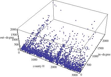
Figure 2: Joint plot of administrative county number and in- and out-degrees of the 3,107 counties, that is, the number of non-zero entries in rows and columns of the intercounty migration table. The ordering of counties is the same as in the first figure.

Figure 3: Joint plot of adminstrative county number and the 1995-2000 in-migrant and out-migrant totals for each of the 3,107 counties. The largest in-flows are to Los Angeles, California, Chicago [Cook County], Illinois and Houston [Harris County], Texas. The ordering of counties is the same as in the first two figures.

IV.3 First stage–bistochasticization of migration table

Counties vary widely in their number of in- and out-migrants (Fig. 3). To control for this (marginal/multiscale) effect, one may biproportionally/iteratively adjust the row and column sums (the ”Sinkhorn-Knopp algorithm” Knight (2008)) so that all $6,214=2\times 3,107$ such sums converge to be equal (say to 1). (This algorithm provides the basis of a measure–alternative to the PageRank employed by Google–of web page significance Knight (2008).) In Fig. 4, we show the $3,107\times 3,107$ intercounty migration table after such a bistochasticization (double-standardization).

Figure 4: Doubly-stochastic form of the 1995-2000 intercounty U. S. migration table. Fuzziness in Fig. 1 is greatly reduced. The correlation between the 735,531 non-zero entries of both these forms of the table is 0.15712, which can be increased to 0.27905 by taking the logs of the raw flows.

Clearly, the underlying definition/delimitation of blocks has been heightened by this transformation. The purpose of the scaling is to remove overall effects of size (which certainly may be of interest in themselves [Fig. 3]), and focus on the usually more intricate relative, interaction effects. Nevertheless, the cross-product ratios (relative odds), $\frac{m_{ij}m_{kl}}{m_{il}m_{kj}}$, measures of association, are left invariant in the process. Additionally, interestingly, the entries of the doubly-stochastic table provide maximum entropy estimates of the original flows, given the constraints on the row and column sums Eriksson (1980); Macgill (1977). So, this corresponds to an idealized situation in which all counties were constrained to emit and receive the same numbers of migrants.

IV.3.1 Eigenanalyses of bistochastic table

The dominant left and right eigenvectors (corresponding to the eigenvalue 1) of the doubly-standardized table are simply uniform vectors. The subdominant (left and right) eigenvectors (corresponding to a real eigenvalue of 0.90625) are of interest Meila and Pentney (2005). (The correlation between these two eigenvectors is high, 0.97119. The third largest eigenvalue is real also, 0.86878, while the fourth is slightly complex in nature, $0.84562+0.0009063i$. The vector of 3,107 eigenvalues has length 12.6472.) We reorder or seriate Fig. 4 on the basis of the left (in-migration) eigenvector and obtain Fig. 5, and on the basis of the right (out-migration) eigenvector and obtain Fig. 6. Now we see diminished clustering far from the diagonal. Further, both of these figures suggest the division of the nation into basically two large clusters.

IV.4 Second stage-strong component hierarchical clustering (SCHC)

Further, reordering on the basis of the (38-page-long, 3,107-county) dendrogram ((Slater, a, Supplement) epa ) generated by the strong component hierarchical clustering (the directed-graph analogue of the single-linkage method) Slater (1976a, 1984a, b, 1983b, 1984b, c, 1981); Tarjan (1982, 1983); Ozawa (1983) of the bistochasticized table, we obtain Fig. 7. The correlation between the ordering used in Fig. 7 and the admininstrative ordering used in Figs. 1 and 2 is 0.037352, and between the ordering used in Fig. 7 and the orderings used in Figs. 5 and 6, respectively, even lower, 0.004015 and 0.009995. (The corresponding correlations between the administrative ordering and the seriations employed in Figs. 5 and 6 are 0.057925 and 0.075508. Correlations greater in absolute value than 0.035307 are significant at the $95\%$ level, 0.040065 at the $97.5\%$ level, and 0.045826 at the $99\%$ level.)

IV.4.1 Cosmopolitan or hub-like behavior of counties

The dominant feature of Fig. 7 is that the counties now listed at the beginning in the reordering–and, in general, the last to be absorbed in the agglomerative clustering process–are “cosmopolitan” or “hub-like”. They tend to receive and send migrants across the nation, while those nearer to the end in the reordering tend to be more provincial or limited in their breadth of interactions Slater (1976b). (A prototypical example of a hub-like internal migration area is Paris Slater (1976b); Slater and Winchester (1978). In analytically parallel studies of interjournal citations Slater (1983b); Rosvall and Bergstrom (2008); Bollen et al. (2009), one might anticipate that the broad journals, Science, Nature and the Proceedings of the National Academy of Sciences might fulfill analogous roles.) This appears to be an interesting feature of the two-stage algorithm specific to it.

IV.4.2 Ultrametric (hierarchical) fit to the bistochastic and residuals therefrom

The ultrametric fit to this reordered bistochasticized table provided by the strong component hierarchical clustering Slater (1976a, 1984a, b, 1983b, 1984b, c, 1981); Tarjan (1982, 1983); Ozawa (1983) is given in Fig. 8, and the residuals (predominantly negative) from the hierarchical fit in Fig. 9. (These latter two figures, both in their own ways, further reflect this cosmopolitan-provincial dichotomy between the U. S. counties.) Let us also indicate that the two-stage methodology can be well-viewed well as BOTH a filtering AND coarse-graining procedure. This serves to cast light and understanding upon the predominantly largely negative residuals from the ultrametric fit to the doubly-stochastic table. (Usually, in fits of statistical models, one finds some rough balance between negative and positive residuals.)

IV.5 Possible effect of non-zero intracounty diagonal entries

Much earlier Slater (1983a, 1981) than this current paper, we had also studied (but without the aid of the more recently-developed computerized matrix plots used above) bistochasticized forms of the 1965-70 U. S. intercounty migration table with strong component hierarchical clustering Slater (1976a, 1984a, b, 1983b, 1984b, c, 1981); Tarjan (1982, 1983); Ozawa (1983), both with zero and non-zero (corresponding to intracounty movements) diagonal entries. Counties with large physical areas tend to absorb more of their own migrants, and thus exhibit larger diagonal bistochasticized entries and smaller off-diagonal entries in the non-zero-diagonal analysis, making them link at weaker levels in the dendrogram generated in the zero-diagonal analysis (cf. Montis et al. (2007)).

Journals with high self-citations would be expected to behave analogously in journal citation-matrix analyses Slater (1983b); Rosvall and Bergstrom (2008); Leydesdorff (2004). (In the application of our two-stage bistochasticization and strong component hierarchical clustering procedure to the 1967-75 interjournal citations between twenty-two mathematical journals, the Proceedings of the American Mathematical Society was found to function in a particularly broad, cosmopolitan manner in a zero-diagonal analysis Slater (1983b), while Advances in Mathematics played an analogous role when diagonal entries were taken into account.)

Figure 5: Doubly-stochastic matrix (Fig. 4) reordered on the basis of its subdominant left eigenvector. The first 72 counties in the ordering are all from Georgia (mostly lying in a [“Upper Coastal Plain”] band from the southwest corner of the state [Seminole County] to its north central boundary [Franklin, Hart, Elbert and Lincoln Counties]), and the last 110, all from the Great Plains states of North Dakota (45), South Dakota (50) and (north central) Nebraska (15). County 1000 is Bucks County, Pennsylvania and 2000, Lubbock County, Texas.

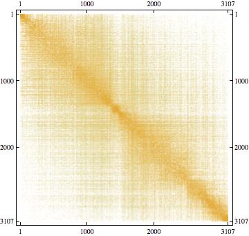
Figure 6: Doubly-stochastic matrix (Fig. 4) reordered on the basis of its subdominant right eigenvector. Rather similarly to Fig. 5, the first 74 counties in the ordering are all from Georgia, and the last 181, all from North Dakota, South Dakota, Nebraska and Minnesota. County 1000 is Washington County, Louisiana and 2000, Adair County, Oklahoma.

Figure 7: Doubly-stochastic matrix (Fig. 4) reordered on the basis of its strong component hierarchical clustering. The first twelve (“cosmopolitan”) counties in the seriation are all from the “Sunbelt” states of Florida (5 counties, a well-defined cluster of four of them being equivalent to the Tampa-St. Petersburg-Clearwater Metropolitan Statistical Area), Arizona (2), (southern) California (3), Nevada (Las Vegas) (1) and Texas (Dallas) (1). The last 35 (“provincial”) ones–lie principally in the “Black Belt”, stretching through the Deep South states of Mississippi (5), Alabama (24), Georgia (4) and (Panhandle) Florida (2). County 1000 is Carroll County, Indiana and 2000, Warren County, New Jersey.

Figure 8: Ultrametric (strong component hierarchical clustering [SCHC]) fit to the doubly-stochastic matrix Fig. 7. The fits tend to be higher in the lower right-hand corner, corresponding to the more “provincial” (including “Black Belt”) counties.

Figure 9: Residuals (predominantly negative) of the ultrametric fit (Fig. 8) to the doubly- stochastic matrix (Fig. 7). The residuals are most negative in the lower right-hand corner, where the fits provided by the strong component hierarchical clustering [SCHC] were greatest om value.

V Comparisons of bistochastic and disparity filters

In their response Serrano et al. (2009b) to the letter Slater (2009) commenting on their article Serrano et al. (2009a), Serrano, Boguñá and Vespignani (SBV) have called for ”an in-depth analysis of Slater’s [two-stage] technique on a set of standard multiscale networks and a thorough comparison of the results with respect to ours and other methods, as we have done in our paper [Serrano et al. (2009a)]”. Of course, this is a most appropriate proposal, which we now pursue in depth here.

The SBV methodology appears capable of producing a hierarchy of nodes, so direct comparisons in this regard should be possible Costa et al. (2006). Additionally, we can choose to take as an obvious candidate for the multiscale backbone, the 25,329 links required in our intercounty migration two-stage analysis above to complete the strong component hierarchical clustering (SCHC) Slater (a). (It would be of interest to overlay this backbone–both in raw and bistochastic form–on a county map of the United States [cf. (Slater, a, Figs. 1-4)]. If we, in a global filtering process, apply the SCHC to the largest raw migration flows, rather than to their bistochastic counterparts, it requires more than half-a-million, as opposed to 25,329 links, to complete the process.)

This can be compared with backbones generated by the techniques of SBV. (In (Radicchi et al., , p. 4), Radicchi, Ramasco and Fortunato wrote that the test of ”how many edges are needed to form a connected graph …has been suggested in” Serrano et al. (2009a). In an e-mail clarification of this point, Fortunato wrote ”What we referred to was Fig. 1 of the paper, in which they show how many nodes remain in the largest connected component after removing (or adding, if you wish) some fraction of the edges according to their method”.) Of course, by choosing thresholds one can truncate links in the SCHC backbone with smaller bistochastic values to include precisely any specific number of links one a priori desires in the backbone ultimately selected.

V.0.1 Correlations

Let us here note that the correlation between the 735,531 nonzero bistochastic values of the $3,107\times 3,107$ intercounty migration table and the corresponding signficance levels ($\alpha_{ij}$) of SBV is -0.33183, using an $OR$ rule, that is taking as the second variable $\mbox{Min}[\alpha_{ij}^{in},\alpha_{ij}^{out}]$ and -0.42094, with the use of an $AND$ rule, that is taking $\mbox{Max}[\alpha_{ij}^{in},\alpha_{ij}^{out}]$. Of course, we expect the correlations to be negative, since smaller $\alpha$’s indicate greater significance. We can strengthen the two correlations to -0.58630 and -0.64089, respectively, by using the logarithms of the bistochastic values, rather than the bistochastic values themselves.

The (notably strong) correlations between the logarithms of the 735,531 nonzero raw (unadjusted) flows and the corresponding values of $\mbox{Min}[\alpha_{ij}^{in},\alpha_{ij}^{out}]$ is -0.88681 and with $\mbox{Max}[\alpha_{ij}^{in},\alpha_{ij}^{out}]$, -0.84975. Thus, large raw flows certainly tend to be highly significant in the disparity filter model.

V.0.2 Cumulative plots

In the spirit of the analysis of SBV Serrano et al. (2009a), and in response to their call Serrano et al. (2009b) for further testing, we present Fig. 10. On the vertical axis–as a measure of total explanation–we plot the cumulative proportion (reaching 0.55029) of bistochastic flows (red curve) and the cumulative proportion (reaching 0.31626) of the corresponding raw (unadjusted) migration flows (blue) curve, as functions of the decreasingly ordered (from 1 to 0.022542) largest 25,329 links in the bistochastic table.

Let us note also that the correlation between the largest 25,329 bistochastic values and the correponding raw [flow] values is 0.045190, while the analogous correlation for the 735,531 non-zero raw and bistochastic flows is larger, 0.15712. These can be increased to 0.26249 and 0.27905, respectively, by using the logarithms of the raw flows, and further still to 0.31837 and 0.40843, respectively, by taking the logs of both the raw and bistochastic variables. Thus, large bistochastic values do exhibit a tendency to be associated with large raw values–but not as much as do the disparity filter significance levels.

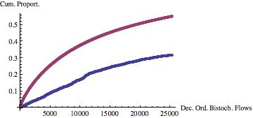
Figure 10: Cumulative proportions of decreasingly ordered bistochastic flows (higher red curve) and corresponding (non-ordered) raw flows (lower blue curve). The largest 25,329 bistochastic flows are needed to complete the strong component hierarchical clustering and can be considered to form the multiscale backbone of the network.

Further, in Fig. 11, we show the evolution of the SCHC agglomerative clustering process. As edges associated with smaller bistochastic values are introduced into the initially edge-less digraph, more previously isolated nodes are incorporated into nontrivial strong components, until with the 25,329th edge, associated with a bistochastic value of 0.022542 (for the flow from Indian River County, Florida to Brevard County, Florida), all 3,107 nodes (counties) are joined together to complete the clustering process (as well as forming a candidate for the multiscale backbone of the migration network).

Figure 11: Evolution of the strong component hierarchical clustering (SCHC) process. As edges with decreasing bistochstic values ($z$-axis) are introduced into the initially edge-less digraph, previously isolated nodes are incorporated into the multiscale backbone of the migration network, until eventually [with the 25,329th largest link] all nodes are joined together.

We have constructed a comparable figure to Fig. 11 based on the disparity filter of SBV (Serrano et al., 2009a, eq. (8), SI), using an $OR$ rule on the pair of in-flow and out-flow significance levels, $\alpha_{ij}^{in},\alpha_{ij}^{out}$. (We subtract the results from 1, in order to more directly graphically compare results based on the bistochastic values.) In Fig. 12, we show the evolution of the backbone as the significance level is raised.

Figure 12: Evolution of the disparity filter backbone of Serrano, Boguñá and Vespignani Serrano et al. (2009a), using $OR$ rule. As edges with decreasing values of $1-\mbox{Min}[\alpha_{ij}^{in},\alpha_{ij}^{out}]$ (plotted along the $z$-axis) are introduced into the initially edge-less digraph, previously isolated nodes are incorporated into nontrivial strong components forming the multiscale backbone of the migration network. For each of the 51,900 links employed, $\mbox{Min}[\alpha_{ij}^{in},\alpha_{ij}^{out}]<0.05$. The use of these links still leaves 15 individually isolated nodes (counties) (six neighboring ones from north central Nebraska), unincorporated into the backbone.

It would be of interest to jointly plot the data in Figs. 12 and 12 together with the plain link-weight threshold as were the figures in Serrano et al. (2009a).

V.0.3 Disparity filter–$OR$ rule with significance level $\alpha=0.01$

Employing the $OR$ rule on the migration links with a significance level of $\alpha=0.01$, the number of flows (edges) passing the test was 32,294 and the number of strong components in the associated candidate multiscale backbone was 67, with the backbone having $59.0179\%$ of the total edge weights (that is, the total number of migrants–47,240,477–recorded in the raw data table), a ”respectable” percentage. There was one giant component with 3,040 counties (cf. Dorogovtsev et al. (2001); Barbosa et al. (2003)), 65 isolated counties and one pair, Lipscomb and Ochiltree Counties, Texas (previously encountered with the two-stage algorithm). Again, the isolated (singleton) counties (none with in- or out-degree exceeding 115) were inland ones, not particularly notable as migration origins or destinations.

V.0.4 Disparity filter–$OR$ rule with significance levels $\alpha=0.14$ and $0.13$

With the $OR$ rule and a much weaker significance level, $\alpha=0.14$, there are 83,693 accepted edges, and all nodes do now lie in one strong component, and $73.0026\%$ of edge weights is included. (We note that $83,693>25,329$, the number of edges needed in the two-stage analysis Slater (a). For $\alpha=0.13$, there are 80,203 accepted edges and two strong components, with sparsely-populated [belittled?] King County, Texas, serving as a singleton.)

V.0.5 Disparity filter–$AND$ rule with significance level $\alpha=0.05$

The use of the disparity filter, using a significance level $\alpha=0.05$ on the $3,107\times 3,107$ raw migration table, together with an $AND$ rule (that is, a link must pass the significance test, viewed as both an inflow and an outflow) yielded 25,351 links–extremely close to the 25,329 links needed to complete the SCHC. However, with the slightly larger number of links obtained with the disparity filter, there were 181 distinct strong components (as opposed to only one with the application of the two-stage procedure). Of them, 174 were simply isolated nodes, and one ”giant” one consisting of 2,836 counties. This left six doublets (each pair comprised of contiguous counties): (1) the Georgia counties of Lincoln and Wilkes; (2) the Georgia counties of Stewart and Webster; (3) the California counties of Inyo and Mono; (4) the Nebraska counties of Nuckolls and Thayer; (5) the Kansas counties of Phillips and Smith; and (6) the Texas counties of Ochiltree and Lipscomb. (The greatest in- or out-degree–that is, the number of other counties to which migrants were sent or received–for any of these twelve counties was 146. With the exception of the first and fourth pairs listed, the same doublets were obtained in the two-stage analysis Slater (a).) All of the 174 isolated counties were located away from the Atlantic and Pacific coasts, with only one from Florida and none from California or Arizona. (The greatest in- or out-degree for any of these 174 counties was 132.) So, there does not seem to be any ”Sunbelt” or ”cosmopolitan” effect at work here.

V.0.6 Disparity filter–$AND$ rule with significance level $\alpha=0.001$

Using the $AND$ rule with $\alpha=0.001$, the resultant backbone has 10,153 links and 525 strong components, and $42.4254\%$ of the total edge weights. The largest component consists of 2,045 counties, while the next two largest are formed by 17 counties of the state of Montana, and 6 contiguous counties of eastern Nebraska. There are also two quintets (one comprised of Mississippi counties, and one of Kansas and Oklahoma counties) and four quartets (formed by Arkansas, Georgia, North Carolina and Texas counties).

VI Discussion of Related Issues

VI.1 Asymmetries

It would seem of interest and relevance to the study here of comparative properties of the two filtering procedures to also address a number of points raised in the response of SBV Serrano et al. (2009b) to the letter Slater (2009), commenting on their original (disparity filter) study Serrano et al. (2009a). SBV remark that the two-state algorithm can generate ”spurious asymmetries when the original network is symmetric.” (One can initiate the iterative proportional fitting [Sinkhorn-Knopp] procedure used to convert the flow matrix to bistochastic form by first normalizing rows or by first normalizing columns. However, this should not introduce significant asymmetries in the end result if suitable convergence is obtained.)

VI.2 Global/local issues

The use of ”globally” in the statement in Serrano et al. (2009b) that ”individual weights in the original matrix are globally normalized so that they can be compared on an equal footing” appears to suggest that the original flow matrix is simply scaled by a single number in the bistochastization–which is certainly not the case. (SBV assert that their methodology is more ”local” in nature than the two-stage procedure.) In this regard, let us observe that if one doubles, say, the entries in a single row or column of the flow matrix, then the results of both the two-stage algorithm and the disparity filter are completely invariant.

However, it is true that the decision whether or not to admit the $ij$-link into the network backbone depends only upon the entries in the $i$-th row and/or $j$-th column in the disparity filter, while this is certainly not the case with the bistochastic filter.

VI.3 Minimal spanning trees

In (Serrano et al., 2009a, p. 6484), SBV assert that ”reduced networks obtained [using the minimal spanning tree (MST)] are overly structural simplifications that destroy local cycles, clustering coefficient[s], and the clustering hierarchies often present in real world networks”. The MST is the basis for the method of single-linkage clustering. Further, the strong component hierarchical clustering (SCHC) procedure Tarjan (1983), we have widely applied (serving as the second-stage of the two-stage algorithm), can be viewed as the extension of single-linkage clustering to weighted, directed graphs. Therefore, the remark of SBV could be thought also to extend there. However, we think that this general criticism is quite easily and naturally addressed, if one supplements the specific links in the MST, using all those links having greater weight than the minimal one employed in the MST, rather than simply those links present in the MST. (If the insertion of a link does not succeed in joining hitherto disconnected components, it is not included in the MST, no matter how large its value. Tumminello et al have suggested extracting a subnetwork that can be embedded on a surface of genus $k$, rather than a tree Tumminello et al. (2005). Garas and Argyrakis study an ”Overlapping Tree Network”, which is based on the extraction of the MST, but allows for the filtered network to have loops Garas and Argyrakis (2009).)

One additional, interesting related observation to make is that with an undirected graph, and in the absence of links with precisely equal values, construction of the MST always unites just two connected components. In the strong component/directed graph analogue of the MST, the insertion of a new link can, in fact, even in the absence of links with identically equal values, join more than two strongly connected components.”

VI.4 Null models

SBV state that ”there is not a clear proposal for a suitable null model to measure the statistical significance of the results” [of the two-stage algorithm] Serrano et al. (2009b). (For corroboration, they refer to an early 1976 article Slater (1976a). However, later, in Slater (a), we did apply a graph-theoretic isolation criterion, we had also employed in 1981 and 1983, as well Slater (1983a, 1981), to rank clusters [regions] in terms of their statistical significance (cf. (Newman, 2003, sec. IV.3)).)

By way of illustration, in the 1965-70 US 3,140-county migration study, a statistical test of Ling Ling (1973) (designed for undirected graphs), based on the difference in the ranks of two edges, was employed in a heuristic manner (Slater, 1983a, pp. 7-8). For example, the 3,148th largest doubly-stochastic value, 0.12972 (corresponding to the flow from Maui County to Hawaii County), united the four counties of the state of Hawaii. The (considerably weaker) 7,939th largest value, 0.07340 (the link from Kauai County, Hawaii, to Nome, Alaska), integrated the four-county state of Hawaii into a much larger 2,464-county cluster. The difference of these two ranks, 4,192 = 7,340 - 3,148, is a measure of isolation (“survival time”) of this state as a cluster. Reference to Table 1 in Slater (1983a) showed the significance of the state of Hawaii as a functional internal migration unit at the 0.01 level (Slater, 1983a, p. 7). (In the computation of this table, the approximation was used that the number of edges in the relevant digraphs was a negligible proportion of all possible $3,140\times 3,139$ edges.)

In these regards, it would also seem natural to investigate exploiting the notion of a ”random doubly-stochastic matrix” Griffiths (1974); Życzkowski et al. (2003). (Potentially useful then would be the seminal result of Birkhoff that any $n\times n$ doubly-stochastic matrix can be written as a convex combination of at most $n^{2}$ permutation matrices–those with a single 1 in each row and column, and zeros elsewhere.)

VI.5 Properties of bistochastic matrices

Let us further make the general observations that powers of bistochastic matrices are also bistochastic. Higher-order powers (in line with properties of Markov chains and the famous Perron-Frobenius Theorem), are smoother and more uniform in nature, while in the infinite limit, convergence to an $n\times n$ table with all entries equal to $\frac{1}{n}$ is attained. (This might be viewed as an interesting manifestation of all nodes being treated equally, that is, not belittled.) Mathematical physicists have been interested in developing conditions that indicate when a bistochastic matrix is also unistochastic Louck (1997); Życzkowski et al. (2003); Bengtsson et al. (2005); Diţă (2006). (This is the case if the $ij$-bistochastic entry is the square of the absolute value of the $ij$-entry of a unitary matrix.) It would be interesting to investigate whether or not unistochasticity is of value in the modeling of network flows.) An efficient algorithm–considered as a nonlinear dynamical system–to generate random bistochastic matrices has recently been presented Cappellini et al. (cf. Griffiths (1974); Życzkowski et al. (2003)). (Gudder has quite recently developed the concept of a bistochastic transition effect matrix Gudder (2009).)

VI.6 Cosmopolitan/provincial dichotomy

Although, by no means, have we yet systematically compared the clustering structures produced by the bistochastic and disparity filter approaches in our 1995-2000 migration analysis, the two methods–as noted in our preceding discussions–do seem to yield rather different (but still largely contiguous) results (regions). One distinguishing, highly attractive feature of the bistochastic approach has been its ability to contrast ”cosmopolitan” (hub-like or centralized) units from ”provincial/local” ones. We are not aware of any comparable feature with the disparity filter.

Geographic subdivisions (or groups of subdivisions) that enter into the bulk of the dendrograms produced by the two-stage procedure at the weakest levels are those with the broadest ties. These are “cosmopolitan”, hub-like areas, a prototypical example being the French capital, Paris (Slater, 1984a, Sec. 4.1) Slater (1976b). Similarly, in parallel analyses of other internal migration tables, the cosmopolitan/non-provincial natures of London Slater (1978), Barcelona Slater (1976d) (Slater, 1984a, Sec. 6.2, Figs. 36, 37), Milan Gentileschi and Slater (1980) (Slater, 1984a, Sec. 6.3, Figs. 39, 40) (cf. Slater (1975c)), Amsterdam (Slater, 1984a, p. 78) Masser and Scheurwater (1980), West Berlin (Slater, 1984a, p. 80), Moscow (the city and the oblast as a unit) Slater (1975a) (Slater, 1984a, Sec. 5.1 and Figs. 6, 7), Manila (coupled with suburban Rizal) Slater (1982), Bucharest Slater (1979), Île-de-Montréal (Slater, 1984a, p. 87), Zürich, Santiago, Tunis and Istanbul Slater (1975b) were–among others–highlighted in the respective dendrograms for their nations (Slater, 1984a, Sec. 8.2) (Slater, 1981, pp. 181-182) (Slater, 1983b, p. 55).

In our previous 1965-70 intercounty analysis for the US, the most cosmopolitan entities were: (1) the centrally-located paired Illinois counties of Cook (Chicago) and neighboring, suburban DuPage; (2) the nation’s capital, Washington, D. C.; and (3) the paired South Florida (retirement) counties of Dade (Miami) and Broward (Ft. Lauderdale) Slater (1983a, 1984b, 1984c). In general, counties with large military installations, large college populations or state capitals also interacted broadly with other areas (Slater, 1983a, p. 153). Application of the two-stage methodology to 1965-66 London inter-borough migration Masser and Scheurwater (1980) indicated that the three inner boroughs of Kensington and Chelsea, Westminster, and Hammersmith acted–as a unit–in a cosmopolitan manner (Slater, 1984a, Sec. 5.2, Fig. 10). (In Sec. 8.2 and Table 16 of the anthology of results Slater (1984a), additional geographic units and groups of units found to be cosmopolitan with regard to migration, are enumerated.)

VI.7 Clusters/regions obtained in two-stage internal migration analyses

Geographically isolated (insular) areas–such as the Japanese islands of Kyushu and Shikoku Slater (1976a)–emerged as well-defined clusters (regions) of their constituent (seven and four, respectively) subdivisions (“prefectures” in the Japanese case) in the dendrograms for the corresponding two-stage analyses, and similarly the Italian islands of Sicily and Sardinia Gentileschi and Slater (1980), the North and South Islands of New Zealand, and the Canadian islands of Newfoundland and Prince Edward Island (Slater, 1984a, p. 90) (cf. E et al. (2008); Slater (1976e)). The eight counties of Connecticut, and other New England groupings, as further examples, to be elaborated upon below, were also very prominent in the highly disaggregated U. S. analysis Slater (1983a). Relatedly, in a study based solely upon the 1968 movement of college students among the fifty states, the six New England states were strongly clustered (Slater, 1976f, Fig. 1). Employing a 1963 Spanish interprovincial migration table, well-defined regions were formed by the two provinces of the Canary Islands, and the four provinces of Galicia Slater (1976d) (Slater, 1984a, Sec. 6.2.1, Fig. 37) (cf. Slater (1976e)). The southernmost Indian states of Kerala and Madras (now Tamil Nadu) were strongly paired on the basis of 1961 interstate flows Slater (1976g).

A detailed comparison between functional migration regions found by the two-stage procedure and those actually employed for administrative, political purposes in the corresponding nations is given in Sec. 8.1 and Table 15 of Slater (1984a). (In the 1995-2000 U. S. analysis at hand, particularly distinct large multicounty migration regions, well describable as ”French Louisiana”, ”Northern Lower Michigan”, ”Northern New England”, ”South Jersey”… were found (Slater, a, Tables I, II).)

VI.7.1 Rarity of noncontiguous groupings

In a 1989 monograph, Gawryszewski Gawryszewski (1989, 1992) attempts to regionalize–presenting numerous dendrograms–the voivodships (provinces) of Poland on the basis of (total, rural-to-urban, and urban-to-urban) internal migration in the 1952-83 period, using the two-stage algorithm.

It should be noted that it is rare that the two-stage methodology yields a migration region composed of two or more noncontiguous subregions–even though no contiguity information, of course, is explicitly present in the flow table nor provided to the algorithm (cf. Lin and Xie (1998); Slater (1980)). A notable exception–comprehensible in terms of regional disparities in wealth, however–to this (topological) rule was the uniting of the northern Italian region of Piemonte–the location of industrial Turin, where Fiat is based–with (poor) southern regions, before joining with central regions, in an aggregate 18-region 1955-70 study Slater (1975c) (Slater, 1984a, p. 75) (cf. Gentileschi and Slater (1980) and (Slater, a, p. 26)) .

VII Concluding remarks

The observation that far fewer links (25,329 vs. more than 80,203 (cf. [Fig. 12])) are needed to construct a strongly connected network backbone in the bistochastic case Slater (a) than in the disparity analysis, appears, for the specific dataset at hand, to serve as a positive aspect of the bistochastic filtering methodology. Another positive feature is the fact that the correlations of the logarithms of the 735,531 nonzero raw (unadjusted) intercounty migration flows with the logs of the corresponding bistochasticized links is 0.318379, but with the disparity filter significance levels, considerably stronger in nature, that is, -0.849757 (using the $AND$ rule) and -0.886816 ($OR$ rule). Thus, in terms of the criteria put forth by Serrano, Boguñá and Vespignani themselves Serrano et al. (2009a), it appears that the bistochastic filter, desirably, ”belittles” small flows (and nodes) less so than does the SBV disparity filter.

Nevertheless,more detailed comparative studies, in particular as to ”topological” properties, as called for by SBV, are certainly in order. (One important topological property is that of strong connectedness, upon which the second stage of the two-stage algorithm Slater (1984a) is based. Another is the pronounced rarity–even in the absence of imposition of contiguity constraints–of noncontiguous couplings observed [sec. VI.7] in the numerous two-stage internal migration analyses of various nations that have been conducted. This phenomenon is well exhibited in the 3,000+ U. S. county dendrogram in the supplementary material, and would be immediately apparent in the correspondingly reordered doubly-stochastic internal migration matrix (Fig. 7) if county-state labels could be attached to the rows and columns.)

VII.1 Gedanken experiment

Somewhat contrastingly, one might consider a gedanken experiment, in which a (”non-multiscale”) network in precisely bistochastic (or proportional thereto) form is empirically (and remarkably!) obtained. Then, bistochastic filtering would not alter the internodal scores in any manner, while presumably disparity filtering would. Clearly, the correlation between the filtered and raw scores would be perfect (1.0) in the bistochastic scenario and weaker (in contrast to our main U. S. intercounty migration analysis above) with the disparity filter.

VII.2 Domains of applicability

Finally, let us remark that the two methodologies would seem to work better in different domains: the disparity filtering approach of SBV may be more appropriate when small samples are involved and the use of measures of significance of flows are indicated, while the two-stage methodology employs (bistochastic) measures of association, and perhaps is more effective in constructing a network backbone when considerable data are at hand. This is an analytical dichotomy–that of finding a suitable balance between significance and sample size–which had already arisen several decades ago in the influential ”transaction flow” models of Savage, and Deutsch and Brams Savage and Deutsch (1960); Brams (1966) in the political science literature (cf. Mosteller (1968)).