Properties of dusty tori in active galactic nuclei - II. Type 2 AGN

Abstract

This paper is the second part of a work investigating the properties of dusty tori in active galactic nuclei (AGN) by means of multi-component spectral energy distribution (SED) fitting. It focuses on low luminosity, low redshift ($z\leq 0.25$) AGN selected among emission line galaxies in the overlapping regions between SWIRE and SDSS Data Release 4 as well as X-ray, radio and mid-infrared selected type 2 AGN samples from the literature. The available multi-band photometry covers the spectral range from the $u$-band up to 160µm. Using a standard $\chi^{2}$ minimisation, the observed SED of each object is fit to a set of multi-component models comprising a stellar component, a high optical depth ($\tau_{9.7}\geq 1.0$) torus and cold emission from a starburst (SB). The torus components assigned to the majority of the objects were those of the highest optical depth of our grid of models ($\tau_{9.7}=10.0$). The contribution of the various components (stars, torus, SB) is reflected in the position of the objects on the IRAC colour diagram, with star-, torus- and starburst-dominated objects occupying specific areas of the diagrams and composite objects lying in between. The comparison of type 1 (as derived from Paper 1, Hatziminaoglou et al. 2008) and type 2 AGN properties is broadly consistent with the Unified Scheme. The estimated ratio between type 2 and type 1 objects is about 2-2.5:1. The AGN accretion-to-infrared luminosity ratio is an indicator of the obscuration of the AGN since it scales down with the covering factor. We find evidence supporting the receding torus paradigm, with the estimated fraction of obscured AGN, derived from the distribution of the covering factor, decreasing with increasing optical luminosity ($\lambda L_{5100}$) over four orders of magnitude. The average star formation rates are of $\sim 10M_{\odot}/yr$ for the low-$z$ sample, $\sim 40M_{\odot}/yr$ for the other type 2 AGN and $\sim 115M_{\odot}/yr$ for the quasars; this result however, might simply reflect observational biases, as the quasars under study were one to two orders of magnitude more luminous than the various type 2 AGN. For the large majority of objects with 70 and/or 160 µm detections an SB component was needed in order to reproduce the data points, implying that the far-infrared emission in AGN arises mostly from star formation; moreover, the starburst-to-AGN luminosity ratio shows a slight trend with increasing luminosity.

1 INTRODUCTION

Dust is the cornerstone of the active galactic nuclei (AGN) Unified Scheme that postulates that the diversity of the observed properties of AGN are merely a result of the different lines of sight with respect to obscuring material surrounding the active nucleus (Antonucci 1993; Urri & Padovani 1995; Tadhunter 2008). The elements necessary for understanding the nature of AGN and the variety of their properties are in fact the geometry of the circumnuclear dust and the amount of obscuration. The latter is also needed in order to understand the physical conditions of the dust enshrouded nuclear region and to estimate the intrinsic UV-to-optical properties of the AGN. Obscuring dusty material should re-radiate in the infrared (IR) the fraction of accretion luminosity it absorbs, providing thus a direct metric for the study of the medium. Indeed all spectroscopically confirmed AGN lying in regions covered by the various Spitzer Space Telescope (Spitzer) surveys show significant IR emission down to the detection limits.

The conventional wisdom is that dust, distributed in a more or less toroidal form around the nucleus, mainly consists of silicate and graphite grains, leaving unmistakable signatures in the observed SEDs of AGN. The most important dust features are the T$\simeq$1500 black-body like rise of the IR emission at $\lambda\geq 1$ µm, corresponding to the sublimation temperature of the graphite grains and the $\sim$9.7 micron feature in emission/absorption attributed to silicates. While silicates in absorption were already long ago observed in a variety of type 2 objects, ISO observations only provided faint indications of their presence in emission in the spectra of type 1, challenging the Unified Scheme, as all smooth torus models predicted a feature in emission for the unobscured AGN. Clumpy models, on the other hand, provided a natural attenuation of the feature (Nenkova et al., 2002). Observations of tens of objects carried out with the IRS spectrograph onboard Spitzer allowed, however, the detection of the silicate feature (first reported by Siebenmorgen et al. 2005 and observed by several others since) predicted by smooth tori models in emission for type 1 AGN and quasars (e.g. Pier & Krolik 1992; Granato & Danese 1994; Fritz et al. 2006). Thus far, there is no consensus on the dust distribution among astronomers; for an overview of the issues involving the two approaches see Dullemond & van Bemmel (2005), Elitzur (2008) and Nenkova et al. (2008).

Until very recently the number of spectroscopically confirmed type 2 AGN was rather limited; in the last few years however, the advent of large-scale multi-wavelength surveys has led to a revolution in AGN studies. We are now in a position to compile statistically large type 2 AGN samples at all redshifts, selected in a multitude of ways. In this work we try to characterise the observed spectral energy distribution (SED) of type 2 AGN using the smooth torus models described in Fritz et al. (2006) and the methodology described in Hatziminaoglou et al. (2008), hereafter Paper 1, in which we dealt with the IR properties of quasars. The aim of the present work is to model a large sample of type 2 AGN and, by comparison with the results derived from the study of type 1 quasars in Paper 1, test the Unified Scheme. The various type 2 AGN samples will be discussed in detail in Section 2. Section 3 will briefly describe the various model components as well as the basics of the standard $\chi^{2}$ minimisation technique and assumptions. The results on the individual samples will be presented in Section 4 while the combined results from all samples, including the quasars (typical representatives of type 1 AGN) from Paper 1, will be shown in Section 5. A final discussion on the future of such studies is presented in Section 6.

2 THE SAMPLES

In this work we will be analysing a variety of type 2 AGN samples, namely a low redshift, low luminosity AGN sample, an X-ray and radio selected sample in the COSMOS field and a mid-infrared (MIR) selected sample from the ELAIS fields. We will be also revisiting the SDSS/SWIRE quasar sample studied in Paper 1 (hereafter quasar sample).

2.1 Low-luminosity low-redshift AGN

The low-luminosity low-redshift AGN sample, hereafter low-$z$ sample, is part of an updated version of an emission line galaxies sample classified as AGN. The selection was made among hundreds of thousands of emission line galaxies from the SDSS Data Release 4 (DR4; Adelman-McCarthy et al. 2006), based on the relative strength of the emission lines on a log([Oiii]/H$\beta$) - log([Nii]/H$\alpha$) diagram, after careful subtraction of the stellar continuum, described in detail on Kauffmann et al. (2003) . From the more than 80,000 proposed AGN, 420 reside in the northern SWIRE (Lonsdale et al. 2003; Lonsdale et al. 2004) fields ELAIS N1, ELAIS N2 and Lockman. Among these objects, 388 have been detected in at least two out of the four IRAC bands, with 340 having also MIPS detections at 24 µm. From the 388 (340 with an additional 24 µm detection) objects, 155 (146) and 88 (81) were additionally detected by MIPS at 70 and 160 µm, respectively. The far-infrared (FIR) measurements characterize or constrain (with upper limits) the cold dust emission.

Due to the nature of the sample, particular care was taken in the construction of the SEDs. We used data from the SDSS DR4, 2MASS including the deeper data set 2MASS $\times$ 6 taken in the Lockman field (Beichman et al., 2003), as well as IR data from SWIRE. For extended objects (based on the SDSS classification) we used Petrosian $u$, $g$, $r$, $i$, $z$ magnitudes, 7” radius magnitudes for 2MASS $JHK$, and aperture 5 fluxes (5.8” radius), the largest publicly available IRAC aperture, for the four IRAC bands, to better capture the total light arising from the resolved host galaxies. The 5” 2MASS magnitudes, closer to the 5.8” aperture selected for the IRAC bands, were proven to be inadequate when all the SEDs were visually inspected as they were clearly falling short of both the SDSS and the IRAC fluxes. For the point sources we used PSF SDSS magnitudes, default (PSF) 2MASS magnitudes and aperture 2 (1.9”) IRAC magnitudes (for a full description of the SWIRE magnitudes and their adequate for point-like and extended sources see Surace et al. 2005). The redshift histogram of the 420 objects is shown in Fig. 1, with the gray histogram corresponding to the 388 objects that will be studied in detail. Tables 1 and 2 show the SDSS names, coordinates, redshifts, emission line properties, and stellar masses (taken from the narrow emission line object catalogue), and SWIRE fluxes, respectively for the 420 objects. The objects belonging to the Subset (S) of 388 entries used for the study are marked in the column “S” of Table 1. The objects marked in column “AGN” are those that were assigned with an AGN component as a result of the fitting procedure.

Table 1: SDSS names, coordinates, redshifts, emission line properties, and stellar masses for the 420 objects overlapping the SWIRE fields and the narrow emission line object catalogue from Kauffmann et al (2003). Column called “S” (for Subset) marks the objects that have an adequate sampling of their SEDs and will be used in the analysis. The full catalogue is available online.

SqNr	S	SDSS name	RA	Dec	$z$	log[OIII]	log[OIII/Hb]	log[NII/Ha]	logM∗[M⊙]
1		SDSS_J160215.17+535456.1	16:02:15.17	+53:54:56.1	0.081	6.2711	0.341	-0.0537	11.065
2	X	SDSS_J160258.45+540929.1	16:02:58.45	+54:09:29.1	0.065	5.6622	0.113	0.1397	10.4765
3	X	SDSS_J160300.04+541737.3	16:03:00.04	+54:17:37.3	0.106	5.862	0.0946	-0.0224	11.1844
4	X	SDSS_J160221.35+541105.0	16:02:21.35	+54:11:05.0	0.066	6.4168	-0.0782	-0.2444	11.2855
5		SDSS_J160006.83+541717.2	16:00:06.83	+54:17:17.2	0.066	6.4527	-0.115	-0.2069	10.5041
6	X	SDSS_J160114.70+542034.3	16:01:14.70	+54:20:34.3	0.064	7.7295	-0.1227	-0.2971	10.7284
7	X	SDSS_J160035.48+541529.2	16:00:35.48	+54:15:29.2	0.064	6.1645	0.4281	-0.1508	10.7402
8		SDSS_J155713.43+543953.9	15:57:13.43	+54:39:53.9	0.045	5.9737	-0.0429	-0.0453	10.712
9	X	SDSS_J155813.02+543656.1	15:58:13.02	+54:36:56.1	0.047	5.6459	-0.2685	-0.2906	10.4376
10		SDSS_J155705.98+543902.0	15:57:05.98	+54:39:02.0	0.045	6.261	-0.0665	0.0228	10.8279
11		SDSS_J155708.97+544355.7	15:57:08.97	+54:43:55.7	0.047	5.6832	0.1481	0.0986	10.7445
12	X	SDSS_J160007.28+545350.0	16:00:07.28	+54:53:50.0	0.084	7.264	-0.3575	-0.247	10.5545
13	X	SDSS_J155940.66+545050.8	15:59:40.66	+54:50:50.8	0.093	6.031	0.2662	0.0451	10.9104
14	X	SDSS_J160218.41+544718.5	16:02:18.41	+54:47:18.5	0.083	6.887	0.0743	-0.1568	10.6365
15	X	SDSS_J160254.28+545540.7	16:02:54.28	+54:55:40.7	0.120	6.5346	0.3394	0.1132	11.1944
16	X	SDSS_J160124.58+550120.1	16:01:24.58	+55:01:20.1	0.037	7.1557	0.7	0.0261	10.6611
17	X	SDSS_J160512.63+545550.7	16:05:12.63	+54:55:50.7	0.064	6.0292	0.7485	-0.0783	9.9791
18	X	SDSS_J160122.30+552213.6	16:01:22.30	+55:22:13.6	0.119	6.3901	-0.3305	-0.1667	10.9273
19		SDSS_J161320.00+525516.4	16:13:20.00	+52:55:16.4	0.166	8.0556	0.3297	-0.1401	11.2084
20	X	SDSS_J161339.10+531833.6	16:13:39.10	+53:18:33.6	0.107	7.3537	-0.2625	-0.2766	11.1697

Table 2: SWIRE fluxes of the sample presented in Table 1. The typical errors on the 70 and 160 µm fluxes are 10% of the fluxes. The column “AGN” denotes the objects that, after the fitting, were found to have an AGN component and on which all AGN-related analysis is based. The full sample is available online.

SqNr	S3.6 [$\mu$Jy]	S4.5 [$\mu$Jy]	S5.8 [$\mu$Jy]	S8.0 [$\mu$Jy]	S24 [$\mu$Jy]	S70 [$\mu$Jy]	S160 [$\mu$Jy]	AGN
1					649.83 $\pm$ 25.48
2	982.65 $\pm$ 4.09	642.35 $\pm$ 3.17	463.57 $\pm$ 9.7	786.24 $\pm$ 8.26	522.05 $\pm$ 12.92
3	1601.7 $\pm$ 4.57	1112.9 $\pm$ 4.39	760.76 $\pm$ 10.71	602.03 $\pm$ 5.61
4	4056.2 $\pm$ 13.12	2806.7 $\pm$ 6.52	2756.1 $\pm$ 21.18	8360.2 $\pm$ 14.44	7091.1 $\pm$ 21.25	115570.0	574590.0
5					4851.0 $\pm$ 21.13	15020.0
6	1707.0 $\pm$ 6.56	1213.2 $\pm$ 3.69	1483.1 $\pm$ 17.45	5734.6 $\pm$ 11.03	9659.0 $\pm$ 21.62	129220.0	218440.0
7		1119.1 $\pm$ 7.12		514.31 $\pm$ 14.09	407.65 $\pm$ 16.67
8					1964.0 $\pm$ 14.73
9		826.02 $\pm$ 4.27		760.54 $\pm$ 12.53	1099.9 $\pm$ 16.91
10					5237.6 $\pm$ 20.65	92560.0	360010.0
11					480.31 $\pm$ 15.1
12	1321.2 $\pm$ 2.47	924.4 $\pm$ 2.53	925.13 $\pm$ 7.79	4547.6 $\pm$ 8.6	5377.6 $\pm$ 20.53	67840.0	80250.0
13	1202.8 $\pm$ 2.89	825.9 $\pm$ 3.01	515.12 $\pm$ 9.01	699.14 $\pm$ 8.67	169.76 $\pm$ 17.27
14	1134.7 $\pm$ 2.58	751.64 $\pm$ 2.74	559.29 $\pm$ 6.58	1201.9 $\pm$ 7.39	932.88 $\pm$ 17.15
15	1379.4 $\pm$ 3.89	1008.8 $\pm$ 4.39	698.5 $\pm$ 8.38	1753.8 $\pm$ 8.52	2398.5 $\pm$ 16.42	1620.0
16	2722.7 $\pm$ 3.44	1720.6 $\pm$ 3.18	1365.3 $\pm$ 8.46	1661.1 $\pm$ 7.45	1232.4 $\pm$ 13.53
17	512.8 $\pm$ 2.4	318.82 $\pm$ 2.88	231.09 $\pm$ 7.23	182.6 $\pm$ 8.5	171.23 $\pm$ 16.42
18	929.66 $\pm$ 2.98	681.77 $\pm$ 3.56	502.83 $\pm$ 8.02	1214.6 $\pm$ 9.39	1153.0 $\pm$ 17.27	6960.0	2010.0	X
19					2803.6 $\pm$ 19.2	32840.0
20	1653.2 $\pm$ 2.66	1281.6 $\pm$ 3.46	1343.0 $\pm$ 8.09	8447.7 $\pm$ 12.28	9574.3 $\pm$ 22.22	131310.0	396400.0

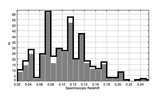
Figure 1: Redshift histogram of the low luminosity low redshift AGN sample selected from Kauffmann et al. 2003. The grey shading indicates sources with good photometric coverage allowing detailed study.

2.2 X-ray, radio and Mid-IR selected type 2 AGN

The next sample, hereafter COSMOS sample, consists of AGN selected among X-ray and radio emitters in the COSMOS field (Trump et al., 2007). Among the 466 objects for which Magellan spectroscopy was carried out, were 135 type 2 AGN and hybrids (type 2s with a galaxy component; for details on the classification see Trump et al. 2007) with optical and IRAC counterparts. For the optical/near-IR photometry we used the COSMOS first release optical and near-IR catalogue Capak et al. (2007). The IRAC and MIPS photometry was taken from the S-COSMOS May 2007 release, described in Sanders et al. 2007. From the 135 objects, 92 have a 24 micron counterpart and they alone will be the objects to be studied, as will be discussed in Section 4.2.

To construct the SED of these 92 objects we used the $u^{*}$- and $i^{*}$-band CFHT data, the $g^{+}$, $V_{j}$, $r^{+}$, and $z^{+}$ Subaru data, the $K_{S}$ KPNO or CTIO data and the IRAC and MIPS S-COSMOS data. Photometry from the MIPS 24µm deep scans was used whenever available. The $B_{j}$ band data were discarded due to the large overlap with $g^{+}$-band that would lead to overly redundant information and the CFHT $i^{*}$ was used instead of the Subaru $i^{+}$ because some of the objects were missing from the Subaru $i^{+}$-band data (even though, according to Capak et al. 2007 the latter observations are deeper by two magnitudes). Tables 3 and 4 show the COSMOS names, coordinates, redshifts and type (“q2” for type 2 AGN, “q2e” for hybrid and a question mark next to the type denotes a questionable classification) taken from Trump et al. (2007), Table 2, and the Spitzer fluxes (from Sanders et al. 2007), respectively, for the first 20 objects of the sample. The full tables are available online.

Table 3: COSMOS names, coordinates, redshifts and classification type for the COSMOS type 2 AGN sample, from Trump et al. 2007. The full catalogue is available online.

SqNr	COSMOS Names	RA	Dec	$z$	Type
1	COSMOS_J100033.08+015414.4	10:00:33.08	+01:54:14.4	1.16908	q2?
2	COSMOS_J095945.18+023439.4	09:59:45.18	+02:34:39.4	0.47717	q2e
3	COSMOS_J095943.76+022008.0	09:59:43.76	+02:20:08.0	0.92998	q2e
4	COSMOS_J100035.25+015726.0	10:00:35.25	+01:57:26.0	0.84845	q2e
5	COSMOS_J100059.47+022631.8	10:00:59.47	+02:26:31.8	0.66944	q2e
6	COSMOS_J100204.84+013356.0	10:02:04.84	+01:33:56.0	0.09815	q2
7	COSMOS_J100013.73+021221.3	10:00:13.73	+02:12:21.3	0.18645	q2
8	COSMOS_J095933.79+014906.3	09:59:33.79	+01:49:06.3	0.13327	q2
9	COSMOS_J100028.69+021745.3	10:00:28.69	+02:17:45.3	1.03911	q2?
10	COSMOS_J100107.22+020115.8	10:01:07.22	+02:01:15.8	0.24672	q2
11	COSMOS_J100223.62+021132.8	10:02:23.62	+02:11:32.8	0.12262	q2e
12	COSMOS_J100211.38+015633.2	10:02:11.37	+01:56:33.2	0.21752	q2
13	COSMOS_J100243.25+020521.9	10:02:43.25	+02:05:21.9	0.21398	q2
14	COSMOS_J100022.94+021312.7	10:00:22.94	+02:13:12.7	0.18583	q2
15	COSMOS_J100135.22+023109.1	10:01:35.23	+02:31:09.1	0.21898	q2
16	COSMOS_J095934.89+015241.1	09:59:34.89	+01:52:41.1	0.13333	q2
17	COSMOS_J100152.90+020113.7	10:01:52.90	+02:01:13.7	0.22042	q2
18	COSMOS_J100118.97+020822.5	10:01:18.97	+02:08:22.5	0.16768	q2
19	COSMOS_J100231.87+015926.7	10:02:31.87	+01:59:26.7	0.80314	q2
20	COSMOS_J095945.18+015330.4	09:59:45.18	+01:53:30.4	0.21987	q2e

Table 4: COSMOS Spitzer fluxes of the sample presented in Table 3. The errors on the 70 and 160 µm fluxes are 10% of the fluxes. The full sample is available online.

SqNr	S3.6 [$\mu$Jy]	S4.5 [$\mu$Jy]	S5.8 [$\mu$Jy]	S8.0 [$\mu$Jy]	S24 [$\mu$Jy]	S70 [$\mu$Jy]	S160 [$\mu$Jy]
1	148.19 $\pm$ 0.26	145.3 $\pm$ 0.27	108.12 $\pm$ 0.74	680.25 $\pm$ 1.55	2819.9 $\pm$ 115.8	48550.0
2	329.74 $\pm$ 0.4	239.16 $\pm$ 0.42	155.24 $\pm$ 0.74	302.6 $\pm$ 1.77	502.5 $\pm$ 11.5
3	116.34 $\pm$ 0.23	102.27 $\pm$ 0.26	96.91 $\pm$ 0.77	125.99 $\pm$ 1.47	562.8 $\pm$ 10.8
4	108.87 $\pm$ 0.22	114.63 $\pm$ 0.27	75.65 $\pm$ 0.74	235.19 $\pm$ 1.52	687.8 $\pm$ 111.5
5	10.37 $\pm$ 0.1	18.13 $\pm$ 0.17	34.93 $\pm$ 0.61	92.23 $\pm$ 1.3	851.0 $\pm$ 108.2
6	806.09 $\pm$ 0.89	627.66 $\pm$ 0.7	767.83 $\pm$ 1.38	5846.26 $\pm$ 4.76	8750.9 $\pm$ 170.7	187800.0
7	132.39 $\pm$ 0.2	106.82 $\pm$ 0.25	71.29 $\pm$ 0.62	262.16 $\pm$ 1.44	3295.0 $\pm$ 42.3
8	376.01 $\pm$ 0.45	279.86 $\pm$ 0.39	267.35 $\pm$ 0.84	2175.11 $\pm$ 2.45	3684.0 $\pm$ 115.0	73760.0	219900.0
9	33.02 $\pm$ 0.14	41.25 $\pm$ 0.2	43.11 $\pm$ 0.72	44.6 $\pm$ 1.41	396.7 $\pm$ 112.0
10	73.22 $\pm$ 0.17	80.59 $\pm$ 0.24	56.14 $\pm$ 0.67	300.27 $\pm$ 1.58	517.2 $\pm$ 96.7
11	365.01 $\pm$ 0.4	285.97 $\pm$ 0.38	255.93 $\pm$ 0.77	1464.55 $\pm$ 1.97	1957.6 $\pm$ 108.3	55820.0
12	80.37 $\pm$ 0.17	75.51 $\pm$ 0.21	48.93 $\pm$ 0.61	292.38 $\pm$ 1.39	654.9 $\pm$ 112.3
13	242.32 $\pm$ 0.33	228.27 $\pm$ 0.31	172.33 $\pm$ 0.78	1058.68 $\pm$ 1.69	2214.2 $\pm$ 94.0
14	246.44 $\pm$ 0.31	203.64 $\pm$ 0.33	159.9 $\pm$ 0.73	1273.79 $\pm$ 2.03	6399.4 $\pm$ 111.3	63680.0
15	90.39 $\pm$ 0.19	84.12 $\pm$ 0.22	57.78 $\pm$ 0.68	373.63 $\pm$ 1.48	1189.4 $\pm$ 222.1
16	196.56 $\pm$ 0.27	164.13 $\pm$ 0.3	136.25 $\pm$ 0.67	489.73 $\pm$ 1.55	1886.0 $\pm$ 108.8
17	118.25 $\pm$ 0.23	114.71 $\pm$ 0.27	73.56 $\pm$ 0.71	454.65 $\pm$ 1.62	1164.5 $\pm$ 111.0
18	285.06 $\pm$ 0.4	231.32 $\pm$ 0.36	178.53 $\pm$ 0.84	1378.11 $\pm$ 2.13	2221.6 $\pm$ 109.6	42480.0
19	22.08 $\pm$ 0.12	19.33 $\pm$ 0.18	18.82 $\pm$ 0.59	38.77 $\pm$ 1.34	1843.1 $\pm$ 94.6
20	81.2 $\pm$ 0.17	72.98 $\pm$ 0.2	42.49 $\pm$ 0.67	142.2 $\pm$ 1.21	432.0 $\pm$ 88.7

We also use a list of type 2 AGN taken from the mid-IR selected spectroscopic sample of galaxies and AGN from the 15µm ELAIS-SWIRE survey, presented in Gruppioni et al. (2008). From the 203 spectroscopically identified objects in the sample (hereafter ELAIS sample), we selected a total of 23 type 2 AGN that had sufficient photometric coverage. The ELAIS names and Spitzer (SWIRE) fluxes for these objects can be found in Gruppioni et al. (2008), Table 1.

2.3 Combined sample properties

Fig. 2 shows the position of the galaxies on the IRAC colour-colour diagram S_8.0/S_4.5 versus S_5.8/S_3.6. In the left panel, the samples in black, red, blue, and green are the low-$z$, COSMOS, ELAIS and the quasar samples, respectively. The points inside open circles denote detections at 70µm. The different loci formed by the four different samples reflect the distinct selection techniques and hence properties of the objects. As suggested by Sajina et al. (2005) from a study based on empirical templates, and as will be demonstrated shortly, the objects at the lower left of the plot are dominated by stellar emission; the objects rising in S_8.0/S_4.5 while maintaining a low S_5.8/S_3.6 (i.e., the bulk of the low-$z$ sample with about a third of the COSMOS sample lying in the same region) are those dominated by PAH emission while the objects with both colours rising, towards the upper right corner of the plot, are continuum dominated objects. The quasar locus occupies a very well confined region of the colour space, as shown already (e.g. Lacy et al. 2004); in their majority and up to a redshift of $\sim$2, they lie on a straight line of slope of one, simply indicating the rise of the torus emission as a power law. We should note that the position of X-ray selected AGN has already been shown by Cardamone et al. (2008), that sample however contained a much smaller fraction of objects with star formation, and was plagued by a large fraction of objects with unknown redshifts. Interestingly, their colors tend to populate the lower right part of the colour space, which is strikingly empty in our larger sample.

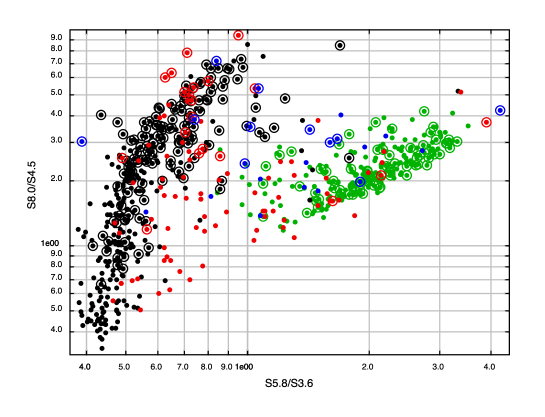
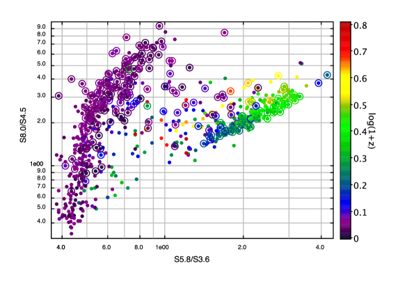
Figure 2: IRAC colour-colour plot (S_8.0/S_4.5 versus S_5.8/S_3.6) illustrating the objects of all the samples detected in the four IRAC bands. Left panel: the samples in black, red, and blue are the low-$z$, COSMOS, and ELAIS, respectively. The quasar sample (green) is shown for comparison. The points inside open circles denote detections at 70µm. The right panel shows the same diagram but with the colours of the points indicating their redshift.

One should keep in mind that the various samples have not only different observed properties but also very different average redshifts, as seen in the right panel of Fig. 2. A histogram of the redshift distributions is shown in the upper panel of Fig. 3. The middle and lower panels of Fig. 3 show the distributions of the 3.6 and 24 µm luminosities of the various samples.

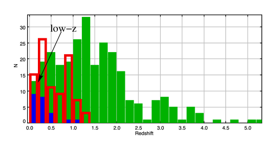
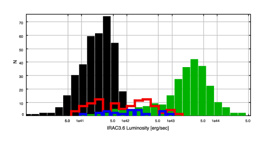
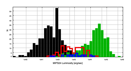
Figure 3: Redshift (upper panel), 3.6 µm luminosity (middle panel) and 24 µm luminosity (lower panel) histograms for for the low-$z$, COSMOS, ELAIS and quasar samples. Colour coding follows Fig. 2. The black arrow indicates the location of the low-$z$ sample.

3 OBSERVED AND MODEL SEDS

The observed UV to FIR SED of a galaxy can be decomposed in three distinct components: stars with the bulk of their power emitted in the optical and near-IR, hot dust mainly heated by UV/optical emission from gas accreting onto the central supermassive black hole and whose emission peaks somewhere between a few and a few tens of microns, and cold dust principally heated by star formation. In the present work we consider all three components, which we model as follows.

3.1 The stellar component

The stellar component is the sum of Simple Stellar Population (SSP) models of different age, all having a common (solar) metallicity. The set of SSPs is built using the Padova evolutionary tracks (Bertelli et al., 1994), a Salpeter IMF with masses in the range 0.15 – 120 M_⊙ and the Jacoby et al. (1984) library of observed stellar spectra in the optical domain. The extension to the UV and IR range is derived from the Kurucz theoretical libraries. Dust emission from circumstellar envelopes of AGB stars has been added by Bressan et al. (1998). The weight in the final spectrum of each SSPs, as a function of age, is computed according to a Schmidt law for the star formation rate:

$$SFR(t)=\left(\frac{T_{G}-t}{T_{G}}\right)\times\exp\left(-\frac{T_{G}-t}{T_{G}\cdot\tau_{sf}}\right)$$ (1)

where $T_{G}$ is the age of the galaxy (i.e. of the oldest SSP), which is assumed to be as old as the age of the universe at the galaxy’s redshift, and $\tau_{sf}$ is the duration of the burst in units of $T_{G}$. Extinction is applied to the final SED by assuming a uniform foreground dust screen with a standard Galactic extinction law (Cardelli et al., 1989). The free parameters are, therefore, the duration of the initial burst and the amount of extinction.

3.2 The torus component

The models for dust emission in AGN are those presented in Fritz et al. 2006. To summarize, the dust distribution is smooth, the torus geometry is that of a “flared disk”, the dust consists of graphite and silicate grains. The graphite grains, with sublimation temperature around 1500 K are responsible for the black body like emission in the near-IR part of the AGN spectra, creating a minimum in the observed SEDs between the falling accretion emission and the rising torus emission, while the silicate grains are responsible for the absorption feature at 9.7 micron, seen in the IR spectra of all type 2 AGN. The size of the inner torus radius, $R_{in}$, depends both on the sublimation temperature of the grains, $T_{1500}$, and on the accretion luminosity, $L_{acc}$, according to Barvainis (1987):

$$R_{in}\simeq 1.3\cdot\sqrt{\rm L_{acc}}\cdot T_{1500}^{-2.8}[pc]$$ (2)

The dust density within the torus is allowed to vary along both the radial and the angular coordinates:

$$\rm\rho(r,\theta)=\alpha\cdot r^{\beta}\cdot e^{-\gamma|\cos(\theta)|}$$ (3)

We give here, as a reminder, the parameter values for the discrete grid of torus models that will be used, as presented in Paper 1: $\beta=0.0,-0.5,-1.0$ and $\gamma=0.0,6.0$ (see Eq. 2), optical depth $\tau_{9.7}=1.0,2.0,3.0,6.0,10.0$; torus opening angle $\Theta$=20^o, 40^o, 60^o; and outer-to-inner radius ratio $R_{out}/R_{in}$=30 and 100. This last set of parameters only holds when $\beta=0.0$, i.e. when the dust density is constant with the distance from the centre. For the models with $\beta<0.0$, $R_{out}$ is re-calculated to be the distance at which the dust density drops at 10% of its value at $R_{in}$.

3.3 The starburst component

For the cold dust component, which is the major contributor to the bolometric emission at wavelengths longer than $\sim 30$ µm, we choose six well-studied observational SB templates: M82 as a representative of a “typical” SB IR emission, Arp 220 as representative of a very extinguished starburst and the templates of NGC1482, NGC4102, NGC5253 and NGC7714, as intermediate SB templates.

3.4 Fitting the observed SEDs

The SED fitting procedure is that of a standard $\chi^{2}$ minimisation. As a first step, the UV to near-IR (rest-frame) data points are fitted by means of a stellar host component that dominates the emission in this range (since the accretion emission of the low luminosity AGN of the sample is most probably masked under the stellar light). The best fit to the observed data points in this wavelength range is found by exploring a grid of $\tau_{sf}$ and $E(B-V)$ values (see Sec. 3.1).

In the next step, the mid-IR points are then fit by a torus component. Since all the objects under study are type 2 AGN and therefore the central source is hidden behind the torus, we will focus on the results of the run realised with torus models of high optical depth, $\tau_{9.7}\geq 1.0$ with the exception of the low-$z$ sample, for which we will allow a full run, including $\tau_{9.7}<1.0$ torus models, since for these low luminosity objects obscuration might also be the result of the dust in the host galaxy. In order to properly constrain the part of the SED where the cold dust is dominant, one would need at least one FIR measurement, in this case a 70 and/or 160 µm detection (the mid-Infrared 24 µm point alone is probably not enough to distinguish between a torus-like and a starburst-like emission). Correspondingly, an SB component will only be allowed in the presence of a 70 (and/or 160) µm datapoint(s), along the lines of Paper 1. A single deviation from this will be discussed in Section 4.1.

As detailed in Paper 1, the SED fitting leads to the computation of a series of physical parameters, namely the accretion luminosity, $L_{acc}$, the IR luminosity, $\rm L_{IR}$, integrated between 1 and 1000 µm, the inner and outer torus radii, $R_{in}$ (defined in Eq. 2) and $R_{out}$, the optical depth (or extinction) and hydrogen column density along the line of sight, the covering factor, CF, i.e. the fraction of the radiating source covered by the obscuring material, and the mass of dust, $M_{Dust}$. A quantity that was not dealt with in Paper 1 due to the nature of the sample (type 1 quasars and hence almost complete lack of stellar components) is the stellar mass, $M^{*}$, derived directly by the SSPs, that we will also include in the analysis of the low-$z$ sample.

For the degeneracies related to the various torus models parameters and the limitations inhibited in our approach, we defer the reader to sections 5.6 and 6 of Paper 1, where all these issues were discussed in detail. Dealing with quasars, the stellar and SB components were of secondary importance. In the present study, however, these two components play a more important role. The stellar component (SSPs), even though used to fit mainly the UV-to-optical part of the SEDs whenever necessary, is not studied any further and therefore discussing degeneracies between the relevant parameters is well outside the scope of this work, but a relevant discussion can be found in Berta et al. (2004). The only remaining issue is that of the normalisation of the SB template, particularly in the absence of a sufficient number of data points. After an initial normalisation of the mentioned temlpate to the 70 µm point, an iterative process results in the best normalisation factor after the torus emission has been excluded. In other words, the SB template is finally used to fit the emission that is not accounted for by the torus model. This could introduce a bias, maximising the estimated AGN and minimising the SB contributions, respectively. However, since the iterative process takes into account not only the best fit torus model but the best 30 torus models, we are confident that these deviations will not be more than a few percent.

4 TESTING THE INDIVIDUAL SAMPLES

4.1 Low-luminosity, low-redshift AGN

The distribution of the reduced $\chi^{2}$ of the sample is very broad and in general the values are quite large (Fig. 4, plain line). The reasons for these high values has been explained in detail in Paper I and relate, among other things, to the small values of the photometric errors as well as the crudeness of the X-ray-to-optical spectrum of the AGN models.

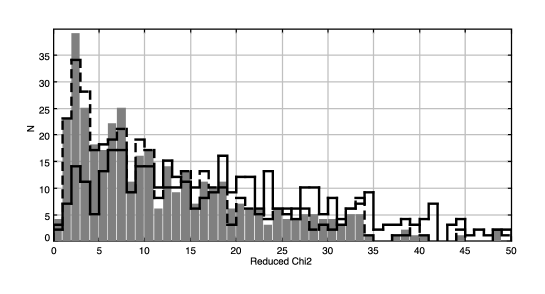
Figure 4: Distribution of the minimum $\chi^{2}$ from the analysis of the low-$z$ sample from the “standard” run when no SB component was allowed in the absence of 70 (and/or 160) µm data (plain line) and from the run allowing an additional SB component in the presence of a 24 µm detection (dashed line). In gray, is the final $\chi^{2}$ distribution selecting, for each object, the minimum $\chi^{2}$ between the two runs.

Examples of the observed SEDs and the best fit models for objects assigned a torus template are shown in Fig. 5. The sequence number (SqNr) shown in the plots correspond to the SqNr shown in table 1. The signature of a torus would be a large increase of the 24 µm flux with respect to the 8.0 µm point while the presences of a starburst will usually be revealed by a rise in the 8 µm flux due to the PAH features, but with a subsequent flattening or slow rise of the SED towards the redder (24 µm) wavelength. The absence of any component other than the stellar is marked by a monotone decrease of the SED after the stellar near-Infrared bump ($\sim 2-3$ µm ). The best fits for all 388 objects are provided as online material.

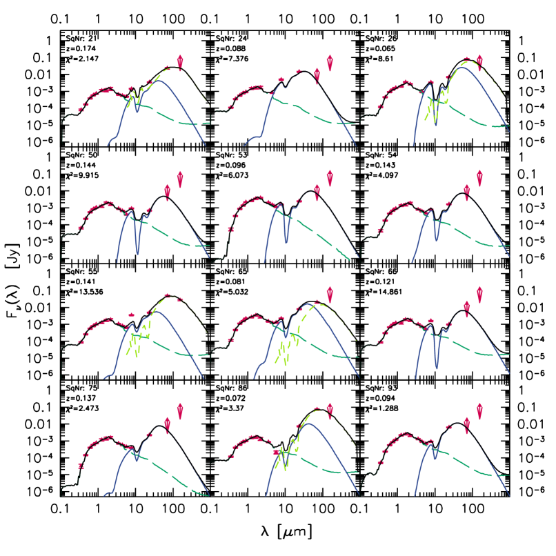
Figure 5: Best fit SEDs for the first 12 low-$z$ objects with reduced $\chi^{2}<16.0$ that were assigned a torus component. Data points (in the rest frame) are shown in red; the stellar model denoted with a green dashed line, the torus with a blue line, and the cold dust component with a dashed light green line.

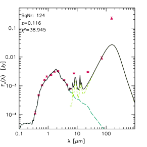
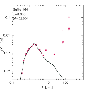
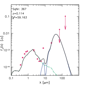
Figure 6: Examples of failed fits for three objects in the low-$z$ sample.

In Fig. 6 we also provide three examples of objects for which the fitting method completely failed to reproduce the observed SEDs, in order to give the reader a flavour of the various problems we have encountered. Object with SqNr 124 (left plot in Fig. 6) has very strong mid-to-far infrared emission that none of our SB templates was able to account for; object 164 (middle plot) has a stellar-like SED up to 5.8 µm, but the subsequent rise in flux at 8 µm and drop at 24 µm can not be reproduced by any combination of torus and/or SB templates; and the fitting method simply did not work for object Nr 367 (right plot), where both the assigned SSPs and the torus model reproduce very poorly the observed SED.

Going back to the best fits now, there is a correspondence between the weighted contribution of the various model components and the IRAC colours of the objects. Fig. 7 illustrates the position of the objects on the IRAC colour diagram (as in Fig. 2). In agreement with the predictions (e.g. Sajina et al. 2005) almost all objects assigned a stellar component alone are gathered at the lower left part of the diagram (stars), starbursts (large open circles) form the bulk of the sample and AGN (objects with a torus component shown as small filled circles) occupy the space towards the upper right part of the diagram. Note however, the large overlap between SBs and stellar-dominated galaxies, which suggests their close physical relationship and fitting redundancy between these two types of galaxies.

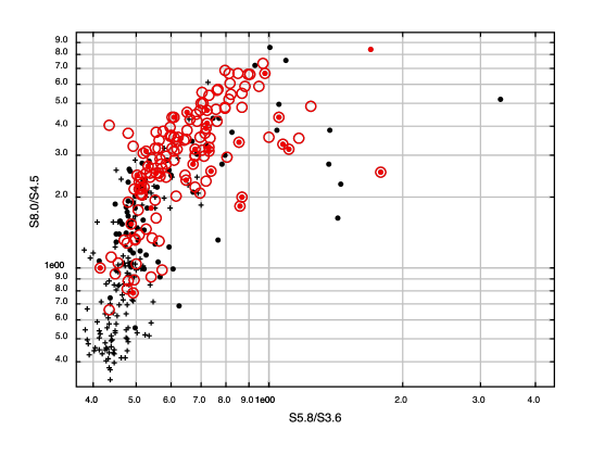
Figure 7: IRAC colour-colour diagram (see Fig. 2) indicating the objects with a stellar component alone (stars), with a torus component (small filled circles) and a starburst component (large open circles). The symbols in red represent objects with a 70 µm cold dust component.

Drawing a conclusion on the nature of the objects with no 70 µm detection is actually not straight forward. There are cases where the IRAC fluxes are monotonically decreasing, tracing unmistakably the stellar emission. While in other objects the 8 and/or 24 µm flux is slowly increasing (unlike a torus signature), indicating the presence of a starburst, yet no FIR is detected for some of these cases. Objects with predominantly, starburst as opposed to AGN activity and SEDs dominated by emission in the MIR ($\sim 24$ µm) rather than the FIR ($\lambda\geq 60$ µm) are actually known to exist (see e.g. Engelbracht et al. 2008).

The observed SEDs of these objects were poorly reproduced with the combination of a stellar and a torus components alone. As a test, and conversely to the process followed in Paper I, we performed an extra run allowing for the use of an SB template even in the absence of a 70 µm detection. The results of this run should, therefore, influence the objects without 70 µm counterparts, representing however the majority (2/3) of the sample. The distribution of the reduced $\chi^{2}$ for this run, shown by a dashed line in Fig. 4, is narrower than that of the “standard” run, peaking at $\chi^{2}\sim$ 2. This improvement comes mainly from better fitting the 8 and/or 24 µm points of the objects that were only assigned a stellar component, by an additional SB component. In order to combine the results of the two runs, we will simply select the best $\chi^{2}$ from the two runs, shown in Fig. 4 with a gray histogram. For consistency with the study in Paper 1 we will consider “good” all fits with $\chi^{2}<16$, whose limit includes $\sim$70% of the sample. Note, however, that we run the same analysis on the entire sample (388 objects) and found none of the results differ in any way if all fits are included.

The sample of objects harbouring an AGN according to the present analysis, shows very specific trends: the majority of objects (87%) were assigned very high optical depth tori ($\tau_{9.7}=10.0$), and 90% were assigned tori models with decreasing dust density from the centre ($\beta<0.0$ in Eq. 3). In fact, there is a clear preference for models with $\beta=-0.5$, with 72% of the objects assigned such a torus component. Almost 85% of the sample have small outer to inner radius ratio ($R_{out}/R_{in}=30$). The combined result is very small tori with inner radii of less than 1.4 pc ( 0.185 pc average) and outer radii reaching in a few cases 100 pc. These average values are $\sim$2 times smaller than the average values for $R_{in}$ derived for the quasars and reflect the lower average accretion luminosity, $L_{acc}$, of the low-$z$ sample. In fact, the lower (by a factor of $\sim$25) $\langle L_{acc}\rangle$ of this sample with respect to the quasars is not only due to the different redshift ranges covered by the two samples but also to the very nature of the objects.

The contribution of the AGN to the IR luminosity, for the 75 “good” fits that have been assigned a torus component, is shown in Fig. 8, with the grayed-out region corresponding to the 20 objects with an extra SB component. Due to the nature of the objects the AGN fraction tends to be very low compared to the values derived from the SWIRE/SDSS quasar sample of Paper 1.

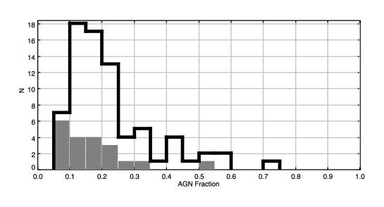
Figure 8: Histogram of the fraction of IR luminosity attributed to the AGN, for objects assigned a torus component (open histogram) and those with an extra SB component (gray region).

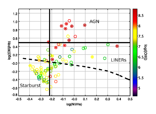
Figure 9: Emission line ratios as a function of extinction corrected [Oiii] line luminosity, for those objects with a 70 µm counterpart. Large open and small filled circles denote SB and torus component, respectively. The dashed line shows the usual - and more conservative - AGN selection criterion suggested by Kewley et al. (2001), according to which the AGN should occupy the upper right part of the graph.

All 91 objects with a 70 µm detection, for which the fits are optimally constrained, were assigned a starburst component; of that total, 20 of them show evidence for the presence of a torus. Fig. 9 depicts the relative intensities of emission lines (log([Oiii]/H$\beta$) versus log([Nii]/H$\alpha$), as a function of the extinction corrected [Oiii] luminosity. Six of nine objects that occupy the space commonly agreed to be populated by Seyfert 2 galaxies (upper right corner in Fig. 9) have indeed been assigned an AGN component. Another four lie very close to the dividing lines, and a total of six in the LINERs’ region (lower right part). The majority of the objects were assigned an SB component alone and would have not been part of the AGN catalogue at all, had the Kewley et al. (2001) AGN selection criterion been applied (shown here in a dashed line).

The average values for the [Oiii] luminosity and the log([Oiii]/H$\beta)$ ratio for the objects with an AGN component, an additional SB component and an SB component alone are given in table 5. Both quantities have larger values when an AGN component is present and lower when an SB component alone is responsible for the cold(er) dust emission.

Table 5: The average values for the [Oiii] luminosity and the log([Oiii]/H$\beta)$ ratio for the objects with an AGN component, an additional SB component and an SB component alone.

Component	#	log([Oiii])	log([Oiii]/H$\beta$)
AGN	20	8.18 $\pm$ 0.60	0.299 $\pm$ 0.42
AGN $+$ SB	91	7.38 $\pm$ 0.75	0.006 $\pm$ 0.37
SB alone	71	7.16 $\pm$ 0.64	-0.077 $\pm$ 0.31

Our analysis is only able to identify a torus component in about one-third of the total low-$z$ sample (75 [142 if no cut in the $\chi^{2}$ is imposed] out of 266 [388]). Even though evidence of changing behaviour of (clumpy) tori (Hönig & Beckert, 2007) or even complete disappearance of the torus (Elitzur & Shlosman, 2006) towards the lower luminosity regimes ($L<10^{42}$ erg/sec) has been reported, these effects are not what we observe here, as the lowest accretion luminosity estimated for objects with a torus component is of the order of 10⁴⁴ erg/sec, seen in the first plot of Fig. 18. We therefore conclude that we either are unable to detect the signature of AGN with $L_{acc}<10^{44}$erg/sec or that the criteria used by Kauffmann et al. (2003) to select AGN were too generous and many objects with no nuclear activity may have made it into the suggested AGN sample.

Another issue to consider is the distribution of the resulting covering factor, shown in Fig. 10. Were the computed values for CF correct, they would translate to a ratio of type2:type1 objects of about 1:1 in the local and low-$z$ universe, a much lower value than that observed.

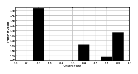
Figure 10: Covering Factor distribution for the low-$z$ sample.

This discrepancy could again be seen as a result of the AGN candidate selection and the somewhat sparse samples of the observed SEDs, the combination of which does not always allow the fitting code to give robust results.

Allowing for torus models with $\tau_{9.7}<1.0$ does not have any effect on the results, as only 18 out of the 388 objects where better fit by a model including such a torus component, with a single one among them assigned a $\chi^{2}<16.0$.

4.1.1 Properties of the host galaxies

The SSPs used to reproduce the blue part of the SEDs provide information about the stellar mass of the host galaxy. To compute the stellar mass we exploit the fact that SSP spectra are given in luminosity units per one solar mass. We also account for the fact that a certain percentage of stars, depending on the SSP’s age, has evolved and is not shining anymore, so the mass value we provide is actually “luminous mass”, Fig. 11 shows a comparison of the stellar mass computed in this work and that provided in the narrow line AGN catalogue Kauffmann et al. (2003). The line shows the linear correlation between the two quantities, $M^{*}_{here}$ = 1.59 + (1.06$M^{*}_{\bf K}$). Note that the systematic differences in the mass values are the result of the different IMF used by Kauffmann et al. (2003), a Kroupa (2001) IMF, which differs from ours both in the slope and in the mass limits.

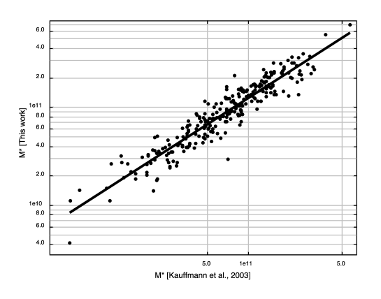
Figure 11: Comparison of the stellar mass derived from this work based on SED fitting and that presented in Kauffmann et al. 2003.

We now compute the star formation rate (SFR) according to Kennicutt (1998) as

$$SFR[M_{\odot}/yr]=4.5\times 10^{-44}\times L_{FIR}$$ (4)

where $L_{FIR}$ is the infrared luminosity of the SB component, integrated between 8 and 1000 micron. Fig. 12 shows the distribution of the SFRs for all objects with an SB component and $\chi^{2}<16.0$ (black histogram), with the grayed region corresponding to the objects without an AGN component. The average SFR of the entire sample without imposing a cut on the $\chi^{2}$ values is of 2.8 $M_{\odot}$/yr, and drops to 2.2 when only objects with $\chi^{2}<16.0$ are consider, and to 1.85 when objects with an AGN component are excluded.

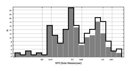
Figure 12: Star formation rates for all objects with an SB component and $\chi^{2}<16.0$ (black histogram) and those without an AGN component (gray histogram).

Note that all objects with a torus component are gathered in the part of the histogram with the higher SRFs. We will get back to the discussion on SFRs in Section 5.4.

4.2 Type 2 AGN and hybrids from the COSMOS sample and Mid-IR selected ELAIS AGN

The spectroscopic sample of X-ray emitters selected in the COSMOS field presented in Trump et al. (2007) comprises 80 type 2 AGN, 47 type 2 AGN and red galaxy hybrid and 8 type 2 AGN whose classification is not 100% secure. Ninety two out of these 135 objects have a 24 micron counterpart and, as already mentioned in Section 2, we will be concentrating on this sub-sample alone. This was not a constraint applied to the low redshift sample, however, due to the average (low) redshift of this sample as well as its nature (see Fig. 3). The SEDs are dominated by the stellar light all the way to the IRAC3 band (5.8 µm) and even though the presence of a torus is somewhat revealed from the lower S_8.0/S_5.8 colour (with respect to objects without a torus component), a single data point at 8.0 µm (IRAC4) is not enough to constrain the torus properties. For the record, 36 of the remaining objects (those without a 24 µm detection) were indeed assigned a torus component while six others were better represented by SSPs alone.

Fig. 13 shows the minimum $\chi^{2}$ distribution for the sub-sample of 92 objects whose SEDs extend at least up to 24 µm, (solid line), excluding two objects with minimum $\chi^{2}>90$ that are obviously erroneous and will not be taken into account in what follows. Again for consistency, we will adopt a cut-off $\chi^{2}$ of 16, keeping in mind though that including the rest of the fits will not influence the results in any significant way.

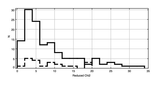
Figure 13: Histogram of the minimum $\chi^{2}$ from the analysis of the COSMOS (solid line) and the ELAIS (dashed line) samples.

Examples of SED fits of objects assigned an AGN component are shown in Figs. 14 and 15, for the COSMOS and ELAIS samples, respectively. The fits for all objects are available as online material.

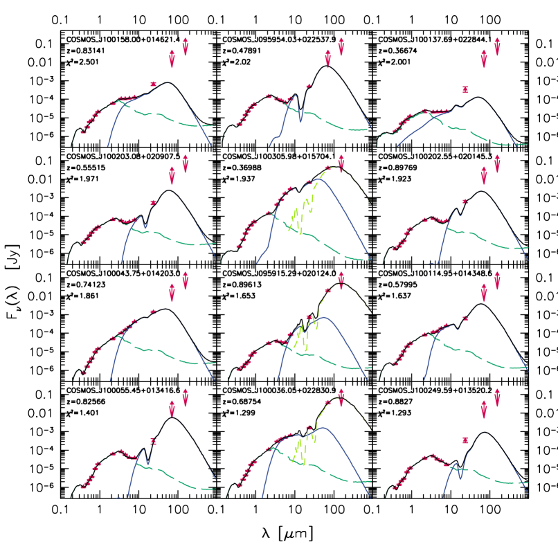
Figure 14: The best fits for the first 12 COSMOS objects with reduced $\chi^{2}<16.0$ that were assigned a torus component. Data points (in the rest frame) are shown in red; the stellar model denoted with a green dashed line, the torus with a blue line, and the cold dust component with a dashed light green line.

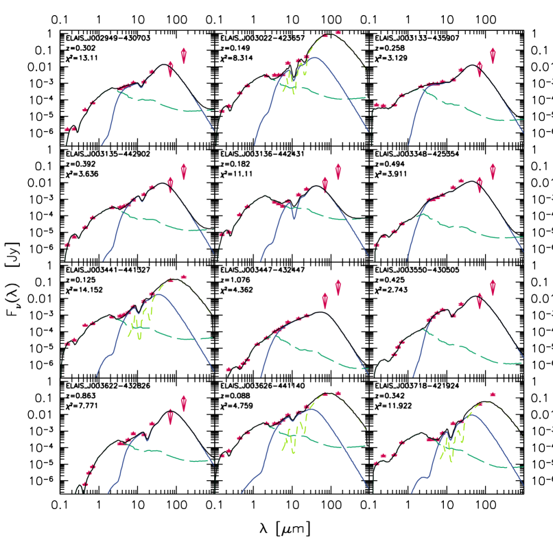
Figure 15: The best fits for the first 12 ELAIS AGN with reduced $\chi^{2}<16.0$ that were assigned a torus component. As in Figs. 5 and 13, data points are shown in red; the stellar model is marked with a green dashed line, the torus with a blue line, and the cold dust component with a dashed light green line.

Note that in the upper and lower left plots in Fig. 14 (objects COSMOS_J100137.69+002844.1 and COSMOS_J100249.59+013520.2, respectively), the observed 24 µm points lie well above the model (in both cases consisting only of stars and a torus). Such cases indicate the possible existence of an additional SB component, which we did not use for these fits because of the lack of observed 70 and/or 160 µm data points, as discussed in detail in Section 3.4. Similarly, for the lower right object in Fig. 15 (ELAIS_J003718-421924), the fit fails to reproduce the 160 µm point, despite the simultaneous existence of a torus and a SB components. This case shows that either the SB templates used are not always adequate or, most probably, that we are lacking a diffuse component that would account for the cold dust in the host galaxy.

The fitting results show a clear preference for models with dust density decreasing with the distance from the centre, with 95% of the objects finding a better fit with $\beta<0.0$ models (75% with $\beta=-0/5$). A further dependence of the dust spatial distribution on the altitude from the equator was found, with 87% of the objects having a best fit model with $\gamma=6.0$. The resulting tori sizes do not depend on the type of object (AGN or hybrid) and the estimated average inner tori radii, $R_{in}$, are of 0.85$\pm$0.50 and 0.91$\pm$0.58 pc, for AGN and hybrids, respectively, and with about 60% of the objects better matching torus models with small sizes ($R_{out}/R_{in}$=30). More than half of the objects were found to have a large covering factor ($>80$%). A comparative study on the covering factor derived from the various samples will follow shortly.

Once again, the position of the objects in the IRAC colour diagram (Fig. 2) and the contribution of the various components in their global SEDs are in very good agreement. Fig. 16 shows the IRAC colour diagram for the COSMOS (circles) and ELAIS (squares) samples.

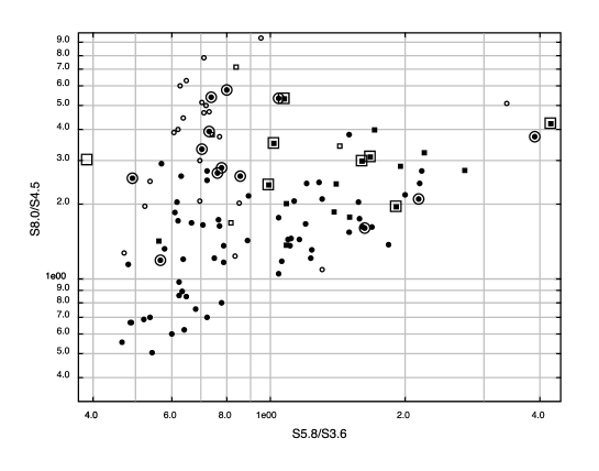
Figure 16: IRAC colour diagram for the COSMOS (circles) and ELAIS (squares) AGN. Small filled symbols denote an AGN component, large open symbols an SB component, for objects with a good $\chi^{2}$. Small open symbols mark the objects whose fits were not acceptable.

The majority of objects with a 70 micron detection and an assigned SB template gather in the PAH-dominated locus (upper left part of the diagram) while the AGN contribution to the IR luminosity increases as objects move along the continuum-dominated locus, becoming redder in the $S_{5.8}/S_{3.6}$ axis.

From the 23 objects composing the MIR selected type 2 ELAIS AGN sample, 21 were found to have a torus component, all of which with $\tau_{9.7}\geq 6.0$, $\gamma$=6.0 and $\beta<0.0$, among which 15 found a better fit with $\beta=-0.5$ templates. The average estimated sizes of the tori were very similar to those of the COSMOS sample. The reduced $\chi^{2}$ distribution for the fits is shown in Fig. 13 in dashed lines.

The AGN contribution to the IR luminosity for both samples is shown in Fig. 17, with the grayed region representing the objects with an additional SB component. The plain (dashed) line and grayed (black) region correspond to the COSMOS (ELAIS) sample. Again, the existence of such a component can be, in general, well constrained only in the presence of data points longward $\lambda=24$µm and this is valid for only 25% and 50% of COSMOS and ELAIS samples, respectively.

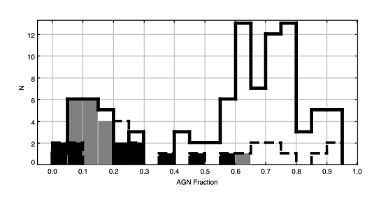
Figure 17: Histogram of the fraction of IR luminosity attributed to the AGN, for objects from the COSMOS and ELAIS samples..

5 COMBINED AGN PROPERTIES

We will now attempt to put all the results from the various AGN samples together and construct a common description of their dust properties. To this end, we will first present a summary of the results of Paper 1, that will also be used in this combined study. The low-$z$ sample will be excluded from this analysis, because of the unconfirmed (stellar vs. starburst) nature of the objects. They will be taken into account, however, when discussing the star formation, as the results on this issue seem to be more robust, and only marginally affected by the presence of tori, as suggested from Fig. 8.

5.1 Type 1 SWIRE/SDSS quasars

Paper 1 focused on the study of 278 SDSS/SWIRE quasars and the properties of dust surrounding them. Comparing the results between the “restricted” run, where only high $\tau_{9.7}$ models were allowed and the “full” run, where optical depths as low as 0.1 were allowed, the hypothesis of the existence of low optical depth tori could not be ruled out. In fact, the majority of objects found a better match of their SEDs with low $\tau_{9.7}$ models ($\tau_{9.7}<1)$. The computed average inner radius was of $\sim$2.6 pc with a tendency for higher $R_{out}/R_{in}$i (=100) for the full run (59%) with respect to the restricted run (46%), as reported in Paper 1. The covering factor depended of course on the choice of the optical depth but had a relatively flat distribution in both cases, taking values from as low as $<0.1$ to as high as 0.95. As for the dust density, there was no clear preference between $\gamma=0.0$ and $\gamma=6.0$ models, in any of the runs, while $\beta<0.0$ models were always favoured. The accretion and IR luminosities were the two better constrained quantities and were almost independent on the choice of $\tau_{9.7}$. The subsample of 70 objects with 70 µm detections enabled an estimation of the contribution of a starburst to the total IR luminosity, indicating contributions of up to 80%.

5.2 Comparative study of type 1 & 2 AGN

Section 2.3 described the observed properties of the combined AGN sample. Although the sample is not complete, the combined study of the various AGN sub-samples composing it, will allow for comparative conclusions.

Fig. 18 shows the distribution of the various parameters for the different samples. From top to bottom and left to right, and following the colour-coding introduced in the left panel of Fig. 2 we present: the accretion luminosity; and the IR luminosity attributed to the torus component (i.e. excluding the stellar emission coming either from the SSPs and/or the SB components); the covering factor; the viewing angle; the hydrogen column density along the line of site; and the mass of dust confined inside the torus. The open histogram corresponds to the “restricted” run, where only high optical depth tori models ($\tau_{9.7}\geq 1.0$) were allowed (Paper 1).

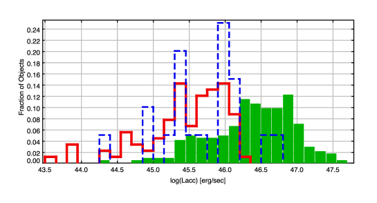
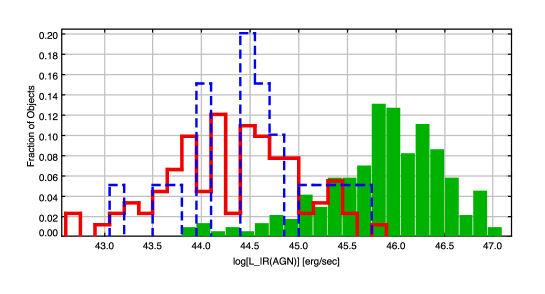
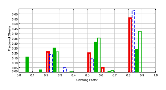
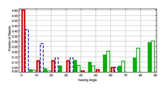
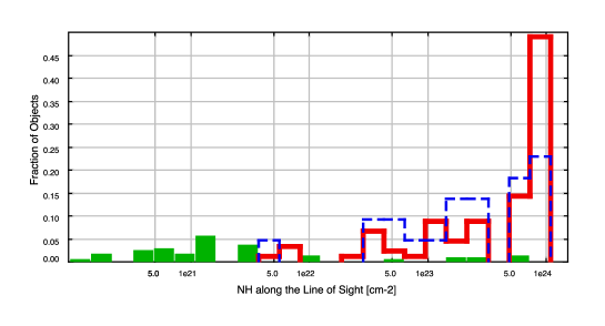
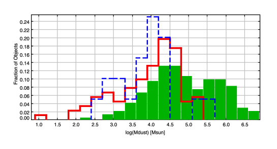
Figure 18: From top to bottom and left to right: accretion luminosity, $L_{acc}$, and infrared luminosity attributed to the AGN component, covering factor, viewing angle, hydrogen column density, and mass of dust, for the various samples. Green filled and empty histograms show the distributions for the quasar “full” and “restricted” runs, respectively; red open full-line and blue dashed-line histograms show the results for the COSMOS and ELAIS samples, respectively. The low-$z$ sample has been excluded.

The combined quasar and type 2 AGN samples cover four orders of magnitude in $L_{acc}$, with the quasar $L_{acc}$ distribution peaking at luminosities of about an order of magnitude brighter than the type 2s (see Fig. 18 - upper left). This observational bias affects, for example, the fraction of the IR luminosity attributed to the torus component (Fig. 18 - upper right).

The viewing angle as derived from the fits, shown in the right column, second row, is consistent with the Unified Scheme postulating that the differences between type 1 and type 2 objects are a line-of-sight effect, with the type 2 objects seen through the obscuring material. Almost all type 2 objects are seen in small viewing angles, i.e. close to the equator and through large amounts of dust, while type 1 objects are seen in large viewing angles especially when only tori with high optical depths are considered (open green histogram). Note that low optical depth tori would result in low obscuration type 2 AGN when seen edge-on. Fig. 4 in Fritz et al. (2006), e.g., shows the emission of an AGN through a $\tau_{9.7}=0.1$ torus for all lines of sights. While the object is clearly a type 1 when seen face-on, the UV-to-optical nuclear emission can be absorbed by several orders of magnitude when seen through the dust, depending on the wavelength and the line of sight.

The majority of type 2 objects are seen through high column densities ($N_{H}\geq 10^{23}cm^{-2}$), while the few quasars that are seen through the torus, are actually seen through low optical depth and lower than the type 2 column density gas (Fig. 18, lower left panel). Also consistent with the Unified Scheme is the distribution of the mass of dust (right column, fourth row in Fig. 18). If the mass of dust can be considered a linear tracer of gas, this implies that the gas reservoirs in the vicinity of type 1 and type 2 objects are comparable.

Note that the properties of the radio and X-ray (COSMOS) and MIR-selected (ELAIS) AGN are remarkably similar with the only notable difference being the slightly higher IR luminosities of the torus components of the ELAIS sample (upper right plot in Fig. 18), simply reflecting the selection effects.

5.3 The covering factor

The distribution of the values for the covering factor (seen in the left column, second row in Fig. 18) indicates that tori with both high and low covering factors are possible in both types of objects. The COSMOS and ELAIS samples show a stronger tendency for higher values.

The estimated type2:type1 ratios based on the CF distribution of the type2 objects is $\sim$2-2.5:1; the same ratio is found when considering the restricted run of the quasar sample. The full type 1 run, however, suggests a ratio of 1:1, with a mean value of the covering factor of $\sim$0.47, very close to the value of 0.4 computed by Rowan-Robinson et al. (2008) for the entire SWIRE quasar population. This low value, seemingly in conflict with the Unified Scheme, actually reflects the difference in the accretion luminosity between the type 1 and type 2 samples (Fig. 18), already discussed in Section 5.2.

From the type 1 quasars with redshifts below $\sim 0.8$ we can measure the flux at 5100 Å, which we can then scale with the accretion luminosity, $L_{acc}$, as seen in the left panel of Fig. 19. Assuming this relation holds for all redshifts as well as for type 2 objects, we can translate $L_{acc}$ to $L_{5100}$. We can then compute the fraction of obscured AGN in bins of $L_{5100}$, shown in the right panel of Fig. 19. The black circles and open squares make use of the results of the full and restricted runs, respectively. The full and two dashed lines show the results and uncertainties (due to bolometric corrections) obtained by Maiolino et al. (2007) who conducted a study of 25 high luminosity high redshift ($2<z<3.5$) quasars with IRS spectroscopy. The observed trend, i.e. the decreasing average torus covering factor with increasing AGN luminosity, is in support of the receding torus paradigm, suggested by Lawrence A. 1991.

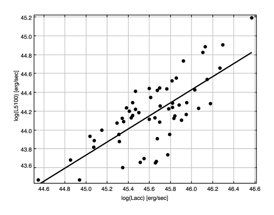
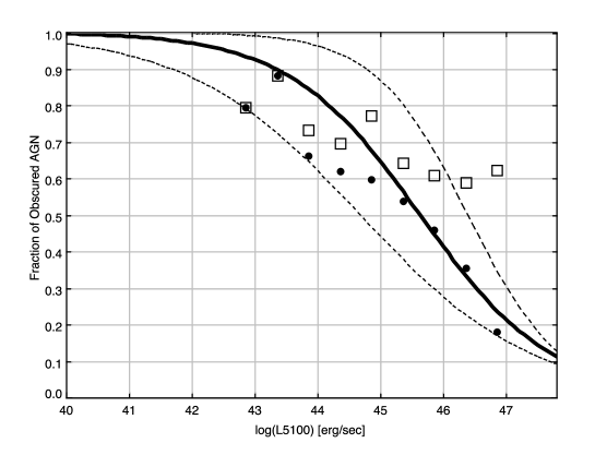
Figure 19: Left panel: $L_{5100}$ measured on the quasar SDSS spectra for objects with redshift lower than $\sim$0.8, versus $L_{acc}$, computed from the SED fitting. The linear correlation, shown in a solid line, is given by $log(L_{5100})=0.692\times log(L_{acc})-1.5767$. Right panel: fraction of obscured AGN in bins of $L_{5100}$. Filled circles (open squares) represent the results of the full (restricted) run. The solid line represents the fraction of obscured AGN as found by Maiolino et al. (2007), while the dashed lines trace the uncertainties due to bolometric corrections.

Despite the crude conversion of $L_{acc}$ to $L_{5100}$ our results making use of the full run are in very good agreement (i.e. within the uncertainties) with those derived by Maiolino et al. (2007) based on totally independent method and sample, while the results based on the restricted run, even though still consistent (excluding the brightest two bins) show a quite different trend. We can therefore still not conclude on the relative occurence of low $\tau_{9.7}$ tori with respect to high $\tau_{9.7}$ tori but, based on the above, we can still provide some evidence for their existence.

Previous studies (e.g. Maiolino et al. 2007) assume that the ratio between the primary AGN radiation (here measured by $L_{acc}$) and the thermal infrared emission attributed to the AGN is a direct indicator of the torus covering factor. Our findings confirm this assumption, as shown in Fig. 20 where the accretion-to-IR AGN luminosity of each individual object of each sample is plotted against the computed covering factor. The slope of the correlation is very similar for type 1 and type 2 samples. Type 2 objects, however, have considerably larger $L_{acc}/L_{IR}(AGN)$ ratios than the quasars. This “jump” in the values is due to the different viewing angles and occurs right when the line of sight intercepts the obscuring torus. In order to illustrate this effect, we show the $L_{acc}/L_{IR}(AGN)$ ratios as a function of the viewing angle for the extreme models of both type 1 and 2 objects (higher and lower red points; higher and lower green points in Fig. 20) in Fig. 21.

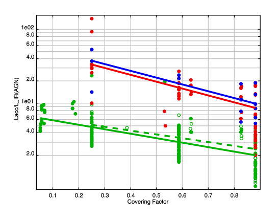
Figure 20: Accretion-to-IR luminosity attributed to the AGN component as a function of the covering factor. The green solid and dashed lines obtained as linear fits corresponding to the full and restricted runs, respectively, for type 1 objects, while blue and red lines correspond to ELAIS and COSMOS type 2 AGN, respectively.

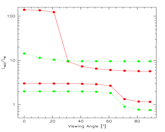
Figure 21: Accretion-to-IR luminosity attributed to the torus as a function of viewing angle for the type 1 (green dashed lines) and 2 (red solid lines) objects with the highest and lowest $L_{acc}/L_{IR}(AGN)$ in Fig. 19. The differences in this fraction are mainly attributable to dust self absorption which is more efficient for type 2 line of sights.

5.4 Starburst activity in AGN

The study of objects with at least one data point at wavelengths longward of $\lambda=24$ µm shows that the IR emission of AGN can not be attributed to the torus component alone. In the vast majority of cases, and in order to reproduce the 70 (and, whenever available, 160) µm points, an additional SB component was necessary. Furthermore, in all those cases the contribution of the AGN emission in the infrared is typically smaller than 50%, as seen in Figs. 8 and 17 for the type 2 objects, and a bit higher in type 1 quasars (Paper 1, Fig. 12).

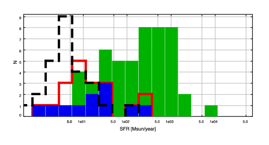
Figure 22: SFRs estimated from the Kennicutt (1998) formalism for the various samples.

Fig. 22 shows the estimated SFRs for the various samples (with the same colour coding as in Fig. 2) computed from Eq. 4 for all objects with an SB and an AGN components. The average SFR for the low redshift sample is about 10 $M_{\odot}$/yr, while those computed for the COSMOS and ELAIS samples are of $\sim$40 $M_{\odot}$/yr but with a larger span. That of type 1 quasars (shown in green), however, has an average SFR of 115 $M_{\odot}$/yr, with some cases reaching SFRs of the order of 10³ $M_{\odot}$/yr. These values are well in agreement with the findings of Serjeant & Hatziminaoglou (2009), a study based on stacking analysis of a variety of quasar samples. These values do not necessarily imply that star formation activity is stronger in type 1 quasars in general. More likely, it reflects the observational biases of the samples, both in terms of average redshifts and luminosities (Figs. 3 and 18).

The starburst-to-AGN luminosity ratio for the combined sample shows a slight tendency to decrease with increasing accretion luminosity, as seen in Fig. 23. This is in apparent agreement with previous works on type 1 quasars alone (again by Maiolino et al. 2007), and if confirmed for the entire sample, would imply that type 1 and type 2 objects behave in the same way in this respect. On the other hand, we can not assert beyond doubt that there there is no implicit dependency on the redshift. In fact, examining the quasar sample alone (open symbols) we would be tempted to claim an increase with $L_{acc}$, but which is likely attributed to the $L$ - $z$ degeneracy.

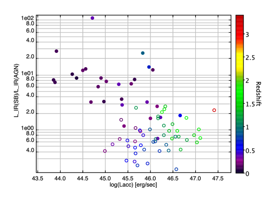
Figure 23: Starburst-to-AGN infrared luminosity ratio as a function of the accretion luminosity, $L_{acc}$, and the redshift. Filled and open symbols depict the type 2 and type 1 objects, respectively.

6 DISCUSSION

This work focuses on the IR properties type-2 AGN, the type 1 issues having already been discussed in a previous paper (Hatziminaoglou et al., 2008). The collection of data used for this paper comes from: 1) a low-redshift ($0.02<z<0.2$) AGN sample, selected via standard emission-lines ratios criteria; 2) a higher redshift ($0.1<z<1.4$) sample from the COSMOS and ELAIS fields, selected with X-ray and Mid-Infrared criteria. The observed SEDs were reproduced by means of a three component model, including emission from stars, hot dust from AGN and warm dust from starburst activity, and acceptable fits were obtained for the majority of the objects.

Despite the fact that the samples we analyzed were not chosen homogeneously, a comparison of the behaviour between the physical properties of the type 1 and type 2 AGN, shows an overall agreement. In Paper I we found the covering factor to have a broad trend towards lower values as the accretion luminosity, i.e. the power of the central engine, increased with small, on-average, covering factors. Applying the $L_{acc}$ versus $L_{5100}$ correlation derived for quasars in Paper I, we derived the flux at 5100 Å for the type 2 samples and checked the correlation between the optical luminosity and the covering factor, which in turn, can be converted into a type1-to-type2 fraction. The results provided by the SED fitting analysis, show a very good agreement with the relation presented in Maiolino et al. (2007), who find a correlation between the fraction of obscured AGN as a function of the optical luminosity (i.e. at 5100 Å). Another indication of the dusty torus was thought to be ratio between the accretion luminosity and the torus infrared luminosity. In fact, the latter is just reprocessed radiation which scales linearly with the primary source: what makes the difference is the fraction of “heating radiation” which is intercepted by the dust, which again depends on the covering factor. We find a very similar trend for these quantities, in both type 1 and type 2 objects, also showing how differences in the amount of obscuration are very well explained by dust self-absorption, i.e. thermal dust emission absorbed by dust iteself.

For the low-$z$ sample, we found no evidence of emission from an AGN component for $\sim 70$% of the objects. Although we cannot rule out the absence of an AGN from these sources, we can set an upper limit to its luminosity since it is not observed at mid-infrared wavelengths where its emission is the strongest as compared to both that of the stellar and of the starburst-heated dust. This sample suffers from high contamination from the stellar emission component, even at mid-infrared wavelengths where (on the contrary) it’s the AGN component that usually dominates when present. The question to ask, therefore, is what can be really constrained with three or four data points. One of the most reliable quantities should be the optical depth, since low values would make the torus emission stand over the stellar (SB or stars) in the MIR. In this respect, the low-$z$ sample may be too generous in selecting really active AGN. There is, sometimes, no evidence for a MIR excess at all with respect, for example, not only to a “normal” starburst emission, but also to a passively evolving galaxy. The absence of any evidence for a hot dust emission in the MIR, which is the place where the stellar component is less important and the AGN contribution is increasingly brighter, will remove the AGN component from the fits even though this could also be turned into an upper limit. In the cases where there is a MIR excess with respect to a pure stellar emission, we explore two possibilities: torus and PAH emission. In some cases a better fit was obtained adding PAH -i.e. starburst component alone- to the model instead of AGN which should instead dilute the PAH emission (Lutz et al., 1998).

Comparison between clumpy and smooth tori models (e.g. Dullemond & van Bemmel 2005) indicate that globally the SEDs produced by the two models are quite similar, but with some details characteristic for one or the other model: the silicate feature observed in absorption in objects seen edge-on is shallower for clumpy models, the average near-IR flux is weaker in smooth models and the clumpy models tend to produce slightly wider SEDs at certain inclinations. Furthermore, clumpy models can produce very small tori sizes with $R_{out}/R_{in}\sim 5-10$ (Nenkova et al., 2008), while still producing a broad MIR emission. Subsequently, the selection of a smooth torus for the present study might have resulted in overestimated tori sizes without, however, jeopardising the estimates on the properties related to the IR emission or our conclusions on the Unification Scheme. SED fitting may not be a sensitive enough method to distinguish between the differences introduced by the two approaches, because of the width of the filters and the scarce sampling of the observed SEDs, but also because the various characteristics of the torus component can be altered or diluted by, for example, the presence of a starburst component. Notwithstanding these limitations, SED fitting is still the best tool available for extracting the maximum information from large photometric AGN samples and is now proving to be a powerful technique in relating the dust properties to the accretion properties as well as the properties of the larger host galaxy.

Because AGN are of order hundred times less numerous than galaxies and also prone to selection biases, such AGN studies are only possible with the advent of multi-wavelength surveys that probe large volumes and allow the construction of well-samples SEDs. Even though we cannot address all issues related to dusty tori, our understanding of their properties has been greatly improved over the last decade thanks to the Spitzer Observatory. This space infrared telescope allowed, among other things, the construction of SEDs of hundreds of AGN of all types thanks to the IRAC and MIPS photometry (e.g. Franceschini et al. 2005; Hatziminaoglou et al. 2008; Richards et al. 2006; Polletta et al. 2008). Spitzer also opened the doors to detailed and coherent studies of the interplay between AGN and starburst activity (e.g. Hernan-Caballero et al. 2009 and references therein), paving the way for Herschel.

In fact, Herschel with its two cameras/medium resolution spectrographs (PACS; Poglitsch & Altieri 2009 and SPIRE; Griffin et al. 2009) and a very high resolution heterodyne spectrometer (HIFI; De Graauw et al. 2009) will be the first space facility to completely cover the range between 60 and 670, where the the bulk of energy is emitted in the Universe, allowing for a more detailed sampling of the observed FIR SEDs and the cold dust emission. Large parts of the Herschel key science will focus on the formation and evolution of galaxies and the studies of star formation. HerMES, the Herschel Multi-tiered extragalactic Survey, is the largest project that will be conducted by Herschel, with dedicated $\sim$900 hours that will map over 70 square degrees including most of the SWIRE fields (where most of the IR photometry of all the objects in this study comes from) as well as other extragalactic survey fields covered by several missions in all wavelengths (e.g. COSMOS or the Groth Strip), and will address among others the issue of AGN and starburst connection (Griffin et al. 2006; Hatziminaoglou et al. 2007). Additionally with Herschel, the Astrophysical Terahertz Large Area Survey (ATLAS) will cover about 500 square degrees and will observe all SDSS quasars with redshift $z<0.2$ as well as all the brightest FIR SDSS quasars (with luminosities 10 times larger than the mean), amounting to $\sim$330 individual detections of quasars in the area covered (Serjeant & Hatziminaoglou, 2009) (a factor of $\sim$5 more than all the SDSS quasars with 70 µm detections). These studies will allow us to significantly improve our understanding of the AGN phenomenon, disentangle the contribution of cold and hot dust emission in their SEDs and study the concomitant occurence of nuclear activity and star formation.

ACKNOWLEDGMENTS

This work is based on observations made with the Spitzer Space Telescope, which is operated by the Jet Propulsion Laboratory, California Institute of Technology under NASA contract 1407. Support for this work, part of the Spitzer Space Telescope Legacy Science Program, was provided by NASA through an award issued by the Jet Propulsion Laboratory, California Institute of Technology under NASA contract 1407.

Funding for the creation and distribution of the SDSS Archive has been provided by the Alfred P. Sloan Foundation, the Participating Institutions, the National Aeronautics and Space Administration, the National Science Foundation, the U.S. Department of Energy, the Japanese Monbukagakusho, and the Max Planck Society. The SDSS Web site is http://www.sdss.org/.

This publication makes use of data products from the Two Micron All Sky Survey, which is a joint project of the University of Massachusetts and the Infrared Processing and Analysis Center/California Institute of Technology, funded by the National Aeronautics and Space Administration and the National Science Foundation.

This work made use of Virtual Observatory tools and services, namely TOPCAT (http://www.star.bris.ac.uk/ mbt/topcat/) and VizieR (http://vizier.u-strasbg.fr/cgi-bin/VizieR).

We would like to thank R. Maiolino for kindly providing material for Fig. 19.

We would also like to thank the anonymous referee for their in depth study of the paper and the subsequent comments that, we believe, greatly improved the manuscript.

References

- Adelman-McCarthy et al. (2006) Adelman-McCarthy J. et al., 2006, ApJS, 162, 38
- Antonucci (1993) Antonucci, R. 1993, ARA&A, 31, 473
- Barvainis (1987) Barvainis R., 1987, ApJ, 320, 537
- Beichman et al. (2003) Beichman C.A., Cutri R., Jarrett T., Stiening R., Skrutskie M., 2003., AJ, 125, 2521
- Berta et al. (2004) Berta S., Fritz J., Franceschini A., Bressan A., Lonsdale C., 2004, A&A, 418, 913
- Bertelli et al. (1994) Bertelli, G., Bressan, A., Chiosi, C., Fagotto, F., & Nasi, E. 1994, AAPS, 106, 275
- Bressan et al. (1998) Bressan, A., Granato, G. L., & Silva, L. 1998, AAP, 332, 135
- Capak et al. (2007) Capak P. et al., 2007, ApJS, 172, 99
- Cardamone et al. (2008) Cardamone C.N., Urry C.M., Damen M., van Dokkum P., Treister E., Labbé I., Virani S.N., Lira P., Gawiser E., 2008, ApJ, 680, 130
- Cardelli et al. (1989) Cardelli, J. A., Clayton, G. C., & Mathis, J. S., 1989, ApJ, 345, 245
- De Graauw et al. (2009) de Graauw Th. et al., 2009, EAS Publications Series, 2009, 34, 3
- Dullemond & van Bemmel (2005) Dullemond C.P. & van Bemmel I.M., 2005., A&A, 436, 47
- Elitzur (2008) Elitzur M., 2008, New Astronomy Review, 52, 274
- Elitzur & Shlosman (2006) Elitzur M. & Shlosman I., 2006, ApJ, 648, 101
- Engelbracht et al. (2008) Engelbracht C.W., Rieke G.H., Gordon K.D., Smith J.-D.T., Werner M.W., Moustakas J., Willmer C.N.A., Vanzi L., 2008, ApJ, 678, 804
- Franceschini et al. (2005) Franceschini A. et al., 2005, AJ, 129, 2074
- Fritz et al. (2006) Fritz J., Franceschini A., Hatziminaoglou E., 2006, MNRAS, 366, 767
- Granato & Danese (1994) Granato G.L., Danese L., 1994, MNRAS, 268, 235
- Griffin et al. (2009) Griffin M. et al., 2009, EAS Publications Series, 34, 33
- Griffin et al. (2006) Griffin M.J. et al., 2006, in the proceedings of the conference “Studying Galaxy Evolution with Spitzer and Herschel”, May 2006, Agios Nikolaos, Crete
- Gruppioni et al. (2008) Gruppioni C. et al., 2008, ApJ, 684, 136
- Hatziminaoglou et al. (2008) Hatziminaoglou E. et al., 2008, MNRAS, 386, 1252
- Hatziminaoglou et al. (2007) Hatziminaoglou E. et al., 2007, ASPC, 380, 367
- Hatziminaoglou et al. (2005) Hatziminaoglou E. et al., 2005, AJ, 129, 1198
- Hernan-Caballero et al. (2009) Hernan-Caballero A. et al., 2009, MNRAS, in press
- Hönig & Beckert (2007) Hönig S.F. & Beckert T., 2007, MNRAS, 380, 1172
- Jacoby et al. (1984) Jacoby G.H., Hunter D.A., Christian C.A., 1984, ApJS, 56, 257
- Kewley et al. (2001) Kewley L.J., Dopita M.A., Sutherland R.S., Heisler C.A., Trevena J., 2001, ApJ, 556, 121
- Kauffmann et al. (2003) Kauffmann G. et al., 2003, MNRAS, 346, 1055
- Kennicutt (1998) Kennicutt R.C., 1998, ApJ, 498, 541
- Lacy et al. (2004) Lacy M. et al., 2004, ApJS, 154, 166
- Lawrence A. (1991) Lawrence A., 1991, MNRAS, 252, 586
- Lonsdale et al. (2003) Lonsdale C. et al., 2003, PASP, 115, 897
- Lonsdale et al. (2004) Lonsdale C. et al., 2004, ApJS, 154, 54
- Lutz et al. (1998) Lutz D., Spoon H.W.W., Rigopoulou D., Moorwood A.F.M., Genzel R., 1998, ApJ, 505, 103L
- Maiolino et al. (2007) Maiolino R., Shemmer O., Imanishi M., Netzer H., Oliva E., Lutz D., Sturm E., 2007, A&A, 468, 979
- Nenkova et al. (2008) Nenkova M., Sirocky M. M., Nikutta R., Ivezić Ž., Elitzur M., 2008, ApJ, 685, 160
- Nenkova et al. (2002) Nenkova M., Ivezic Z., Elitzur M., 2002, ApJ, 570, 9
- Pier & Krolik (1992) Pier E.A. & Krolik J.H., 1992, ApJ, 401, 99
- Poglitsch & Altieri (2009) Poglitsch A. & Altieri B., 2009, EAS Publications Series, 34, 43
- Polletta et al. (2008) Polletta M., Weedman D., Hoenig S., Lonsdale C.J., Smith H., Houck J., 2008, ApJ, 675, 960
- Richards et al. (2006) Richards G.T. et al., 2006, ApJS, 166, 470
- Rowan-Robinson et al. (2008) Rowan-Robinson M. et al., 2008, MNRAS, 386, 697
- Sajina et al. (2005) Sajina A., Lacy M., Scott D., 2005, MNRAS, 621, 256
- Sanders et al. (2007) Sanders D.B. et al., 2007, ApJS, 172, 86
- Serjeant & Hatziminaoglou (2009) Serjeant S. & Hatziminaoglou E., 2009, MNRAS, 397, 265
- Siebenmorgen et al. (2005) Siebenmorgen R., Haas M., Krügel E., Schulz B., 2005, A&A, 436, L5
- Surace et al. (2005) Surace J. et al., 2005, SWIRE Data Release Document 2, URL: http://data.spitzer.caltech.edu/popular/swire/20050603_enhanced/documentation/SWIRE2_doc_083105.pdf
- Tadhunter (2008) Tadhunter C., 2008, New Astronomy Review, 52, 227
- Trump et al. (2007) Trump J.R. et al., 2007, ApJS, 172, 383
- Urri & Padovani (1995) Urry, C. M. & Padovani P., 1995, PASP, 107, 803