Coulomb interaction and semimetal-insulator transition in graphene

Abstract

The strong Coulomb interaction between massless Dirac fermions can drive a semimetal-insulator transition in single-layer graphene by dynamically generating an excitonic fermion gap. There is a critical interaction strength $\lambda_{c}$ that separates the semimetal phase from the insulator phase. We calculate the specific heat and susceptibility of the system and show that they exhibit distinct behaviors in the semimetal and insulator phases.

1 Introduction

The low-energy properties of graphene have been widely investigated theoretically and experimentally in recent years [1]. It is well-known that the low-lying elementary excitations of graphene are massless Dirac fermions, which have linear dispersion and display quite different behaviors from ordinary electrons with parabolic dispersion. At half-filling state, the density of states of massless Dirac fermions vanishes linearly with energy $\omega$ near the Fermi level. Due to this fact, there is essentially no screening on the Coulomb interaction between Dirac fermions. The unscreened, long-range Coulomb interaction was argued [2, 3, 4, 5, 6, 7, 8, 9, 10] to be responsible for a plenty of unusual physical properties, including the logarithmic velocity renormalization [2, 6], the logarithmic specific heat correction [7], the presence of quantum critical point [3, 4, 6], and the marginal Fermi liquid quasiparticle lifetime [9, 10].

When the unscreened Coulomb interaction is sufficiently strong, the semimetal ground state of graphene may no longer be stable. There exists an interesting possibility that the massless Dirac quasiparticles and quasiholes are bound into pairs through the attractive Coulomb interaction between them. As a consequence, the massless Dirac fermions acquire a finite mass and the ground state of graphene becomes insulating. This semimetal-insulator transition is usually called excitonic instability in the literature [3, 4, 11, 12, 13, 14]. It can be identified as the non-perturbative phenomenon of dynamical chiral symmetry breaking conventionally studied in the context of particle physics [15, 16, 17]. Both Dyson-Schwinger equation [3, 4, 11, 14] and lattice simulation approaches [12, 13] found that such excitonic instability occurs only when the fermion flavor is less than a critical value $N_{c}$ and the Coulomb strength is larger than a critical value $\lambda_{c}$. If we fix the physical fermion flavor $N=2$, then the semimetal-insulator transition happens at a single critical point $\lambda_{c}$.

The effective coupling parameter of Coulomb interaction can be defined as $\lambda=Ng^{2}/16=Ne^{2}/(16\epsilon_{0}\hbar v_{F})$ with $\epsilon_{0}$ being the dielectric constant and $v_{F}$ being the effective velocity. In the clean limit, the physical magnitude of this parameter is around 3 or 4 for graphene in vacuum. In the same limit, we found by solving gap equation to the leading order of $1/N$ expansion that the critical strength $\lambda_{c}\approx 1.85$ [14]. Using analogous gap equation approach, the critical coupling is found to be $\lambda_{c}\approx 2.08$ and $\lambda_{c}\approx 4.16$ respectively in Ref. [3] and Ref. [4]. In addition, the Monte Carlo study [13] performed in lattice field theories found that the critical strength $\lambda_{c}\approx 1.74$ at $N=2$. Our critical coupling is much more closer in magnitude to that of Monte Carlo study.

Once a fermion mass gap is generated, the low-energy properties of graphene fundamentally change. Below the energy scale set by the fermion gap, the density of states of fermions is substantially suppressed, which would produce important consequences. It is interesting to study some observable physical quantities those can serve as signatures for the existence of excitonic instability. The effects of dynamical fermion gap have been discussed by several authors [18, 19, 20]. In this paper, we calculate the specific heat and susceptibility of Dirac fermions and other low-energy excitations in both semimetal and excitonic insulator phases. These quantities can be compared with experimental results and hence may help to understand the physical consequence of excitonic instability.

In the semimetal phase, the Coulomb interaction is not strong enough to trigger excitonic pairing instability, but it is strong enough to produce unusual properties. As found by Vafek [7], the long-range Coulomb interaction gives rise to logarithmic $T$-dependence of fermion specific heat, which is clearly not behavior of normal Fermi liquid. In this paper, we re-derive the same qualitative result by a different method. We also calculate the susceptibility of massless Dirac fermions and show that it also exhibits logarithmic $T$-dependence due to long-range Coulomb interaction.

In the insulator phase, the fermion density of states is suppressed by the excitonic gap. Intuitively, the specific heat and susceptibility of Dirac fermions should drop significantly from their corresponding magnitudes in the semimetal phase. Our explicit computations will show that this is true. However, the massive Dirac fermions are not the true low-lying elementary excitations in the insulating state. At the low energy regime, the only degree of freedom is the massless Goldstone boson which originates from the dynamical breaking of continuous chiral symmetry. The Goldstone bosons make dominant contribution to the total specific heat at low temperature, but make no contribution to the total susceptibility.

In section 2, we set up the Hamiltonian of the system and define the physical quantities in which we are interested. We calculate the free energy, specific heat and susceptibility in section 3. We finally summarize the results and discuss some relevant problems in section 4.

2 Model and Definitions

The Hamiltonian of massless Dirac fermions in single layer graphene is given by

$$H_{0} = v_{F}\sum_{\sigma=1}^{N}\int_{\mathbf{r}}\bar{\psi}_{\sigma}(t,\mathbf{r})i\mathbf{\gamma}\cdot\mathbf{\nabla}\psi_{\sigma}(t,\mathbf{r}),$$ (1)

$$H_{\mathrm{C}} = \frac{1}{4\pi}\sum_{\sigma,\sigma^{\prime}}^{N}\int_{\mathbf{r},\mathbf{r}^{\prime}}\bar{\psi}_{\sigma}(t,\mathbf{r})\gamma_{0}\psi_{\sigma}(t,\mathbf{r})U_{C}(t,t^{\prime},\mathbf{r},\mathbf{r}^{\prime})$$ (2)

$$\times\,\bar{\psi}_{\sigma^{\prime}}(t^{\prime},\mathbf{r}^{\prime})\gamma_{0}\psi_{\sigma^{\prime}}(t^{\prime},\mathbf{r}^{\prime}),$$

where the Coulomb interaction potential [4] is

$$U_{C}(t,\mathbf{r})=g^{2}\int\frac{d\omega}{2\pi}\frac{d^{2}\mathbf{k}}{2\pi}\frac{e^{-i\omega t+i\bf{k}\cdot\bf{r}}}{|{\bf k}|+\Pi(\omega,\bf{k})},$$ (3)

where $g^{2}=e^{2}/\epsilon_{0}\hbar v_{F}$. As mentioned in Introduction, it is convenient to define a dimensionless Coulomb coupling as $\lambda=Ng^{2}/16$. Usually, Dirac fermion in two spatial dimensions is described by two-component spinor field whose $2\times 2$ representation can be formulated by Pauli matrices $\gamma_{\mu}=(\sigma_{2},i\sigma_{3},i\sigma_{1})$. However, it is not possible to define a $2\times 2$ matrix that anticommutes with all these matrices. Therefore, there is no chiral symmetry in this representation. Here, we adopt four-component spinor field $\psi$ to describe the massless Dirac fermion [16, 13]. The conjugate spinor field is defined as $\bar{\psi}=\psi^{\dagger}\gamma_{0}$. The $4\times 4$ $\gamma$-matrices can be defined as $\gamma_{\mu}=(\sigma_{3},i\sigma_{1},i\sigma_{2})\otimes\sigma_{3}$, which satisfy the standard Clifford algebra $\{\gamma_{\mu},\gamma_{\nu}\}=2g_{\mu\nu}$ with metric $g_{\mu\nu}=\mathrm{diag}(1,-1,-1)$. Obviously, there are two $4\times 4$ matrices

$$\gamma_{3}=i\left(\begin{array}[]{cc}0&I\\ I&0\\ \end{array}\right),\,\,\,\,\,\,\ \gamma_{5}=i\left(\begin{array}[]{cc}0&I\\ -I&0\\ \end{array}\right),$$ (8)

which anticommute with all $\gamma_{\mu}$. The total Hamiltonian preserves a continuous U(2N) chiral symmetry $\psi\rightarrow e^{i\alpha\gamma_{3,5}}\psi$. The mass term generated by excitonic pairing will break this global chiral symmetry dynamically to subgroup $U(N)\times U(N)$. Meanwhile, according to the Goldstone theorem, there appear massless Goldstone bosons due to the breaking of continuous chiral symmetry. These bosons are the only gapless excitations in the symmetry broken phase and hence play an important role in determining the low-energy behaviors of the system. Although the physical fermion flavor is actually $N=2$, in the following we consider a general $N$ in order to perform $1/N$ expansion. For convenience, we work in units where $\hbar=k_{B}=v_{F}=1$ throughout the paper.

The electronic structure of graphene is very special in that the $\pi$-conduction bands and $\pi^{*}$-valence bands touch at two inequivalent $K$ points. This is the reason why the low-energy fermionic excitations have a linear dispersion. When the strong, long-range Coulomb interaction opens an excitonic gap at the Dirac point, the chiral symmetry of total Hamiltonian is broken, resembling the non-perturbative phenomenon of dynamical chiral symmetry breaking in QED₃ [17]. This mechanism was first proposed in graphene by Khveshchenko [3] and has been extensively studied [4, 11, 12, 13, 14] in the following years.

Gusynin et al. discussed the influence of excitonic fermion gap on various transport quantities, including electrical and Hall conductivity [4, 18]. The results were compared directly with the experiments in graphene. Recently, Kotov et al. studied the effect of fermion gap on the interacting potential [19] and found an effective weak confinement of fermions. They also argued that the massive phase exhibits much more interesting behavior than the massless one. The effect of fermion gap on quasiparticle lifetime and spectral function was discussed in [20]. This kind of excitonic instability may also exist in other correlated electron systems than graphene. For instance, it was suggested by one of the authors that such instability can provide a qualitative understanding on the field-induced thermal metal-insulator transition observed in the vortex state of high temperature cuprate superconductor [21].

In this paper, we calculate the specific heat and susceptibility by including the effect of Coulomb interaction in both the semimetal and insulator phases. These are physical quantities those can be measured by experiments and hence can help us to build interesting connections between theoretical predictions and experimental facts. Technically, we will follow the procedures utilized in the paper of Kaul and Sachdev [22]. In this framework, all propagators and correlation functions are written in the Matsubara imaginary time formalism.

At finite temperature, the fermion propagator is

$$G(i\omega_{n},\mathbf{k})=\frac{1}{i\omega_{n}\gamma_{0}-\mathbf{\gamma}\cdot\mathbf{k}-m},$$ (9)

where $\omega_{n}=(2n+1)\pi T$ is the fermion frequency. Although generally the excitonic fermion gap should depend on momentum, energy, and temperature, we assume a constant mass gap $m$ throughout the paper to simplify calculations.

The bare Coulomb interaction function is simply

$$D_{0}(\omega_{m},\mathbf{q})=\frac{g^{2}}{2\mathbf{q}}=\frac{\lambda}{\frac{N}{8}\mathbf{q}}.$$ (10)

In an interacting electron gas, the collective excitations screen the bare Coulomb interaction and convert $D_{0}$ to

$$D(\omega_{m},\mathbf{q},T)=\frac{1}{\frac{N}{8}}\frac{1}{\frac{\mathbf{q}}{\lambda}+\frac{8}{N}\Pi(\omega_{m},\mathbf{q},T)},$$ (11)

where the polarization function $\Pi$ is defined as

$$\Pi(\omega_{m},\mathbf{q},T)=-NT\sum_{\omega_{n}}\int\!\frac{d^{2}k}{(2\pi)^{2}}\frac{\mathrm{Tr}[\gamma_{0}k\!\!\!/\gamma_{0}(q\!\!\!/+k\!\!\!/)]}{k^{2}(q+k)^{2}},$$ (12)

with $q_{0}\equiv\omega_{m}=2m\pi T$ and $k_{0}\equiv\omega_{n}=(2n+1)\pi T$.

The first two orders in $1/N$ expansion of free energy $\mathcal{F}$ are

$$\mathcal{F}=Nf^{0f}+f^{1f},$$ (13)

where $f^{0f}$ is the leading, noninteracting term and $f^{1f}$ the corrections from the Coulomb interaction. The leading term of fermion free energy is defined as $f^{0f}=T\sum\limits_{\omega_{n}}\int\frac{d^{2}\mathbf{k}}{(2\pi)^{2}}\ln[G(i\omega_{n},\mathbf{k})]$. To calculate the free energy, we will first sum over the Matsubara frequencies $\omega_{n}$ and then perform the integration over the intermediate variables and momentum $k$, dropping all terms those are independent of temperature and volume [23]. The volume factor is neglected throughout this paper and we only consider free energy in unit volume. The interaction correction to free energy is given by

$$\mathcal{F}(T)=T\sum_{\omega_{m}}\int\frac{d^{2}q}{(2\pi)^{2}}\ln[D^{-1}].$$ (14)

We choose the zero temperature free energy $\mathcal{F}(T=0)$ as the reference free energy [7, 24], and then define the following regularized free energy

$$f^{1f} \equiv \mathcal{F}(T)-\mathcal{F}(T=0)$$ (15)

$$= T\sum_{\omega_{m}}\int\frac{d^{2}\mathbf{q}}{(2\pi)^{2}}\ln\left[\frac{D^{-1}(\omega_{m},\mathbf{q},T)}{D^{-1}(\omega_{m},\mathbf{q},T=0)}\right].$$

Here, we follow the strategy of Ref. [22] and introduce a magnetic field $H$. For fermions, the field shifts frequency as $\omega_{n}\rightarrow\omega_{n}-\theta H$, where $\theta=\pm 1$. The specific heat $C_{V}$ and susceptibility $\chi_{f}$ can be defined as

$$C_{V}=-T\frac{\partial^{2}\mathcal{F}}{\partial T^{2}}=NC_{V}^{0f}+C_{V}^{1f},$$ (16)

$$\chi_{f}=\frac{\partial^{2}\mathcal{F}}{\partial H^{2}}\Big{|}_{H=0}=N\chi_{f}^{0f}+\chi_{f}^{1f},$$ (17)

which are divided to free and interaction terms, respectively. For a normal Fermi liquid, the specific heat and susceptibility should behave as $C_{V}\propto T^{2}$ and $\chi_{f}\propto T$ according to the analysis in Ref. [22, 25]. If we write the specific heat as $C_{V}=\mathcal{A}_{C_{V}}T^{2}$, then $\mathcal{A}_{C_{V}}$ should be

$$\mathcal{A}_{C_{V}}=N\mathcal{A}^{0f}_{C_{V}}+\mathcal{A}^{1f}_{C_{V}}.$$ (18)

Similarly, the susceptibility can also be written as $\chi_{f}=\mathcal{A}_{\chi_{f}}T$ with $\mathcal{A}_{\chi_{f}}$ being

$$\mathcal{A}_{\chi_{f}}=N\mathcal{A}^{0f}_{\chi_{f}}+\mathcal{A}^{1f}_{\chi_{f}}.$$ (19)

In the presence of fermion mass $m$, the specific heat (susceptibility) no longer behaves as $\propto T^{2}$ ($\propto T$). However, in order to make direct comparison, we still express specific heat (susceptibility) in terms of $\mathcal{A}_{C_{V}}$ ($\mathcal{A}_{\chi_{f}}$), which will depend on temperature $T$. The definitions presented in this section will be used to calculate the free energy, specific heat, and susceptibility in the next section.

3 Specific heat and susceptibility

3.1 Leading terms

In the presence of a constant fermion mass $m$, the noninteracting free energy is

$$f^{0f}(m) = T\sum\limits_{\omega_{n}}\int\frac{d^{2}\mathbf{k}}{(2\pi)^{2}}\ln[G(i\omega_{n},\mathbf{k})]$$ (20)

$$= -T\int\frac{d^{2}\mathbf{k}}{2\pi^{2}}\ln\left[1+e^{-\frac{\sqrt{\mathbf{k}^{2}+m^{2}}}{T}\pm i\theta\frac{H}{T}}\right]$$

$$= -\frac{1}{\pi}\Bigg{\{}\frac{1}{3}\left(\frac{m}{T}\right)^{3}+\frac{1}{4}\frac{m}{T}\mathrm{Li}_{2}\left[-e^{\frac{m}{T}\pm i\theta\frac{H}{T}}\right]$$

$$-\frac{1}{4}\mathrm{Li}_{3}\left[-e^{\frac{m}{T}\pm i\theta\frac{H}{T}}\right]\Bigg{\}}T^{3}.$$

Here, $\mathrm{Li}_{2}$ and $\mathrm{Li}_{3}$ are polylogarithmic functions. It is easy to get the following noninteracting term for fermion specific heat

$$\mathcal{A}^{0f}_{C_{V}} = -\frac{1}{\pi}\Bigg{\{}\frac{\left(\frac{m}{T}\right)^{3}}{1+e^{-\frac{m}{T}}}-3\left(\frac{m}{T}\right)^{2}\ln\left[1+e^{\frac{m}{T}}\right]$$ (21)

$$-6\left(\frac{m}{T}\right)\mathrm{Li}_{2}\left[-e^{\frac{m}{T}}\right]+6\mathrm{Li}_{3}\left[-e^{\frac{m}{T}}\right]\Bigg{\}}.$$

This function is plotted in Fig. 1. Taking the $m=0$ limit of Eq. (21), the specific heat in the semimetal phase is

$$C_{V}^{0f}=\frac{9\zeta(3)}{2\pi}T^{2},$$ (22)

with $\mathcal{A}^{0f}_{C_{V}}=\frac{9\zeta(3)}{2\pi}$. Similarly, the noninteracting susceptibility is given as

$$\mathcal{A}^{0f}_{\chi_{f}}=\frac{1}{\pi}\Big{\{}\left(\frac{m}{T}\right)\frac{1}{1+e^{-\frac{m}{T}}}+\ln\left[1+e^{\frac{m}{T}}\right]\Big{\}},$$ (23)

which is plotted in Fig. 1. Taking the $m=0$ limit of Eq. (23), the susceptibility in the semimetal phase is

$$\chi_{f}^{0f}=\frac{\ln 2}{\pi}T,$$ (24)

with $\mathcal{A}^{0f}_{\chi_{f}}=\frac{\ln 2}{\pi}$.

From Eq. (21), Eq. (23), and Fig. 1, it is easy to see that the $T$-dependence of specific heat and susceptibility in the insulating phase differs significantly from the corresponding $\propto T^{2}$ and $\propto T$ behaviors in the semimetal phase. This is not unexpected because the excitonic gap strongly suppresses the fermionic excitations at low temperature.

However, although the low-energy fermion excitations are strongly suppressed in the insulating phase, there exists another kind of gapless excitation: Goldstone boson. The presence of gapless Goldstone bosons is the characteristic property of excitonic instability. They are composed of Dirac fermions (quasiparticles) and anti-fermions (quasiholes), but carry no electric charge themselves. The Goldstone bosons do not contribute to the susceptibility because they do not couple to external magnetic field $H$, but they do contribute to the total specific heat of the system. In particular, the free energy of Goldstone bosons is

$$f^{G}=T\sum_{\omega_{n}}\int\frac{d^{2}k}{4\pi^{2}}[\ln(k^{2}+\omega_{n}^{2})]=-\frac{2\zeta(3)}{\pi}T^{3},$$ (25)

while the corresponding specific heat is

$$C_{V}^{G}=12\frac{\zeta(3)}{\pi}T^{2},$$ (26)

which has been obtained in Ref. [26].

Apparently, a $\propto T^{2}$ term of specific heat appears in both the semimetal phase and the insulating phase. It seems that these two phases have similar specific heat, albeit contributed from different elementary excitations. However, such similarity actually does not exist because it disappears once the interaction correction to free energy is incorporated.

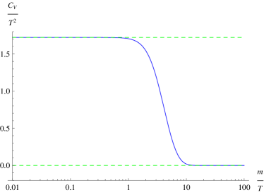
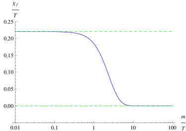
Figure 1: (a) The dependence of fermion specific heat on fermion gap $\frac{m}{T}$. The top dashed line corresponds to the non-interacting term $\mathcal{A}^{0f}_{C_{V}}=\frac{9\zeta(3)}{2\pi}$ at $m=0$. (b) The dependence of fermion susceptibility on fermion gap $\frac{m}{T}$. The top dashed line corresponds to the non-interacting term $\mathcal{A}^{0f}_{\chi_{f}}=\frac{\ln 2}{\pi}$ at $m=0$. It is obvious that fermion gap suppresses fermion specific heat and susceptibility strongly.

3.2 Interaction corrections

We now include the interaction correction to the free energy. Note the Goldstone bosons are neutral, so the Coulomb interaction only affects the free energy of Dirac fermions. To calculate the free energy $f^{1f}$, we should first know the polarization function. In the presence of finite fermion mass $m$ and external magnetic field $H$, the polarization function $\Pi(\omega_{m},\mathbf{q},T)$ can be calculated by the methods presented in [14, 27, 26]. Here we only write down the final expression:

$$\Pi(\omega_{m},\mathbf{q},T)$$

$$=\frac{NT}{\pi}\int_{0}^{1}dx\ln[4D_{m}]$$

$$\,\,-\frac{N}{4\pi}\int_{0}^{1}dx\frac{(1-2x)\omega_{m}\sin(\frac{1}{T}x\omega_{m}+\frac{1}{T}\theta H)}{D_{m}}$$

$$\,\,-\frac{N}{2\pi}\int_{0}^{1}dx\frac{m^{2}+x(1-x)\omega_{m}^{2}}{E_{f}}\frac{\sinh(\frac{1}{T}E_{f})}{D_{m}},$$ (27)

at finite temperature. Here we introduced the following abbreviated notations

$$E_{f} = \sqrt{m^{2}+x(1-x)(\mathbf{q}^{2}+\omega_{m}^{2})},$$ (28)

$$D_{m} = \cosh^{2}(\frac{E_{f}}{2T})-\sin^{2}(\frac{x\omega_{m}+\theta H}{2T}).$$ (29)

The zero-temperature limit of polarization function (Eq. (3.2)) is

$$\Pi(\omega_{m},\mathbf{q},T=0)=\frac{N}{\pi}\int_{0}^{1}dx\frac{x(1-x)\mathbf{q}^{2}}{E_{f}}.$$ (30)

Using Eq. (3.2) and Eq. (30), the free energy $f^{1f}$ (Eq. (15)) can be directly computed.

In the semimetal phase with $m=0$, the polarization function is

$$\Pi(\omega_{m},\mathbf{q},T,m=0)=\frac{\mathbf{q}^{2}}{\mathbf{q}^{2}+\omega_{m}^{2}}\frac{NT}{\pi}\int_{0}^{1}dx$$

$$\,\,\times\ln\left[2\left(\cosh(\frac{E_{f0}}{T})+\cos(\frac{x\omega_{m}}{T}+\theta\frac{H}{T})\right)\right],$$ (31)

at finite temperature with $E_{f0}=\sqrt{x(1-x)(\mathbf{q}^{2}+\omega_{m}^{2})}$ and

$$\Pi(\omega_{m},\mathbf{q},T=0,m=0)=\frac{N}{8}\frac{\mathbf{q}^{2}}{\sqrt{\mathbf{q}^{2}+\omega_{m}^{2}}},$$ (32)

at zero temperature. Using these expressions, the free energy of Dirac fermion is written as

$$f^{1f}=\frac{4T^{3}}{\pi^{3}}\int_{\delta}^{\frac{\Lambda}{T}}\!\mathbf{q}\,d\mathbf{q}\int_{0}^{\infty}dy\int_{0}^{1}dx\{K(x,y,\mathbf{q})+J(x,y,\mathbf{q})\},$$

where

$$K(x,y,\mathbf{q}) = \frac{\exp\left[-2\mathbf{q}\sqrt{x(1-x)(1+y^{2})}\right]}{\pi(1+y^{2})\left[\frac{1}{\lambda}+\frac{1}{\sqrt{1+y^{2}}}\right]},$$ (33)

$$J(x,y,\mathbf{q}) = \frac{2\exp\left[-\mathbf{q}\sqrt{x(1-x)(1+y^{2})}\right]}{\pi(1+y^{2})\left[\frac{1}{\lambda}+\frac{1}{\sqrt{1+y^{2}}}\right]}$$ (34)

$$\times\cos(xy\mathbf{q}+\theta\frac{H}{T}).$$

Here, a variable $y\equiv\frac{\omega}{\mathbf{q}}$ is introduced, with $\omega$ being the continuous form of $\omega_{m}$ when $T\rightarrow 0$. For finite $y$, $K(x,y,\mathbf{q})$ damps rapidly with growing $y$, so $y\sim 0$ makes the dominant contribution to the free energy. We can expand the function $K(x,y,\mathbf{q})$ near this point and obtain

$$f^{1f}_{1} = \frac{4T^{3}}{\pi^{3}}\int_{\delta}^{\frac{\Lambda}{T}}\mathbf{q}\,d\mathbf{q}\int_{0}^{\infty}dy\int_{0}^{1}dx\,K(x,y,\mathbf{q})$$ (35)

$$= \frac{8T^{3}}{\pi^{3}}\int_{\delta}^{\frac{\Lambda}{T}}\mathbf{q}\,d\mathbf{q}\int_{0}^{\infty}dy\int_{0}^{\frac{1}{2}}dx$$

$$\times\frac{\exp\left[-\mathbf{q}\sqrt{(1-4x^{2})(1+y^{2})}\right]}{(1+y^{2})\left[\frac{1}{\lambda}+\frac{1}{\sqrt{1+y^{2}}}\right]}$$

$$\approx \frac{8T^{3}}{\pi^{3}}\int_{\delta}^{\frac{\Lambda}{T}}\mathbf{q}\,d\mathbf{q}\int_{0}^{\infty}dy\frac{1}{(1+y^{2})\left[\frac{1}{\lambda}+\frac{1}{\sqrt{1+y^{2}}}\right]}$$

$$\times\int_{0}^{\frac{1}{2}}\frac{dx}{\exp\left[2\mathbf{q}\sqrt{x}\sqrt{(1+y^{2})}\right]}$$

$$= \frac{4}{\pi^{3}}\eta(\lambda)\,T^{3}\ln\frac{\Lambda}{T},$$

where

$$\eta(\lambda)=1+\frac{\tan^{-1}\left[\frac{\sqrt{1-\lambda^{2}}}{\lambda}\right]}{\lambda\sqrt{1-\lambda^{2}}}-\frac{\pi}{2\lambda}.$$ (36)

Comparing with $K(x,y,\mathbf{q})$, the form of $J(x,y,\mathbf{q})$ is more complicated owing to the cosine term $\cos(xy\mathbf{q}+\theta H/T)$. The computation becomes difficult if we make Taylor expansion of the cosine function. By plotting the dependence of function $J(x,y,\mathbf{q})$ on its variables, we found that the dominant regime is $x\sim 0,\,y\sim 0$. Hence, we simply take $J(x,y,\mathbf{q})$ as

$$J(x,y,\mathbf{q})\approx\frac{2\exp\left[-\mathbf{q}\sqrt{x(1+y^{2})}\right]}{(1+y^{2})\left[\frac{1}{\lambda}+\frac{1}{\sqrt{1+y^{2}}}\right]}\cos(\theta\frac{H}{T}),$$ (37)

which then leads to

$$f^{1f}_{2} = \frac{4T^{3}}{\pi^{3}}\int_{\delta}^{\frac{\Lambda}{T}}\mathbf{q}\,d\mathbf{q}\int_{0}^{\infty}dy\int_{0}^{1}dx\,J(x,y,\mathbf{q})$$ (38)

$$\approx \frac{16}{\pi^{3}}\eta(\lambda)\cos(\theta\frac{H}{T})\,T^{3}\ln\frac{\Lambda}{T}.$$

Taking $H=0$, the total free energy now has the form

$$f^{1f}=\frac{20}{\pi^{3}}\eta(\lambda)\,T^{3}\ln\frac{\Lambda}{T}.$$ (39)

It is easy to get the following specific heat and susceptibility

$$C_{V}^{1f} = -\frac{120}{\pi^{3}}\eta(\lambda)\,T^{2}\ln\frac{\Lambda}{T},$$ (40)

$$\chi_{f}^{1f} = -\frac{32}{\pi^{3}}\eta(\lambda)\,T\ln\frac{\Lambda}{T}.$$ (41)

Here, the ultraviolet cutoff $\Lambda$ can be taken to be of order $10$eV, which is determined by $\sim a^{-1}$ with lattice constant $a=2.46\textrm{\AA}$. From these results, we know that both specific heat and susceptibility of massless Dirac fermions exhibit logarithmic $T$-dependence due to long-range Coulomb interaction. These are non-Fermi liquid behaviors.

The appearance of such singular fermion specific heat was first pointed out by Vafek [7]. Here, we obtained the same qualitative $T$-dependence by a different method. In Ref. [7], the calculation of free energy was performed on the basis of the retarded vacuum polarization functions and retarded fermion propagator $G^{{\rm ret}}(\omega,\mathbf{k})=\frac{1}{\omega-\sigma\cdot\mathbf{k}}$, while in our case the polarization functions and fermion propagator are expressed in the Matsubara formalism. Strictly speaking, these two polarization functions are equivalent and should lead to the same results. We numerically compute the free energy using both the polarization functions obtained in the present paper and that in Ref. [7], and found that the results are very close to each other (the maximum proportional error of the coefficient $\frac{\delta f}{T^{3}\ln\frac{\Lambda}{T}}$ is $<5\%$). In order to get an analytic expression for free energy, some approximations to the polarization functions is unavoidable. In Ref. [7], the dominant contribution of polarization function comes from $y\equiv\frac{\omega}{{\bf q}}\sim 1$ at both $y>1$ and $y<1$ regions (after analytic continuation the momentum becomes $q=\sqrt{{\bf q}^{2}-(\omega+i\delta)^{2}}={\bf q}\sqrt{1-y^{2}}$), while in our calculation the dominant momentum region is $y\equiv\frac{\omega_{m}}{{\bf q}}\sim 0$ ($y\equiv\frac{\omega}{{\bf q}}\sim 0$ in the continuous form). For this reason, our analytic expression for the free energy differs from that of Ref. [7] (the approximation of $J(x,y,q)$ might partly explain the difference). After comparing the analytical results with numerical results, we found that our analytical result is slightly lower than the numerical result while the analytical result in Ref. [7] is slightly greater than the numerical result. For $\lambda=1$, the analytical and numerical results for the coefficient are $0.277$ and $0.231$ respectively in our work and $0.200$ and $0.225$ respectively in Ref. [7].

The contribution of Coulomb interaction to the free energy in the semimetal phase with $m=0$ is shown in Fig. 2. The free energy behaves as $\propto T^{3}\ln T$ (logarithmic correction) for several different values of $\lambda$.

We now turn to the insulator phase where $m\neq 0$. The free energy can be obtained by substituting Eq. (3.2) and Eq. (30) into Eq. (15). The dependencies of specific heat and susceptibility on different fermion mass $m$ for $\lambda=4$ are shown in Fig. 3 and 3, respectively. The results for other choices of $\lambda$ are similar and thus not shown. Here, we use the absolute values $|\mathcal{A}^{1f}_{C_{V}}|=-\mathcal{A}^{1f}_{C_{V}}$ and $|\mathcal{A}^{1f}_{\chi_{f}}|=-\mathcal{A}^{1f}_{\chi_{f}}$, instead of $\mathcal{A}^{1f}_{C_{V}}$ and $\mathcal{A}^{1f}_{\chi_{f}}$ which are negative. From Fig. 3 and 3, we see that the fermion gap leads to remarkable suppression of the interaction correction to fermion specific heat and susceptibility.

In summary, in the semimetal phase the long-range Coulomb interaction gives rise to non-Fermi liquid behavior of specific heat and susceptibility. In the insulator phase, the fermion specific heat and susceptibility are both significantly suppressed by the excitonic gap, but the total specific heat has a finite value due to the massless Goldstone bosons.

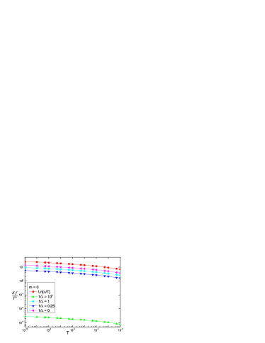
Figure 2: Interaction correction to free energy in the semimetal phase with $m=0$ for different interaction strength $\lambda$. The red line is the reference free energy $\ln\frac{\Lambda}{T}$. It appears that free energy displays the same logarithmic behavior for different $\lambda$.

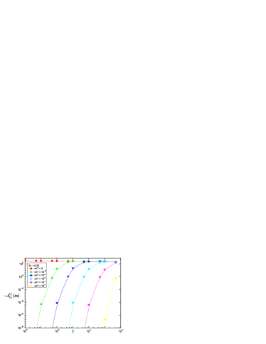
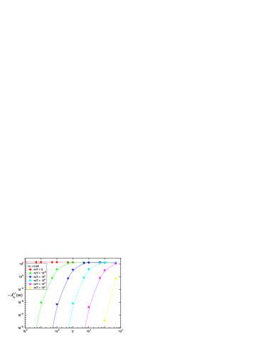
Figure 3: (a) Interaction correction to fermion specific heat in the insulator phase with $m\neq 0$ at $\lambda=4$. (b) Interaction correction to susceptibility in the insulator phase with $m\neq 0$ at $\lambda=4$. The suppressing effect of fermion gap is apparent.

4 Conclusion and discussion

In this paper, we calculated the specific heat and susceptibility in graphene. The ground state of graphene is semimetal when the Coulomb interaction strength $\lambda<\lambda_{c}$, but becomes insulator when $\lambda>\lambda_{c}$. The most prominent feature of semimetal phase is the appearance of logarithmic $T$-dependence of specific heat and susceptibility due to long-range Coulomb interaction. These are non-Fermi liquid behaviors. In the insulating phase, because the interaction correction to fermion excitations is strongly suppressed by the excitonic gap, the total specific heat is solely determined by the contribution from Goldstone bosons, while the susceptibility drops significantly. Apparently, both specific heat and susceptibility manifest quite different behaviors in the two sides of the critical point $\lambda_{c}$.

Note that the semimetal and insulator phases both contain massless excitations: massless Dirac fermion in the former and massless Goldstone boson in the latter. They have different statistics and exhibit completely different behaviors. For example, the massless Dirac fermions can transfer heat current and produce a universal thermal conductivity [28] at $T=0$, while the Goldstone bosons only contribute a $\propto T^{3}$ term, which vanishes rapidly as $T\rightarrow 0$. The massless Dirac fermions also gives rise to a universal electric conductivity [28], although the predicted electronic conductivity is at invariance with experimental result (the famous missing $\pi$). The Goldstone bosons do not contribute to electric conductivity since they are neutral.

We should point out that the Goldstone bosons are exactly massless only when the Lagrangian respects a continuous chiral symmetry. If the continuous chiral symmetry is explicitly broken by some contact four-fermion interaction, then the Goldstone bosons are no longer strictly massless. Instead, they have a small mass as the result of dynamical breaking of appropriate continuous chiral symmetry [29]. In this case, our discussion and calculation about the free energy contribution from Goldstone bosons should be modified and a small mass should be included. In reality, there are various four-fermion interactions in the graphene [30, 31]. If the contact four-fermion interaction has the form $\propto(\bar{\psi}\gamma_{0}\psi)^{2}$, then the continuous chiral symmetry is not explicitly broken and the Goldstone bosons are still massless. If the four-fermion interaction term is $\propto(\bar{\psi}\psi)^{2}$, then the system has only discrete chiral symmetry and there are no massless Goldstone bosons [14, 31]. Therefore, the specific heat of Goldstone bosons presented in Sec.3 is valid only when the continuous chiral symmetry is not explicitly broken by any four-fermion interaction term.

We finally comment on the validity of $1/N$ expansion. The excitonic insulating transition requires the Coulomb interaction between Dirac fermions be sufficiently strong. In this strong coupling regime, $1/N$ seems to be the only available expansion parameter, even if it is not small ($N=2$ for graphene). In our specific case, the fermion mass plays the dominant role in the insulator phase. It suppresses significantly the Coulomb interaction contribution to fermion specific heat. This implies that, within the $1/N$ expansion, the next-to-leading order contribution could be neglected since it is much less than the leading order contribution. It is reasonable to speculate that higher order corrections in $1/N$ expansion are also suppressed by the dynamical fermion mass. In the semimetal phase, there is no such suppressing effect, so higher order corrections might be important. As shown in the context, the analytical calculation of next-to-leading order correction is already very complicated, including higher order corrections will make analytical calculation intractable. The specific heat of massless Dirac fermions may be analyzed by renormalization group approach [6, 32], which found power-law $T^{\beta}$ behavior after summing up all orders of logarithmic corrections [6, 32]. However, the exponent $\beta$ can only be calculated by performing $1/N$ expansion. Therefore, the validity of $1/N$ expansion also needs to be studied in this approach.

5 Acknowledgments

We thank G. Cheng and J.-R. Wang for discussions. W. L. is grateful to R. Asgari for very helpful correspondence. This work is supported by National Science Foundation of China under Grant No. 10674122.

References

- [1] A. H. Castro Neto, F. Guinea, N. M. R. Peres, K. S. Novoselov, and A. K. Geim, Rev. Mod. Phys. 81 (2009) 109 .
- [2] J. Gonzalez, F. Guinea, and M. A. H. Vozmediano, Nucl. Phys. B 424 (1994) 595.
- [3] D. V. Khveshchenko, Phys. Rev. Lett. 87 (2001) 246802; D. V. Khveshchenko and H. Leal, Nucl. Phys. B 687 (2004) 323.
- [4] E. V. Gorbar, V. P. Gusynin, V. A. Miransky, and I. A. Shovkovy, Phys. Rev. B 66 (2002) 045108.
- [5] I. F. Herbut, Phys. Rev. Lett. 97 (2006) 146401.
- [6] D. T. Son, Phys. Rev. B 75 (2007) 235423.
- [7] O. Vafek, Phys. Rev. Lett. 98 (2007) 216407.
- [8] D. E. Sheehy and J. Schmalian, Phys. Rev. Lett. 99 (2007) 226803.
- [9] J. Gonzalez, F. Guinea, and M. A. H. Vozmediano, Phys. Rev. Lett. 77 (1996) 17.
- [10] S. Das Sarma, E. H. Hwang, and W. K. Tse, Phys. Rev. B 75 (2007) 121406.
- [11] D. V. Khveshchenko and W. F. Shively, Phys. Rev. B 73 (2006) 115104; D. V. Khveshchenko, J. Phys: Condens. Matter 21 (2009) 075303.
- [12] S. J. Hands and C. G. Strouthos, Phys. Rev. B 78 (2008) 165423.
- [13] J. E. Drut and T. A. Lahde, Phys. Rev. Lett. 102 (2009) 026802; Phys. Rev. B 79 (2009) 165425.
- [14] G.-Z. Liu, W. Li, and G. Cheng, Phys. Rev. B 79 (2009) 205429.
- [15] Y. Nambu and G. Jona-Lasinio, Phys. Rev. 122 (1961) 345.
- [16] T. Appelquist, D. Nash, and L. C. R. Wijewardhana, Phys. Rev. D 33 (1986) 3704.
- [17] T. Appelquist, D. Nash, and L. C. R. Wijewardhana, Phys. Rev. Lett. 60 (1988) 2575.
- [18] V. P. Gusynin, S. G. Sharapov, and J. P. Carbotte, Phys. Rev. Lett. 96 (2006) 256802; V. P. Gusynin and S. G. Sharapov, Phys. Rev. B. 73 (2006) 254511; V. P. Gusynin, V. A. Miransky, S. G. Sharapov, and I. A. Shovkovy, Phys. Rev. B. 74 (2006) 195429.
- [19] V. N. Kotov, B. Uchoa, and A. H. Castro Neto, Phys, Rev. B 80 (2009) 165424.
- [20] A. Qaiumzadeh and R. Asgari, New J. Phys. 11 (2009) 095023.
- [21] H. Jiang, G.-Z. Liu, and G. Cheng, Phys. Rev. B 79 (2009) 174503.
- [22] R. K. Kaul and S. Sachdev, Phys. Rev. B 77 (2008) 155105.
- [23] J. I. Kapusta and C. Gale, Finite-temperature field theory: principles and applications, (Cambridge, UK; New York,1994).
- [24] M. R. Ramezanali, M. M. Vazifeh, R. Asgari, M. Polini, and A. H. MacDonald, J. Phys. A: Math. Theor. 42 (2009) 214015.
- [25] A. V. Chubukov, D. L. Maslov, S. Gangadharaiah, and L. I. Glazman, Phys. Rev. B 71 (2005) 205112.
- [26] G.-Z. Liu, W. Li, and G. Cheng, Nucl. Phys. B 825 (2010) 303.
- [27] N. Dorey and N. E. Mavromatos, Nucl. Phys. B 386 (1992) 614.
- [28] P. A. Lee, Phys. Rev. Lett. 71, 1887 (1993); A. Durst and P. A. Lee, Phys. Rev. B 62, 1270 (2000).
- [29] S. Weinberg, The Quantum Theory of Fields, Vol. II, Chap.19 (Cambridge University Press, 1996).
- [30] J. Alicea and M. P. A. Fisher, Phys. Rev. B 74 (2006) 075422.
- [31] O. V. Gamayun, E. V. Gorbar, and V. P. Gusynin, arXiv:0911.4878v1.
- [32] C. Xu, Y. Qi and S. Sachdev, Phys. Rev. B 78 (2008) 134507.