Casimir-Polder interaction between an atom and a dielectric slab

Abstract

We present an explicit analytic calculation of the energy-level shift of an atom in front of a non-dispersive and non-dissipative dielectric slab. We work with the fully quantized electromagnetic field, taking retardation into account. We give the shift as a two-dimensional integral and use asymptotic analysis to find expressions for it in various retarded and non-retarded limiting cases. The results can be used to estimate the energy shift of an atom close to layered microstructures.

I Introduction

Control and manipulation of cold atoms have become fundamentally important due to their central role in the development of nanotechnology and as a tool for investigating the mechanisms underlying macroscopic manifestations of quantum physics Chan . It now seems feasible to control them on a $\mu$m length-scale by utilizing microstructured surfaces — also known as atoms chips — with promising areas of application such as quantum information processing with neutral atoms, integrated atom optics, precision force sensing, and studies of the interaction between atoms and surfaces.

For this reason, e.g., experiments using Bose-Einstein condensates for measuring the Casimir-Polder force CP have been developed. Typically, the dielectric substrate utilized in such experiments Obrecht carries a very thin top layer of another material, generally graphite or gold. However, in explicit analytic theories, this finite thickness has often been neglected and the system has been treated as a semi-infinite half-space. Here we are aiming at an approach that lets us include the thickness of such a layer as a parameter into the calculation, allowing us to obtain analytic expressions for the Casimir-Polder force on an atom.

We are going to consider a ground-state atom close to a non-dispersive dielectric slab, which is one of the fews systems of high symmetry for that the electromagnetic field can be quantized through an exact normal-mode expansion with manageable effort Khosravi . The assumption of absent dispersion and absorption is working well for all but very few systems, namely those where the atom has a strong transition very near an absorption line in the medium, which in practice is something very difficult to engineer. Nevertheless, if one wishes to consider more complex systems with atoms near absorbing boundaries, the calculation will require other methods to study quantum electrodynamics Abrikosov . However, applying such results to a particular case might require extensive numerical calculations for the case at hand. Using those types of formalism, the energy-level shift of atoms due to the presence of media with diverse magneto-electric properties has been calculated for several systems Buhmann . Here, by contrast, we are not aiming at general expressions. The focal point of the present work is to obtain simple and practical formulae that are useful for estimates and can be applied very easily to experimental situations.

The energy shift in an atom close to a dielectric slab comes about due to its interaction with electromagnetic field fluctuations, which in turn are affected by the presence of the slab. Thus, a quantization of the electromagnetic field in the presence of a layered system is required. Even though the field quantization for this system had been studied previously Khosravi , we have recently re-considered the problem and provided a proof of the completeness of the electromagnetic field modes that was missing in previous works on the problem. This proof of completeness is very useful in that it removes any ambiguity in how to normalize and sum over the electromagnetic field modes, and in this way also establishes the correct density of states which had previously been a subject of disagreement Zakowicz .

By solving the Helmholtz equation and imposing the corresponding continuity conditions at the faces of the slab, it was shown in Khosravi ; completeness that the field modes for this system comprise of travelling and trapped modes. The travelling modes have a continuous frequency spectrum, and are composed of incident, reflected and transmitted parts outside the slab. The trapped modes arise due to solutions of the Helmholtz equation with purely imaginary normal wave vector outside the slab. Physically, they come about due to repeated total internal reflection inside the dielectric, and emerge as evanescent fields outside the slab. They exist only at certain discrete frequencies which depend on polarization direction and parity and are obtained through the dispersion relations.

The atomic energy shift is obtained by means of second-order perturbation theory, and involves a product of electromagnetic mode functions which is summed over intermediate virtual photon states. Thus the atomic energy shift receives two quite separate contributions: one from the continuous set of travelling modes, and the other from the discrete set of trapped modes. The first is an integral over wave numbers, and the second a sum over discrete wave numbers that satisfy a quite complicated dispersion relation. In practice, both must be considered together at all times to avoid divergent terms appearing in each separate contribution but cancelling between them. This technically seemingly hopeless task can, however, be dealt with simply and elegantly by using the summation method of completeness , which re-expresses both the integral over continuous modes and the sum over discrete modes as a single contour integral in the complex plane. We shall show below that this trick yields a closed-form expression for the atomic energy shift and permits easy asymptotic analysis for various regimes, yielding the kinds of simple formulae that we are after for estimating the effect of the layer thickness in experimental situations.

II Description of the system

We consider a dielectric slab of finite thickness $L$ surrounded by vacuum, as is shown in Fig. 1. We assume the material to be a non-dispersive and non-absorbing dielectric, which is a simple but good model for an imperfectly reflecting material. Thus the material is characterized solely by its refractive index $n$, which is real and the same for all frequencies. While any real material has of course to be transparent at infinite frequencies, this non-dispersive model captures the essential properties of an imperfect reflector. In particular, it includes evanescent waves, whose absence in perfect-reflector models can be problematic robaschik .

Since the dielectric is homogeneous in the $x$ and $y$ directions, the dielectric permittivity of the configuration depends only on the $z$ coordinate and is given by

$$\varepsilon(z)=\left\{\begin{array}[]{ll}n^{2}&\qquad\textrm{for}\qquad-L/2\leq z\leq L/2\;,\\ 1&\qquad\textrm{for}\qquad|z|\geq L/2\;.\end{array}\right.$$

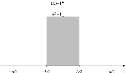
Figure 1: The geometry of the dielectric slab.

We assume the atom to be neutral and in its ground state. Also, we shall make use of the electric dipole approximation, which is adequate because, for the relevant modes, the electromagnetic field varies slowly over the size of the atom. We assume that the atom’s center is fixed at the position ${\bf r}_{0}=(0,0,z_{0})$.

The model assumes that the interaction between the atom and the surface is purely electromagnetic, i.e. that there is negligible wave-function overlap between the atomic electron and the surface.

We shall work with an interaction Hamiltonian between the atom and the quantized electromagnetic field that is given by

$$H_{\mbox{\footnotesize int}}=-\boldsymbol{\mu}\cdot{\bf E}({\bf r},t)\;,$$ (1)

which is the lowest-order multipole Hamiltonian and corresponds to the electric-dipole interaction. In this equation, $\boldsymbol{\mu}=e({\bf r}-{\bf r}_{0})$ is the electric-dipole moment of the atomic electron, and ${\bf E}({\bf r},t)$ is the transverse electric field. Unlike the minimal-coupling Hamiltonian ${\bf p}\cdot{\bf A}$, the Hamiltonian (1) includes the electrostatic interaction between the atomic dipole and its images on the other side of vacuum-dielectric interfaces. As shown previously in a similar context Eberlein , the Hamiltonian (1) may be more convenient for calculations that aim to derive energy shifts in cases where the retardation of the electromagnetic interaction matters.

The quantization of the electromagnetic field has been discussed in detail previously Khosravi ; completeness , and thus, we shall only sketch the procedure here. We work with the electromagnetic potentials $\Phi(\mathbf{r},t)$ and ${\bf A}(\mathbf{r},t)$ and choose the generalized Coulomb gauge

$${\nabla}\cdot\left[\varepsilon(z){\bf A}(\mathbf{r})\right]=0.$$ (2)

Furthermore, since the overall system is neutral, we can set $\Phi(\mathbf{r},t)=0$. Thus the field equations reduce to the wave equation for ${\bf A}(\mathbf{r},t)$ everywhere except right on the interfaces $z=\pm L/2$. At the interfaces we solve Maxwell’s equations directly by imposing the continuity conditions

$$E_{\|},\quad D_{\perp},\quad{\bf B}\qquad{\rm continuous}\;.$$ (3)

In this way the electromagnetic field modes can be written, for travelling modes $\mathbf{f}_{\nu}^{L,R}$ as left- or right-incident waves made up of incoming, reflected and transmitted parts, and for trapped modes $\mathbf{f}_{\nu}^{S,A}$, as symmetric or antisymmetric waves inside the slab with evanescent fields outside. We list these modes in Appendix A.

Equipped with a complete set of solutions to the classical field equations, we can proceed to quantize the electromagnetic field by using the technique of canonical quantization, i.e. by introducing annihilation and creation operators $a_{\nu}$, $a_{\nu}^{\dagger}$. Then the expansion for the electric field operator ${\bf E}(\mathbf{r},t)$ in terms of the normal modes $\mathbf{f}_{\nu}(\mathbf{r})$ reads

$${\bf E}(\mathbf{r},t)={\rm i}\sum_{\nu}\sqrt{\frac{\omega_{\nu}}{2\varepsilon_{0}}}\left[a_{\nu}e^{-{\rm i}\omega_{\nu}t}\mathbf{f}_{\nu}(\mathbf{r})-a_{\nu}^{\dagger}e^{{\rm i}\omega_{\nu}t}\mathbf{f}_{\nu}^{*}(\mathbf{r})\right].$$ (4)

where the subscript $\nu=(\mathbf{k},\lambda)$ is a composite label including both the polarization $\lambda=\mbox{TE},\mbox{TM}$ and the wave vector $\mathbf{k}$.

III Energy-level shift

Since the interaction Hamiltonian (1) is linear in the electric field, whose vacuum expectation value vanishes, there is no energy shift to first order in $H_{\mbox{\footnotesize int}}$. Therefore, the lowest-order contribution to the shift comes from second-order perturbation theory, so that the shift is of first order in the fine-structure constant $\alpha$ fn1 ,

$$\Delta E=-\sum_{j\neq i}\sum_{\nu}\frac{\left|\left\langle j;\nu|\boldsymbol{\mu}\cdot{\bf\hat{E}}(\mathbf{r},t)|i;0\right\rangle\right|^{2}}{E_{j}-E_{i}+\omega_{\nu}},$$ (5)

where ${\bf{\hat{E}}}({\bf r},t)$ is given by Eq. (4). In this equation, the intermediate state $\left|j;\nu\right\rangle$ is a composite state with an atom in the excited state $|j\rangle$ and the electromagnetic field carrying a photon of energy $\omega_{\nu}$. Similarly, the initial state $|i;0\rangle$ describes an atom in its ground state $|i\rangle$ and the electromagnetic field in the vacuum state. In the electric dipole approximation we can write

$$\left\langle j|\mathbf{f}(\mathbf{r})\cdot\boldsymbol{\mu}|i\right\rangle\simeq\mathbf{f}(\mathbf{r}_{0})\cdot\left\langle j|\boldsymbol{\mu}|i\right\rangle,$$ (6)

since the field varies slowly over the size of the atom and we can therefore assume that across the atom it is almost the same as at its center ${\bf r}_{0}=(0,0,z_{0})$. With this, the shift reads

$$\Delta E=-\frac{1}{2\varepsilon_{0}}\sum_{j\neq i}\sum_{\nu}\frac{\omega_{\nu}}{E_{ji}+\omega_{\nu}}\left|\mathbf{f}^{*}_{\nu}(\mathbf{r}_{0})\cdot\langle j|\boldsymbol{\mu}|i\rangle\right|^{2},$$ (7)

where we have introduced the abbreviation $E_{ji}=E_{j}-E_{i}$. Since $|i\rangle$ is a state of definite angular momentum, different components of $\boldsymbol{\mu}$ lead to different intermediate states $|j\rangle$ that are mutually orthogonal, and the shift simplifies to

$$\Delta E=-\frac{1}{2\varepsilon_{0}}\sum_{j\neq i}\sum_{\nu}\frac{\omega_{\nu}}{E_{ji}+\omega_{\nu}}\left|\mathbf{f}^{*}_{\nu}(\mathbf{r}_{0})|^{2}\;|\langle j|\boldsymbol{\mu}|i\rangle\right|^{2}.$$ (8)

Furthermore, we are going to abbreviate the moduli squares of the matrix elements of the dipole-momentum operator $\boldsymbol{\mu}$ between the initial state $i$ and the intermediate states $j$, and distinguish only the components parallel and perpendicular to the slab,

$$|\mu_{\sigma}|^{2}\equiv\left|\left\langle j|\mu_{\sigma}|i\right\rangle\right|^{2}\quad{\rm with}\quad\sigma=x,y,z$$

$$|\boldsymbol{\mu}_{||}|^{2}\equiv|\langle j|\mu_{x}|i\rangle|^{2}+|\langle j|\mu_{y}|i\rangle|^{2}$$

$$|\boldsymbol{\mu}_{\perp}|^{2}\equiv|\langle j|\mu_{z}|i\rangle|^{2}\;.$$

The sum over $\nu$ in Eq. (8) is a sum over all field modes, which, as explained earlier and easily seen from Appendix A, comprise a continuous set of travelling modes and a discrete set of trapped modes. The contribution from the travelling modes gives rise to the shift

$$\Delta E^{{\rm trav}}=-\frac{1}{2\varepsilon_{0}}\sum_{j\neq i}\sum_{\lambda=TE,TM}\sum_{\sigma}\int\mathrm{d}^{3}{\bf k}\frac{\omega}{E_{ji}+\omega}$$

$$\times\left(|{\bf f}^{L}_{\mathbf{k}\lambda\sigma}({\bf r}_{0})|^{2}+|{\bf f}^{R}_{\mathbf{k}\lambda\sigma}({\bf r}_{0})|^{2}\right)\left|\mu_{\sigma}\right|^{2},$$ (9)

where the sum over $\sigma$ runs over the $x$, $y$ and $z$ components of the dipole moment and of the polarization vector that is incorporated in the mode functions. As we are interested in the change in the energy levels of the atom solely due to the presence of the dielectric slab, we renormalize the energy shift and remove from Eq. (9) the part that arises due to the interaction between the atom and the electromagnetic field in free space, i.e. the Lamb shift. Conveniently, this rids the calculation of any divergences, provided travelling and trapped modes are considered together (cf. e.g. Wu-paper1 ). The simplest way to implement this renormalization of the shift is by subtracting the equivalent expression for a transparent slab with $n=1$,

$$\delta E^{{\rm trav}}\equiv\Delta E^{{\rm trav}}-\Delta E^{{\rm trav}}(n=1)\;.$$ (10)

We decide to place the atom at a position $z_{0}>L/2$ to the right of the slab, substitute the mode functions (49,53), and get

$$\delta E^{{\rm trav}}=-\frac{1}{2(2\pi)^{3}\varepsilon_{0}}\sum_{j\neq i}\sum_{\lambda,\,\sigma}\;\int\mathrm{d}^{3}\mathbf{k}\;\frac{\omega}{E_{ji}+\omega}\left|\mu_{\sigma}\right|^{2}$$

$$\times\;\hat{e}_{\lambda}^{\sigma}(\mathbf{k}^{+})\hat{e}_{\lambda}^{\sigma*}(\mathbf{k}^{-})\Big{(}R_{\lambda}\;e^{2{\rm i}k_{z}{z_{0}}}+R_{\lambda}^{*}\;e^{-2{\rm i}k_{z}{z_{0}}}\Big{)}.$$ (11)

Similarly, the contribution from the discrete set of trapped modes reads

$$\Delta E^{{\rm trap}}=-\frac{1}{2\varepsilon_{0}}\sum_{j\neq i}\sum_{\lambda,\,\sigma}\sum_{k_{z}}\int\mathrm{d}^{2}\mathbf{k}_{\parallel}\;\frac{\omega}{E_{ji}+\omega}$$

$$\times\;\left(|\mathbf{f}^{S}_{\mathbf{k}\lambda\sigma}(\mathbf{r}_{0})|^{2}+|\mathbf{f}^{A}_{\mathbf{k}\lambda\sigma}({\bf r}_{0})|^{2}\right)\left|\mu_{\sigma}\right|^{2},$$ (12)

which can be written in a more explicit form by substituting the trapped modes to the right of the slab from Eq. (54),

$$\delta E^{{\rm trap}}=-\frac{1}{2\varepsilon_{0}}\sum_{j\neq i}\sum_{\lambda,\,\sigma}\sum_{k_{z}}\int\mathrm{d}^{2}\mathbf{k}_{\parallel}\;\frac{\omega}{E_{ji}+\omega}\left|\mu_{\sigma}\right|^{2}$$

$$\times\;\hat{e}_{\lambda}^{\sigma}(\mathbf{k}^{+})\hat{e}_{\lambda}^{\sigma*}(\mathbf{k}^{-})\left|M_{\lambda}\right|^{2}\left|L_{\lambda}^{S,A}\right|^{2}e^{-2\kappa{z_{0}}}.$$ (13)

We note that renormalization makes no difference to the trapped-modes contribution to the shift, as the trapped modes vanish in the limit $n\rightarrow 1$.

The total energy shift is obtained by combining the travelling-mode contribution Eqs. (III) and the trapped-mode contribution (III). At first sight, this is very complicated, since the former is given by an integral over $k_{z}$ while the latter involves a sum over discrete values of $k_{z}={\rm i}\kappa$ that are solutions of the dispersion relations (61). In addition, the shift (III) due to travelling modes and its counterpart (III) due to trapped modes diverge when evaluated each on their own, as observed before in similar circumstances Wu-paper1 . What helps, is the observation that the reflection coefficients $R_{\lambda}$ have poles in the complex $k_{z}$ plane at exactly the values of $k_{z}={\rm i}\kappa$ that are solutions of the dispersion relations (61). Furthermore, the residues around those poles are such that the sum over $k_{z}$ in Eq. (III) can be re-written as a contour integral with the same integrand as in Eq. (III). Thus the sum of Eqs. (III) and (III) can be combined into a single contour integral in the complex $k_{z}$ plane. In Ref. completeness we have shown this to be the case in connection with a proof of the completeness of the electromagnetic field modes around a dielectric slab, and we refer the reader there for details. Using this method to add Eqs. (III) and (III), we obtain for the total energy shift

$$\delta E=-\frac{1}{2(2\pi)^{3}\varepsilon_{0}}\sum_{j\neq i}\sum_{\lambda,\sigma}\;\int\mathrm{d}^{2}\mathbf{k}_{\|}\int_{\mathcal{C}}\mathrm{d}k_{z}\;\frac{\omega}{E_{ji}+\omega}$$

$$\times\left|\mu_{\sigma}\right|^{2}\hat{e}_{\lambda}^{\sigma}(\mathbf{k}^{+})\hat{e}_{\lambda}^{\sigma*}(\mathbf{k}^{-})R_{\lambda}(k_{z},\mathbf{k}_{\parallel})\;e^{2{\rm i}k_{z}{z_{0}}}\;,$$ (14)

with the integration path $\mathcal{C}$ as shown in Fig. 2. The poles of $R_{\lambda}$ lie on the imaginary axis between 0 and ${\rm i}\sqrt{n^{2}-1}k_{\|}/n$, so that $\mathcal{C}$ runs above them.

Figure 2: By closing the contour $\mathcal{C}$ one can choose a more suitable integration path $\mathcal{C}^{\prime}$. In the figure, $\Gamma=\sqrt{n^{2}-1}/n$.

To manipulate this expression further, we sum over the two polarizations and re-arrange the Cartesian components $\sigma=x,y,z$ into parallel and perpendicular parts relative to the surface of the slab. The double integral in $\mathbf{k}_{\|}$ can be simplified by transforming into polar coordinates and carrying out the integration in the azimuthal angle, so that the total energy shift reads

$$\delta E=-\frac{1}{2\pi^{2}\varepsilon_{0}}\sum_{j\neq i}\sum_{\sigma=\|,\perp}\;E_{ji}^{3}\;S_{\sigma}\left|\boldsymbol{\mu}_{\sigma}\right|^{2}$$ (15)

with parallel and perpendicular contributions given, respectively, by

$$S_{\|}\equiv\frac{1}{8E_{ji}^{3}}\int_{0}^{\infty}\mathrm{d}k_{\|}\;k_{\|}I_{\|}\quad{\rm and}\quad S_{\perp}\equiv\frac{1}{4E_{ji}^{3}}\int_{0}^{\infty}\mathrm{d}k_{\|}\;k_{\|}I_{\perp}$$ (16)

and, in turn,

$$I_{\|}=\int_{\mathcal{C}}\mathrm{d}k_{z}\frac{\omega}{E_{ji}+\omega}\;R_{TE}(k_{z},\mathbf{k}_{\parallel})\ e^{2{\rm i}k_{z}{z_{0}}}$$

$$-\int_{\mathcal{C}}\mathrm{d}k_{z}\frac{\omega}{E_{ji}+\omega}\;\frac{k_{z}^{2}}{k^{2}}\;R_{TM}(k_{z},k_{\|})\;e^{2{\rm i}k_{z}{z_{0}}},$$ (17)

$$I_{\perp}=\int_{\mathcal{C}}\mathrm{d}k_{z}\frac{\omega}{E_{ji}+\omega}\;\frac{k_{\|}^{2}}{k^{2}}\;R_{TM}(k_{z},k_{\|})\ e^{2{\rm i}k_{z}{z_{0}}}.$$ (18)

Before proceeding with the evaluation of Eqs. (17) and (18), we note that both of them are written in terms of the position $z_{0}$ of the atom, measured from the center of the slab. In practice, one would of course want to know the energy shift of the atom as a function of its distance to the surface of the slab, $\mathcal{Z}=z_{0}-L/2$. Writing Eqs. (17) and (18) in terms of the atom-surface distance $\mathcal{Z}$ gives rise to a phase factor $e^{{\rm i}k_{z}L}$ which we absorb in the reflection coefficients (50) by redefining

$$\widetilde{R}_{\lambda}=r_{\lambda}\frac{1-e^{2ik_{\rm zd}L}}{1-r_{\lambda}^{2}e^{2ik_{\rm zd}L}}\;,$$ (19)

so that Eq. (18) turns into

$$I_{\perp}=\int_{\mathcal{C}}\mathrm{d}k_{z}\frac{\omega}{E_{ji}+\omega}\;\;\frac{k_{\|}^{2}}{k^{2}}\;\widetilde{R}_{TM}\;e^{2{\rm i}k_{z}{\cal Z}},$$ (20)

and similarly for Eq. (17). Since the photon frequency is given by $\omega=\sqrt{k_{\|}^{2}+k_{z}^{2}}$, one can identify branch points in the integrand at $k_{z}=\pm{\rm i}k_{\|}$. We choose to place the square-root cuts from $k_{z}={\rm i}k_{\|}$ to ${\rm i}\infty$ and from $k_{z}=-{\rm i}k_{\|}$ to $-{\rm i}\infty$. Apart from this square-root cut, the integrand is analytic in the upper half-plane and for $\mathcal{Z}>0$ vanishes exponentially on the infinite semicircle in the upper half-plane. Therefore Cauchy’s theorem allows us to deform the original integration path $\mathcal{C}$ into a new path $\mathcal{C}^{\prime}$ that goes round the square-root cut from ${\rm i}k_{\|}$ to ${\rm i}\infty$ (see Fig. 2). Identifying the correct sheet on each side of the cut by demanding that $\omega>0$ on the real $k_{z}$ axis and re-expressing $k_{z}={\rm i}q$, we can work out the integral along the path $\mathcal{C}^{\prime}$ and obtain

$$I_{\perp}=2E_{ji}\int_{k_{\|}}^{\infty}\mathrm{d}q\;\frac{k_{\|}^{2}}{\sqrt{q^{2}-k_{\|}^{2}}}\;\frac{\widetilde{R}_{TM}}{E_{ji}^{2}-k_{\|}^{2}+q^{2}}\;e^{-2q{\cal Z}}.$$ (21)

The calculation of the parallel contribution $I_{\parallel}$, Eq. (17), runs along exactly the same lines. Substituting Eq. (21) into Eq. (16), we see that the two contributions $S_{\|}$ and $S_{\perp}$ to the energy shift (15) are both double integrals, over $k_{\|}$ and over $q=-{\rm i}k_{z}$. We choose to make a change of variables to $u=(q^{2}-k_{\|}^{2})^{1/2}/E_{ji}$ and $v=k_{\|}/E_{ji}$, and arrive at

$$S_{\|}\!\! = \!\!\frac{1}{4}\int_{0}^{\infty}\!\!\mathrm{d}v\int_{0}^{\infty}\!\!\mathrm{d}u\;\frac{v}{\sqrt{u^{2}+v^{2}}}\frac{1}{1+u^{2}}$$

$$\times\left[(u^{2}+v^{2})\widetilde{R}_{TM}-u^{2}\widetilde{R}_{TE}\right]\;e^{-2\mathcal{Z}E_{ji}\sqrt{u^{2}+v^{2}}},$$

and

$$S_{\perp}\!\! = \!\!\frac{1}{2}\int_{0}^{\infty}\!\!\mathrm{d}v\int_{0}^{\infty}\!\!\mathrm{d}u\;\frac{v^{3}}{\sqrt{u^{2}+v^{2}}}\;\frac{1}{1+u^{2}}\;\widetilde{R}_{TM}$$ (23)

$$\times\ e^{-2\mathcal{Z}E_{ji}\sqrt{u^{2}+v^{2}}}.$$

These expressions, together with Eq. (15), give us a general formula for the energy shift of a ground-state atom in front of a dielectric slab. The shift depends on the matrix elements of the atomic dipole between the initial state $|i\rangle$ and other states $|j\rangle$ that are coupled to $|i\rangle$ by strong dipole transitions. In practice, the sum in Eq. (15) over intermediate states $|j\rangle$ is in most cases dominated by a single close-lying state with a strong dipole transition to the initial atomic state $|i\rangle$. Alternatively, we can use the identity

$$\left|\langle j|\boldsymbol{\mu}_{\sigma}\right|i\rangle|^{2}=\frac{4\pi\varepsilon_{0}\alpha}{m^{2}E_{ji}^{2}}\left|\langle j|{\bf p}_{\sigma}|i\rangle\right|^{2},$$ (24)

where $\alpha=e^{2}/4\pi\varepsilon_{0}$ is the fine structure constant, and re-write the energy shift in terms of the matrix elements of the momentum operator,

$$\delta E=-\frac{2\alpha}{\pi m^{2}}\sum_{j}\sum_{\sigma=\|,\perp}\;E_{ji}S_{\sigma}|p_{\sigma}|^{2}\;.$$ (25)

In this form the shift is very similar to that of an atom in front of a dielectric half-space (cf. Eqs. (2.12), (2.25), and (2.26) of Ref. Eberlein ), except for the different reflection coefficients in each situation.

In order to further analyse or calculate the energy shift numerically, it is convenient to transform the double integrals in Eqs. (III) and (23) into polar coordinates by substituting $u=s\cos\phi$ and $v=s\sin\phi$, and then replace $\phi$ by $t=\cos\phi$. This gives

$$S_{\|}=\frac{1}{4}\int_{0}^{\infty}\mathrm{d}s\int_{0}^{1}\mathrm{d}t\;\frac{s^{3}}{s^{2}t^{2}+1}\;\left(\widetilde{R}_{TM}-t^{2}\widetilde{R}_{TE}\right)\;e^{-2\mathcal{Z}E_{ji}s},$$ (26)

$$S_{\perp}=\frac{1}{2}\int_{0}^{\infty}\mathrm{d}s\int_{0}^{1}\mathrm{d}t\;\frac{s^{3}}{s^{2}t^{2}+1}\;\left(1-t^{2}\right)\widetilde{R}_{TM}\;e^{-2\mathcal{Z}E_{ji}s},$$ (27)

with reflection coefficients

$$\widetilde{R}_{TE}=\frac{-(n^{2}-1)t^{2}}{2+(n^{2}-1)t^{2}+2\sqrt{1+(n^{2}-1)t^{2}}\coth\Lambda}$$ (28)

$$\widetilde{R}_{TM}=\frac{n^{4}-1-(n^{2}-1)t^{2}}{n^{4}+1+(n^{2}-1)t^{2}+2n^{2}\sqrt{1+(n^{2}-1)t^{2}}\coth\Lambda}$$ (29)

and the abbreviation $\Lambda=LE_{ji}s\sqrt{1+(n^{2}-1)t^{2}})$. Thus the energy shift of the atom in front of a dielectric slab is given by Eqs. (15) or (25), with Eqs. (26)–(29). In this form the shift is readily computed numerically, as we shall do in Section V. However, to extract important physics and be in the position to make quick estimates, one should investigate the asymptotic behaviour of the shift in various physically significant regimes, which we shall do first.

IV Asymptotic analysis

The nature of the interaction of the atom with the slab depends on the separation between them: for large separations the interaction is manifestly retarded, but for small separations the retardation can be neglected and the interaction can be assumed to take place instantaneously. The scale on which one makes this distinction of the atom-surface separation being small or large, comes from comparing the time $2\mathcal{Z}/c$ that a virtual photon takes for a round-trip between atom and surface to the time scale of internal evolution of the atom. For the atom in state $|i\rangle$ with a strong dipole transition into a close-lying state $|j\rangle$, the time scale of the atom’s internal dynamics is given by $\hbar/E_{ji}$. The ratio of the two time scales is $2\mathcal{Z}E_{ji}$ in natural units, which can therefore be used as the criterion for retardation: the interaction is manifestly retarded for $2\mathcal{Z}E_{ji}\gg 1$, as the atom has evolved appreciably by the time the virtual photon has completed its round-trip, and it can be considered non-retarded for $2\mathcal{Z}E_{ji}\ll 1$, because the atomic state hardly changes while the photon travels to the surface and back. In terms of length scales, it is the relative sizes of the distance $\mathcal{Z}$ of the atom from the surface and the wavelength $1/E_{ji}$ of the strongest internal transition that matter. However, the thickness of the slab $L$ provides a third length scale to consider. We shall now consider the various asymptotics limits.

IV.1 Thick slab $L\gg\mathcal{Z}$

For a very thick slab, i.e. in the limit $L\rightarrow\infty$, we can approximate $\coth\Lambda\simeq 1$ in Eqs. (28) and (29). Then expressions (26) and (27) reduce to what they would be for a dielectric half-space Eberlein . The energy shift for an atom in front of a dielectric half-space has been analysed in detail previously in both the retarded and the non-retarded limits Wu-paper1 .

IV.2 Thin slab $L\ll\mathcal{Z}$

If the atom-surface separation $\mathcal{Z}$ is much larger than the slab thickness $L$ then the exponentials in Eqs. (26) and (27) effectively cut off the integral at very small values of $s$, so that the argument of the $\coth$ in Eqs. (28) and (29) stays very small throughout the whole effective range of integration. Thus we can approximate the $\coth$ by its small-argument expansion, $\coth\Lambda\simeq 1/\Lambda$. This leads to significant simplifications in Eqs. (28) and (29) because the square roots in the denominators drop out, and we get:

$$\widetilde{R}_{TE}\simeq\frac{-(n^{2}-1)t^{2}}{2+(n^{2}-1)t^{2}+2/(sLE_{ji})}$$ (30)

$$\widetilde{R}_{TM}\simeq\frac{n^{4}-1-(n^{2}-1)t^{2}}{n^{4}+1+(n^{2}-1)t^{2}+2n^{2}/(sLE_{ji})}\;.$$ (31)

Substituting these into Eqs. (26) and (27), we can now carry out the $t$ integral. While elementary, this integration gives an unwieldy combination of rational functions, square roots, and $\arctan$, so that we dispense with writing it down. The subsequent integration over $s$ cannot be performed analytically, unless we make further approximations, which we shall do in the following for the retarded and non-retarded limits.

IV.3 Retarded regime ($2\mathcal{Z}E_{ji}\gg 1$) for a “thin” slab

If $2\mathcal{Z}E_{ji}\gg 1$ then we can apply Watson’s lemma to the $s$ integrals in Eqs. (26) and (27). So, we substitute the approximated reflection coefficients (30) and (31), carry out the $t$ integration, and then expand the integrand of the $s$ integral around $s=0$, after which the $s$ integral over the leading term becomes elementary. In such a way we find that the energy-level shift is given by

$$\delta E\simeq-\frac{(n^{2}-1)L}{160\pi^{2}\varepsilon_{0}n^{2}\mathcal{Z}^{5}}\sum_{j\neq i}\;\frac{(5+9n^{2})|\mu_{\|}|^{2}+2(4+5n^{2})|\mu_{\perp}|^{2}}{E_{ji}}.$$ (32)

We would like to note that this result is valid for $2\mathcal{Z}E_{ji}\gg 1$ and $\mathcal{Z}\gg L$, but other than that for any slab thickness $L$. In particular, there is no restriction on $LE_{ji}$, which can have any size $>$ or $<1$ provided it is much smaller than $\mathcal{Z}E_{ji}$. In this sense the notion of a “thin” slab is slightly misleading in the retarded regime, as any slab of finite thickness can be considered thin for large enough $\mathcal{Z}$.

Another interesting aspect of this result is that it shows that there is absolutely nothing unusual or non-analytic about the limit $L\rightarrow 0$. A calculation of the Casimir-Polder force using field-theoretical means and four photon polarizations in a Gupta-Bleuler quantization scheme Bordag-sheet has found different results for different ways of implementing the boundary conditions on the photon field, and the tentative explanation for this discrepancy, as given in Ref. Bordag-sheet , has been that these different results should apply to thick and thin slabs. However, this explanation is inconsistent with our explicit results for the Casimir-Polder energy shift for slabs of arbitrary finite thickness.

IV.4 Non-retarded regime ($2\mathcal{Z}E_{ji}\ll 1$)

In the non-retarded limit the interactions between the atom and the slab can be approximated as instantaneous, and the energy shift in this regime can be calculated by considering the limit $E_{ji}\rightarrow 0$. One could take this limit in Eqs. (26)–(29), with Eqs. (15) or (25), but the calculation is much shorter if instead we go back to Eqs. (16)–(18), which was before we had deformed the contour $\mathcal{C}$ in the complex $k_{z}$ plane. In the limit $E_{ji}\rightarrow 0$, we get $\omega/(E_{ji}+\omega)\rightarrow 1$ in Eqs. (17) and (18), so that the square root cut due to $\omega=\sqrt{k_{\|}^{2}+k_{z}^{2}}$ disappears from them. Instead, we get poles at $k_{z}=\pm{\rm i}k_{\|}$. When we close the contour $\mathcal{C}$ in the upper half-plane, we pick up the residues of the integrands at $k_{z}={\rm i}k_{\|}$, so that Eqs. (17) and (18) turn into

$$I_{\|} = -\left.2\pi{\rm i}\;\mbox{Res}\frac{k_{z}^{2}\;\widetilde{R}_{TM}(k_{z},k_{\|})}{(k_{z}-{\rm i}k_{\|})(k_{z}+{\rm i}k_{\|})}\;e^{2{\rm i}k_{z}{\mathcal{Z}}}\right|_{k_{z}={\rm i}k_{\|}}$$ (33)

$$I_{\perp} = \left.2\pi{\rm i}\;\mbox{Res}\frac{k_{\|}^{2}\;\widetilde{R}_{TM}(k_{z},k_{\|})}{(k_{z}-{\rm i}k_{\|})(k_{z}+{\rm i}k_{\|})}\;e^{2{\rm i}k_{z}{\mathcal{Z}}}\right|_{k_{z}={\rm i}k_{\|}}\;,$$ (34)

which are straightforward to determine. Substituting the results into Eqs. (16) and (15), we obtain for the energy shift in the non-retarded regime

$$\Delta E_{{\rm es}}=-\frac{1}{16\pi\varepsilon_{0}}\;\frac{n^{2}-1}{n^{2}+1}\sum_{j\neq i}\left(2|\mu_{\perp}|^{2}+|\mu_{\|}|^{2}\right)$$

$$\times\int_{0}^{\infty}\mathrm{d}k\;k^{2}\;e^{-2\mathcal{Z}k}\frac{1-e^{-2kL}}{1-\left(\frac{n^{2}-1}{n^{2}+1}\right)^{2}e^{-2kL}}.$$ (35)

The same result could be achieved from purely electrostatic considerations. The atom can be viewed as a dipole, and the dielectric slab can be modelled as a series of image dipoles. The energy shift is then just the Coulomb interaction energy of the atomic dipole and its images. We show in Appendix B that an electrostatic calculation of this sort indeed reproduces the energy shift (35).

Finally we consider the limit $L\ll\mathcal{Z}$ and obtain for the non-retarded energy shift of an atom near a thin slab

$$\Delta E_{{\rm es}}\simeq-\frac{3(n^{4}-1)}{256\pi\varepsilon_{0}n^{2}}\frac{L}{\mathcal{Z}^{4}}\sum_{j\neq i}\left(2|\mu_{\perp}|^{2}+|\mu_{\|}|^{2}\right)\;.$$ (36)

V Summary and conclusions

We have obtained a general formula for the energy-level shift in a ground-state atom near a non-dispersive dielectric slab of refractive index $n$: Eq. (15), or alternatively Eq. (25), with the parallel and perpendicular contributions $S_{\|}$ and $S_{\perp}$ given by (26) and (27), respectively. While given only as a double integral, it is nevertheless in a form that is readily amenable to both numerical calculations and analytic approximations. We have given appropriate asymptotic formulae in both the retarded ($2\mathcal{Z}E_{ji}\gg 1$) and the non-retarded regimes ($2\mathcal{Z}E_{ji}\ll 1$). For the latter we showed that the result can be reproduced by means of a classical electrostatic treatment. For thin slabs the electrostatic energy shift varies as $L/\mathcal{Z}^{4}$, as shown in Eq. (36).

In the retarded regime, on the other hand, our general formula reduces to Eq. (32), showing that the shift behaves as $L/\mathcal{Z}^{5}$, provided $L\ll\mathcal{Z}$. For this case, it is possible to compare our result with the one given in Eq. (218) of Ref. Buhmann for the interaction energy between a ground-state atom and a magnetodielectric plate,

$$U(\mathcal{Z})=-\frac{\hbar c\alpha(0)}{160\pi^{2}\varepsilon_{0}}\frac{L}{\mathcal{Z}^{5}}\left[\frac{14\varepsilon^{2}(0)-9}{\varepsilon(0)}-\frac{6\mu^{2}(0)-1}{\mu(0)}\right],$$ (37)

where $\alpha(0)$ is the static polarizability of the atom. In order to compare this result to our result (32), we need to substitute $\varepsilon(0)=n^{2}$ for the static dielectric constant and $\mu(0)=1$ for the static magnetic permeability. Furthermore, the diagonal elements of the atomic polarizability are

$$\alpha_{\nu\nu}(\omega)=\sum_{j}\frac{2E_{ji}\left|\langle j|\mu_{\nu}|i\rangle\right|^{2}}{E_{ji}^{2}-\omega^{2}}\;,\quad\nu=\{x,y,z\}\;,$$ (38)

so that we get for the static polarizability of the isotropic atom considered in Ref. Buhmann

$$\alpha(0)=2\sum_{j\neq i}\frac{|\mu_{\nu}|^{2}}{E_{ji}}\;,\quad\nu=\{x,y,z\}\;.$$ (39)

In this language our expression (32) reads

$$\delta E=-\frac{\alpha(0)}{160\pi^{2}n^{2}\varepsilon_{0}}\frac{L}{\mathcal{Z}^{5}}(n^{2}-1)(9+14n^{2}),$$ (40)

which agrees with Eq. (37) upon substitution of $\varepsilon(0)=n^{2}$ and $\mu(0)=1$.

The great advantage of our general formulae (15), (26) and (27) is that they make it possible to know how the energy shift behaves for various slab thicknesses and values of the atom-surface separation $\mathcal{Z}$. Using these formulae and standard software packages such as Mathematica or Maple, one can easily plot $\delta E$ for any desired parameter ranges. In order to plot some examples in a meaningful and informative way, we re-write the energy shift in the following form

$$\delta E=-\frac{1}{4\pi\varepsilon_{0}}\sum_{j\neq i}\;\frac{1}{4\pi E_{ji}\mathcal{Z}^{4}}\left(W_{\|}^{\rm slab}|\mu_{\|}|^{2}+W_{z}^{\rm slab}|\mu_{z}|^{2}\right),$$ (41)

with parallel part and perpendicular contributions defined by

$$W_{\|}^{\rm slab}=64{\mathcal{Z}}^{4}E_{ji}^{4}S_{\|}\quad{\rm and}\quad W_{z}^{\rm slab}=64{\mathcal{Z}}^{4}E_{ji}^{4}S_{\perp},$$ (42)

and the functions $S_{\|,\perp}$ given as before in Eqs. (26) and (27). The motivation for this choice is that (i) $W_{\|}$ and $W_{\perp}$ are dimensionless quantities, and (ii) they facilitate easy comparison to the standard Casimir-Polder result CP as $W_{\|}=1=W_{\perp}$ for the retarded energy shift of an atom in front of a perfect mirror fn2 . When interpreting the plots it is important to bear in mind that one needs to multiply with a factor $-1/{\mathcal{Z}}^{4}$ in order to judge the distance dependence of the energy shift. For example, the functions $W_{\|,z}$ (42) are linear for small $\mathcal{Z}$, showing that the energy shift for small distances behaves as $-1/{\mathcal{Z}}^{3}$, as one expects for an electrostatic interaction.

In Figs. 3 and 4 we have plotted $W_{\|,z}$ as functions of $\mathcal{Z}E_{ji}$ for several slab thicknesses $LE_{ji}$, while fixing the refractive index to $n=2$. We have also included these functions for the dielectric half-space Wu-paper1 ; Eberlein , which corresponds to the limit $LE_{ji}\rightarrow\infty$.

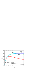
Figure 3: The function $W_{\|}^{\rm slab}$ for various thicknesses of the dielectric slab, with refractive index $n=2$. The uppermost curve is the result for a dielectric half-space, $W_{\|}^{\rm HS}$.

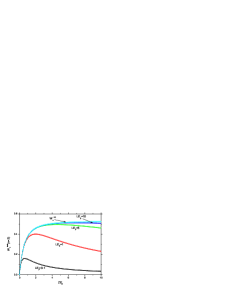
Figure 4: The function $W_{z}^{\rm slab}$ for various thicknesses of the slab, with refractive index $n=2$. The uppermost curve is for a dielectric half-space, i.e. for $LE_{ji}\rightarrow\infty$.

In Fig. 3 we show how the shift varies for different refractive indices if we fix the thickness of the slab at $LE_{ji}=1$. In practice values of $LE_{ji}\sim 10$ might be more realistic, but for those the energy shift is almost indistinguishable from the one for a dielectric half-space, as evident from Figs. 3 and 4.

Fig. 5 shows $W_{z}$ for various refractive indices $n=1.5,3,5,10$, and we have also included the limit of a perfect reflector, $n\rightarrow\infty$, labeled as $W_{z}^{\rm PR}$.

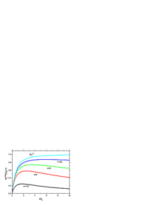
Figure 5: The function $W_{z}^{\rm slab}$ for a slab of thickness $LE_{ji}=1$ and various values of the refractive index, $n=1.5,3,5,10$. The uppermost curve $W_{z}^{\rm PR}$ is the result for a perfect reflector, i.e. for $n\rightarrow\infty$.

Furthermore, one can see how the energy shift varies with the thickness of the slab $LE_{ji}$. In Fig. 6, we have plotted $W_{z}$ as a function of slab thickness for various fixed surface-atom separations, fixing the refractive index at $n=2$.

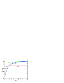
Figure 6: The function $W_{z}^{\rm slab}$ as a function of $LE_{ji}$, for an atom located at various fixed distances $\mathcal{Z}E_{ji}=1,5,10$ from the surface. The slab has a refractive index of $n=2$.

For Fig. 7 we have fixed the atom’s position at $\mathcal{Z}E_{ji}=8$ in the retarded regime, and shown how $W_{z}^{\rm slab}$ varies with the slab thickness for various values of the refractive index $n$. This shows again that the retarded Casimir-Polder force has a well-defined and analytic limit for $L\rightarrow 0$.

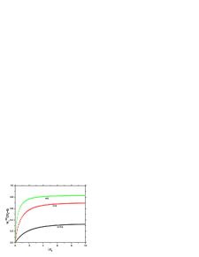
Figure 7: The function $W_{z}^{\rm slab}$ as a function of $LE_{ji}$, for an atom located at a distance $\mathcal{Z}E_{ji}=8$ from the slab and various values for the refractive index $n=1.5,3,5$. In the limit $n\rightarrow\infty$ this function approaches a unit step function.

Appendix A Mode functions

Throughout this paper we have adopted the same notation as in completeness , where $\mathbf{k}^{\pm}$ is the wave vector in vacuum

$$\mathbf{k}^{\pm}=(k_{x},k_{y},\pm k_{z})=(\mathbf{k}_{\parallel},\pm k_{z}),$$ (43)

and $\mathbf{k}_{\mathrm{d}}^{\pm}=(\mathbf{k}_{\parallel},\pm k_{\rm zd})$ is the wave vector inside the dielectric slab. The $z$-components of the wave vectors in free-space and dielectric are related through Snell’s law by

$$k_{\rm zd}=\sqrt{(n^{2}-1)k^{2}_{\|}+n^{2}k_{z}^{2}},$$ (44)

and in reverse

$$k_{z}=\frac{1}{n}\sqrt{k_{\rm zd}^{2}-(n^{2}-1)k^{2}_{\parallel}},$$ (45)

which are always positive.

The vector mode functions can be written as a product of a polarization vector and a scalar mode function,

$${\bf f}_{\mathbf{k}\lambda}(\mathbf{r})=\hat{\bf e}_{\lambda}\,f_{\mathbf{k}\lambda}(\mathbf{r})$$ (46)

We work with the transverse electric (TE) mode, for which the electric field is perpendicular to the plane of incidence,

$$\hat{\bf e}_{\rm TE}=(-\Delta_{\parallel})^{-1/2}(-i\partial_{y},i\partial_{x},0)\;,$$ (47)

and the transverse magnetic (TM) mode, for which the magnetic field is perpendicular to the plane of incidence,

$$\hat{\bf e}_{\rm TM}=(\Delta\Delta_{\parallel})^{-1/2}(-\partial_{x}\partial_{z},-\partial_{y}\partial_{z},\Delta_{\parallel})\;.$$ (48)

The momentum space representations $\hat{\bf e}_{\lambda}(\mathbf{k}^{\pm})$ of the polarization vectors are obtained by applying the above differential operators to a plane wave $e^{\rm i\mathbf{k}^{\pm}\cdot\mathbf{r}}$.

The scalar mode functions for travelling left-incident modes read

$$f_{\mathbf{k}\lambda}^{L}({\bf r})=N\left\{\begin{array}[]{ll}e^{i{\bf k}^{+}\cdot{\bf r}}+R_{\lambda}e^{i{\bf k}^{-}\cdot{\bf r}},&\quad z\leq-L/2\\ I_{\lambda}e^{i{\bf k}_{d}^{+}\cdot{\bf r}}+J_{\lambda}e^{i{\bf k}_{d}^{-}\cdot{\bf r}},&\quad|z|\leq L/2\\ T_{\lambda}e^{i{\bf k}^{+}\cdot{\bf r}},&\quad z\geq L/2\end{array}\right.$$ (49)

for any polarization $\lambda=TE,TM$. The normalization constant is $N=(2\pi)^{-3/2}$, and the remaining coefficients are obtained from the continuity conditions (3); in particular,

$$R_{\lambda} = r_{\lambda}\frac{1-e^{2{\rm i}k_{\rm zd}L}}{1-r_{\lambda}^{2}e^{2{\rm i}k_{\rm zd}L}}\ e^{-{\rm i}k_{z}L}$$ (50)

$$T_{\lambda} = \frac{1-r_{\lambda}^{2}}{1-r_{\lambda}^{2}e^{2{\rm i}k_{\rm zd}L}}\ e^{{\rm i}(k_{\rm zd}-k_{z})L}$$ (51)

where

$$r_{\rm TE}=\frac{k_{z}-k_{\rm zd}}{k_{z}+k_{\rm zd}}\quad{\rm and}\quad r_{\rm TM}=\frac{n^{2}k_{z}-k_{\rm zd}}{n^{2}k_{z}+k_{\rm zd}}\;.$$ (52)

The right-incident modes can be obtained straightforwardly from the left-incident modes, by simply inverting the $z$-axis and taking $z\rightarrow-z$.

$$f_{\mathbf{k}\lambda}^{R}(\mathbf{r})=N\left\{\begin{array}[]{ll}T_{\lambda}e^{i\mathbf{k}^{-}\cdot\mathbf{r}}&\quad z\leq-L/2\\ I_{\lambda}e^{i\mathbf{k}_{d}^{-}\cdot\mathbf{r}}+J_{\lambda}e^{i{\bf k}_{d}^{+}\cdot\mathbf{r}}&\quad|z|\leq L/2\\ e^{i\mathbf{k}^{-}\cdot\mathbf{r}}+R_{\lambda}e^{i\mathbf{k}^{+}\cdot{\bf r}}&\quad z\geq L/2\;.\end{array}\right.$$ (53)

The trapped modes are given by

$$f_{\mathbf{k}\lambda}^{S,A}({\bf r})=M_{\lambda}\left\{\begin{array}[]{ll}\pm L^{S,A}_{\lambda}e^{{\rm i}\mathbf{k}_{\|}\cdot\mathbf{r}+\kappa z},&\quad z\leq-L/2\\ e^{i\mathbf{k}_{d}^{+}\cdot\mathbf{r}}\pm e^{i\mathbf{k}_{d}^{-}\cdot\mathbf{r}},&\quad|z|\leq L/2\\ L^{S,A}_{\lambda}e^{{\rm i}\mathbf{k}_{\|}\cdot\mathbf{r}-\kappa z},&\quad z\geq L/2\end{array}\right.$$ (54)

where the $\pm$ signs apply to the symmetric (S) and antisymmetric (A) modes, respectively, and $\kappa=|{\rm i}k_{z}|\geq 0$. Note that for trapped modes the polarization vector (48) is complex and no longer of unit length. The normalization constants are

$$M_{\rm TE} = \frac{1}{4\pi\sqrt{n^{2}\frac{L}{2}+\frac{1}{\kappa}\left(\frac{k_{\parallel}}{k}\right)^{2}}}$$ (55)

$$M_{\rm TM} = \frac{1}{4\pi\sqrt{n^{2}\frac{L}{2}+\frac{1}{\kappa}\frac{n^{2}k_{\|}^{2}}{k_{\|}^{2}+n^{2}\kappa^{2}}}}\;,$$ (56)

and by imposing the continuity conditions (3) we obtain the coefficients $L^{S,A}_{\lambda}$

$$L^{S}_{TE} = 2\cos\left(\frac{k_{\rm zd}L}{2}\right)e^{\kappa L/2}$$ (57)

$$L^{A}_{TE} = 2{\rm i}\sin\left(\frac{k_{\rm zd}L}{2}\right)e^{\kappa L/2}$$ (58)

$$L^{S}_{TM} = 2n\cos\left(\frac{k_{\rm zd}L}{2}\right)e^{\kappa L/2}$$ (59)

$$L^{A}_{TM} = 2n{\rm i}\sin\left(\frac{k_{\rm zd}L}{2}\right)e^{\kappa L/2}\;.$$ (60)

The dispersion relations that arise from the simultaneous application of all matching conditions in Eq. (3) to the symmetric (S) and antisymmetric (A) modes, with two polarizations $\lambda$ each, read

$$\kappa=\left\{\begin{array}[]{ll}k_{\rm zd}\tan(k_{\rm zd}L/2)&\quad\mbox{for (S), }\lambda=\mbox{TE,}\\ -k_{\rm zd}\cot(k_{\rm zd}L/2)&\quad\textrm{for (A), }\lambda=\mbox{TE,}\\ -k_{\rm zd}\cot(k_{\rm zd}L/2)/n^{2}&\quad\textrm{for (S), }\lambda=\mbox{TM,}\\ k_{\rm zd}\tan(k_{\rm zd}L/2)/n^{2}&\quad\textrm{for (A), }\lambda=\mbox{TM,}\end{array}\right.$$ (61)

where

$$\kappa=\frac{1}{n}\sqrt{(n^{2}-1)k^{2}_{\parallel}-k_{\rm zd}^{2}}\;.$$ (62)

Appendix B Electrostatic calculation of the electrostatic shift

In order to have an independent check of our general formula for the energy-shift, which in the non-retarded limit takes the form (35), we shall derive the same non-retarded shift purely by means of a classical electrostatics. If retardation can be ignored, the energy shift of the atom is simply the electrostatic energy of the atomic dipole when placed near the dielectric slab.

If the electrostatic potential $\Phi(r)$ generated by a unit point charge at a position $\mathbf{r}^{\prime}$ is known, then the electrostatic energy of an atomic dipole located at $\mathbf{r}_{0}$ is (cf. e.g. cyl for a more detailed discussion):

$$\Delta E_{{\rm es}}=\left.\frac{1}{2}\sum_{i=\{x,y,z\}}\langle\mu_{i}^{2}\rangle\mathbf{\nabla}_{i}\mathbf{\nabla}^{\prime}_{i}\;\Phi_{H}(\mathbf{r},\mathbf{r}^{\prime})\right|_{\mbox{\footnotesize${\bf r}={\bf r}_{0},{\bf r}^{\prime}={\bf r}_{0}$ }}\;.\\$$ (63)

Here the harmonic function $\Phi_{H}(\mathbf{r},\mathbf{r}^{\prime})$ is the difference between the potential $\Phi(r)$ generated by the point charge at $\mathbf{r}^{\prime}$ and the potential that would be generated by that charge in unbounded space, so as to exclude from $\Delta E_{{\rm es}}$ the (infinite) electrostatic self-energies that do not depend on the relative position of the dipole and the slab. As $\Phi_{H}(\mathbf{r},\mathbf{r}^{\prime})$ is a solution of the Laplace equation and must vanish for $z\rightarrow\pm\infty$, it must be of the form:

$$\Phi_{H}(\mathbf{r},\mathbf{r}^{\prime})=\int_{-\infty}^{\infty}\mathrm{d}k_{x}\int_{-\infty}^{\infty}\mathrm{d}k_{y}\;e^{{\rm i}k_{x}x+{\rm i}k_{y}y}$$

$$\times\left\{\begin{array}[]{ll}C_{1}(\mathbf{k}_{\parallel},\mathbf{r}^{\prime})\;e^{k_{\parallel}z}&\mbox{for\ }z\leq-L/2\\ C_{2}(\mathbf{k}_{\parallel},\mathbf{r}^{\prime})\;e^{k_{\parallel}z}+C_{3}(\mathbf{k}_{\parallel},\mathbf{r}^{\prime})\;e^{-k_{\parallel}z}&\mbox{for\ }|z|\leq L/2\\ C_{4}(\mathbf{k}_{\parallel},\mathbf{r}^{\prime})\;e^{-k_{\parallel}z}&\mbox{for\ }z\geq L/2\;.\end{array}\right.$$ (67)

The coefficients $C_{1-4}(\mathbf{k}_{\parallel},\mathbf{r}^{\prime})$ are easily worked out by applying the continuity conditions (3) to this electrostatic problem. Straightforward manipulations then give

$$\Phi_{H}=-\frac{1}{4\pi\varepsilon_{0}}\frac{\varepsilon-1}{\varepsilon+1}\int_{0}^{\infty}\mathrm{d}k\;J_{0}(k\rho)\;e^{-k(z+z^{\prime}-L)}$$

$$\times\frac{1-e^{-2kL}}{1-(\frac{\varepsilon-1}{\varepsilon+1})^{2}e^{-2kL}}\mbox{\ \ \ for\ }z,z^{\prime}>L/2\;,$$ (68)

with $\rho=\sqrt{(x-x^{\prime})^{2}+(y-y^{\prime})^{2}}$. It is instructive to rewrite the denominator as a geometric series

$$\frac{1}{1-\left(\frac{\varepsilon-1}{\varepsilon+1}\right)^{2}e^{-2kL}}=\sum_{n=0}^{\infty}\left[\left(\frac{\varepsilon-1}{\varepsilon+1}\right)^{2}e^{-2kL}\right]^{n}$$

and note that (GR, , Eq. 6.611(1.))

$$\int_{0}^{\infty}\mathrm{d}k\;J_{0}(k\rho)\;e^{-k(z-z^{\prime})}=\frac{1}{\sqrt{\rho^{2}+(z-z^{\prime})^{2}}}\;,$$

which reveals that $\Phi_{H}(\mathbf{r},\mathbf{r}^{\prime})$ can be understood as being due to a series of image charges generated by repeated reflections between the two interfaces of the slab Smythe . However, expression (68) is more useful for calculations; substituting it into Eq. (63) gives for the electrostatic energy shift

$$\Delta E_{{\rm es}}=-\frac{1}{16\pi\varepsilon_{0}}\;\frac{\varepsilon-1}{\varepsilon+1}\sum_{j}\left(2|\mu_{\perp}|^{2}+|\mu_{\|}|^{2}\right)$$

$$\times\int_{0}^{\infty}\mathrm{d}k\;k^{2}\;e^{-2\mathcal{Z}k}\frac{1-e^{-2kL}}{1-\left(\frac{\varepsilon-1}{\varepsilon+1}\right)^{2}e^{-2kL}},$$ (69)

which, upon replacing $\varepsilon=n^{2}$, is in agreement with Eq. (35).

- (1) H. Chan, V. Aksyuk, R. Kleiman, D. Bishop and F. Capasso, Phys. Rev. Lett., 87, 211801, (2001).
- (2) H. Casimir and D. Polder, Phys. Rev., 73, 360–372, (1948).
- (3) J. Obrecht, R. Wild, M. Antezza, L. Pitaevskii, S. Stringari and E. Cornell, Phys. Rev. Lett. 98, 063201, (2007)
- (4) H. Khosravi and R. Loudon, Proc. R. Soc. London, Ser. A 436, 373 (1992).
- (5) A. Abrikosov, L. Gorkov and I. Dzyaloshinski, Methods of Quantum Field Theory in Statistical Physics, Dover (1975)
- (6) S. Buhmann and D. Welsch, Progress in quantum electronics, 31, 51-130, (2007).
- (7) A. Contreras Reyes and C. Eberlein, Phys. Rev. A 79, 043834 (2009).
- (8) W. Żakowicz and A. Błȩdowski, Phys. Rev. A 52, 1640 (1995).
- (9) C. Eberlein and D. Robaschik, Phys. Rev. Lett. 92, 233602 (2004).
- (10) C. Eberlein and S. Wu, Phys. Rev. A 68, 033813 (2003).
- (11) We work in natural units, setting and unless explicitly indicated.
- (12) S. Wu and C. Eberlein, Proc. R. Soc. Lond, Ser. A 455, 2487 (1999).
- (13) Handbook of Mathematical Functions, edited by M. Abramowitz and I. Stegun (US GPO, Washington, DC, 1964).
- (14) M. Bordag, Phys. Rev. D 76, 065011 (2007)
- (15) The non-retarded energy shift of an atom in front of a perfectly reflecting mirror is given by and in Eq. (41).
- (16) C. Eberlein and R. Zietal, Phys. Rev. A 75, 032516 (2007).
- (17) This is also discussed in Section 5.303 of W.R. Smythe, Static and Dynamic Electricity (Taylor & Francis, London, 1989), 3rd ed., where the potential is worked out for and on opposite sides of the slab, i.e. for and .
- (18) I.S. Gradshteyn and I.M. Ryzhik, Table of Integrals, Series, and Products, edited by A. Jeffrey (Academic Press, London, 1994), 5th ed.