Convergent flow in a two–layer system and mountain building

Abstract

With the purpose of modelling the process of mountain building, we investigate the evolution of the ridge produced by the convergent motion of a system consisting of two layers of liquids that differ in density and viscosity to simulate the crust and the upper mantle that form a lithospheric plate. We assume that the motion is driven by basal traction. Assuming isostasy, we derive a nonlinear differential equation for the evolution of the thickness of the crust. We solve this equation numerically to obtain the profile of the range. We find an approximate self–similar solution that describes reasonably well the process and predicts simple scaling laws for the height and width of the range as well as the shape of the transversal profile. We compare the theoretical results with the profiles of real mountain belts and find an excellent agreement.

I Introduction

Mountain ranges are one of the most striking features of the Earth and their origin and evolution have been investigated for a long time. It is known that the lithosphere (the outer solid layer of the Earth) is a two layer structure in which the crust rests on the denser upper mantle, being separated by the Mohorovi$\rm\check{c}$i$\rm\acute{c}$ discontinuity (called Moho). The lithosphere is divided into several approximately rigid plates that rest on the hotter and more fluid asthenosphere. The relative motion of these plates is the cause of mountain building, because of the shortening and consequent thickening of the crust that occurs when two continental plates collide (see Fig. 1 for a sketch) or when an oceanic plate is subducted beneath a continent. On the timescale of the orogenic processes the lithosphere is in local hydrostatic equilibrium (a condition called isostasy) that implies that the visible regional topography is accompanied by a corresponding anti-topography (called root) of the Moho.

Clearly mountain builiding is an important problem that involves many disciplines and interests a broad range of scientists. To attempt a realistic and detailed theoretical description of mountain building is an exceedingly complex task (see for example the recent review by Avouac avouac07 where the field data are discussed) because across the lithosphere there are large variations of the temperature, density and rheological parameters as well as other properties (many of which, to compound the issue, are poorly known). To this should be added the complications due to the geometry and the time dependence of the motion of the plates. Since the pioneering work of England and McKenzie england82 ; england83 several models called collectively ‘thin sheet models’ that treat the lithosphere as a thin viscous layer or layers have been developed to take into account in a simplified way some of the above mentioned features (a classification can be found in Refs. medvedev99a, ; medvedev99b, ). These models have been used to describe mountain building, mainly by means of extensive and detailed numerical simulations that deal with specific ranges.

The basic phenomena that govern the large scale evolution of mountain belts are the spreading flow at the depth of the roots together with isostasy and crustal shortening. The profile of the ridge is determined by the dynamic balance between buoyancy and viscous forces. Based on these ideas Gratton gratton89 used dimensional arguments to derive scaling laws for the evolution of the height and the width of a mountain belt and argued that the evolution of the profile of a range is self–similar, even if he could not compute the exact shape. To this purpose he estimated the viscous forces assuming that the vertical gradient of the horizontal velocity takes place near the root. However, we shall show later that this assumption is not correct, since the whole lithospheric mantle is involved in the flow. As a consequence the scaling laws of Ref. gratton89, can not describe the evolution of mountain ranges.

More recently we investigated a related problem, namely the formation of a ridge by the convergent flow of a single liquid layer over a solid moving substrate perazzo08 ; perazzo09 ; gratton09 , and found that for small time $T$ there is a self–similar regime in which the height and the width of the range scale as $T^{1/2}$ regardless of the asymmetry of the flow and the rheology of the liquid. For large time, however, a different self–similar regime is achieved in which the height and the width follow the scaling laws obtained in Ref. gratton89, . Other researchers have also investigated independently this problem theoretically and with a laboratory model buck94 as well as numerically willett99 ; medvedev02 .

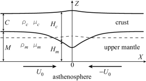
Figure 1: Geometry of the two layer model employed to describe the formation of a ridge. The line separating the crust and the upper mantle is the Moho. The dashed line represents an isobar.

Following our previous works we here reduce the problem to its basic essentials, taking into account the two–layer structure of the lithosphere but disregarding rheological and geometrical details. For simplicity we assume a Newtonian rheology for the crust and for the lithospheric mantle, and that the problem depends on a single horizontal cartesian coordinate. We also ignore erosion. In this way we find approximate analytic solutions, scaling laws and the asymptotic behavior of the process, thus achieving a deeper physical understanding of the process.

This paper is organized as follows. In section II we describe the assumptions and we derive the governing equations. In section III we derive the self–similar regime developed in the process. In section IV we compare the self–similar theoretical profile with the topography of several mountain ranges. Finally in section V we discuss our work, whose main conclusions are: (1) the simple two–layer model describes quite well the evolution of many mountain belts, (2) their profiles have a universal shape, and (3) to a good approximation the evolution is self–similar, with the height and width increasing as $T^{1/2}$.

II The two–layer model

Our aim is to describe the essentials of the mountain building process, using a model as simple as possible, in order to clarify the basic physics involved. To this purpose we consider a two layer liquid film as shown in Fig. 1 and we assume for simplicity plane symmetry. The upper layer (the crust) has viscosity $\mu_{c}$, density $\rho_{c}$ and thickness $H_{c}(X,T)$. The lower one (the upper mantle) has viscosity $\mu_{m}$, density $\rho_{m}$ and thickness $H_{m}(X,T)$. Typically for a continental plate $\rho_{c}\approx 2.7$ g/cm³, $\rho_{m}\approx 3.2$ g/cm³, and $\mu_{c}\gg\mu_{m}$.

Initially, both layers are uniform and $H_{c}(X,0)=C$ and $H_{m}(X,0)=M$. To model the basal traction that is believed to drive the plate motion we assume that at $T=0$ the bottom of the lithosphere ($Z=0$) starts moving with a prescribed velocity $U_{b}(X)$. We next assume isostasy, which means that for $0\leq Z\leq H_{m}$ (see the dashed line in Fig. 1) the pressure does not depend on $X$. Notice that this implies that as the thickness of the crust increases, part of the mass of the lithospheric mantle crosses the boundary between the lithosphere and the asthenosphere. As a consequence the mass of the lithospheric mantle is not conserved.

To derive the governing equations we assume a slow viscosity–dominated flow and employ a slight generalization of the well–known lubrication approximation (see for example Refs. buckmaster77, ; huppert82, ; oron97, ) to take into account the motion of the bottom of the lithosphere. We neglect inertia and assume that the slope of the free surface is gentle, so that the horizontal components of the velocities of the fluids are much larger than the vertical ones and that their vertical gradients are much larger than the horizontal gradients. In this way the Stokes equation takes the form

$$\frac{\partial P}{\partial X}=\mu_{m}\frac{\partial^{2}U}{\partial Z^{2}},\quad\frac{\partial P}{\partial Z}=\rho_{m}g,$$ (1)

for $0\leq Z\leq H_{m}$, and

$$\frac{\partial P}{\partial X}=\mu_{c}\frac{\partial^{2}U}{\partial Z^{2}},\quad\frac{\partial P}{\partial Z}=\rho_{c}g,$$ (2)

for $H_{m}\leq Z\leq H_{m}+H_{c}$. In these equations $P$ is the pressure, $U(X,Z,T)$ is the horizontal velocity and $g$ is the gravity. The second equations in (1) and (2) mean that the pressure is hydrostatic; integrating them and using the isostasy condition ($\partial P/\partial X=0$ for $0\leq Z\leq H_{m}$) we find $\rho_{m}\partial H_{m}/\partial X=-\rho_{c}\partial H_{c}/\partial X$. Integrating this equation and using the initial condition we obtain

$$H_{m}=M+\frac{\rho_{c}}{\rho_{m}}(C-H_{c}).$$ (3)

This allows elimination of $H_{m}$ thus yielding an equation for the single dependent variable $H_{c}$.

To derive the velocity profile we assume that $U(Z=0)=U_{b}$, that the velocity and the shear stress are continuous at $Z=H_{m}$, and that the shear stress vanishes at $Z=H_{m}+H_{c}$. Then we integrate twice the first equations in (1) and (2) with respect to $Z$ to obtain

$$U=\left\{\begin{array}[]{ll}U_{b}-\frac{g\rho_{c}}{\mu_{m}}H_{c}\left(\frac{\partial H_{c}}{\partial x}+\frac{\partial H_{m}}{\partial x}\right)Z,&0\leq Z\leq H_{m}\\ &\\ U_{b}+\frac{g\rho_{c}}{\mu_{c}}\left(\frac{\partial H_{c}}{\partial x}+\frac{\partial H_{m}}{\partial x}\right)\left[\frac{1}{2}\left(Z-H_{m}\right)\left(Z-2H_{c}-H_{m}\right)-\frac{\mu_{c}}{\mu_{m}}H_{c}H_{m}\right],&H_{m}\leq Z\leq H_{m}+H_{c}\end{array}\right.$$ (4)

Notice that the velocity profile is linear in the lithospheric mantle and parabolic in the crust and that the average shear stress in the crust is exactly half of that in the lithospheric mantle. This means that in most situations the velocity drop in the crust is a small fraction of that within the mantle. As we will show later these features of the velocity field are crucial to determine the scaling laws for the growth of the range.

We define the vertically averaged velocity in the crust as

$$V_{c}=\frac{1}{H_{c}}\int_{H_{m}}^{H_{m}+H_{c}}U\,dZ.$$ (5)

We set $U_{b}(X)=U_{0}u(X)$, where $U_{0}$ is the maximum basal velocity so that $u$ verifies $|u|\leq 1$. Next we introduce the following dimensionless quantities

$$h=H_{c}/C,\quad v=V_{c}/U_{0},\quad x=X/X_{0},\quad t=TU_{0}/X_{0}.$$ (6)

Here the horizontal scale $X_{0}$ is given by

$$X_{0}=(1-\frac{\rho_{c}}{\rho_{m}})\frac{\rho_{c}gMC^{2}}{\mu_{m}U_{0}}.$$ (7)

Finally inserting the second of (4) in (5) and using (6), we obtain

$$v=u-\left(1+\frac{\rho_{c}C}{\rho_{m}M}\right)h\frac{\partial h}{\partial x}-\frac{C}{M}\left(\frac{\mu_{m}}{3\mu_{c}}-\frac{\rho_{c}}{\rho_{m}}\right)h^{2}\frac{\partial h}{\partial x}.$$ (8)

This equation together with the continuity equation

$$\frac{\partial h}{\partial t}+\frac{\partial(vh)}{\partial x}=0,$$ (9)

govern the dimensionless thickness of the crust. The preceding equations can be easily extended to two dimensions to deal with more general geometries.

To describe the convergence of two plates we make the simplest assumption: $u(x)=1$ for $x<0$ and $u(x)=-1$ for $x>0$. In this way the thickness of the crust starts to increase in the region of convergence. The initial condition is $h(x,0)=1$, and the boundary conditions are $h(\pm\infty,t)=1$. At $x=0$ we impose the continuity of $h$ and $v$.

In general this problem must be solved numerically. In Fig. 2 we show some solutions. All the results shown in figures 2, 3 and 4 were calculated for $C=30$ km, $M=100$ km, $\rho_{c}=2700$ kg/m³, $\rho_{m}=3200$ kg/m³ and $\mu_{c}/\mu_{m}=10$. These values are representative of those found in the lithosphere, so that the results shown can be applied in general to the mountain building process.

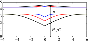
Figure 2: (Color online) Numerical solutions of (8–9) with $u(x)=\pm 1$ for $x\lessgtr 0$ and $h(x,0)=1$, for $t=$0.25, 1.31 and 4.00 ($C=30$ km, $M=100$ km, $\rho_{c}=2700$ kg/m³, $\rho_{m}=3200$ kg/m³, $\mu_{c}/\mu_{m}=10$).

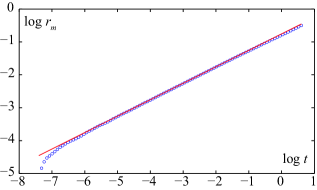
Figure 3: (Color online) Evolution of the maximum relief $r_{m}=r(0,t)$. The circles correspond to the numerical solution with the same parameters as in Fig. 2; the straight line is $r_{ss}(0,t)$.

III Self–similar regime

We now seek the asymptotics of the problem for small $t$. We define $r=(1-\rho_{c}/\rho_{m})(h-1)$, then $R\equiv Cr$ is the visible topography of the range. Since at the beginning of the phenomenon $h-1\ll 1$, the Eqs. (8) and (9) can be linearized, and with the assumption $u(x)=\pm 1$ for $x\lessgtr 0$ reduce to

$$\frac{\partial r}{\partial t}=\pm\frac{\partial r}{\partial x}+\left(1+\alpha\right)\frac{\partial^{2}r}{\partial x^{2}},\quad x\gtrless 0,$$ (10)

where $\alpha=\mu_{m}C/3\mu_{c}M$. With typical values for the lithosphere $\alpha\approx 10^{-2}$, so that it can be neglected and in this approximation the problem depends only on the scales $X_{0}$, $C$ and $U_{0}$.

A solution of Eq. (10) as an infinite series similar to that given in Ref. perazzo08, exists (see the Appendix A). Here we shall show an approximate self–similar solution $r_{ss}$ that for $r\ll 1$ represents the asymptotics of the full solution. It is given by

$$r_{ss}\equiv\left(1-\frac{\rho_{c}}{\rho_{m}}\right)\frac{2\sqrt{t}}{\sqrt{1+\alpha}}f(\psi),$$ (11)

where

$$f(\psi)=\frac{e^{-\psi^{2}}}{\sqrt{\pi}}-\psi\,\text{erfc}(\psi),\quad\psi\equiv\frac{x}{2\sqrt{(1+\alpha)t}}.$$ (12)

Here erfc is the complementary error function. According to this solution the height and the width of the ridge follow a simple $t^{1/2}$ scaling. We define (arbitrarily) the dimensionless width of the ridge as $w=2x(\psi=1)=4\sqrt{(1+\alpha)t}$ (so the width is the distance between the two points in which the height is 9% of the peak height). Then the height and the width $W=X_{0}w$ of the ridge are given by

$$R=\frac{2U_{0}}{\sqrt{\pi(1+\alpha)}}\sqrt{\left(1-\frac{\rho_{c}}{\rho_{m}}\right)\frac{\mu_{m}}{\rho_{c}gM}}T^{1/2},$$ (13)

$$W=\frac{4C}{\sqrt{1+\alpha}}\sqrt{\left(1-\frac{\rho_{c}}{\rho_{m}}\right)\frac{\rho_{c}gM}{\mu_{m}}}T^{1/2}.$$ (14)

It is interesting that $W$ depends on $C$, but not on $U_{0}$. On the other hand $R$ depends on $U_{0}$ and is nearly independent on $C$ (it depends on $C$ only through $\alpha$). Notice also that the aspect ratio $\theta=W/R$ of the ridge is constant and equal to

$$\theta=\frac{2\sqrt{\pi}\rho_{c}gCM}{\mu_{m}U_{0}}.$$ (15)

Within the uncertainties in the parameters involved, these formulae give the correct order of magnitude of $R$ and $W$ for real mountain ranges.

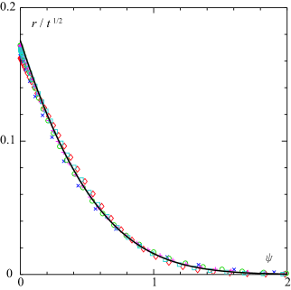
Figure 4: (Color online) Scaled relief of the numerical solutions (circles) for $t=1.4\times 10^{-6}$ ($\times$), $5.7\times 10^{-5}$ ($\circ$), $2.3\times 10^{-3}$ ($+$), $9.7\times 10^{-2}$ ($\square$) and $6.2\times 10^{-1}$ ($\lozenge$). The solid line is $r_{ss}/\sqrt{t}$.

It is interesting to compare this approximate self–similar solution with the numerical solutions of the full nonlinear problem (8–9). In Fig. 3 we show the numerical $r(0,t)$ and $r_{ss}(0,t)$. In Fig. 4 we compare the numerical solutions with the solution (11). From these figures it can be appreciated that the self–similar solution (11–12) describes quite well the shape and the evolution of the ridge, even for quite large $t$ when it might be expected to fail (notice that the last circle of Fig. 3 corresponds to $h(0,t=4)=3$, and that $h(0,t=0.62)=1.82$ for the last profile in Fig. 4). In terms of the topography this implies that mountain ranges whose height does not exceed approximately 5 km are well described by (11–12). We then conclude that the self–similar solution describes reasonably well the solution of the full nonlinear problem up to this point. We observe that for the parameters of the numerical calculations shown in these figures $h(0,t)=4.95$ corresponds to the root of the ridge touching the asthenosphere, after which the relief can not increase anymore.

IV Comparison with real mountain ranges

It is interesting to compare the present theory with the real profiles of mountain ranges. However at this point it is convenient to point out that some mountain systems are not linear so that they can not be described by the present theory. For our comparisons we have used the digital elevation data GTOPO30 (these data are available in the website of the U.S. Geological Survey’s Earth Resources Observation and Science (EROS) Center) to obtain locally averaged profiles of 10 approximately rectilinear segments of the Alps, Andes (2 segments), Barisan Mountains in Sumatra, Caucasus (2 segments), New Zealand Alps, Pyrenees and Urals (2 segments). For each segment we have drawn 50 transversal profiles of 101 points each. All the 10 segments we examined have the same “pagoda roof” profile. However 4 of them (one segment of the Andes, Caucasus and Urals, and the New Zealand Alps) are markedly asymmetric, having one side steeper than the other; in addition the foot of the steeper side is lower than the other.

In Fig. 5 we show the average of the 50 profiles of a segment of the Pyrenees along with the best fit of these data to $af((X-b)/c)+d$, where $f$ is given in (12) and $a$, $b$, $c$ and $d$ are constant lengths.

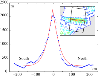
Figure 5: (Color online) Comparison of the average topography (dots) of a segment of the Pyrenees (shown in the inset) with the theoretical profile (11–12). The full line is $af((X-b)/c)+d$ where $a$, $b$, $c$ and $d$ are constants lengths determined by fitting the actual topography.

In Fig. 6 we show the theoretical profile (11–12) and the 6 more symmetric average profiles. To merge these profiles in a single graph we plotted $(R_{i}-d_{i})/a_{i}$ vs. $(X_{i}-b_{i})/c_{i}$ ($i=1,\ldots,6$). To obtain the constants $a_{i}$, $b_{i}$, $c_{i}$, $d_{i}$ we followed the same procedure as we did for the Pyrenees. It can be appreciated that the self–similar approximate solution gives an excellent fit to the actual shapes.

V Discussion and conclusions

As can be seen in figures 5 and 6 the agreement of the profiles of actual ranges with the self–similar shape is very good, even for a very ancient range as the Urals. However some explanations are opportune.

The theoretical profiles are sharply peaked due to the discontinuity of $u(x)$ at $x=0$. It is easy to solve numerically the problem with a continuous transition of $u(x)$. We have done it assuming that $u=\tanh(x/w_{0})$ where $2w_{0}$ is the width of the transition. In figure 8 we compare the numerical solution for $w_{0}=0.4$ (this value was chosen for better visibility) with the solution for the discontinuous $u$ case for the same time ($t=1.31$). We see that a continuous transition leads to the same profile, except near the top where it is rounded. The width of this rounded region is always $\approx 2w_{0}$, but since the width of the range increases as $t^{1/2}$ the difference between the continuous and discontinuous cases reduces with time. We conclude that the self–similar solution (11–12) describes increasingly well the profile.

The actual topographies shown in figures 5 and 6 are the result of averaging all the transversal profiles of each range. All the profiles employed to prepare these figures have a peak, but on averaging them a rounded summit is obtained. Notice that the noise present in the data due to the local topographical accidents (that occur near the surface of the crust and are not a consequence of the average lithospheric flow we are considering) introduces a horizontal scale $w_{\mathrm{noise}}$ of a few kilometers, that sets a limit to the size of the features that can be compared with the theoretical model. Then the rounded top of these figures whose sizes are of the order of $w_{\mathrm{noise}}$ do not contradict the sharp theoretical profile. In addition, this fact suggests that the transition of the basal velocity occurs on a horizontal scale shorter than $2w_{\mathrm{noise}}$.

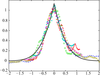
Figure 6: (Color online) Comparison of the theoretical profile from the model with the Andes ($+$), Caucasus ($\circ$), Alps ($\ast$), Urals ($\times$), Pyrenees ($\square$) and Barisan Mountains ($\lozenge$).

In our calculations we have assumed for simplicity a perfect symmetry. However it is not difficult to extend our model to a non–symmetric situation in which $|u|$ as well as $C$ are different in each side of the ridge. To appreciate the effects of both kinds of asymmetries we show in figure 7 the numerical solutions for the symmetric case and those corresponding to a nonsymmetric basal velocity ($u=1.9$ for $x<0$ and $u=-0.1$ for $x>0$) and to a nonsymmetric thickness of the crust ($h(x<0,0)=0.9$ and $h(x>0,0)=1.1$), for $t=1.31$. The parameters have been chosen to ensure that in the three cases the added dimensionless mass is equal to $2t$. We can observe that regardless of the asymmetry the crest remains at $x=0$. For brevity we omit more details, that will be published elsewhere. We believe that the non–symmetric segments of the Andes, Caucasus, Urals and the New Zealand Alps can be reproduced by adequate choices of the parameters.

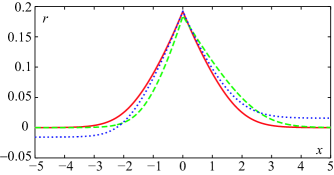
Figure 7: (Color online) Comparison of the solution for symmetric case (full line) with those for nonsymmetric basal velocity (dashed line) and nonsymmetric thickness of the crust (dotted line).

The present theory assumes a Newtonian rheology for the lithosphere, although it is believed that its behavior is non–Newtonian. In a recent article gratton09 we considered the effect of a power–law rheology in the one layer model of Ref. perazzo08, . We found that in the linear regime the maximum height and the width of the ridge increase as $t^{1/2}$ regardless of the rheological parameters. On the other hand the profile of the ridge depends on the rheology, but only weakly (see figure 4 of Ref. gratton09, ). The two layer model used here can be extended to include non–Newtonian behavior but to do this exceeds the scope of the present paper. However based on the results of one layer model we expect that similar results will be obtained for the two layer model since in the linear regime both models give analogous equations.

We do not take into account in our model the effect of erosion. Several authors have considered the role of glacial and fluvial erosion in the orogenic process, modeling the resulting redistribution of mass at large scale as a diffusive process (see for example Refs. burov07, ; burov09, and references therein). The inclusion in our model of this effect would modify the coefficient of the diffusion term $\partial^{2}r/\partial x^{2}$ in equation (10). This means that a self–similar solution of the same kind as (11) and (12) would result, but with different scales. Incidentally, this could be the explanation why our self–similar profile describes quite well all the ranges analyzed regardless of their erosion history. Notice also that this change should not modify the sharp apex of the ridge, so that a rounded summit will not result. We leave for future work a detailed investigation of the effects of erosion.

The present model can be easily generalized to include 3–D effects replacing $u$ by a two–dimensional vector $\mathbf{u}=\mathbf{u}(x,y)$ and $\partial/\partial x$ by the two–dimensional gradient operator $\nabla=(\partial/\partial x,\partial/\partial y)$. The 3–D character arises from the dependence of $\mathbf{u}$ on both cartesian coordinates. The resulting problem must then be solved numerically. The 3–D effects will be important in those parts of a range where the average curvature radius of the crest of the ridge is smaller than or of the order of its width. On the contrary, our results can be applied whenever the curvature radius is much larger than the width.

Figure 8: (Color online) Comparison of a profile for a continuous basal velocity ($w_{0}=0.4$, dotted line) with the discontinuous case (full line), for $t=1.31$.

The $t^{1/2}$ scaling law can be justified with a dimensional argument based on isostasy, conservation of the crustal mass during the shortening and the balance between gravitational and viscous stresses, entirely analogous to that employed in Ref. gratton89, . In that paper different scaling laws were obtained because the viscous stress was incorrectly estimated, since it was not realized the key feature of the two layer model dynamics, namely that the entire lithospheric mantle is involved.

Most of the papers about mountain building deal with specific ranges, chiefly the Himalaya–Tibet orogeny, that can not be described by the present model. It is interesting to compare the results of our two–layer model with those of one layer–models (see for example Medvedev medvedev02 and Perazzo and Gratton perazzo08 ), and those from the two–layer model of Royden royden96 . The one layer models considers a single viscous layer on a solid horizontal substrate with convergent motion. According to Ref. medvedev02, ; perazzo08, the height and the width of the wedge increase as $t^{\beta}$ and $t^{1-\beta}$ respectively. In Ref. medvedev02, it is found that $\beta$ decreases with time and that the evolution of the wedge can be divided into three phases. Initially, $\beta=1$ so that the wedge grows only in height. The second phase exhibits an almost self–similar growth in which $\beta=1/2$ so that the height and the width increase as $t^{1/2}$. For later times a last phase is achieved in which $\beta$ decreases below 0.4. In Ref. perazzo08, two self–similar regimes were found corresponding to $\beta=1/2$ for short times and to $\beta=1/4$ for large time. In our two–layer model and for realistic values of the thickness of the lithosphere we observe only a $t^{1/2}$ self–similar regime because the root touches the asthenosphere before significant departures from this regime occur. On the other hand a $\beta=1$ initial phase can be obtained in our two–layer model if we assume that the the basal velocity has a continuous transition whose horizontal extent is $2w_{0}$; this phase ends around $t=\frac{4}{\pi}w_{0}^{2}$ (for brevity we omit details). Thus the one–layer and our two–layer models yield power–laws for the evolution of the height and the width which have the same exponents, notice however that the factors are quite different.

The two–layer model of Royden royden96 considers only the crust, that is divided into an upper layer with uniform viscosity and a lower layer in which the viscosity decreases exponentially with the depth. The basal traction condition is assumed to hold at the bottom of the crust. It is shown that two regimes can occur. In the first, the crustal flow is directly coupled to the underlying mantle. In the second the upper crustal to mid crustal flow is decoupled from the underlying mantle. Which one of these regimes occur depends on the viscosity just above the Moho, which in turns depends on its depth. If no significant low–viscosity zone develops, crustal deformation is coupled to the motion of the underlying mantle, and a triangular mountain range develops. If a low–viscosity zone is initially absent but develops during crustal thickening a steep–sided flat–topped plateau ultimately forms. If a low viscosity zone is present in the lower crust prior to convergence, a wide orogen with low topographic relief develops. In the last two cases crustal flow is decoupled from the mantle except at the edges of the flat region. The triangular profiles that are obtained in the coupled mode look quite similar to those obtained here. Notice however that the simplicity of our model has allowed to obtain analytic formulae for the shape of the range and its scaling laws, not previously known. Furthermore, according to our two–layer model the flow within the crust should decouple from basal traction when the root touches the asthenosphere, being driven only by gravity, possibly yielding a flat–topped profile similar to those discussed in Ref. royden96, . We have not yet investigated this regime.

We conclude that the simple two layer model describes quite well the evolution of many mountain belts. Although the lithosphere is described by many parameters, to a good approximation the orogenic process involves only $U_{0}$, $C$ and the combination $X_{0}$ (Eq. (7)). Furthermore as long as $\mu_{m}\ll\mu_{c}$ the viscosity of the crust is not relevant, since most of the vertical gradient of the velocity occurs in the lithospheric mantle. The evolution of mountain belts is to good approximation self–similar and in the symmetric case the profile is given by (11–12).

*

Appendix A Linearized series solution

Introducing the scaled variables

$$\tilde{t}=t/(1+\alpha),\quad\tilde{x}=x/(1+\alpha),\quad\tilde{r}=r/(1+\alpha)$$

in equation (10) and following the procedure described in the Appendix of Ref. perazzo08, , we obtain the solution for $x>0$ as

$$\tilde{r}=\frac{e^{-s^{2}}}{\sqrt{\pi}}\left[2\sqrt{\tilde{t}}\,H_{-2}(s)+\sum_{j=1}^{\infty}\left(2\sqrt{\tilde{t}}\,\right)^{j}H_{-1-j}(s)\right],$$ (16)

where $s=(\tilde{t}+\tilde{x})/2\sqrt{\tilde{t}}$ and $H_{q}(s)$ denotes the Hermite function of order $q$. To obtain the solution for $x<0$ one must change $x$ for $-x$ in (16).

References

- (1) J. P. Avouac, “Dynamic processes in extensional and compressional settings – mountain building: from earthquakes to geological deformation,” in Crust and lithosphere dynamics, Treatise on Geophysics Vol. 6, edited by G. Schubert (Elsevier, Cambridge, 2007) pp. 377–439.
- (2) P. England and D. McKenzie, “A thin viscous sheet model for continental deformation,” Geophys. J. Internat. 70, 295–321 (1982).
- (3) P. England and D. McKenzie, “Correction to: a thin viscous sheet model for continental deformation,” Geophys. J. Internat. 73, 523–532 (1983).
- (4) S. E. Medvedev and Y. Y. Podladchikov, “New extended thin-sheet approximation for geodynamic applications-I. Model formulation,” Geophys. J. Internat. 136, 567–585 (1999).
- (5) S. E. Medvedev and Y. Y. Podladchikov, “New extended thin-sheet approximation for geodynamic applications-II. Two-dimensional examples,” Geophys. J. Internat. 136, 586–608 (1999).
- (6) J. Gratton, “Crustal shortening, root spreading, isostasy, and the growth of orgenic belts: A dimensional analysis,” J. Geophys. Res. 94, 15627–15634 (1989).
- (7) C. A. Perazzo and J. Gratton, “Asymptotic regimes of ridge and rift formation in a thin viscous sheet model,” Phys. of Fluids 20, 043103 (2008).
- (8) C. A. Perazzo and J. Gratton, “Self–similar asymptotics in non–symmetrical convergent viscous gravity currents,” J. Phys.: Conf. Ser. 166, 012012–+ (2009).
- (9) J. Gratton and C. A. Perazzo, “Self–similar asymptotics in convergent viscous gravity currents of non–Newtonian liquids,” J. Phys.: Conf. Ser. 166, 012011–+ (2009).
- (10) W. R. Buck and D. Sokoutis, “Analogue Model of Gravitational Collapse and Surface Extension during Continental Convergence,” Nature 369, 737–740 (1994).
- (11) S. Willett, “Rheological dependence of extension in wedge models of convergent orogens,” Tectonophysics 305, 419–435 (1999).
- (12) S. Medvedev, “Mechanics of viscous wedges: Modeling by analytical and numerical approaches,” J. Geophys. Res. 107, 2123–+ (2002).
- (13) J. D. Buckmaster, “Viscous sheets advancing over dry beds,” J. Fluid Mech. 81, 735–756 (1977).
- (14) H. E. Huppert, “The propagation of two-dimensional and axisymmetric viscous gravity currents over a rigid horizontal surface,” J. Fluid Mech. 121, 43–58 (1982).
- (15) Alexander Oron, Stephen H. Davis, and S. George Bankoff, “Long-scale evolution of thin liquid films,” Rev. Mod. Phys. 69, 931–980 (Jul 1997).
- (16) E. Burov and G. Toussaint, “Surface processes and tectonics: Forcing of continental subduction and deep processes,” Global and Planetary Change 58, 141 – 164 (2007).
- (17) E. Burov, “Thermo–mechanical models for coupled lithosphere–surface processes: Applications to continental convergence and mountain building processes,” in New Frontiers in Integrated Solid Earth Sciences (Springer Netherlands, Cambridge, 2009) pp. 103–143.
- (18) L. Royden, “Coupling and decoupling of crust and mantle in convergent orogens: Implications for strain partitioning in the crust,” J. Geophys. Res. (Solid Earth) 101, 17679–17706 (1996).