The scattering problem in non-equilibrium quasiclassical theory of metals and superconductors: general boundary conditions and applications

Abstract

I derive a general set of boundary conditions for quasiclassical transport theory of metals and superconductors that is valid for equilibrium and non-equilibrium situations and includes multi-band systems, weakly and strongly spin-polarized systems, and disordered systems. The formulation is in terms of the normal state scattering matrix. Various special cases for boundary conditions are known in the literature, that are however limited to either equilibrium situations or single band systems. The present formulation unifies and extends all these results. In this paper I will present the general theory in terms of coherence functions and distribution functions and demonstrate its use by applying it to the problem of spin-active interfaces in superconducting devices and the case of superconductor/half-metal interface scattering.

I Introduction

For the theoretical understanding of transport in metals and superconductors Landau’s concept of quasiparticles acting as elementary excitations over the ground state has been of immeasurable value.landau57 ; landau59 In a normal metal, electrons are in a strongly quantum correlated state due to Pauli’s exclusion principle and due to Coulomb interactions. Conduction electrons in metals are, however, quasiparticles, i.e. elementary excitations in the vicinity of the Fermi surface that are rarely scattering with each other as a result of phase space restrictions. Although these quasiparticles are strongly coupled to electrons far away from the Fermi surface, renormalizations due to these interactions are constant over the energy range of interest ($k_{\rm B}T$, with temperature $T$) and thus can be treated as phenomenological parameters of the theory.landau57 ; landau59 Quasiparticles are represented by a classical distribution function and obey a semiclassical Landau-Boltzmann transport equation.landau57

Landau’s Fermi liquid theory can be formulated in a systematic way within a diagrammatic expansion of many-body Green’s functions.footexp Asymptotic expansion in the small parameter $k_{\rm B}T/E_{\rm F}$ (with the Fermi energy $E_{\rm F}$) leads to the quasiclassical theory of metals,Eliashberg62 ; eliashberg71 ; serene83 that describes the range $(k_{\rm B}T)^{2}/E_{\rm F}\ll k_{\rm B}T\ll E_{\rm F}$ in temperature well. In leading order, the dynamical equations for Green’s functions can be transformed into Landau’s transport equation for quasiparticle distribution functions.Abrikosov59 ; landau59 ; Eliashberg62 ; eliashberg71 ; serene83 Electrons that are far away from the Fermi surface and thus do no represent quasiparticles enter this theory as effective interaction vertices. Only a small number of these vertices is needed to describe the dynamics of the quasiparticles.

The development of semiclassical concepts for the superconducting state was pioneered by GeilikmanGeilikman58 ; Geilikman58a and Bardeen et al.Bardeen59 soon after the development of the BCS-theory of superconductivity.bardeen57 Several early worksLarkin63 ; Ambegaokar64 ; Leggett65 on transport and linear response in superconductors showed that various semiclassical concepts of Landau’s Fermi liquid theory could be readily generalized to the superconducting state. A formulation of the equilibrium theory of superconductivity near the superconducting critical temperature $T_{\rm c}$ in terms of classical correlation functions was developed by de Gennes.degennes66

In the seminal works of Larkin and Ovchinnikovlarkin68 and Eilenbergereilenberger the concepts of the BCS pairing theory of superconductorsbardeen57 were merged with the concepts of Boltzmann transport equations within Landau’s Fermi liquid theory. This quasiclassical theory of superconductivity was later generalized to non-equilibrium phenomena by Eliashbergeliashberg71 and Larkin and Ovchinnikov.larkin75

Quasiclassical methods can be applied to both wave-function techniques and Green’s function techniques. In the former case, the starting point are Bogoljubov’s equations,Bogoliubov58 ; degennes66 leading in quasiclassical approximation to Andreev’s equations for the envelopes of the waves.andreev64 Alternatively, one can start from the microscopic Nambu-Gor’kov matrix Green’s functions.gorkov58 In quasiclassical approximation they result into envelope Green’s functions that vary on the coherence length scale, $\xi_{0}=\hbar|{\mbox{\boldmath$v$}}_{\rm F}|/2\pi k_{\rm B}T_{\rm c}$ (with Fermi velocity ${\mbox{\boldmath$v$}}_{\rm F}$), and the time scale $t_{0}=\hbar/{\it\Delta}$ (with gap ${\it\Delta}$), and are free of irrelevant fine-scale structures on the Fermi wave length scale.

Dynamical phenomena are described within quasiclassical theory by using the Keldysh Green’s function technique.keldysh64 Quasiparticle states in superconductors are coherent mixtures of particle and hole states. The degree of mixing is determined by the superconducting order parameter ${\it\Delta}$. The spectrum of quasiparticles is coupled to quasiparticle distribution functions, and this coupling is expressed in Keldysh’s technique by two types of Green’s functions, $g^{{\scriptscriptstyle\rm R,A}}$ and $g^{{\scriptscriptstyle\rm K}}$, that are elements of a 2$\times$2 matrix $\check{g}$. The information about distribution functions is in the Keldysh part, $g^{{\scriptscriptstyle\rm K}}$. Different formulations in terms of dynamical distribution functions in the superconducting state have been introduced by Larkin and Ovchinnikov,larkin75 by Shelankov,shelankov85 and by the author.eschrig97

The derivation of boundary conditions for quasiclassical Green’s functions is a difficult problem. For microscopic Green’s functions the formulation of boundary conditions, e.g. in terms of scattering matrices or transfer matrices at interfaces, is rather simple. In contrast, in quasiclassical theory only the envelope function of the Bloch waves is known. The information about the phase of the waves is, however, missing. Under these circumstances it is not a priori clear if boundary conditions can be formulated within quasiclassical theory. That this is indeed the case was shown independently by Shelankov,shelankov84 and by Zaitsev.zaitsev84 More general formulations have been derived subsequently,ashauer86 ; kieselmann87 ; nagai88 ; millis88 including a formulation in terms of scattering matrices by Millis, Rainer and Sauls.millis88 However, owing to the normalization condition for the quasiclassical propagator, the boundary conditions so far were formulated as non-linear equations. Furthermore, their practical use was limited as they contained unphysical, spurious solutions that lead to instabilities in numerical calculations.

Progress has been achieved by using the projector formalism of Shelankov,shelankov85 that allows an explicit formulation of boundary conditions for both equilibrium yip97 ; eschrig00 ; ozana00 and non-equilibriumeschrig00 situations. These boundary conditions have been generalized for the single band case to include spin-active interfaces in equilibriumfogelstrom00 and in non-equilibrium,zhao04 diffusive interface scattering,luck03 and interfaces with strongly spin polarized ferromagnets.eschrig08 ; grein09 An alternative, equivalent, route has been followed via transfer matrices.cuevas01 ; huertas02 ; eschrig03 ; kopu04 ; graser07 All the developments above were complemented by boundary conditions for diffusive superconductorskup88 ; nazarov99 ; berg08 that are appropriate for the diffusive limit of quasiclassical theory, the Usadel theory.usadel70

In this work, we will pursue the approach in terms of scattering matrices, and will present the boundary conditions in their most general form. Our results include all previous formulations as special cases, and are capable of describing e.g. non-equilibrium effects, multiband metals, spin polarized systems, and diffusive interfaces. In most of these cases the present formulation leads to more transparent and compact boundary conditions, that allow (i) for a very effective numerical implementation and (ii) better analytical treatment due to their simpler structure. We use throughout the notation of Ref. eschrig00, .

II Theoretical description

Quasiclassical theory is a powerful tool for describing inhomogeneous superconducting systems in and out of equilibrium, covering both ballistic and diffusive materials.larkin68 ; eilenberger ; usadel70 ; schmid75 ; schmid81 ; serene83 ; rammer86 ; Larkin86 ; FLT All the relevant physical information is contained in the quasiclassical Green function $\hat{g}(\epsilon,{\mbox{\boldmath$p$}}_{\rm F},{\mbox{\boldmath$R$}},t)$. Here $\epsilon$ is the quasiparticle energy measured from the chemical potential, ${\mbox{\boldmath$p$}}_{\rm F}$ the quasiparticle momentum on the Fermi surface (that can have several branches), $R$ is the spatial coordinate, and $t$ is the time. The “hat” refers to the 2$\times$2 matrix structure of the propagator in the Nambu-Gor’kov particle-hole space, and the “check” to the 2$\times$2 Keldysh matrix structure. The equation of motion for $\hat{g}$ is the Eilenberger equation,larkin68 ; eilenberger

$$\,[\epsilon\hat{\tau}_{3}\check{1}-\check{h},\check{g}]_{{\circ}}+i\hbar{\mbox{\boldmath$v$}}_{\rm F}\!\cdot\!\mbox{\boldmath$\nabla$}\check{g}=\check{0}$$ (1)

subject to the normalization condition

$$\check{g}{\circ}\check{g}=-\pi^{2}\,\check{1}.$$ (2)

The elements of the 2$\times$2 Keldysh matrices are matrices in Nambu-Gor’kov particle-hole space,

$$\check{g}=\left(\begin{array}[]{cc}\hat{g}^{{\scriptscriptstyle\rm R}}&\hat{g}^{{\scriptscriptstyle\rm K}}\\ 0&\hat{g}^{{\scriptscriptstyle\rm A}}\end{array}\right),\quad\check{h} = \left(\begin{array}[]{cc}\hat{h}^{{\scriptscriptstyle\rm R}}&\hat{h}^{{\scriptscriptstyle\rm K}}\\ 0&\hat{h}^{{\scriptscriptstyle\rm A}}\end{array}\right),$$ (7)

and $\hat{\tau}_{3}$ is the third Pauli matrix in particle-hole space. The ${\circ}$-product combines a time convolution and a matrix product and is explained in Appendix A. For what follows it is useful to think about it as discretized in time, in which case its properties are that of conventional matrix multiplication.footqt In equilibrium we will have to retain a matrix structure if the spin degree of freedom is active, in which case the ${\circ}$-product reduces to a matrix multiplication in Pauli spin space.

Self energies enter Eq. (1) via the matrices

$$\hat{h}^{{\scriptscriptstyle\rm R,A}} = \left(\begin{array}[]{cc}{\it\Sigma}&{\it\Delta}\\ {\,\tilde{\!{\it\Delta}}}&{\,\tilde{\!{\it\Sigma}}}\end{array}\right)^{{\scriptscriptstyle\rm R,A}},\;\hat{h}^{{\scriptscriptstyle\rm K}}=\left(\begin{array}[]{cc}\;\;\,{\it\Sigma}&\;\;\,{\it\Delta}\\ -{\,\tilde{\!{\it\Delta}}}&-{\,\tilde{\!{\it\Sigma}}}\end{array}\right)^{{\scriptscriptstyle\rm K}},$$ (12)

where diagonal (${\it\Sigma}$) and off-diagonal (${\it\Delta}$) self energies are determined by self-consistency equations. In this paper we do not, however, need to specify the exact form of these equations, and will assume for what follows that their solutions are given. There are fundamental symmetries that relate the particle and hole components of both self energies and Green’s functions.serene83 We express these symmetries throughout this paper by using the particle-hole conjugation operation that is defined in the mixed ($\epsilon$, $t$) representation via

$$\tilde{Q}(z,{\mbox{\boldmath$p$}}_{\rm F},{\mbox{\boldmath$R$}},t)=Q(-z^{\ast},-{\mbox{\boldmath$p$}}_{\rm F},{\mbox{\boldmath$R$}},t)^{\ast},$$ (13)

where $z=\epsilon$ is real for the Keldysh components, and $z$ is situated in the upper (lower) complex energy half plane for retarded (advanced) quantities.

The characteristic curves of the partial differential equation (1) define the quasiclassical trajectories. Trajectories are labeled by the position on the Fermi surface, ${\mbox{\boldmath$p$}}_{\rm F}$, and are aligned with the Fermi velocity ${\mbox{\boldmath$v$}}_{\rm F}({\mbox{\boldmath$p$}}_{\rm F})$. Quasiparticles move along these trajectories, thereby being coherently coupled to the condensate.

Eqs. (1) and (2) must be supplemented by boundary conditions at the two ends of each trajectory. Eq. (1) is numerically stiff, with exponentially growing solutions in both directions. In addition, unphysical solutions must be eliminated using the normalization condition Eq. (2). Both problems are solved in a natural way with the parameterization of the quasiclassical Green’s functions by coherence and distribution functions.eschrig00 These are physical quantities that obey initial value problems with a stable integration direction, and automatically ensure the normalization of $\check{g}$.

II.1 Coherence functions and distribution functions

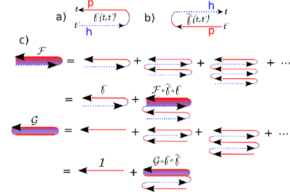
Figure 1: (Color online) a) The coherence function $\gamma(t,t^{\prime})$ describes the local probability amplitude for conversion of a hole (dotted line) at time $t^{\prime}$ to a particle (full line) at time $t$. For retarded functions $t>t^{\prime}$, and for advanced functions $t<t^{\prime}$. b) The corresponding local amplitude for conversion of a particle at time $t^{\prime}$ into a hole at time $t$ is described by the coherence function $\tilde{\gamma}(t,t^{\prime})$. c) Diagrammatic representation of Eqs. (17) and (21).

The numerical solution of the (non-linear) system of Eqs. (1) and (2) is greatly simplified by using a convenient parameterization of the Green functions in terms of retarded and advanced coherence functions $\gamma^{{\scriptscriptstyle\rm R,A}}$, $\tilde{\gamma}^{{\scriptscriptstyle\rm R,A}}$, and distribution functions $x$, $\tilde{x}$.eschrig97 ; eschrig99 ; eschrig00 ; eschrig04 The coherence functions are a generalization of the so-called Riccati amplitudesnagato93 ; schopohl95 to non-equilibrium situations. Using a projector formalism as described in Appendices B and  C we can write the retarded and advanced Green’s functions [here the upper (lower) sign corresponds to retarded (advanced)] as

$$\hat{g}^{{\scriptscriptstyle\rm R,A}} = \mp\,2\pi i\,\left(\begin{array}[]{cc}\;\;\,{\cal G}&\;\;\,{\cal F}\\ -\tilde{\cal F}&-\tilde{\cal G}\end{array}\right)^{\!\!\!{\scriptscriptstyle\rm R,A}}\pm i\pi\hat{\tau}_{3},$$ (16)

with the parameterizationeschrig97

$${\cal G} = ({\it 1}-\gamma{\circ}\tilde{\gamma})^{-1},\quad{\cal F}=({\it 1}-\gamma{\circ}\tilde{\gamma})^{-1}{\circ}\gamma,$$ (17)

$$\tilde{\cal G} = ({\it 1}-\tilde{\gamma}{\circ}\gamma)^{-1},\quad\tilde{\cal F}=({\it 1}-\tilde{\gamma}{\circ}\gamma)^{-1}{\circ}\tilde{\gamma}.$$ (18)

The inverse is defined via the $\circ$-product,

$$(\ldots)^{-1}{\circ}(\ldots)=(\ldots){\circ}(\ldots)^{-1}={\it 1},$$ (19)

with the unit element ${\it 1}$ (see Appendix A). Obviously, we can calculate the coherence functions from

$$\gamma={\cal G}^{-1}{\circ}{\cal F}={\cal F}{\circ}\tilde{\cal G}^{-1},\quad\tilde{\gamma}=\tilde{\cal G}^{-1}{\circ}\tilde{\cal F}=\tilde{\cal F}{\circ}{\cal G}^{-1}.\quad$$ (20)

In order to obtain a diagrammatic representation we re-formulate the problem in terms of Dyson equations

$${\cal G} = {\it 1}+{\cal G}{\circ}\gamma{\circ}\tilde{\gamma},\quad{\cal F}=\gamma+{\cal F}{\circ}\tilde{\gamma}{\circ}\gamma,$$ (21)

$$\tilde{\cal G} = {\it 1}+\tilde{\cal G}{\circ}\tilde{\gamma}{\circ}\gamma,\quad\tilde{\cal F}=\tilde{\gamma}+\tilde{\cal F}{\circ}\gamma{\circ}\tilde{\gamma}.$$ (22)

In Fig. 1 the corresponding diagrammatic expansion is shown. Here, and in the following, we adopt and extend a diagrammatic notation by Löfwander, Zhao and Sauls.lofwander02 ; zhao07 ; zhao08 The quantity ${\cal G}$ describes the local spectral amplitude of a particle-like excitation in the presence of a condensate. This amplitude is renormalized from its normal state value $\delta(t-t^{\prime})$ due to multiple virtual Andreev scattering processes that take place in the presence of an off-diagonal complex condensate field ${\it\Delta}$. The same holds for hole-like excitations, described by the quantity $\tilde{\cal G}$. The “anomalous” propagators ${\cal F}$ and $\tilde{\cal F}$ result from the local coherence amplitudes for particle-hole conversion, $\gamma$, and for hole-particle conversion, $\tilde{\gamma}$, again by taking into account renormalization due to multiple virtual Andreev processes. For small superconducting amplitudes (e.g. near $T_{\rm c}$) the anomalous propagators coincide with the coherence amplitudes.

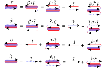
Figure 2: (Color online) Identities that hold between the six quantities ${\cal F}$, $\tilde{\cal F}$, ${\cal G}$, $\tilde{\cal G}$, $\gamma$, and $\tilde{\gamma}$ as defined in Eqs. (17)-(18).

The four functions ${\cal F}$, $\tilde{\cal F}$, ${\cal G}$ and $\tilde{\cal G}$ are inter-related via $\gamma$ and $\tilde{\gamma}$, and a number of identities hold that are shown in Fig. 2 diagrammatically.

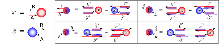
Figure 3: (Color online) The distribution functions $x$ and $\tilde{x}$ (left) connect incoming advanced and outgoing retarded propagators. The Keldysh components ${\cal X}^{{\scriptscriptstyle\rm K}}$, $\tilde{\cal X}^{{\scriptscriptstyle\rm K}}$, ${\cal Y}^{{\scriptscriptstyle\rm K}}$, and $\tilde{\cal Y}^{{\scriptscriptstyle\rm K}}$ are shown in a diagrammatic representation of Eqs. (33)-(36). “${\rm R}$” and “${\rm A}$” refer to “retarded” and “advanced”. The particle distribution function $x$ and hole distribution function $\tilde{x}$ are coherently mixed due to multiple coherent Andreev scattering events with amplitudes given by the renormalized quantities ${\cal G}$, $\tilde{\cal G}$, ${\cal F}$, and $\tilde{\cal F}$ that are sums of terms shown in Fig. 1.

Although the coherence functions $\gamma$ and $\tilde{\gamma}$ are sufficient to describe the retarded and advanced Green’s functions, the quantities in Eqs. (21)-(22) allow for an effective formulation of boundary conditions (see below). The Keldysh part of the propagator can be formulated in terms of these and a suitable distribution function for particle-like and hole-like excitations, respectively, in the following way,

$$\hat{g}^{{\scriptscriptstyle\rm K}}\equiv-2\pi i\left(\begin{array}[]{cc}\;\;\,{\cal X}&\;\;\,{\cal Y}\\ \tilde{\cal Y}&\tilde{\cal X}\end{array}\right)^{\!\!\!{\scriptscriptstyle\rm K}}$$ (25)

$$=-2\pi i\left(\begin{array}[]{cc}\;\;\,{\cal G}&\;\;\,{\cal F}\\ -\tilde{\cal F}&-\tilde{\cal G}\end{array}\right)^{\!\!\!{\scriptscriptstyle\rm R}}{\circ}\left(\begin{array}[]{cc}x&0\\ 0&\tilde{x}\end{array}\right){\circ}\left(\begin{array}[]{cc}\;\;\,{\cal G}&\;\;\,{\cal F}\\ -\tilde{\cal F}&-\tilde{\cal G}\end{array}\right)^{\!\!\!{\scriptscriptstyle\rm A}}.$$ (32)

Making use of the identities in Fig. 2, we can further use that ${\cal X}^{{\scriptscriptstyle\rm K}}={\cal G}^{{\scriptscriptstyle\rm R}}{\circ}x{\circ}{\cal G}^{{\scriptscriptstyle\rm A}}-{\cal F}^{{\scriptscriptstyle\rm R}}{\circ}\tilde{x}{\circ}\tilde{\cal F}^{{\scriptscriptstyle\rm A}}={\cal G}^{{\scriptscriptstyle\rm R}}{\circ}(x-\gamma^{{\scriptscriptstyle\rm R}}{\circ}\tilde{x}{\circ}\tilde{\gamma}^{{\scriptscriptstyle\rm A}}){\circ}{\cal G}^{{\scriptscriptstyle\rm A}}$ and similarly for the other components, which gives

$${\cal X}^{{\scriptscriptstyle\rm K}} = {\cal G}^{{\scriptscriptstyle\rm R}}{\circ}(x-\gamma^{{\scriptscriptstyle\rm R}}{\circ}\tilde{x}{\circ}\tilde{\gamma}^{{\scriptscriptstyle\rm A}}){\circ}{\cal G}^{{\scriptscriptstyle\rm A}},$$ (33)

$${\cal Y}^{{\scriptscriptstyle\rm K}} = {\cal G}^{{\scriptscriptstyle\rm R}}{\circ}(x{\circ}\gamma^{{\scriptscriptstyle\rm A}}-\gamma^{{\scriptscriptstyle\rm R}}{\circ}\tilde{x}){\circ}\tilde{\cal G}^{{\scriptscriptstyle\rm A}},$$ (34)

$$\tilde{\cal X}^{{\scriptscriptstyle\rm K}} = \tilde{\cal G}^{{\scriptscriptstyle\rm R}}{\circ}(\tilde{x}-\tilde{\gamma}^{{\scriptscriptstyle\rm R}}{\circ}x{\circ}\gamma^{{\scriptscriptstyle\rm A}}){\circ}\tilde{\cal G}^{{\scriptscriptstyle\rm A}},$$ (35)

$$\tilde{\cal Y}^{{\scriptscriptstyle\rm K}} = \tilde{\cal G}^{{\scriptscriptstyle\rm R}}{\circ}(\tilde{x}{\circ}\tilde{\gamma}^{{\scriptscriptstyle\rm A}}-\tilde{\gamma}^{{\scriptscriptstyle\rm R}}{\circ}x){\circ}{\cal G}^{{\scriptscriptstyle\rm A}}.$$ (36)

The Keldysh amplitudes ${\cal X}$, $\tilde{\cal X}$, ${\cal Y}$, and $\tilde{\cal Y}$ are shown in a diagrammatic representation in Fig. 3. Note that for the Keldysh components we need to keep track of retarded and advanced coherence functions. As advanced functions propagate backward in time, their group velocity is reversed. Advanced propagators can be described as usual by the particle-antiparticle paradigm, that in the present case is equivalent to a particle-hole transformation as described in Appendix G. In drawing diagrams we prefer to keep the particle picture instead of introducing antiparticles (which would reverse the arrows and turn them into hole propagators with opposite energy).

We stress that there are no diagrams with more than one $x$ or $\tilde{x}$ vertex, as no retarded propagator can enter either of them, and no advanced propagator can emerge from them. As a result, the structure of the equations for ${\cal X}$, $\tilde{\cal X}$, ${\cal Y}$, and $\tilde{\cal Y}$ formally corresponds to that of a linear response with a perturbation that switches from retarded to advanced (in fact, the linear response theory for retarded and advanced coherence functions has many formal similarities with the Keldysh part of the transport theory,eschrig99 see also Appendix E).

II.1.1 Alternative distribution functions

Other definitions for distribution functions have been introduced in the literature. We discuss the issue of the various possibilities in defining distribution functions and their relation with each other in detail in Appendix D. The distribution functions $h$ introduced by Larkin and Ovchinnikov larkin68 ; Larkin86 and $F$ introduced by Shelankov shelankov85 are related to the distribution functions $x$ and $\tilde{x}$ by

$$x = F-\gamma^{{\scriptscriptstyle\rm R}}{\circ}F{\circ}\tilde{\gamma}^{{\scriptscriptstyle\rm A}}=h+\gamma^{{\scriptscriptstyle\rm R}}{\circ}\tilde{h}{\circ}\tilde{\gamma}^{{\scriptscriptstyle\rm A}}\;,$$

$$\tilde{x} = \tilde{F}-\tilde{\gamma}^{{\scriptscriptstyle\rm R}}{\circ}\tilde{F}{\circ}\gamma^{{\scriptscriptstyle\rm A}}=\tilde{h}+\tilde{\gamma}^{{\scriptscriptstyle\rm R}}{\circ}h{\circ}\gamma^{{\scriptscriptstyle\rm A}}.$$ (37)

Series expansions for the inverses can be obtained by iteration,cuevas06 for example

$$F=\sum_{n=0}^{\infty}(\gamma^{{\scriptscriptstyle\rm R}})^{n}{\circ}x{\circ}(\tilde{\gamma}^{{\scriptscriptstyle\rm A}})^{n}$$ (38)

with $(\ldots)^{n}=(\ldots)^{n-1}{\circ}(\ldots)$, and

$$h=\sum_{n=0}^{\infty}(\gamma^{{\scriptscriptstyle\rm R}}\tilde{\gamma}^{{\scriptscriptstyle\rm R}})^{n}{\circ}(x-\gamma^{{\scriptscriptstyle\rm R}}{\circ}\tilde{x}{\circ}\tilde{\gamma}^{{\scriptscriptstyle\rm A}}){\circ}(\gamma^{{\scriptscriptstyle\rm A}}\tilde{\gamma}^{{\scriptscriptstyle\rm A}})^{n}.$$ (39)

In equilibrium,

$$h_{\rm eq}=F_{\rm eq}=\tanh\frac{\epsilon}{2T}=-\tilde{F}_{\rm eq}=-\tilde{h}_{\rm eq}$$ (40)

holds. The advantages of the functions $x$ and $\tilde{x}$ are that the transport equations take their simplest form,eschrig97 their numerical evaluation is easier, they simplify considerably time-dependent problems,eschrig97 ; eschrig99 ; cuevas06 and as we will show below, they allow for an effective handling of the boundary conditions.

II.2 Transport equations

The central equations that govern the transport phenomena have been derived in Ref. eschrig97 ; eschrig99 ; eschrig00 . The transport equation for the coherence functions $\gamma(\epsilon,{\mbox{\boldmath$p$}}_{\rm F},{\mbox{\boldmath$R$}},t)$ and $\tilde{\gamma}(\epsilon,{\mbox{\boldmath$p$}}_{\rm F},{\mbox{\boldmath$R$}},t)$ are given by

$$(i\hbar\,{\mbox{\boldmath$v$}}_{\rm F}\!\cdot\!\mbox{\boldmath$\nabla$}+2\epsilon)\gamma^{{\scriptscriptstyle\rm R,A}}=[\gamma{\circ}{\,\tilde{\!{\it\Delta}}}{\circ}\gamma+{\it\Sigma}{\circ}\gamma-\gamma{\circ}{\,\tilde{\!{\it\Sigma}}}-{\it\Delta}]^{{\scriptscriptstyle\rm R,A}},$$

$$(i\hbar\,{\mbox{\boldmath$v$}}_{\rm F}\!\cdot\!\mbox{\boldmath$\nabla$}-2\epsilon)\tilde{\gamma}^{{\scriptscriptstyle\rm R,A}}=[\tilde{\gamma}{\circ}{\it\Delta}{\circ}\tilde{\gamma}+{\,\tilde{\!{\it\Sigma}}}{\circ}\tilde{\gamma}-\tilde{\gamma}{\circ}{\it\Sigma}-{\,\tilde{\!{\it\Delta}}}]^{{\scriptscriptstyle\rm R,A}}.$$

(41)

For the distribution functions $x(\epsilon,{\mbox{\boldmath$p$}}_{\rm F},{\mbox{\boldmath$R$}},t)$ and $\tilde{x}(\epsilon,{\mbox{\boldmath$p$}}_{\rm F},{\mbox{\boldmath$R$}},t)$ the transport equations read

$$(i\hbar\,{\mbox{\boldmath$v$}}_{\rm F}\!\cdot\!\mbox{\boldmath$\nabla$}+i\hbar\,\partial_{t})x-[\gamma{\circ}{\,\tilde{\!{\it\Delta}}}+{\it\Sigma}]^{{\scriptscriptstyle\rm R}}{\circ}x-x{\circ}[{\it\Delta}{\circ}\tilde{\gamma}-{\it\Sigma}]^{{\scriptscriptstyle\rm A}}$$

$$\qquad=-\gamma^{{\scriptscriptstyle\rm R}}{\circ}{\,\tilde{\!{\it\Sigma}}}^{{\scriptscriptstyle\rm K}}{\circ}\tilde{\gamma}^{{\scriptscriptstyle\rm A}}+{\it\Delta}^{{\scriptscriptstyle\rm K}}{\circ}\tilde{\gamma}^{{\scriptscriptstyle\rm A}}+\gamma^{{\scriptscriptstyle\rm R}}{\circ}{\,\tilde{\!{\it\Delta}}}^{{\scriptscriptstyle\rm K}}-{\it\Sigma}^{{\scriptscriptstyle\rm K}},$$ (42)

$$(i\hbar\,{\mbox{\boldmath$v$}}_{\rm F}\!\cdot\!\mbox{\boldmath$\nabla$}-i\hbar\,\partial_{t})\tilde{x}-[\tilde{\gamma}{\circ}{\it\Delta}+{\,\tilde{\!{\it\Sigma}}}]^{{\scriptscriptstyle\rm R}}{\circ}\tilde{x}-\tilde{x}{\circ}[{\,\tilde{\!{\it\Delta}}}{\circ}\gamma-{\,\tilde{\!{\it\Sigma}}}]^{{\scriptscriptstyle\rm A}}$$

$$\qquad=-\tilde{\gamma}^{{\scriptscriptstyle\rm R}}{\circ}{\it\Sigma}^{{\scriptscriptstyle\rm K}}{\circ}\gamma^{{\scriptscriptstyle\rm A}}+{\,\tilde{\!{\it\Delta}}}^{{\scriptscriptstyle\rm K}}{\circ}\gamma^{{\scriptscriptstyle\rm A}}+\tilde{\gamma}^{{\scriptscriptstyle\rm R}}{\circ}{\it\Delta}^{{\scriptscriptstyle\rm K}}-{\,\tilde{\!{\it\Sigma}}}^{{\scriptscriptstyle\rm K}}.$$ (43)

In Appendix E we discuss properties of the solutions of these equations, and equivalent formulations in terms of integral equations.

An important property of the set of equations (II.2)-(II.2) is their invariance with respect to gauge transformations. There are two types of gauge transformations that are important, and that are very different in nature. We discuss this issue in Appendix F. The first type is the usual gauge invariance that links the phase of the coherence functions with the electromagnetic potentials. The second type leaves retarded and advanced quantities invariant and affects only the distribution functions $x$ and $\tilde{x}$ and the Keldysh part of the self energies. It leads to a certain freedom for the choice of the distribution functions (several choices have been mentioned above). In particular, when a reference system is present, distribution functions can be defined with respect to those of the reference system. They are then called “anomalous”,footanom and vanish in the reference system. This is particularly useful for situations when a system is coupled to a reservoir.

II.2.1 Homogeneous equilibrium solution

In the case that both ${\cal E}^{{\scriptscriptstyle\rm R,A}}=\epsilon-({\it\Sigma}^{{\scriptscriptstyle\rm R,A}}-{\,\tilde{\!{\it\Sigma}}}^{{\scriptscriptstyle\rm R,A}})/2$ and $[{\it\Delta}{\,\tilde{\!{\it\Delta}}}]^{\scriptscriptstyle\rm R,A}$ are diagonal in spin space, the homogeneous solutions for the coherence functions in equilibrium can be written as,

$$\gamma^{{\scriptscriptstyle\rm R,A}}_{\rm h,eq}=-\left[\frac{{\it\Delta}}{{\cal E}\pm i\sqrt{-{\it\Delta}{\,\tilde{\!{\it\Delta}}}-{\cal E}^{2}}}\right]^{{\scriptscriptstyle\rm R,A}}$$ (44)

where the upper (lower) sign holds for the retarded (advanced) functions. For a singlet superconductor in the clean limit $[{\it\Delta}{\,\tilde{\!{\it\Delta}}}]^{{\scriptscriptstyle\rm R,A}}=-|{\it\Delta}|^{2}$. In the presence of a constant superflow with momentum ${\mbox{\boldmath$p$}}_{s}$ one has to replace $\epsilon$ by $\epsilon-{\mbox{\boldmath$v$}}_{\rm F}\cdot{\mbox{\boldmath$p$}}_{s}$.

For the distribution function in equilibrium one obtains

$$x_{\rm h,eq}=(1-\gamma^{{\scriptscriptstyle\rm R}}\tilde{\gamma}^{{\scriptscriptstyle\rm A}})\tanh(\frac{\epsilon}{2T}).$$ (45)

Note that $\tilde{\gamma}^{{\scriptscriptstyle\rm A}}=(\gamma^{{\scriptscriptstyle\rm R}})^{\dagger}$ (see Appendix G).

II.2.2 General solution for homogeneous self energies

For homogeneous self energies we can express the solutions $\gamma^{{\scriptscriptstyle\rm R,A}}(\rho)$ along a certain trajectory with path variable $\rho$ (defined by the trajectory parameterization ${\mbox{\boldmath$R$}}={\mbox{\boldmath$R$}}_{0}+\rho{\mbox{\boldmath$v$}}_{\rm F}$), for a given initial value $\gamma^{{\scriptscriptstyle\rm R,A}}(0)=\gamma^{{\scriptscriptstyle\rm R,A}}_{0}$, in terms of the homogeneous solution $\gamma^{{\scriptscriptstyle\rm R,A}}_{\rm h}$ that satisfies

$$[\gamma_{\rm h}{\circ}{\,\tilde{\!{\it\Delta}}}{\circ}\gamma_{\rm h}-E{\circ}\gamma_{\rm h}+\gamma_{\rm h}{\circ}\tilde{E}-{\it\Delta}]^{{\scriptscriptstyle\rm R,A}}=0,$$ (46)

where $E^{{\scriptscriptstyle\rm R,A}}=\epsilon-{\it\Sigma}^{{\scriptscriptstyle\rm R,A}}$, $\tilde{E}^{{\scriptscriptstyle\rm R,A}}=-\epsilon-{\,\tilde{\!{\it\Sigma}}}^{{\scriptscriptstyle\rm R,A}}$. Defining ${\it\Omega}^{{\scriptscriptstyle\rm R,A}}_{1}=[E-\gamma_{\rm h}{\circ}{\,\tilde{\!{\it\Delta}}}]^{\scriptscriptstyle\rm R,A}$ and ${\it\Omega}^{{\scriptscriptstyle\rm R,A}}_{2}=[\tilde{E}+{\,\tilde{\!{\it\Delta}}}{\circ}\gamma_{\rm h}]^{\scriptscriptstyle\rm R,A}$, and using the relations of Appendix E.1, it follows as

$$\gamma^{{\scriptscriptstyle\rm R,A}}(\rho)=\left[\gamma_{\rm h}+e^{i\rho{\it\Omega}_{1}}{\circ}\delta_{0}{\circ}\big{\{}e^{i\rho{\it\Omega}_{2}}+C(\rho){\circ}\delta_{0}\big{\}}^{-1}\right]^{\scriptscriptstyle\rm R,A},$$ (47)

with $\delta^{\scriptscriptstyle\rm R,A}_{0}=\left[\gamma_{0}-\gamma_{\rm h}\right]^{\scriptscriptstyle\rm R,A}$ and

$$C^{\scriptscriptstyle\rm R,A}(\rho) = \left[C_{0}{\circ}e^{i\rho{\it\Omega}_{1}}-e^{i\rho{\it\Omega}_{2}}{\circ}C_{0}\right]^{\scriptscriptstyle\rm R,A}$$ (48)

where $C_{0}^{\scriptscriptstyle\rm R,A}$ is the solution of the equation

$$[C_{0}{\circ}{\it\Omega}_{1}-{\it\Omega}_{2}{\circ}C_{0}]^{\scriptscriptstyle\rm R,A}={\,\tilde{\!{\it\Delta}}}^{{\scriptscriptstyle\rm R,A}}.$$ (49)

For equilibrium we have $E^{{\scriptscriptstyle\rm R,A}}=-\tilde{E}^{{\scriptscriptstyle\rm R,A}}\equiv{\cal E}^{\scriptscriptstyle\rm R,A}$, and if ${\cal E}^{{\scriptscriptstyle\rm R,A}}$ and $[{\it\Delta}{\,\tilde{\!{\it\Delta}}}]^{\scriptscriptstyle\rm R,A}$ are diagonal in spin space, then with ${\it\Omega}^{\scriptscriptstyle\rm R,A}_{1}=-{\it\Omega}^{\scriptscriptstyle\rm R,A}_{2}\equiv{\it\Omega}^{\scriptscriptstyle\rm R,A}$ the relation

$$\gamma^{{\scriptscriptstyle\rm R,A}}(\rho)=\left[\frac{\gamma_{0}{\it\Omega}+i\tan(\rho{\it\Omega})(E\gamma_{0}+{\it\Delta})}{{\it\Omega}-i\tan(\rho{\it\Omega})(E-\gamma_{0}{\,\tilde{\!{\it\Delta}}})}\right]^{\scriptscriptstyle\rm R,A}$$ (50)

follows, in agreement with Ref. kalenkov07, .

II.2.3 Equilibrium solution for sub-gap energies in the presence of an inhomogeneous order parameter in the clean limit

If we can neglect impurity scattering, and the system outside the scattering region is asymptotically homogeneous with gap ${\it\Delta}_{\rm h}$, then for sub-gap energies $|\epsilon|\leq|{\it\Delta}_{\rm h}|$ we can make some more general statments about the properties of the coherence amplitudes. In particular, if we e.g. consider a pure singlet pairing state, and if the order parameter is of the form ${\it\Delta}={\it\Delta}_{0}(\rho)e^{i\chi}i\sigma_{y}$ with spatially varying modulus ${\it\Delta}_{0}$ and spatially constant phase $\chi$, then, using the ansatz $\gamma^{{\scriptscriptstyle\rm R}}(\rho)=i\gamma_{0}^{\,}(\rho)e^{i[\chi+{\it\Psi}(\rho)]}\cdot i\sigma_{y}$ with real $\gamma_{0}^{\,}$ and ${\it\Psi}$, the equilibrium equations of motion along any fixed trajectory read

$$\frac{{\rm d}\gamma_{0}^{\,}}{{\rm d}\rho} = \;\;\,(1-\gamma_{0}^{2}){\it\Delta}_{0}\cos({\it\Psi})-0^{+}\gamma_{0}^{\,}$$ (51)

$$\gamma_{0}^{\,}\frac{{\rm d}{\it\Psi}}{{\rm d}\rho} = -(1+\gamma_{0}^{2}){\it\Delta}_{0}\sin({\it\Psi})+2\epsilon\gamma_{0}^{\,},$$ (52)

where $0^{+}$ is a positive infinitesimal. The first equation is stable only in direction of increasing $\rho$. Now, for the initial condition far away from the scatterer, for sub-gap energies $|\epsilon|\leq|{\it\Delta}_{\rm h}|$ the relation $\gamma_{0}^{\,}=1$ holds. Then, as Eq. 51 shows, this property will be preserved along the trajectory regardless of the spatial variation of ${\it\Delta}_{0}(\rho)$. That means, only the phase ${\it\Psi}$ of the coherence amplitude varies, and we have $\gamma^{{\scriptscriptstyle\rm R}}=ie^{i[\chi+{\it\Psi}(\rho)]}\cdot i\sigma_{y}$ with

$$\frac{{\rm d}{\it\Psi}(\rho)}{{\rm d}\rho} = -2{\it\Delta}_{0}(\rho)\sin\big{(}{\it\Psi}(\rho)\big{)}+2\epsilon$$ (53)

and initial condition ${\it\Psi}(\rho_{0})=0$. If $\epsilon=0$, then the coherence amplitude stays constant along the trajectory. Similarly, we obtain $\tilde{\gamma}^{{\scriptscriptstyle\rm R}}=-ie^{-i[\chi+{\,\tilde{\!{\it\Psi}}}(\rho)]}\cdot i\sigma_{y}$ with

$$\frac{{\rm d}{\,\tilde{\!{\it\Psi}}}(\rho)}{{\rm d}\rho} = 2{\it\Delta}_{0}(\rho)\sin\big{(}{\,\tilde{\!{\it\Psi}}}(\rho)\big{)}+2\epsilon.$$ (54)

For energies $|\epsilon|>|{\it\Delta}_{\rm h}|$ both the modulus and phase of $\gamma^{{\scriptscriptstyle\rm R}}$, $\tilde{\gamma}^{{\scriptscriptstyle\rm R}}$ vary in space. A similar consideration can be made for any unitary order parameter.

III Scattering Theory

We consider in the following a general quantum mechanical scattering problem that is characterized by incoming and outgoing Bloch wave solutions. We assume that the scattering region is localized in a certain space area, where we have in mind e.g. an interface, a surface, or an impurity. In quasiclassical context there will be trajectories that enter and leave the scattering region. Correspondingly we can define incoming solutions along each trajectory as those for which the group velocity is pointing towards the scattering region under consideration (the “scatterer”), and outgoing those for which the group velocity is pointing away. The projection of the group velocity on the Fermi momentum has one and the same sign for $\gamma^{{\scriptscriptstyle\rm R}}$, $\tilde{\gamma}^{{\scriptscriptstyle\rm A}}$, and $x$, and the opposite sign for $\tilde{\gamma}^{{\scriptscriptstyle\rm R}}$, $\gamma^{{\scriptscriptstyle\rm A}}$, and $\tilde{x}$. Correspondingly, these six objects for each trajectory always group into three incoming and three outgoing ones.

The scatterer will lead to a mixing between the trajectories that enter the scattering region. Depending on symmetry constraints, the possible number of scattering wave vectors might be drastically reduced, as for example is the case for conservation of parallel momentum at an atomically clean interface. In the latter case, for a single Fermi surface on each side of the interface, there will be mixing only between the incoming, reflected, transmitted trajectory, and a fourth trajectory that is reached by a process involving “crossed” Andreev reflection. In the case of a diffusive interface trajectories of all directions will be mixed with each other.

In order to distinguish incoming and outgoing directions we will adopt the notation of Ref. eschrig00, , that small case letters $\gamma^{{\scriptscriptstyle\rm R,A}}$, $\tilde{\gamma}^{{\scriptscriptstyle\rm R,A}}$, $x$, $\tilde{x}$ denote incoming quantities, and capital case letters ${\it\Gamma}^{{\scriptscriptstyle\rm R,A}}$, ${\,\tilde{\!{\it\Gamma}}}^{{\scriptscriptstyle\rm R,A}}$, $X$, $\tilde{X}$ denote outgoing quantities. As the quasiclassical Green’s function is parameterized by the momentum ${\mbox{\boldmath$p$}}_{\rm F}$, it is composed of both incoming and outgoing quantities. We may write the Keldysh matrix Green’s function as a functional of the four coherence functions and the two distribution functions. If the Fermi velocity points towards the scatterer, this functional dependence will be

$$\check{g}=\check{g}[\gamma^{{\scriptscriptstyle\rm R}},{\,\tilde{\!{\it\Gamma}}}^{{\scriptscriptstyle\rm R}},{\it\Gamma}^{{\scriptscriptstyle\rm A}},\tilde{\gamma}^{{\scriptscriptstyle\rm A}},x,\tilde{X}],$$ (55)

and for the case that the Fermi velocity points away from the scatterer, it is

$$\check{g}=\check{g}[{\it\Gamma}^{{\scriptscriptstyle\rm R}},\tilde{\gamma}^{{\scriptscriptstyle\rm R}},\gamma^{{\scriptscriptstyle\rm A}},{\,\tilde{\!{\it\Gamma}}}^{{\scriptscriptstyle\rm A}},X,\tilde{x}].$$ (56)

Usually the potentials in a scattering region vary on a energy scale large compared to the superconducting gap or the temperature. In this case, it is sufficient to know the normal state scattering matrices for particle-like excitations, denoted by $S$ with elements $S({\mbox{\boldmath$p$}}_{\rm F}\leftarrow{\mbox{\boldmath$p$}}_{\rm F}^{\prime})$, and for hole-like excitations, denoted by $\tilde{S}$ with elements $\tilde{S}({\mbox{\boldmath$p$}}_{\rm F}^{\prime}\leftarrow{\mbox{\boldmath$p$}}_{\rm F})$, that connect outgoing with incoming quasiparticles on trajectories parameterized by the Fermi momenta ${\mbox{\boldmath$p$}}_{\rm F}$ and ${\mbox{\boldmath$p$}}_{\rm F}^{\prime}$.footscatt The scattering matrix in particle-hole space reads

$$\hat{\mbox{\boldmath$S$}}=\left(\begin{array}[]{cc}{\mbox{\boldmath$S$}}&0\\ 0&{\tilde{\mbox{\boldmath$S$}}}^{\dagger}\end{array}\right)\qquad\hat{\mbox{\boldmath$S$}}^{\dagger}=\left(\begin{array}[]{cc}{\mbox{\boldmath$S$}}^{\dagger}&0\\ 0&{\tilde{\mbox{\boldmath$S$}}}\end{array}\right).$$ (61)

In order to reduce the amount of notation we will in the following label trajectories with the Fermi velocity pointing away from the scatterer simply by $k$, $k^{\prime}$, $k_{1}$ etc, and trajectories with the Fermi velocity pointing towards the scatterer by $p$, $p^{\prime}$, $p_{1}$ etc, thus omitting the vector notation. It is understood that those labels are from the set of Fermi momenta associated with all the trajectories that overlap with the scattering region. As for the discussion in this chapter the dynamical variables (energy, time) enter only as parameters, we will suppress the dependence on these. We assume for the scattering problem that the spatial coordinate $R$ on each trajectory entering or leaving the scattering region is sufficiently far from the scatterer in order that the scattered waves have taken their asymptotic form, but sufficiently close to neglect spatial variations on the scale of the coherence length in the scattering region, and we will suppress these spatial coordinates in this chapter as well. The scattering problem will thus be fully characterized by the set of $k$ and $p$ values associated with all involved trajectories. In a centro-symmetric system (or a non-centrosymmetric system with time reversal symmetry), for each $k$ value there will also be the trajectory with the opposite direction $p=-k$.

It is our task to express the set of outgoing coherence and distribution functions ${\it\Gamma}^{{\scriptscriptstyle\rm R}}_{k}$,${\,\tilde{\!{\it\Gamma}}}^{{\scriptscriptstyle\rm R}}_{p}$, ${\it\Gamma}^{{\scriptscriptstyle\rm A}}_{p}$,${\,\tilde{\!{\it\Gamma}}}^{{\scriptscriptstyle\rm A}}_{k}$, $X_{k}$ $\tilde{X}_{p}$ by the incoming ones $\gamma^{{\scriptscriptstyle\rm R}}_{p}$,$\tilde{\gamma}^{{\scriptscriptstyle\rm R}}_{k}$, $\gamma^{{\scriptscriptstyle\rm A}}_{k}$,$\tilde{\gamma}^{{\scriptscriptstyle\rm A}}_{p}$, $x_{p}$ $\tilde{x}_{k}$ for a given scattering matrix $S_{kp}$ (the scattering matrix $\tilde{S}_{pk}$ for hole-like excitations is related to that for particle-like excitations by the particle-hole conjugation symmetry).

III.1 Elementary interface Andreev scattering events

The central objects for the formulation of boundary conditions for the coherence functions and distribution functions are the following quantities, that express an elementary scattering event,

$$[\gamma^{\prime}_{kk^{\prime}}]^{{\scriptscriptstyle\rm R}} = [\sum_{p}S_{kp}{\circ}\gamma_{p}{\circ}\tilde{S}_{pk^{\prime}}]^{{\scriptscriptstyle\rm R}},$$ (62)

$$[\gamma^{\prime}_{pp^{\prime}}]^{{\scriptscriptstyle\rm A}} = [\sum_{k}S_{pk}{\circ}\gamma_{k}{\circ}\tilde{S}_{kp^{\prime}}]^{{\scriptscriptstyle\rm A}},$$ (63)

$$x^{\prime}_{kk^{\prime}} = \sum_{p}S^{{\scriptscriptstyle\rm R}}_{kp}{\circ}x_{p}{\circ}S^{{\scriptscriptstyle\rm A}}_{pk^{\prime}},$$ (64)

together with the respective particle-hole conjugated quantities,

$$[\tilde{\gamma}^{\prime}_{pp^{\prime}}]^{{\scriptscriptstyle\rm R}} = [\sum_{k}\tilde{S}_{pk}{\circ}\tilde{\gamma}_{k}{\circ}S_{kp^{\prime}}]^{{\scriptscriptstyle\rm R}}$$ (65)

$$[\tilde{\gamma}^{\prime}_{kk^{\prime}}]^{{\scriptscriptstyle\rm A}} = [\sum_{p}\tilde{S}_{kp}{\circ}\tilde{\gamma}_{p}{\circ}S_{pk^{\prime}}]^{{\scriptscriptstyle\rm A}}$$ (66)

$$\tilde{x}^{\prime}_{pp^{\prime}} = \sum_{k}\tilde{S}^{{\scriptscriptstyle\rm R}}_{pk}{\circ}\tilde{x}_{k}{\circ}\tilde{S}^{{\scriptscriptstyle\rm A}}_{kp^{\prime}}.$$ (67)

As we will show below, the scattering matrices enter the boundary conditions only in terms of these quantities. This allows for a compact matrix notation. For example, we can re-formulate boundary conditions for spin active interfaces that are known in literature,fogelstrom00 ; zhao04 in a rather compact way. Importantly, a straightforward generalization of these boundary conditions to multiple bands, to disordered interfaces, to strongly spin polarized ferromagnets, to strongly spin-orbit split bands, and to the general scattering problem from a target is possible. For equilibrium we recover also the results by Shelankov and Ozana,ozana00 that were obtained by a similar procedure. In order to switch to a compact matrix notation, we introduce the diagonal matrices

$$\gamma_{kk^{\prime}}^{{\scriptscriptstyle\rm R}} = \gamma_{k}^{{\scriptscriptstyle\rm R}}\,\delta_{kk^{\prime}},\quad\gamma_{pp^{\prime}}^{{\scriptscriptstyle\rm A}}=\gamma_{p}^{{\scriptscriptstyle\rm A}}\,\delta_{pp^{\prime}},\quad x_{kk^{\prime}}=x_{k}\,\delta_{kk^{\prime}},\qquad$$ (68)

$$\tilde{\gamma}_{pp^{\prime}}^{{\scriptscriptstyle\rm R}} = \tilde{\gamma}_{p}^{{\scriptscriptstyle\rm R}}\,\delta_{pp^{\prime}},\quad\tilde{\gamma}_{kk^{\prime}}^{{\scriptscriptstyle\rm A}}=\tilde{\gamma}_{k}^{{\scriptscriptstyle\rm A}}\,\delta_{kk^{\prime}},\quad\tilde{x}_{pp^{\prime}}=\tilde{x}_{p}\,\delta_{pp^{\prime}}.$$ (69)

With this, we can write the elementary scattering events as

$$[\mbox{ \boldmath$\gamma$}^{\prime}]^{{\scriptscriptstyle\rm R,A}} = [\mbox{ \boldmath$S$}{\circ}\mbox{ \boldmath$\gamma$}{\circ}\mbox{ \boldmath$\tilde{S}$}]^{{\scriptscriptstyle\rm R,A}},\mbox{ \boldmath$x$}^{\prime}=\mbox{ \boldmath$S$}^{{\scriptscriptstyle\rm R}}{\circ}\mbox{ \boldmath$x$}{\circ}\mbox{ \boldmath$S$}^{{\scriptscriptstyle\rm A}},\qquad$$ (70)

$$[\mbox{ \boldmath$\tilde{\gamma}$}^{\prime}]^{{\scriptscriptstyle\rm R,A}} = [\mbox{ \boldmath$\tilde{S}$}{\circ}\mbox{ \boldmath$\tilde{\gamma}$}{\circ}\mbox{ \boldmath$S$}]^{{\scriptscriptstyle\rm R,A}},\mbox{ \boldmath$\tilde{x}$}^{\prime}=\mbox{ \boldmath$\tilde{S}$}^{{\scriptscriptstyle\rm R}}{\circ}\mbox{ \boldmath$\tilde{x}$}{\circ}\mbox{ \boldmath$\tilde{S}$}^{{\scriptscriptstyle\rm A}}.\qquad$$ (71)

Figure 4: (Color online) Diagrammatic symbols for the elementary scattering events described by Eqs. (70)-(71). $p$ and $h$ refers to “particle” and “hole”, and “${\rm R}$” and “${\rm A}$” to “retarded” and “advanced”. A sum over internal variables according to Eqs. (62)-(64) is implied.

In Fig. 4 we show these scattering events in diagrammatic form. We note that the retarded and advanced scattering matrices are related by fundamental symmetry,

$$\mbox{ \boldmath$S$}^{{\scriptscriptstyle\rm A}}=[\mbox{ \boldmath$S$}^{{\scriptscriptstyle\rm R}}]^{\dagger},\quad\mbox{ \boldmath$\tilde{S}$}^{{\scriptscriptstyle\rm A}}=[\mbox{ \boldmath$\tilde{S}$}^{{\scriptscriptstyle\rm R}}]^{\dagger},$$ (72)

which leads together with the symmetries in Appendix G to the symmetry relations

$$\,[\mbox{ \boldmath$\gamma$}^{\prime}]^{{\scriptscriptstyle\rm A}} = [\mbox{ \boldmath$\tilde{\gamma}$}^{\prime}]^{{\scriptscriptstyle\rm R}\dagger},\quad\mbox{ \boldmath$x$}^{\prime}=[\mbox{ \boldmath$x$}^{\prime}]^{\dagger},$$ (73)

$$\,[\mbox{ \boldmath$\tilde{\gamma}$}^{\prime}]^{{\scriptscriptstyle\rm A}} = [\mbox{ \boldmath$\gamma$}^{\prime}]^{{\scriptscriptstyle\rm R}\dagger},\quad\mbox{ \boldmath$\tilde{x}$}^{\prime}=[\mbox{ \boldmath$\tilde{x}$}^{\prime}]^{\dagger}.$$ (74)

III.2 Derivation of boundary conditions

III.2.1 Retarded Propagator

The anomalous functions ${\cal F}^{{\scriptscriptstyle\rm R}}$ are obtained from a sum over all virtual multiple Andreev scattering events that are accompanied by interface scattering. We consider first the set of retarded Green’s functions with directions $k$ that are directed away from the scatterer. In this case, the retarded propagator is given by

$$\hat{g}_{k}^{{\scriptscriptstyle\rm R}}=\hat{g}^{{\scriptscriptstyle\rm R}}_{k}[{\it\Gamma}^{{\scriptscriptstyle\rm R}},\tilde{\gamma}^{{\scriptscriptstyle\rm R}}].$$ (75)

We introduce effective interface coherence amplitudes as solutions of the equation

$$\,[{\cal F}_{kk^{\prime}}]^{{\scriptscriptstyle\rm R}} = \left[\gamma^{\prime}_{kk^{\prime}}+\sum_{k_{1}}{\cal F}_{kk_{1}}{\circ}\tilde{\gamma}_{k_{1}}{\circ}\gamma^{\prime}_{k_{1}k^{\prime}}\right]^{{\scriptscriptstyle\rm R}}.$$ (76)

Using a compact matrix notation, the solutions are

$$\,\mbox{ \boldmath$\cal F$}^{{\scriptscriptstyle\rm R}} = \left[\mbox{ \boldmath$\gamma$}^{\prime}{\circ}\left(\mbox{ \boldmath$1$}-\mbox{ \boldmath$\tilde{\gamma}$}{\circ}\mbox{ \boldmath$\gamma$}^{\prime}\right)^{-1}\right]^{{\scriptscriptstyle\rm R}},$$ (77)

where the inversion $\mbox{ \boldmath$Q$}^{-1}$ is defined via $\mbox{ \boldmath$Q$}{\circ}\mbox{ \boldmath$Q$}^{-1}=\mbox{ \boldmath$1$}$ with $1_{kk^{\prime}}=\delta_{kk^{\prime}}{\it 1}$. The diagrammatic representation of this expansion is shown in Fig. 5.

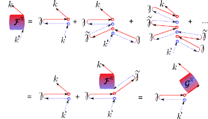
Figure 5: (Color online) Diagrammatic representation of Eq. (76) for the retarded functions. In the last line the identity (79) is shown diagrammatically, which defines the diagrammatic expansion for ${\cal G}^{{\scriptscriptstyle\rm R}}$. Summation over internal variables is implied.

We also define the corresponding particle-hole diagonal interface amplitude

$$\,\mbox{ \boldmath$\cal G$}^{{\scriptscriptstyle\rm R}} = \left[\left(\mbox{ \boldmath$1$}-\mbox{ \boldmath$\gamma$}^{\prime}{\circ}\mbox{ \boldmath$\tilde{\gamma}$}\right)^{-1}\right]^{{\scriptscriptstyle\rm R}}=1+\left[\mbox{ \boldmath$\cal F$}{\circ}\mbox{ \boldmath$\tilde{\gamma}$}\right]^{{\scriptscriptstyle\rm R}},$$ (78)

that is closely related to the function $\mbox{ \boldmath$\cal F$}^{{\scriptscriptstyle\rm R}}$ by

$$\,\mbox{ \boldmath$\cal F$}^{{\scriptscriptstyle\rm R}} = \left[\mbox{ \boldmath$\cal G$}{\circ}\mbox{ \boldmath$\gamma$}^{\prime}\right]^{{\scriptscriptstyle\rm R}}.$$ (79)

For the quasiclassical approximation only the component $k^{\prime}=k$ is relevant, as it contributes to the slowly varying envelope function of trajectory $k$, and we obtain

$${\cal G}^{{\scriptscriptstyle\rm R}}_{k} = {\cal G}^{{\scriptscriptstyle\rm R}}_{kk},\quad{\cal F}^{{\scriptscriptstyle\rm R}}_{k}={\cal F}^{{\scriptscriptstyle\rm R}}_{kk}\quad.$$ (80)

The remaining two retarded Green’s function matrix components are $\tilde{\cal G}^{{\scriptscriptstyle\rm R}}_{k}=[(\mbox{ \boldmath$1$}-\mbox{ \boldmath$\tilde{\gamma}$}{\circ}\mbox{ \boldmath$\gamma$}^{\prime})^{-1}]^{{\scriptscriptstyle\rm R}}_{kk}$ and $\tilde{\cal F}^{{\scriptscriptstyle\rm R}}_{k}=\tilde{\cal G}^{{\scriptscriptstyle\rm R}}_{k}{\circ}\tilde{\gamma}^{{\scriptscriptstyle\rm R}}_{k}$. According to section II.1, for the outgoing coherence functions the equation ${\cal F}^{\scriptscriptstyle\rm R}_{kk}={\it\Gamma}^{{\scriptscriptstyle\rm R}}_{k}+{\cal F}^{\scriptscriptstyle\rm R}_{kk}{\circ}\tilde{\gamma}^{{\scriptscriptstyle\rm R}}_{k}{\circ}{\it\Gamma}^{{\scriptscriptstyle\rm R}}_{k}=({\it 1}+{\cal F}^{\scriptscriptstyle\rm R}_{kk}{\circ}\tilde{\gamma}^{{\scriptscriptstyle\rm R}}_{k}){\circ}{\it\Gamma}^{{\scriptscriptstyle\rm R}}_{k}$ holds, which according to Eq. 78 is equal to ${\cal G}^{\scriptscriptstyle\rm R}_{kk}{\circ}{\it\Gamma}^{{\scriptscriptstyle\rm R}}_{k}$. Thus, we extract the outgoing coherence amplitudes from the solution of the equation

$${\cal G}^{{\scriptscriptstyle\rm R}}_{kk}{\circ}{\it\Gamma}^{{\scriptscriptstyle\rm R}}_{k\leftarrow k^{\prime}} = {\cal F}^{{\scriptscriptstyle\rm R}}_{kk^{\prime}},\quad{\it\Gamma}^{{\scriptscriptstyle\rm R}}_{k}={\it\Gamma}^{{\scriptscriptstyle\rm R}}_{k\leftarrow k}\quad.$$ (81)

The more general quantity ${\it\Gamma}^{{\scriptscriptstyle\rm R}}_{k\leftarrow k^{\prime}}$ that is introduced here will be needed below, e.g. in the transport equations for the distribution functions.

For the component ${\,\tilde{\!{\it\Gamma}}}^{{\scriptscriptstyle\rm R}}$ we must consider the retarded Green’s function for a direction $p$ towards the scatterer, as the group velocity of ${\,\tilde{\!{\it\Gamma}}}^{{\scriptscriptstyle\rm R}}$ is opposite to the direction of the momentum. The corresponding retarded propagator is given by,

$$\hat{g}^{{\scriptscriptstyle\rm R}}_{p}=\hat{g}^{{\scriptscriptstyle\rm R}}_{p}[\gamma^{{\scriptscriptstyle\rm R}},{\,\tilde{\!{\it\Gamma}}}^{{\scriptscriptstyle\rm R}}].$$ (82)

We obtain in complete analogy to the discussion above

$$\,\mbox{ \boldmath$\tilde{\cal F}$}^{{\scriptscriptstyle\rm R}} = \left[\mbox{ \boldmath$\tilde{\gamma}$}^{\prime}{\circ}\left(\mbox{ \boldmath$1$}-\mbox{ \boldmath$\gamma$}{\circ}\mbox{ \boldmath$\tilde{\gamma}$}^{\prime}\right)^{-1}\right]^{{\scriptscriptstyle\rm R}}=\left[\mbox{ \boldmath$\tilde{\cal G}$}{\circ}\mbox{ \boldmath$\tilde{\gamma}$}^{\prime}\right]^{{\scriptscriptstyle\rm R}},\quad$$ (83)

$$\,\mbox{ \boldmath$\tilde{\cal G}$}^{{\scriptscriptstyle\rm R}} = \left[\left(\mbox{ \boldmath$1$}-\mbox{ \boldmath$\tilde{\gamma}$}^{\prime}{\circ}\mbox{ \boldmath$\gamma$}\right)^{-1}\right]^{{\scriptscriptstyle\rm R}}=1+\left[\mbox{ \boldmath$\tilde{\cal F}$}{\circ}\mbox{ \boldmath$\gamma$}\right]^{{\scriptscriptstyle\rm R}},$$ (84)

from which we extract the outgoing coherence amplitude by solving the equation

$$\tilde{\cal G}^{{\scriptscriptstyle\rm R}}_{pp}{\circ}\tilde{\it\Gamma}^{{\scriptscriptstyle\rm R}}_{p\leftarrow p^{\prime}} = \tilde{\cal F}^{{\scriptscriptstyle\rm R}}_{pp^{\prime}},\quad\tilde{\it\Gamma}^{{\scriptscriptstyle\rm R}}_{p}=\tilde{\it\Gamma}^{{\scriptscriptstyle\rm R}}_{p\leftarrow p}\quad.$$ (85)

III.2.2 Advanced Propagator

For the advanced functions we need to take into account that they propagate backward in time. Thus, we consider for ${\it\Gamma}^{{\scriptscriptstyle\rm A}}$ the advanced Green’s function for a direction $p$ towards the scatterer,

$$\hat{g}^{{\scriptscriptstyle\rm A}}_{p}=\hat{g}^{{\scriptscriptstyle\rm A}}_{p}[{\it\Gamma}^{{\scriptscriptstyle\rm A}},\tilde{\gamma}^{{\scriptscriptstyle\rm A}}],$$ (86)

and for ${\,\tilde{\!{\it\Gamma}}}^{{\scriptscriptstyle\rm A}}$ for a direction $k$ away from the scatterer,

$$\hat{g}^{{\scriptscriptstyle\rm A}}_{k}=\hat{g}^{{\scriptscriptstyle\rm A}}_{k}[\gamma^{{\scriptscriptstyle\rm A}},{\,\tilde{\!{\it\Gamma}}}^{{\scriptscriptstyle\rm A}}].$$ (87)

The most convenient form of the corresponding equations is

$$\,\mbox{ \boldmath$\cal F$}^{{\scriptscriptstyle\rm A}} = \left[\mbox{ \boldmath$\gamma$}^{\prime}{\circ}\left(\mbox{ \boldmath$1$}-\mbox{ \boldmath$\tilde{\gamma}$}{\circ}\mbox{ \boldmath$\gamma$}^{\prime}\right)^{-1}\right]^{{\scriptscriptstyle\rm A}}=\left[\mbox{ \boldmath$\gamma$}^{\prime}{\circ}\mbox{ \boldmath$\tilde{\cal G}$}\right]^{{\scriptscriptstyle\rm A}},\quad$$ (88)

$$\,\mbox{ \boldmath$\tilde{\cal G}$}^{{\scriptscriptstyle\rm A}} = \left[\left(\mbox{ \boldmath$1$}-\mbox{ \boldmath$\tilde{\gamma}$}{\circ}\mbox{ \boldmath$\gamma$}^{\prime}\right)^{-1}\right]^{{\scriptscriptstyle\rm A}}=1+\left[\mbox{ \boldmath$\tilde{\gamma}$}{\circ}\mbox{ \boldmath$\cal F$}\right]^{{\scriptscriptstyle\rm A}},$$ (89)

with the the coherence amplitudes

$${\it\Gamma}^{{\scriptscriptstyle\rm A}}_{p^{\prime}\rightarrow p}{\circ}\tilde{\cal G}^{{\scriptscriptstyle\rm A}}_{pp} = {\cal F}^{{\scriptscriptstyle\rm A}}_{p^{\prime}p},\quad{\it\Gamma}^{{\scriptscriptstyle\rm A}}_{p}={\it\Gamma}^{{\scriptscriptstyle\rm A}}_{p\rightarrow p}\quad,$$ (90)

and

$$\,\mbox{ \boldmath$\tilde{\cal F}$}^{{\scriptscriptstyle\rm A}} = \left[\mbox{ \boldmath$\tilde{\gamma}$}^{\prime}{\circ}\left(\mbox{ \boldmath$1$}-\mbox{ \boldmath$\gamma$}{\circ}\mbox{ \boldmath$\tilde{\gamma}$}^{\prime}\right)^{-1}\right]^{{\scriptscriptstyle\rm A}}=\left[\mbox{ \boldmath$\tilde{\gamma}$}^{\prime}{\circ}\mbox{ \boldmath$\cal G$}\right]^{{\scriptscriptstyle\rm A}},$$ (91)

$$\,\mbox{ \boldmath$\cal G$}^{{\scriptscriptstyle\rm A}} = \left[\left(\mbox{ \boldmath$1$}-\mbox{ \boldmath$\gamma$}{\circ}\mbox{ \boldmath$\tilde{\gamma}$}^{\prime}\right)^{-1}\right]^{{\scriptscriptstyle\rm A}}=1+\left[\mbox{ \boldmath$\gamma$}{\circ}\mbox{ \boldmath$\tilde{\cal F}$}\right]^{{\scriptscriptstyle\rm A}},$$ (92)

with the the coherence amplitudes

$${\,\tilde{\!{\it\Gamma}}}^{{\scriptscriptstyle\rm A}}_{k^{\prime}\rightarrow k}{\circ}{\cal G}^{{\scriptscriptstyle\rm A}}_{kk} = \tilde{\cal F}^{{\scriptscriptstyle\rm A}}_{k^{\prime}k},\quad{\,\tilde{\!{\it\Gamma}}}^{{\scriptscriptstyle\rm A}}_{k}={\,\tilde{\!{\it\Gamma}}}^{{\scriptscriptstyle\rm A}}_{k\rightarrow k}\quad.$$ (93)

III.2.3 Keldysh Propagator

The corresponding expressions for the Keldysh components are obtained in a similar way. We perform a diagrammatic expansion of the Keldysh components in the elementary scattering events, using the fact that the vertices $x$ and $\tilde{x}$ can only occur once in each diagram (see end of section II.1). Thus, all renormalizations affect only the particle-hole conversion processes on either side of the $x$ and $\tilde{x}$ vertices. We consider first the Keldysh Green’s function for $k$ being directed away from the scatterer,

$$\hat{g}^{{\scriptscriptstyle\rm K}}_{k}=\hat{g}^{{\scriptscriptstyle\rm K}}_{k}[{\it\Gamma}^{{\scriptscriptstyle\rm R}},\tilde{\gamma}^{{\scriptscriptstyle\rm R}},\gamma^{{\scriptscriptstyle\rm A}},{\,\tilde{\!{\it\Gamma}}}^{{\scriptscriptstyle\rm A}},X,\tilde{x}],$$ (94)

for which the expansion, shown in Fig. 6a, gives

$$\mbox{ \boldmath$\cal X$}^{{\scriptscriptstyle\rm K}} = \mbox{ \boldmath$\cal G$}^{{\scriptscriptstyle\rm R}}{\circ}(\mbox{ \boldmath$x$}^{\prime}-{\mbox{ \boldmath$\gamma$}^{\prime}}^{{\scriptscriptstyle\rm R}}{\circ}\mbox{ \boldmath$\tilde{x}$}{\circ}{\mbox{ \boldmath$\tilde{\gamma}$}^{\prime}}^{{\scriptscriptstyle\rm A}}){\circ}\mbox{ \boldmath$\cal G$}^{{\scriptscriptstyle\rm A}}.$$ (95)

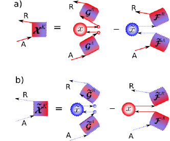
Figure 6: (Color online) Diagrammatic representation of Eqs. (95) and (98), using the identities in Eq. (79) and (83).

We obtain the distribution functions $X$ in terms of $\mbox{ \boldmath$\cal X$}^{{\scriptscriptstyle\rm K}}$ by

$${\cal G}_{kk}^{{\scriptscriptstyle\rm R}}{\circ}\left(X_{k}-{\it\Gamma}_{k}^{{\scriptscriptstyle\rm R}}{\circ}\tilde{x}_{k}{\circ}{\,\tilde{\!{\it\Gamma}}}_{k}^{{\scriptscriptstyle\rm A}}\right){\circ}\tilde{\cal G}_{kk}^{{\scriptscriptstyle\rm A}}={\cal X}^{{\scriptscriptstyle\rm K}}_{kk}\quad.$$ (96)

Similarly, considering the Keldysh Green’s function for $p$ being directed towards the scatterer,

$$\hat{g}^{{\scriptscriptstyle\rm K}}_{p}=\hat{g}^{{\scriptscriptstyle\rm K}}_{p}[\gamma^{{\scriptscriptstyle\rm R}},{\,\tilde{\!{\it\Gamma}}}^{{\scriptscriptstyle\rm R}},{\it\Gamma}^{{\scriptscriptstyle\rm A}},\tilde{\gamma}^{{\scriptscriptstyle\rm A}},x,\tilde{X}],$$ (97)

we obtain from the expansion shown in Fig. 6b

$$\mbox{ \boldmath$\tilde{\cal X}$}^{{\scriptscriptstyle\rm K}} = \mbox{ \boldmath$\tilde{\cal G}$}^{{\scriptscriptstyle\rm R}}{\circ}(\mbox{ \boldmath$\tilde{x}$}^{\prime}-{\mbox{ \boldmath$\tilde{\gamma}$}^{\prime}}^{{\scriptscriptstyle\rm R}}{\circ}\mbox{ \boldmath$x$}{\circ}{\mbox{ \boldmath$\gamma$}^{\prime}}^{{\scriptscriptstyle\rm A}}){\circ}\mbox{ \boldmath$\tilde{\cal G}$}^{{\scriptscriptstyle\rm A}},$$ (98)

and from this $\tilde{X}$ in terms of $\mbox{ \boldmath$\tilde{\cal X}$}^{{\scriptscriptstyle\rm K}}$,

$$\tilde{\cal G}_{pp}^{{\scriptscriptstyle\rm R}}{\circ}\left(\tilde{X}_{p}-{\,\tilde{\!{\it\Gamma}}}_{p}^{{\scriptscriptstyle\rm R}}{\circ}x_{p}{\circ}{\it\Gamma}_{p}^{{\scriptscriptstyle\rm A}}\right){\circ}{\cal G}_{pp}^{{\scriptscriptstyle\rm A}}={\tilde{\cal X}}^{{\scriptscriptstyle\rm K}}_{pp}\quad.$$ (99)

III.2.4 Boundary conditions for coherence amplitudes

For the outgoing coherence amplitudes that where obtained in Eqs. (81), (85), (90), and (93), closed equations can be derived, that can again be represented diagrammatically in a straightforward way. We can cast ${\it\Gamma}_{k\leftarrow k^{\prime}}^{{\scriptscriptstyle\rm R}}=({\cal G}_{kk}^{{\scriptscriptstyle\rm R}})^{-1}{\circ}{\cal F}_{kk^{\prime}}^{{\scriptscriptstyle\rm R}}$, ${\,\tilde{\!{\it\Gamma}}}_{p\leftarrow p^{\prime}}^{{\scriptscriptstyle\rm R}}=(\tilde{\cal G}_{pp}^{{\scriptscriptstyle\rm R}})^{-1}{\circ}\tilde{\cal F}_{pp^{\prime}}^{{\scriptscriptstyle\rm R}}$, ${\it\Gamma}_{p^{\prime}\rightarrow p}^{{\scriptscriptstyle\rm A}}={\cal F}_{p^{\prime}p}^{{\scriptscriptstyle\rm A}}{\circ}({\cal G}_{pp}^{{\scriptscriptstyle\rm A}})^{-1}$, and ${\,\tilde{\!{\it\Gamma}}}_{k^{\prime}\rightarrow k}^{{\scriptscriptstyle\rm A}}=\tilde{\cal F}_{k^{\prime}k}^{{\scriptscriptstyle\rm A}}{\circ}(\tilde{\cal G}_{kk}^{{\scriptscriptstyle\rm A}})^{-1}$, in the form of Dyson-type equations,

$$\,[{\it\Gamma}_{k\leftarrow k^{\prime}}]^{{\scriptscriptstyle\rm R}} = \big{[}\gamma^{\prime}_{kk^{\prime}}+\sum_{k_{1}\neq k}{\it\Gamma}_{k\leftarrow k_{1}}{\circ}\tilde{\gamma}_{k_{1}}{\circ}\gamma^{\prime}_{k_{1}k^{\prime}}\big{]}^{{\scriptscriptstyle\rm R}}$$ (100)

$$\,[{\,\tilde{\!{\it\Gamma}}}_{p\leftarrow p^{\prime}}]^{{\scriptscriptstyle\rm R}} = \big{[}\tilde{\gamma}^{\prime}_{pp^{\prime}}+\sum_{p_{1}\neq p}{\,\tilde{\!{\it\Gamma}}}_{p\leftarrow p_{1}}{\circ}\gamma_{p_{1}}{\circ}\tilde{\gamma}^{\prime}_{p_{1}p^{\prime}}\big{]}^{{\scriptscriptstyle\rm R}}$$ (101)

and

$$[{\it\Gamma}_{p^{\prime}\rightarrow p}]^{{\scriptscriptstyle\rm A}} = \big{[}\gamma^{\prime}_{p^{\prime}p}+\sum_{p_{1}\neq p}\gamma^{\prime}_{p^{\prime}p_{1}}{\circ}\tilde{\gamma}_{p_{1}}{\circ}{\it\Gamma}_{p_{1}\rightarrow p}\big{]}^{{\scriptscriptstyle\rm A}}$$ (102)

$$\,[{\,\tilde{\!{\it\Gamma}}}_{k^{\prime}\rightarrow k}]^{{\scriptscriptstyle\rm A}} = \big{[}\tilde{\gamma}^{\prime}_{k^{\prime}k}+\sum_{k_{1}\neq k}\tilde{\gamma}^{\prime}_{k^{\prime}k_{1}}{\circ}\gamma_{k_{1}}{\circ}{\,\tilde{\!{\it\Gamma}}}_{k_{1}\rightarrow k}\big{]}^{{\scriptscriptstyle\rm A}}\;.$$ (103)

From those we obtain the quasiclassical coherence amplitudes,

$${\it\Gamma}_{k}^{{\scriptscriptstyle\rm R}} = {\it\Gamma}_{k\leftarrow k}^{{\scriptscriptstyle\rm R}}\quad,\qquad{\it\Gamma}_{p}^{{\scriptscriptstyle\rm A}}={\it\Gamma}_{p\rightarrow p}^{{\scriptscriptstyle\rm A}}\quad,$$ (104)

$${\,\tilde{\!{\it\Gamma}}}_{p}^{{\scriptscriptstyle\rm R}} = {\,\tilde{\!{\it\Gamma}}}_{p\leftarrow p}^{{\scriptscriptstyle\rm R}}\quad,\qquad{\,\tilde{\!{\it\Gamma}}}_{k}^{{\scriptscriptstyle\rm A}}={\,\tilde{\!{\it\Gamma}}}_{k\rightarrow k}^{{\scriptscriptstyle\rm A}}\quad.$$ (105)

The diagrammatic representation of these equations is the same as for the functions ${\cal F}^{{\scriptscriptstyle\rm R,A}}$ and $\tilde{\cal F}^{{\scriptscriptstyle\rm R,A}}$, with the modification that in all internal sums the direction $k$ of the final state that is scattered into is excluded.

III.2.5 Boundary conditions for distribution functions

Analogously to the discussion for the coherence amplitudes we derive now the boundary conditions for the distribution functions. For this we formally solve Eqs. (96) and (99),

$$X_{k}-{\it\Gamma}_{k}^{{\scriptscriptstyle\rm R}}{\circ}\tilde{x}_{k}{\circ}{\it\Gamma}_{k}^{{\scriptscriptstyle\rm A}}=[({\cal G}_{kk})^{-1}]^{{\scriptscriptstyle\rm R}}{\circ}{\cal X}_{kk}{\circ}[(\tilde{\cal G}_{kk})^{-1}]^{{\scriptscriptstyle\rm A}}$$ (106)

$$\tilde{X}_{p}-{\,\tilde{\!{\it\Gamma}}}_{p}^{{\scriptscriptstyle\rm R}}{\circ}x_{p}{\circ}{\,\tilde{\!{\it\Gamma}}}_{p}^{{\scriptscriptstyle\rm A}}=[(\tilde{\cal G}_{pp})^{-1}]^{{\scriptscriptstyle\rm R}}{\circ}{\tilde{\cal X}}_{pp}{\circ}[({\cal G}_{pp})^{-1}]^{{\scriptscriptstyle\rm A}}\qquad$$ (107)

and use the relations

$$\,[({\cal G}_{kk})^{-1}{\circ}{\cal G}_{kk^{\prime}}]^{{\scriptscriptstyle\rm R}} = 1-[\overline{\it\Gamma}_{k\leftarrow k^{\prime}}{\circ}\tilde{\gamma}_{k^{\prime}}]^{{\scriptscriptstyle\rm R}},$$ (108)

$$\,[{\cal G}_{p^{\prime}p}{\circ}({\cal G}_{pp})^{-1}]^{{\scriptscriptstyle\rm A}} = 1-[\tilde{\gamma}_{p^{\prime}}{\circ}\overline{\it\Gamma}_{p^{\prime}\rightarrow p}]^{{\scriptscriptstyle\rm A}},$$ (109)

and the corresponding particle-hole conjugated equations. In these equations we have introduced the scattering parts of the coherence functions, that is obtained by subtracting the forward scattering contributions,

$$\,[\overline{\it\Gamma}_{k\leftarrow k^{\prime}}]^{{\scriptscriptstyle\rm R}} = [{\it\Gamma}_{k\leftarrow k^{\prime}}-{\it\Gamma}_{k}\delta_{kk^{\prime}}]^{{\scriptscriptstyle\rm R}}$$ (110)

$$\,[\overline{\it\Gamma}_{p^{\prime}\rightarrow p}]^{{\scriptscriptstyle\rm A}} = [{\it\Gamma}_{p^{\prime}\rightarrow p}-{\it\Gamma}_{p}\delta_{pp^{\prime}}]^{{\scriptscriptstyle\rm A}}\quad$$ (111)

and similarly for particle-hole conjugated quantities. Solving Eqs. (106) and (107) for $X_{k}$ and $\tilde{X}_{p}$ leads to an explicit solution in terms of $x^{\prime}_{k}$, $\tilde{x}_{k}$, $\tilde{x}^{\prime}_{p}$, and $x_{p}$,

$$X_{k} = \sum_{k_{1},k_{2}}[\delta_{kk_{1}}+\overline{\it\Gamma}_{k\leftarrow k_{1}}{\circ}\tilde{\gamma}_{k_{1}}]^{{\scriptscriptstyle\rm R}}{\circ}x^{\prime}_{k_{1}k_{2}}{\circ}[\delta_{k_{2}k}+\gamma_{k_{2}}{\circ}\overline{{\,\tilde{\!{\it\Gamma}}}}_{k_{2}\rightarrow k}]^{{\scriptscriptstyle\rm A}}-\sum_{k_{1}}[\overline{\it\Gamma}_{k\leftarrow k_{1}}]^{{\scriptscriptstyle\rm R}}{\circ}\tilde{x}_{k_{1}}{\circ}[\overline{{\,\tilde{\!{\it\Gamma}}}}_{k_{1}\rightarrow k}]^{{\scriptscriptstyle\rm A}}$$ (112)

$$\tilde{X}_{p} = \sum_{p_{1},p_{2}}[\delta_{pp_{1}}+\overline{{\,\tilde{\!{\it\Gamma}}}}_{p\leftarrow p_{1}}{\circ}\gamma_{p_{1}}]^{{\scriptscriptstyle\rm R}}{\circ}\tilde{x}^{\prime}_{p_{1}p_{2}}{\circ}[\delta_{p_{2}p}+\tilde{\gamma}_{p_{2}}{\circ}\overline{{\it\Gamma}}_{p_{2}\rightarrow p}]^{{\scriptscriptstyle\rm A}}-\sum_{p_{1}}[\overline{{\,\tilde{\!{\it\Gamma}}}}_{p\leftarrow p_{1}}]^{{\scriptscriptstyle\rm R}}{\circ}x_{p_{1}}{\circ}[\overline{{\it\Gamma}}_{p_{1}\rightarrow p}]^{{\scriptscriptstyle\rm A}}$$ (113)

The diagrammatic representation of these equations is the same as for the functions ${\cal X}^{{\scriptscriptstyle\rm R,A}}$ and $\tilde{\cal X}^{{\scriptscriptstyle\rm R,A}}$, with the modification that in all internal sums over virtual particle-hole or hole-particle conversion processes the direction $k$ of the state that is scattered into is excluded. The scattering into the final state (forward scattering) is taking place only in the last scattering event. Note that these simple diagrammatic rules result from our particular choice of the distribution functions. Applying a gauge transformation of the type discussed in Appendix F.2 to the distribution functions amounts to shifting terms between the two contributions on the right hand sides in Fig. 6 back and forth. This leads to redefined distribution functions without changing the Keldysh Green’s function.

III.2.6 General use of boundary conditions

Equations (62)-(67), (100)-(105) and (110)-(113) give the outgoing quantities ${\it\Gamma}_{k}^{{\scriptscriptstyle\rm R}}$, ${\,\tilde{\!{\it\Gamma}}}_{p}^{{\scriptscriptstyle\rm R}}$, ${\it\Gamma}_{p}^{{\scriptscriptstyle\rm A}}$, ${\,\tilde{\!{\it\Gamma}}}_{k}^{{\scriptscriptstyle\rm A}}$, $X_{k}$, $\tilde{X}_{p}$ in terms of the incoming quantities $\gamma_{p}^{{\scriptscriptstyle\rm R}}$, $\tilde{\gamma}_{k}^{{\scriptscriptstyle\rm R}}$, $\gamma_{k}^{{\scriptscriptstyle\rm A}}$, $\tilde{\gamma}_{p}^{{\scriptscriptstyle\rm A}}$, $x_{p}$, $\tilde{x}_{k}$, and are the main result of this paper. For a small number of trajectories involved in the scattering process these equations can be solved analytically. For numerical calculations, in particular when many trajectories are involved that mix with each other in the scattering region (diffusive scattering), it might be of advantage to use matrix algebra and solve the set of equations (70)-(71), (77)-(81), (83)-(85), (88)-(93), (95)-(96), and (98)-(99). The solution of these equations involves only standard numerical linear algebra and is straightforward.

IV Application I: Spin-active interface scattering in superconducting devices

In this section we show how to recover from our formulation of boundary conditions the results of Refs. eschrig00, , fogelstrom00, , and zhao04, . These boundary conditions are for an interface between two superconductors or two metals or one superconductor and one metal. On both sides of the interface each trajectory is doubly degenerate due to the spin degree of freedom. The interface is assumed to conserve the momentum component parallel to the interface, ${\mbox{\boldmath$p$}}_{||}$. It is assumed that only one Fermi surface sheet is present in each material, such that only one incoming and one outgoing trajectory exists for each side of the interface. For such a case the boundary conditions take a particular simple form. As on either side of the interface (index 1 and 2) only one incoming and one outgoing momentum direction are coupled by the boundary condition, we can label the involved trajectories simply by indices 1 and 2, and incoming and outgoing components by small and capital letters in the boundary condition.

We start with writing down Eqs. (62)-(64) for this case:

$$\left(\begin{array}[]{cc}\gamma^{\prime}_{11}&\gamma^{\prime}_{12}\\ \gamma^{\prime}_{21}&\gamma^{\prime}_{22}\end{array}\right)^{\!\!{\scriptscriptstyle\rm R,A}}=$$ (116)

$$\qquad\left[\left(\begin{array}[]{cc}S_{11}&S_{12}\\ S_{21}&S_{22}\end{array}\right){\circ}\left(\begin{array}[]{cc}\gamma_{1}&0\\ 0&\gamma_{2}\end{array}\right){\circ}\left(\begin{array}[]{cc}\tilde{S}_{11}&\tilde{S}_{12}\\ \tilde{S}_{21}&\tilde{S}_{22}\end{array}\right)\right]^{{\scriptscriptstyle\rm R,A}}\qquad$$ (123)

and

$$\left(\begin{array}[]{cc}x^{\prime}_{11}&x^{\prime}_{12}\\ x^{\prime}_{21}&x^{\prime}_{22}\end{array}\right)=$$ (126)

$$\qquad\left(\begin{array}[]{cc}S_{11}&S_{12}\\ S_{21}&S_{22}\end{array}\right)^{\!\!{\scriptscriptstyle\rm R}}{\circ}\left(\begin{array}[]{cc}x_{1}&0\\ 0&x_{2}\end{array}\right){\circ}\left(\begin{array}[]{cc}S_{11}&S_{12}\\ S_{21}&S_{22}\end{array}\right)^{\!\!{\scriptscriptstyle\rm A}}\qquad$$ (133)

where all involved quantities are 2$\times$2 spin matrices.

IV.1 Coherence functions

Using these quantities, the boundary condition Eq. (100) takes on the form

$$\,[{\it\Gamma}_{1\leftarrow 1}]^{{\scriptscriptstyle\rm R}} = [\gamma^{\prime}_{11}+{\it\Gamma}_{1\leftarrow 2}{\circ}\tilde{\gamma}_{2}{\circ}\gamma^{\prime}_{21}]^{{\scriptscriptstyle\rm R}}$$ (134)

$$\,[{\it\Gamma}_{1\leftarrow 2}]^{{\scriptscriptstyle\rm R}} = [\gamma^{\prime}_{12}+{\it\Gamma}_{1\leftarrow 2}{\circ}\tilde{\gamma}_{2}{\circ}\gamma^{\prime}_{22}]^{{\scriptscriptstyle\rm R}}$$ (135)

$$\,[{\it\Gamma}_{2\leftarrow 1}]^{{\scriptscriptstyle\rm R}} = [\gamma^{\prime}_{21}+{\it\Gamma}_{2\leftarrow 1}{\circ}\tilde{\gamma}_{1}{\circ}\gamma^{\prime}_{11}]^{{\scriptscriptstyle\rm R}}$$ (136)

$$\,[{\it\Gamma}_{2\leftarrow 2}]^{{\scriptscriptstyle\rm R}} = [\gamma^{\prime}_{22}+{\it\Gamma}_{2\leftarrow 1}{\circ}\tilde{\gamma}_{1}{\circ}\gamma^{\prime}_{12}]^{{\scriptscriptstyle\rm R}}.$$ (137)

The equations for the 12- and 21-components, Eqs. (135) and (136), can be solved directly,

$$\,[{\it\Gamma}_{1\leftarrow 2}]^{{\scriptscriptstyle\rm R}} = [\gamma^{\prime}_{12}{\circ}(1-\tilde{\gamma}_{2}{\circ}\gamma^{\prime}_{22})^{-1}]^{{\scriptscriptstyle\rm R}}$$ (138)

$$\,[{\it\Gamma}_{2\leftarrow 1}]^{{\scriptscriptstyle\rm R}} = [\gamma^{\prime}_{21}{\circ}(1-\tilde{\gamma}_{1}{\circ}\gamma^{\prime}_{11})^{-1}]^{{\scriptscriptstyle\rm R}}.$$ (139)

Analogously, for the advanced components Eq. (102) leads to

$$\,[{\it\Gamma}_{1\rightarrow 2}]^{{\scriptscriptstyle\rm A}} = [(1-\gamma^{\prime}_{11}{\circ}\tilde{\gamma}_{1})^{-1}{\circ}\gamma^{\prime}_{12}]^{{\scriptscriptstyle\rm A}}$$ (140)

$$\,[{\it\Gamma}_{2\rightarrow 1}]^{{\scriptscriptstyle\rm A}} = [(1-\gamma^{\prime}_{22}{\circ}\tilde{\gamma}_{2})^{-1}{\circ}\gamma^{\prime}_{21}]^{{\scriptscriptstyle\rm A}}.$$ (141)

Introducing these into the corresponding 11- and 22-components, i.e. Eqs. (134) and (137) and analogously for the advanced functions, gives the first set of boundary conditions for the coherence functions,

$$\,[{\it\Gamma}_{1}]^{{\scriptscriptstyle\rm R,A}} = [\gamma^{\prime}_{11}+\gamma^{\prime}_{12}{\circ}(1-\tilde{\gamma}_{2}{\circ}\gamma^{\prime}_{22})^{-1}{\circ}\tilde{\gamma}_{2}{\circ}\gamma^{\prime}_{21}]^{{\scriptscriptstyle\rm R,A}}$$ (142)

$$\,[{\it\Gamma}_{2}]^{{\scriptscriptstyle\rm R,A}} = [\gamma^{\prime}_{22}+\gamma^{\prime}_{21}{\circ}(1-\tilde{\gamma}_{1}{\circ}\gamma^{\prime}_{11})^{-1}{\circ}\tilde{\gamma}_{1}{\circ}\gamma^{\prime}_{12}]^{{\scriptscriptstyle\rm R,A}}.\qquad$$ (143)

The particle-hole conjugated equations are obtained by simply applying the particle-hole conjugation operation to these results. These boundary conditions, together with the definitions (116), are equivalent to the boundary conditions of Ref. fogelstrom00, , and for spin-scalar scattering matrices to those of Ref. eschrig00, .

IV.2 Distribution functions

Turning to the the Keldysh components, we formulate Eq. 112 for our case,

$$X_{1} = x^{\prime}_{11}+{\it\Gamma}^{{\scriptscriptstyle\rm R}}_{1\leftarrow 2}{\circ}\tilde{\gamma}^{{\scriptscriptstyle\rm R}}_{2}{\circ}x^{\prime}_{21}+x^{\prime}_{12}{\circ}\gamma^{{\scriptscriptstyle\rm A}}_{2}{\circ}{\,\tilde{\!{\it\Gamma}}}^{{\scriptscriptstyle\rm A}}_{2\rightarrow 1}$$ (144)

$$\qquad\qquad+{\it\Gamma}^{{\scriptscriptstyle\rm R}}_{1\leftarrow 2}{\circ}(\tilde{\gamma}^{{\scriptscriptstyle\rm R}}_{2}{\circ}x^{\prime}_{22}{\circ}\gamma^{{\scriptscriptstyle\rm A}}_{2}-\tilde{x}_{2}){\circ}{\,\tilde{\!{\it\Gamma}}}^{{\scriptscriptstyle\rm A}}_{2\rightarrow 1}\qquad$$

$$X_{2} = x^{\prime}_{22}+{\it\Gamma}^{{\scriptscriptstyle\rm R}}_{2\leftarrow 1}{\circ}\tilde{\gamma}^{{\scriptscriptstyle\rm R}}_{1}{\circ}x^{\prime}_{12}+x^{\prime}_{21}{\circ}\gamma^{{\scriptscriptstyle\rm A}}_{1}{\circ}{\,\tilde{\!{\it\Gamma}}}^{{\scriptscriptstyle\rm A}}_{1\rightarrow 2}$$ (145)

$$\qquad\qquad+{\it\Gamma}^{{\scriptscriptstyle\rm R}}_{2\leftarrow 1}{\circ}(\tilde{\gamma}^{{\scriptscriptstyle\rm R}}_{1}{\circ}x^{\prime}_{11}{\circ}\gamma^{{\scriptscriptstyle\rm A}}_{1}-\tilde{x}_{1}){\circ}{\,\tilde{\!{\it\Gamma}}}^{{\scriptscriptstyle\rm A}}_{1\rightarrow 2}\qquad$$

Substituting Eqs. (138)-(141) into these gives the required boundary conditions for the distribution functions. Again, the particle-hole conjugated equations are obtained by simply applying the particle-hole conjugation operation to these results. These boundary conditions, together with the definitions (126), are equivalent to the ones of Ref. zhao04, , and for spin-scalar scattering matrices to those of Ref. eschrig00, .

IV.3 Spin-active interface in bilayer geometry

As an application we discuss the coherence functions for a bilayer that consists of a thick superconducting layer (that we will treat as bulk system) with a thin normal metal overlayer of thickness $d$. We consider a spin-active interface with a scattering matrix

$$S=\left(\begin{array}[]{cc}r_{\rm S}&t_{\rm SN}\\ t_{\rm NS}&-r_{\rm N}\end{array}\right)=\tilde{S}^{\ast}.$$ (148)

We assume that the interface has a unique quantization axis, in which case all reflection ($r_{{\rm S}\uparrow}$, $r_{{\rm S}\downarrow}$, $r_{{\rm N}\uparrow}$, $r_{{\rm N}\downarrow}$) and transmission amplitudes ($t_{{\rm SN}\uparrow}$, $t_{{\rm SN}\downarrow}$, $t_{{\rm NS}\uparrow}$, $t_{{\rm NS}\downarrow}$) are spin diagonal. We consider a singlet superconductor with (retarded) coherence amplitudes $\gamma^{{\scriptscriptstyle\rm R}}=\gamma_{\rm S}i\sigma_{y}$. As a result, all possible induced correlations in the normal metal are written as $\gamma^{{\scriptscriptstyle\rm R}}=\mbox{diag}[\gamma_{{\rm N}\uparrow},\gamma_{{\rm N}\downarrow}]i\sigma_{y}$, where ‘diag’ denotes a diagonal spin matrix with the diagonal elements as indicated. In the following we restrict our discussion to the equilibrium situation.

Eqs. (142)-(143) result into

$${\it\Gamma}_{{\rm N}\uparrow}=\Big{[}r_{{\rm N}\uparrow}r^{\ast}_{{\rm N}\downarrow}\gamma_{{\rm N}\uparrow}+t_{{\rm N}{\rm S}\uparrow}t^{\ast}_{{\rm S}{\rm N}\downarrow}\gamma_{\rm S}+\Big{.}$$

. $$+\tilde{\gamma}_{\rm{\rm S}}\gamma_{\rm{\rm S}}\gamma_{{\rm N}\uparrow}(r_{{\rm N}\uparrow}r_{{\rm S}\uparrow}+t_{{\rm N}{\rm S}\uparrow}t_{{\rm S}{\rm N}\uparrow})(r^{\ast}_{{\rm N}\downarrow}r^{\ast}_{{\rm S}\downarrow}+t^{\ast}_{{\rm N}{\rm S}\downarrow}t^{\ast}_{{\rm S}{\rm N}\downarrow})\Big{]}/$$ (149)

$$/\Big{[}1+\tilde{\gamma}_{\rm S}(t_{{\rm S}{\rm N}\uparrow}t^{\ast}_{{\rm N}{\rm S}\downarrow}\gamma_{{\rm N},\uparrow}+r_{{\rm S}\uparrow}r^{\ast}_{{\rm S}\downarrow}\gamma_{\rm S})\Big{]}$$

Now, using the unitarity condition of the scattering matrix, we write (with $\sigma=\{\uparrow,\downarrow\}$), $r_{{\rm N}\sigma}=r_{\sigma}e^{i\vartheta_{{\rm N}\sigma}}$, $r_{{\rm S}\sigma}=r_{\sigma}e^{i\vartheta_{{\rm S}\sigma}}$, $t_{{\rm N}{\rm S}\sigma}=t_{\sigma}e^{i\vartheta_{{\rm N}{\rm S}\sigma}}$, $t_{{\rm S}{\rm N}\sigma}=t_{\sigma}e^{i\vartheta_{{\rm S}{\rm N}\sigma}}$, where $\vartheta_{{\rm S}\sigma}+\vartheta_{{\rm N}\sigma}=\vartheta_{{\rm S}{\rm N}\sigma}+\vartheta_{{\rm N}{\rm S}\sigma}$, and $r_{\sigma}^{2}+t_{\sigma}^{2}=1$. Then, with the spin mixing angles $\vartheta_{{\rm S}}=\vartheta_{{\rm S}\uparrow}-\vartheta_{{\rm S}\downarrow}$ and $\vartheta_{{\rm N}}=\vartheta_{{\rm N}\uparrow}-\vartheta_{{\rm N}\downarrow}$, and with the further abbreviations $[(\vartheta_{{\rm S}{\rm N}\uparrow}+\vartheta_{{\rm S}{\rm N}\downarrow})-(\vartheta_{{\rm N}{\rm S}\uparrow}+\vartheta_{{\rm N}{\rm S}\downarrow})]/2=\vartheta^{\prime}$, $(\vartheta_{\rm{\rm N}}+\vartheta_{\rm{\rm S}})/2=\vartheta_{+}$, $(\vartheta_{\rm{\rm N}}-\vartheta_{\rm{\rm S}})/2=\vartheta_{-}$, the last equation becomes

$${\it\Gamma}_{{\rm N}\uparrow}\Big{[}e^{-i\vartheta_{+}}+\gamma_{{\rm N}\uparrow}\tilde{\gamma}_{\rm S}e^{i\vartheta^{\prime}}t_{\uparrow}t_{\downarrow}+\gamma_{\rm S}\tilde{\gamma}_{\rm S}e^{-i\vartheta_{-}}r_{\uparrow}r_{\downarrow}\Big{]}=$$

$$\gamma_{{\rm N}\uparrow}e^{i\vartheta_{-}}r_{\uparrow}r_{\downarrow}+\gamma_{\rm S}e^{-i\vartheta^{\prime}}t_{\uparrow}t_{\downarrow}+\gamma_{{\rm N}\uparrow}\gamma_{\rm S}\tilde{\gamma}_{\rm S}e^{i\vartheta_{+}}$$ . (150)

The extra spin-scalar phase $\vartheta^{\prime}$ may appear due to time reversal symmetry breaking by the interface. In order to obtain the coherence amplitudes at the outer surface of the normal layer, $\gamma_{{\rm B}\uparrow}$, we solve the transport equation $(i\hbar{\mbox{\boldmath$v$}}_{\rm F}\cdot\nabla+2\epsilon)\gamma_{\uparrow}(x)=0$ in the normal metal with perfect reflection at the outer boundary, which gives

$$\gamma_{{\rm B}\uparrow}={\it\Gamma}_{{\rm N}\uparrow}e^{iz/\varepsilon_{d}},\quad\gamma_{{\rm N}\uparrow}=\gamma_{{\rm B}\uparrow}e^{iz/\varepsilon_{d}},$$ (151)

with $z=\epsilon+i0^{+}$, $\varepsilon_{d}=\hbar v_{{\rm F}x}/2d$ the ballistic Thouless energy, and $v_{{\rm F}x}$ the Fermi velocity component normal to the interface in the normal conductor. We now concentrate on sub-gap energies, $|\epsilon|<|{\it\Delta}|$. Substituting Eq. (151) into Eq. (IV.3), and using the bulk solutions $\gamma_{\rm S}=ie^{i{\it\Psi}}=-\tilde{\gamma}$ with ${\it\Psi}=\arcsin(\epsilon/{\it\Delta})$ (see section II.2.3), we obtain the following equation for $\gamma_{{\rm B}\uparrow}$,

$$\gamma_{{\rm B}\uparrow}^{2}e^{2i\vartheta^{\prime}}+2\gamma_{{\rm B}\uparrow}e^{i\vartheta^{\prime}}\frac{u_{\uparrow}}{t_{\uparrow}t_{\downarrow}}+1=0$$ (152)

with $u_{\uparrow}=\sin\left({\scriptstyle\frac{z}{\varepsilon_{d}}}+\vartheta_{+}+{\it\Psi}\right)+r_{\uparrow}r_{\downarrow}\sin\left({\scriptstyle\frac{z}{\varepsilon_{d}}}+\vartheta_{-}-{\it\Psi}\right)$. For $\gamma_{{\rm B}\downarrow}$ an analogous equation holds, with the quantity $u_{\downarrow}=\sin\left({\scriptstyle\frac{z}{\varepsilon_{d}}}-\vartheta_{+}+{\it\Psi}\right)+r_{\uparrow}r_{\downarrow}\sin\left({\scriptstyle\frac{z}{\varepsilon_{d}}}-\vartheta_{-}-{\it\Psi}\right)$. Finally, for the particle-hole conjugated coherence amplitude one obtains $\tilde{\gamma}_{{\rm B}\downarrow}e^{-i\vartheta^{\prime}}=-\gamma_{{\rm B}\uparrow}e^{i\vartheta^{\prime}}$. Thus, the pairing amplitude is given by

$$f_{{\rm B}\sigma}=-2\pi i\frac{\gamma_{{\rm B},\sigma}}{1-\gamma_{{\rm B},\sigma}^{2}e^{2i\vartheta^{\prime}}}=\pi\frac{t_{\uparrow}t_{\downarrow}e^{-i\vartheta^{\prime}}}{\sqrt{(t_{\uparrow}t_{\downarrow})^{2}-u_{\sigma}^{2}}}$$ (153)

for $|u_{\sigma}|\leq t_{\uparrow}t_{\downarrow}$, and by

$$f_{{\rm B}\sigma}=i\pi\frac{t_{\uparrow}t_{\downarrow}\mbox{sign}(u_{\sigma})}{\sqrt{u_{\sigma}^{2}-(t_{\uparrow}t_{\downarrow})^{2}}}e^{-i\vartheta^{\prime}}$$ (154)

for $|u_{\sigma}|>t_{\uparrow}t_{\downarrow}$. This characteristic spin dependence of the pairing correlations has been discussed recently in Ref. linder09, , where it was shown that a change in the symmetry of the pairing correlations near the chemical potential takes place as function of $\vartheta_{\rm N}$. A more detailed discussion will be provided in a future publication.linder09a

V Application II: Superconductor/Half-metal hybrid structure

V.1 Interface scattering matrix

Next, we consider as application an interface between a superconductor and a completely polarized ferromagnet, a half metal, in the ballistic limit. Each trajectory in the superconductor has a spin degeneracy, whereas in the half metal the spin for each trajectory is fixed. Following Ref. eschrig08, , we write the scattering matrix in singular value decomposition as

$${\mbox{\boldmath$S$}}=\left(\begin{array}[]{cc}\hat{U}_{\rm S}&0\\ 0&U_{\rm F}\end{array}\right)\left(\begin{array}[]{cc}\hat{r}_{{\rm S}}&\mid\!{t}\rangle\\ \langle{t}\!\mid&-r_{{\rm F}}\end{array}\right)\left(\begin{array}[]{cc}\hat{V}^{\dagger}_{\rm S}&0\\ 0&V^{\dagger}_{\rm F}\end{array}\right)$$ (161)

where $\mid\!{t}\rangle$ and $\langle{t}\!\mid$ are the transmission amplitudes, and $\hat{r}_{\rm S}=\sqrt{1-\mid\!{t}\rangle\langle{t}\!\mid}$ and $r_{\rm F}=\sqrt{1-\langle{t}\!\mid\cdot\mid\!{t}\rangle}$ are the reflection amplitudes. The phase-matrices on the left and on the right can be written as $\hat{U}_{\rm S}=e^{i\left(\psi_{u}+\frac{\vartheta_{u}}{2}{\mbox{\boldmath$m$}}_{u}{\mbox{\boldmath$\sigma$}}\right)}$, $\hat{V}_{\rm S}^{\dagger}=e^{i\left(\psi_{v}+\frac{\vartheta_{v}}{2}{\mbox{\boldmath$m$}}_{v}{\mbox{\boldmath$\sigma$}}\right)}$, $U_{\rm F}=e^{i\psi_{\underline{u}}}$, $V_{\rm F}^{\dagger}=e^{i\psi_{\underline{v}}}$, and the singular values are determined by the matrices

$$\hat{r}_{\rm S} = \left(\begin{array}[]{cc}r&0\\ 0&1\end{array}\right),\qquad\mid\!{t}\rangle=\left(\begin{array}[]{c}t\\ 0\end{array}\right),$$ (166)

$$r_{\rm F} = r,\qquad\qquad\;\;\langle{t}\!\mid=\left(\begin{array}[]{cc}t&0\end{array}\right)$$ (168)

with $r=\sqrt{1-t^{2}}$. The quantization axis is the direction of the magnetization in the half metal, $M$, which we chose as the $z$-axis. The directions ${\mbox{\boldmath$m$}}_{i}$ are determined by the interface properties, and do not necessarily coincide with that of the half metal.

We now make the simplifying model assumption ${\mbox{\boldmath$m$}}_{u}={\mbox{\boldmath$m$}}_{v}\equiv{\mbox{\boldmath$m$}}$. We write $m_{x}=\sin\alpha\cos\phi$, $m_{y}=\sin\alpha\sin\phi$, $m_{z}=\cos\alpha$, and for the bulk magnetization $M_{z}=M$, $M_{x}=M_{y}=0$. Because we consider singlet superconductors we have the freedom to choose a spin quantization axis inside the superconductors in a convenient way. The most convenient choice is along the interface magnetic moment $m$. The spin rotation matrix between the quantization axis in the superconductor and in the half metal is $\hat{U}_{m}=e^{-i\frac{\alpha}{2}{\mbox{\boldmath$e$}}_{\perp}{\mbox{\boldmath$\sigma$}}}$ with ${\mbox{\boldmath$e$}}_{\perp}=({\mbox{\boldmath$m$}}\times{\mbox{\boldmath$M$}})/(M\sin\alpha)$. In this representation $\hat{U}_{m}\hat{U}_{\rm S}\hat{U}_{m}^{\dagger}=e^{i\frac{\vartheta_{u}}{2}\sigma_{z}}$ and $\hat{U}_{m}\hat{V}_{\rm S}^{\dagger}\hat{U}_{m}^{\dagger}=e^{i\frac{\vartheta_{v}}{2}\sigma_{z}}$ become spin-diagonal. Because in quasiclassical approximation only the envelope of the wave is relevant, we are furthermore allowed to drop all spin-independent phases in the scattering matrix (except for a possible phase $\vartheta^{\prime}$ analogous to that in the last subsection, arising from an internal flux; one can prove that all other spin-scalar phases do not enter the final expressions). This leads to the scattering matrix in the new frame,eschrig08

$${\mbox{\boldmath$S$}}\equiv\left(\begin{array}[]{cc}\hat{R}_{\rm S}&\mid\!{T}\rangle\\ \langle{T}\!\mid&-R_{\rm F}\end{array}\right)$$ (171)

$$=\left(\begin{array}[]{cc}e^{i\frac{\vartheta_{u}}{2}\sigma_{z}}\hat{U}_{m}&0\\ 0&1\end{array}\right)\left(\begin{array}[]{cc}\hat{r}_{\rm S}&\mid\!{t}\rangle\\ \langle{t}\!\mid&-r_{\rm F}\end{array}\right)\left(\begin{array}[]{cc}\hat{U}_{m}^{\dagger}e^{i\frac{\vartheta_{v}}{2}\sigma_{z}}&0\\ 0&1\end{array}\right).\quad$$ (178)

V.2 Josephson geometry

The Josephson effect in a superconductor/half-metal/superconductor (S/HM/S) junction has been studied previously both experimentally keizer06 and theoretically.eschrig03 ; volkov03 ; kopu04 ; eschrig04 ; bergeret05 ; pajovic06 ; eschrig07 ; braude07 ; asano07 ; linder07 ; takahashi07 ; cuoco08 ; eschrig08 ; galak08 ; haltermann08 ; volkov08 ; beri09 ; kalenkov09 Here we demonstrate how the present formulation of boundary conditions can be used to simplify analytical expressions within the same approximation as in Ref. galak08, . Our formulation is in terms of the microscopic scattering matrix. Such a scattering matrix cannot in general be obtained by solving Eilenberger’s equations but must be obtained by a full microscopic quantum mechanical treatment of the interface.eschrig07 ; grein09 This has to be contrasted to the case considered e.g. in Ref. volkov08, , where an interface represented by a thin magnetic domain wall is treated with Eilenberger’s equations. The two approaches are complementary and have non-overlapping ranges of applicability.

V.2.1 Coherence amplitudes

We express the boundary condition it in terms of the matrices

$$\mbox{ \boldmath$\hat{\gamma}$}^{\prime}\equiv\left(\begin{array}[]{cc}\hat{\gamma}^{\prime}_{\rm S}&\mid\!{\gamma}\rangle^{\prime}\\ \langle{\gamma}\!\mid^{\prime}&\gamma^{\prime}_{\rm F}\end{array}\right)={\mbox{\boldmath$S$}}\left(\begin{array}[]{cc}\hat{\gamma}_{\rm S}&0\\ 0&\gamma_{\rm F}\end{array}\right)\tilde{\mbox{\boldmath$S$}}$$ (183)

with $\hat{\gamma}_{\rm S}$ being a 2$\times$2 spin matrix and $\gamma_{\rm F}$ a scalar, and similar notations for the particle-hole conjugated components: $\hat{\tilde{\gamma}}_{\rm S}$ and $\tilde{\gamma}_{\rm F}$. Explicitely,

$$\hat{\gamma}^{\prime}_{\rm S} = \hat{R}_{\rm S}\hat{\gamma}_{\rm S}\hat{\tilde{R}}_{\rm S}+\mid\!{T}\rangle\gamma_{\rm F}\langle{\tilde{T}}\!\mid,$$ (184)

$$\mid\!{\gamma}\rangle^{\prime} = \hat{R}_{\rm S}\hat{\gamma}_{\rm S}\mid\!{\tilde{T}}\rangle-\mid\!{T}\rangle\gamma_{\rm F}\tilde{R}_{\rm F},$$ (185)

$$\langle{\gamma}\!\mid^{\prime} = \langle{T}\!\mid\hat{\gamma}_{\rm S}\hat{\tilde{R}}_{\rm S}-R_{\rm F}\gamma_{\rm F}\langle{\tilde{T}}\!\mid,$$ (186)

$$\gamma^{\prime}_{\rm F} = \langle{T}\!\mid\hat{\gamma}_{\rm S}\mid\!{\tilde{T}}\rangle+R_{\rm F}\gamma_{\rm F}\tilde{R}_{\rm F}.$$ (187)

Then the boundary conditions, Eqs. (100) and (104), can be solved for $\hat{\it\Gamma}_{\rm S}$ and ${\it\Gamma}_{\rm F}$, leading to

$$\hat{\it\Gamma}_{\rm S} = \hat{\gamma}^{\prime}_{\rm S}+\frac{\tilde{\gamma}_{\rm F}}{1-\tilde{\gamma}_{\rm F}\gamma^{\prime}_{\rm F}}\mid\!{\gamma}\rangle^{\prime}\langle{\gamma}\!\mid^{\prime}$$ (188)

$${\it\Gamma}_{\rm F} = \gamma^{\prime}_{\rm F}+\langle{\gamma}\!\mid^{\prime}\left(\hat{1}-\hat{\tilde{\gamma}}_{\rm S}\hat{\gamma}^{\prime}_{\rm S}\right)^{-1}\hat{\tilde{\gamma}}_{\rm S}\mid\!{\gamma}\rangle^{\prime}.$$ (189)

This gives the outgoing amplitudes in terms of the incoming ones. The particle-hole conjugated quantities are obtained similarly, with the definition $\hat{\tilde{\gamma}}^{\prime}_{\rm S}=\tilde{\mbox{\boldmath$S$}}^{\dagger}\hat{\tilde{\gamma}}_{\rm S}{\mbox{\boldmath$S$}}^{\dagger}$.

We assume singlet superconducting order parameters ${\it\Delta}^{{\scriptscriptstyle\rm R}}=|{\it\Delta}|e^{i\chi}i\sigma_{y}$, allowing us to write for the bulk coherence functions $\hat{\gamma}_{\rm S}=\gamma_{\rm S}e^{i\chi}i\sigma_{y}$ and $\hat{\tilde{\gamma}}_{\rm S}=\tilde{\gamma}_{\rm S}e^{-i\chi}i\sigma_{y}$. It is useful to introduce the parameter

$$P=\sin\left(\vartheta/2\right)\sin(\alpha)/(1+r)$$ (190)

with the spin mixing angle $\vartheta=\vartheta_{u}+\vartheta_{v}$, that controls the overall magnitude of the proximity effect. An analytic solution is then given by

$${\it\Gamma}_{\rm F} = \frac{\alpha\gamma_{\rm F}-i\beta\gamma_{\rm S}e^{i(\chi-\phi)}}{\zeta-i\beta\gamma_{\rm F}\tilde{\gamma}_{\rm S}e^{-i(\chi-\phi)}}$$ (191)

where we use the abbreviations

$$\beta = Pt^{2}(1+r)(1-\gamma_{\rm S}\tilde{\gamma}_{\rm S})$$ (192)

$$\alpha = r^{2}+\gamma_{\rm S}^{2}\tilde{\gamma}_{\rm S}^{2}+2\gamma_{\rm S}\tilde{\gamma}_{\rm S}r\cos(\vartheta)-\gamma_{\rm S}\tilde{\gamma}_{\rm S}P^{2}t^{4}$$ (193)

$$\zeta = 1+\gamma_{\rm S}^{2}\tilde{\gamma}_{\rm S}^{2}r^{2}+2\gamma_{\rm S}\tilde{\gamma}_{\rm S}r\cos(\vartheta)-\gamma_{\rm S}\tilde{\gamma}_{\rm S}P^{2}t^{4}\qquad$$ (194)

assuming that all incoming coherence amplitudes at the superconducting side are singlet. The full solutions of the boundary conditions in the superconductor can also be obtained analytically and are given in Appendix H. Note that the geometric angle $\phi$ that determines the direction of the interface magnetic moments enters only in combination with the superconducting order parameter phases. Thus, it leads to simple shifts in the current phase relation.eschrig07 ; braude07 In the following, we include $\phi$ into renormalized superconducting phases $\chi$ in order to simplify notation, i.e. we define $\chi^{\prime}_{1}=\chi_{1}-\phi_{1}$, $\chi^{\prime}_{2}=\chi_{2}-\phi_{2}$ for the two superconducting banks (indices 1 and 2).

V.2.2 Josephson current

The equations for the coherence amplitude in a point in the middle of the half metal of an S/HM/S junction, for positive ($\gamma_{+}$) and negative $(\gamma_{-})$ directions, can be obtained by expressing ${\it\Gamma}_{F1}$ and ${\it\Gamma}_{F2}$ in terms of $\gamma_{F1}$ and $\gamma_{F2}$ using the boundary conditions Eq. 191 for each interface, and solving the transport equations in the half metal with the results $\gamma_{+}=y{\it\Gamma}_{F1}$, $\gamma_{F2}=y\gamma_{+}$, $\gamma_{-}=y{\it\Gamma}_{F2}$, and $\gamma_{F1}=y\gamma_{-}$, where $y=e^{-\frac{\epsilon_{n}L}{\hbar v_{Fx}}}$, and $v_{Fx}$ is the component of the Fermi velocity in the half metal perpendicular to the interfaces. This leads for a symmetric setup to

$$\gamma_{+} = y\cdot\frac{\alpha y\gamma_{-}-i\beta\gamma_{\rm S}e^{i\chi^{\prime}_{1}}}{\zeta-i\beta y\tilde{\gamma}_{\rm S}e^{-i\chi^{\prime}_{1}}\gamma_{-}}$$ (195)

$$\gamma_{-} = y\cdot\frac{\alpha y\gamma_{+}-i\beta\gamma_{\rm S}e^{i\chi^{\prime}_{2}}}{\zeta-i\beta y\tilde{\gamma}_{\rm S}e^{-i\chi^{\prime}_{2}}\gamma_{+}}.$$ (196)

In principle the amplitudes $\gamma_{\rm S}$ and $\tilde{\gamma}_{\rm S}$ must be obtained by solving self-consistently for the order parameter suppression near the interface. Here, we will however neglect this effect and assume that the bulk solution

$$\gamma_{\rm S} = -\tilde{\gamma}_{\rm S}=i|{\it\Delta}|/(\epsilon_{n}+{\it\Omega}_{n}),\quad{\it\Omega}_{n}=\sqrt{|{\it\Delta}|^{2}+\epsilon_{n}^{2}}\qquad$$ (197)

is present all the way to the interface. This approximation becomes exact in the limit of small $t$ and $\vartheta$. Note that in this case $1-\gamma_{\rm S}^{2}=2{\it\Omega}_{n}/(|\epsilon_{n}|+{\it\Omega}_{n})$ is even and $1+\gamma_{\rm S}^{2}=2\epsilon_{n}/(|\epsilon_{n}|+{\it\Omega}_{n})$ is odd in $\epsilon_{n}$. One obtains

$$\frac{g_{+}-g_{-}}{2} = -\frac{i\pi}{2}\;\left(\frac{1+\tilde{\gamma}_{+}\gamma_{+}}{1-\tilde{\gamma}_{+}\gamma_{+}}-\frac{1+\tilde{\gamma}_{-}\gamma_{-}}{1-\tilde{\gamma}_{-}\gamma_{-}}\right)$$

$$= -i\pi\;\frac{1}{2}\left[\left(1-\frac{4}{p_{+}^{2}}\right)^{-\frac{1}{2}}-\left(1-\frac{4}{p_{-}^{2}}\right)^{-\frac{1}{2}}\right],$$

by solving the equations $\gamma_{\pm}^{2}+p^{\,}_{\pm}\gamma^{\,}_{\pm}+1=0$. Here,

$$\frac{1}{p_{\pm}}=\frac{i\beta\gamma_{\rm S}y\left(\zeta e^{\mp i\frac{\chi}{2}}+\eta y^{2}e^{\pm i\frac{\chi}{2}}\right)}{\left(\zeta^{2}-\eta^{2}y^{4}\right)\pm 2i(\beta\gamma_{\rm S}y)^{2}\sin(\chi)}$$ (199)

with $\chi=\chi^{\prime}_{2}-\chi^{\prime}_{1}$. Note that $\zeta-\eta=t^{2}(1-\gamma_{\rm S}^{2}\tilde{\gamma}^{2}_{\rm S})$.

Using this, one can show that for Matsubara frequencies $p_{-}=p_{+}^{\ast}$. Consequently, the Josephson current is given in terms of these quantities by,

$$j=eN_{\rm F}v_{\rm F}\cdot 2\pi T\sum_{\epsilon_{n}>0}\;\mbox{Im}\left\langle\mu\left(1-\frac{4}{p_{+}(\epsilon_{n})^{2}}\right)^{-\frac{1}{2}}\right\rangle_{\rm FS_{+}}.$$ (200)

where $\mu=\cos(\theta_{p})$, and $\theta_{p}$ is the impact angle ($\mu=1$ for normal impact). Here, $v_{\rm F}$ and $N_{\rm F}$ are the Fermi velocity and the density of states at the Fermi level in the normal state of the half metal, respectively.

We obtain the corresponding Josephson current for the case of the half metal replaced by a normal metal if we replace $\beta=it^{2}$, $\eta=r^{2}+\gamma_{\rm S}\tilde{\gamma}_{\rm S}$, $\zeta=1+r^{2}\gamma_{\rm S}\tilde{\gamma}_{\rm S}$ and add a spin degeneracy factor 2.

The normal state boundary resistance of the symmetric S/HM/S Josephson junction with area $A$ is given by

$$\frac{1}{R_{\rm N}A} = \frac{j_{\perp}}{V}=e^{2}N_{\rm F}v_{\rm F}\Big{\langle}\mu\frac{t^{2}}{2-t^{2}}\Big{\rangle}_{\rm FS+}$$ (201)

$$= e^{2}\int\limits_{({\mbox{\boldmath$v$}}_{\rm F}{\mbox{\boldmath$e$}}_{\perp})>0}\frac{(dp_{\rm F})}{|{\mbox{\boldmath$v$}}_{\rm F}|}({\mbox{\boldmath$v$}}_{\rm F}{\mbox{\boldmath$e$}}_{\perp})\;\frac{t({\mbox{\boldmath$p$}}_{||})^{2}}{2-t({\mbox{\boldmath$p$}}_{||})^{2}}\qquad$$ (202)

$$= e^{2}\int(dp_{||})\frac{t({\mbox{\boldmath$p$}}_{||})^{2}}{2-t({\mbox{\boldmath$p$}}_{||})^{2}}$$ (203)

with $(dp_{\rm F})=d^{D-1}p_{\rm F}/(2\pi\hbar)^{D}$ for $D$ dimensions, and ${\mbox{\boldmath$p$}}_{||}={\mbox{\boldmath$p$}}_{\rm F}\cdot{\mbox{\boldmath$e$}}_{||}$.footRn For an S/N/S junction an additional factor 2 has to be added on the right hand sides.

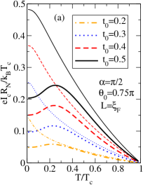
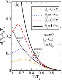
Figure 7: (Color online) Critical Josephson current $I_{\rm c}$ multiplied with the normal state resistance $R_{\rm N}$ for an S/HM/S Josephson junction with magnetic interfaces (thick lines) and for an S/N/S junction with non-magnetic interfaces (thin lines). In (a) for both cases, the transmission amplitudes $t_{0}$ are varied from 0.2 to 0.5. The spin-mixing angle for normal impact is $\vartheta_{0}=0.75\pi$, and the junction length $L$ is equal to the coherence length in the half metal, $\xi_{\rm F}=v_{\rm F}/2\pi T_{\rm c}$. In (b) we fix $L=3\xi_{\rm F}$, $t_{0}=0.5$, and vary for the S/HM/S junction the spin mixing angle. For (a) and (b) the interface spin misalignment angle is $\alpha=\pi/2$.

In Fig. 7(a) we show results obtained with Eq. 200. Shown is the critical Josephson current multiplied with the normal state resistance obtained by Eq. 201. For definiteness we present results for identical isotropic Fermi surfaces on both sides of the interface and for the dependence of the transmission amplitude $t$ on the impact angle $\theta_{p}$ (measured from the surface normal) appropriate for a $\delta$-potential, $t(\theta_{p})=t_{0}\cos\theta_{p}/\sqrt{1-t_{0}^{2}\sin^{2}\theta_{p}}$, where $t_{0}$ is the transmission for normal impact. For the spin mixing angle $\vartheta$ we assume a dependence $\vartheta=\vartheta_{0}\cos(\theta_{p})$. For comparison we also show the corresponding values for a superconductor/normal-metal/superconductor (S/N/S) Josephson junction. As can be seen, the supercurrent through a half metal can be of a similar magnitude as through a normal metal, provided the parameter $P$ is of order one.

In fact, as can be seen in Fig. 7(b), the $I_{\rm c}R_{\rm N}$-product can exceed that for an analogous S/N/S junction. The reason for this enhancement are current carrying Andreev bound states below the gap energy, that are discussed further below. We show for several values of $\vartheta_{0}$ the $I_{\rm c}R_{\rm N}$-product in comparison with that for a non-magnetic S/N/S Josephson junction with the same transmission probability and same length. With increasing $\vartheta_{0}$ the magnitude of the effect increases, and the maximum in the temperature dependence moves to lower temperatures.

In fact, for the special case that $P=1$ (i.e. $t=1$, $\vartheta=\pi$, $\alpha=\pi/2$) for all Fermi surface points, the maximum becomes unobservable because it moves to zero temperature, as has been noted also in Ref. galak08, . In this case, furthermore, we have $\beta=\zeta=(1-\gamma_{\rm S}\tilde{\gamma}_{\rm S})$, $\eta=-\gamma_{\rm S}\tilde{\gamma}_{\rm S}(1-\gamma_{\rm S}\tilde{\gamma}_{\rm S})$ for the S/HM/S junction, and $\beta=i$, $\zeta=1$, $\eta=\gamma_{\rm S}\tilde{\gamma}_{\rm S}$ for the S/N/S junction. Consequently, after canceling the common factor $(1-\gamma_{\rm S}\tilde{\gamma}_{\rm S})$ in Eq. 199 for the S/HM/S junction, it is seen that $1/p_{\pm}$ at phase $\chi$ for the S/HM/S junction coincides with $1/p_{\pm}$ at phase $(\chi+\pi)$ for the S/N/S junction. This proves that the $I_{\rm c}R_{\rm N}$-product for $P=1$ is equal to that for the corresponding S/N/S junction, and the corresponding current phase relations are shifted by $\pi$. This result is in agreement with the findings in section III.D of Ref. galak08, for the short and long junction limits, that were obtained within the more general Gor’kov formalism.

We caution however, that the suppression of the singlet order parameter at the interface cannot be neglected for $P$ close to $1$, unless a strong Fermi surface mismatch is present (in which case the transmission is reduced due to the Fermi velocity mismatch), and self-consistent calculations must be performed as done in Ref. eschrig03, .

V.2.3 Local density of states

We now proceed to calculate the local density of states as function of energy. For this we need to perform an analytical continuation to the real energy axis. We define in this case $y=e^{izL/\mu v_{\rm F}}$ and $\gamma_{\rm S}=-\tilde{\gamma}_{\rm S}=-|{\it\Delta}|/(z+i\sqrt{|{\it\Delta}|^{2}-z^{2}})$ with $z=\epsilon+i0^{+}$. The momentum resolved density of states is then given in the center of the half metal by,

$$\frac{N_{\pm}}{N_{\rm F}} = -\;\frac{1}{\pi}\mbox{Im}g^{\scriptscriptstyle\rm R}_{\pm}=\mbox{Re}\frac{1+\tilde{\gamma}_{\pm}\gamma_{\pm}}{1-\tilde{\gamma}_{\pm}\gamma_{\pm}}$$ (204)

$$= \mbox{Re}\left[\left(1-\frac{4}{p_{\pm}(\epsilon)^{2}}\right)^{-\frac{1}{2}}\right].$$

The local density of states is obtained as

$$N(\epsilon)=\langle N_{+}+N_{-}\rangle_{\rm FS_{+}}.$$ (205)

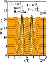
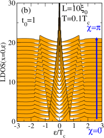
Figure 8: (Color online) Local density of states in the center of a current biased high-transmissive symmetric Josephson junction for (a) an S/HM/S junction and (b) an S/N/S junction. In both cases the phase difference over the junction is varied from 0 to $\pi$. The remaining parameters are indicated.

In Fig. 8 we compare the local density of states (LDOS) for an S/HM/S-junction and an S/N/S-junction in the high-transmission limit for a symmetric setup. For clarity of presentation we have vertically shifted the curves with respect to each other. The junctions are current biased, and the phase difference varies in both cases from 0 to $\pi$ as indicated. For the S/N/S-junction the well-known Andreev-Saint-James statesandreev64 ; saint64 are seen (for a review see Ref. deutscher05, ) with a reduction of the LDOS at low bias except for the case of $\chi=\pi$, when a zero bias bound state is present. In contrast, for the S/HM/S-junction there is a low-energy band of bound states. This behavior has already been noted in Ref. eschrig03, . Note that $\chi=\pi$ is the equilibrium phase of the S/HM/S junction.eschrig03 The dispersion of the Andreev peaks in the spectra with $\chi$ indicates the direction of the current that is carried by them. For the S/N/S-junction the lowest bias peak dominates, that carries current in positive direction, whereas for the S/HM/S-junction the low-energy band is responsible for the low-temperature anomaly $J_{\rm c}(T)$, and the next higher band carries most of the current, that is in negative direction, in accordance with the $\pi$-junction behavior.

The half-width $W_{1/2}$ of the low-energy band varies with the interface parameters, with the impact angle, with the phase difference $\chi$, with temperature, and with junction length. In general the width of the low-energy band is larger for $\chi=0$ than for $\chi=\pi$.

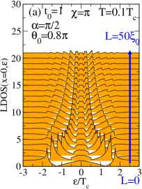
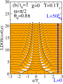
Figure 9: (Color online) Local density of states in the center of a current biased high-transmissive symmetric S/HM/S Josephson junction, for (a) a phase difference over the junction of $\pi$ and (b) of $0$. In both cases the junction length is varied from the short junction limit to $L=50\xi_{\rm F}$. The remaining parameters are indicated.

In Fig. 9, we show its dependence on the junction length for (a) a $\pi$-junction and (b) a zero-junction. In the short-junction limit the half-width for $t=1$ is given by $W_{1/2}(\chi=\pi)=|{\it\Delta}|(\sqrt{2-P^{2}}-P)/2$ and $W_{1/2}(\chi=0)=|{\it\Delta}|\sqrt{1-P^{2}}$. In the limit of small $P$ (but still $t=1$) we obtain $W_{1/2}(\chi=\pi)\to|{\it\Delta}|/\sqrt{2}$ and $W_{1/2}(\chi=0)\to|{\it\Delta}|$. For the special case $P=1$ the spectra are equal to those for an S/N/S-junction with the junction phase shifted by $\pi$ (see the corresponding discussion in the last subsection), i.e. the low energy band vanishes in the limit $P\to 1$ for a $\pi$ junction and a zero energy bound state appears for a zero-junction. In general, as $P$ varies with $\vartheta$ and thus with the impact angle, the width of the low-energy band in Figs. 8(a) and 9 is a superposition for many different $P$. The overall width of the low-energy band is set by the values for smallest $P$, the kink-features closer to the chemical potential correspond to the largest $P$ for trajectories with normal impact.

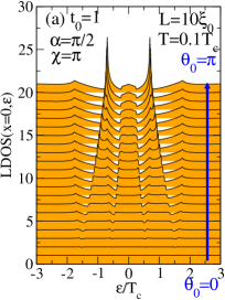
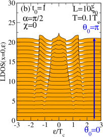
Figure 10: (Color online) Local density of states in the center of a current biased high-transmissive symmetric S/HM/S Josephson junction, for (a) a phase difference over the junction of $\pi$ and (b) of $0$. In both cases the spin mixing angle $\vartheta_{0}$ is varied from 0 to $\pi$. The remaining parameters are indicated.

In Fig. 10 we show results for the variation of the LDOS with with the spin-mixing angle $\vartheta_{0}$ for (a) a $\pi$-junction and (b) a zero-junction. For the zero-junction a peak appears at high $\vartheta_{0}$, that is a signature of the zero bias bound state for normal impact when $P=1$. For smaller spin-mixing angles in general the structures get smeared out, and a set of energy bands separated by narrower suppressions of the LDOS remains.

V.3 Point contact geometry

V.3.1 Distribution functions

For the distribution functions, we introduce the notation,

$$\hat{\mbox{\boldmath$x$}}^{\prime}=\left(\begin{array}[]{cc}\hat{x}^{\prime}_{\rm S}&\mid\!{x}\rangle^{\prime}\\ \langle{x}\!\mid^{\prime}&x^{\prime}_{\rm F}\end{array}\right)={\mbox{\boldmath$S$}}^{\scriptscriptstyle\rm R}\left(\begin{array}[]{cc}\hat{x}_{\rm S}&0\\ 0&x_{\rm F}\end{array}\right){\mbox{\boldmath$S$}}^{\scriptscriptstyle\rm A}$$ (210)

with ${\mbox{\boldmath$S$}}^{\scriptscriptstyle\rm A}=({\mbox{\boldmath$S$}}^{\scriptscriptstyle\rm R})^{\dagger}$, which explicitely gives

$$\hat{x}^{\prime}_{\rm S} = \hat{R}_{\rm S}^{\scriptscriptstyle\rm R}\;\hat{x}_{\rm S}\hat{R}_{\rm S}^{\scriptscriptstyle\rm A}+x_{\rm F}\mid\!{T}\rangle^{\scriptscriptstyle\rm R}\langle{T}\!\mid^{\scriptscriptstyle\rm A}$$ (211)

$$\mid\!{x}\rangle^{\prime} = \hat{R}_{\rm S}^{\scriptscriptstyle\rm R}\;\hat{x}_{\rm S}\mid\!{T}\rangle^{\scriptscriptstyle\rm A}-x_{\rm F}\;R_{\rm F}^{\scriptscriptstyle\rm A}\;\mid\!{T}\rangle^{\scriptscriptstyle\rm R}$$ (212)

$$\langle{x}\!\mid^{\prime} = \langle{T}\!\mid^{\scriptscriptstyle\rm R}\hat{x}_{\rm S}\;\hat{R}_{\rm S}^{\scriptscriptstyle\rm A}-x_{\rm F}\;R_{\rm F}^{\scriptscriptstyle\rm R}\;\langle{T}\!\mid^{\scriptscriptstyle\rm A}$$ (213)

$$x^{\prime}_{\rm F} = \langle{T}\!\mid^{\scriptscriptstyle\rm R}\hat{x}_{\rm S}\mid\!{T}\rangle^{\scriptscriptstyle\rm A}+x_{\rm F}\;R_{\rm F}^{\scriptscriptstyle\rm R}\;R_{\rm F}^{\scriptscriptstyle\rm A}.$$ (214)

with $\hat{R}_{\rm S}^{\scriptscriptstyle\rm A}=(\hat{R}_{\rm S}^{\scriptscriptstyle\rm R})^{\dagger}$, $\mid\!{T}\rangle^{\scriptscriptstyle\rm A}=(\langle{T}\!\mid^{\scriptscriptstyle\rm R})^{\dagger}$, $\langle{T}\!\mid^{\scriptscriptstyle\rm A}=(\mid\!{T}\rangle^{\scriptscriptstyle\rm R})^{\dagger}$, $R_{\rm F}^{\scriptscriptstyle\rm A}=(R_{\rm F}^{\scriptscriptstyle\rm R})^{\ast}$. Then, with the abbreviations

$$\mid\!{{\it\Gamma}}\rangle^{\scriptscriptstyle\rm R} = \mid\!{\gamma}\rangle^{\prime}(1-\tilde{\gamma}_{\rm F}\gamma^{\prime}_{\rm F})^{-1}$$ (215)

$$\langle{{\it\Gamma}}\!\mid^{\scriptscriptstyle\rm R} = \langle{\gamma}\!\mid^{\prime}\left(\hat{1}-\hat{\tilde{\gamma}}_{\rm S}\hat{\gamma}^{\prime}_{\rm S}\right)^{-1},$$ (216)

and $\mid\!{{\it\Gamma}}\rangle^{\scriptscriptstyle\rm A}=(\langle{{\,\tilde{\!{\it\Gamma}}}}\!\mid^{\scriptscriptstyle\rm R})^{\dagger}$, $\langle{{\it\Gamma}}\!\mid^{\scriptscriptstyle\rm A}=(\mid\!{{\,\tilde{\!{\it\Gamma}}}}\rangle^{\scriptscriptstyle\rm R})^{\dagger}$, the explicit boundary conditions, Eq. (112), for the distribution functions read,

$$\hat{X}_{\rm S} = \hat{x}^{\prime}_{\rm S}+\gamma_{\rm F}^{\scriptscriptstyle\rm A}\mid\!{x}\rangle^{\prime}\langle{{\,\tilde{\!{\it\Gamma}}}}\!\mid^{\scriptscriptstyle\rm A}+\tilde{\gamma}_{\rm F}^{\scriptscriptstyle\rm R}\mid\!{{\it\Gamma}}\rangle^{\scriptscriptstyle\rm R}\langle{x}\!\mid^{\prime}$$ (217)

$$\qquad+(\tilde{\gamma}^{\scriptscriptstyle\rm R}_{\rm F}x^{\prime}_{\rm F}\gamma_{\rm F}^{\scriptscriptstyle\rm A}-\tilde{x}_{\rm F})\mid\!{{\it\Gamma}}\rangle^{\scriptscriptstyle\rm R}\langle{{\,\tilde{\!{\it\Gamma}}}}\!\mid^{\scriptscriptstyle\rm A}$$

$$X_{\rm F} = x^{\prime}_{\rm F}+\langle{x}\!\mid^{\prime}\;\hat{\gamma}_{\rm S}^{\scriptscriptstyle\rm A}\;\mid\!{{\,\tilde{\!{\it\Gamma}}}}\rangle^{\scriptscriptstyle\rm A}+\langle{{\it\Gamma}}\!\mid^{\scriptscriptstyle\rm R}\;\hat{\tilde{\gamma}}_{\rm S}^{\scriptscriptstyle\rm R}\;\mid\!{x}\rangle^{\prime}$$ (218)

$$\qquad+\langle{{\it\Gamma}}\!\mid^{\scriptscriptstyle\rm R}\;(\hat{\tilde{\gamma}}^{\scriptscriptstyle\rm R}_{\rm S}\hat{x}^{\prime}_{\rm S}\hat{\gamma}_{\rm S}^{\scriptscriptstyle\rm A}-\hat{\tilde{x}}_{\rm S})\;\mid\!{{\,\tilde{\!{\it\Gamma}}}}\rangle^{\scriptscriptstyle\rm A}$$

Here, $\hat{\gamma}_{\rm S}^{\scriptscriptstyle\rm A}=(\hat{\tilde{\gamma}}_{\rm S}^{\scriptscriptstyle\rm R})^{\dagger}$, $\gamma_{\rm F}^{\scriptscriptstyle\rm A}=(\tilde{\gamma}_{\rm F}^{\scriptscriptstyle\rm R})^{\ast}$.

V.3.2 Point contact spectra

Superconductor/half-metal point contact spectra have been studied experimentally in a number of cases.soulen98 ; desisto00 ; ji01 ; angu01 ; parker02 ; woods04 ; dyachenko06 ; yates07 ; krivoruchko08 ; bocklage07 However, the analysis in all these studies did not include the effect of spin active interface scattering. Here, we show how such effects can be taken into account in a ballistic point contact. We assume incoming solutions to be in equilibrium. The treatment in terms of coherence and distribution functions can be simplified considerably by using the symmetries described in Appendix F.2. Proceeding along the lines described there, we introduce anomalous distribution functions by $\hat{g}^{K}[x,\tilde{x}]-\hat{g}^{K}[x_{0},\tilde{x}_{0}]=\hat{g}^{\scriptscriptstyle\rm R}\hat{F}_{0}-\hat{F}_{0}\hat{g}^{\scriptscriptstyle\rm A}$, with

$$\hat{F}_{0}=\left(\begin{array}[]{cc}F_{0}&0\\ 0&-\tilde{F}_{0}\end{array}\right)$$ (221)

and $x_{0}=x-(F_{0}+\gamma^{\scriptscriptstyle\rm R}\tilde{F}_{0}\tilde{\gamma}^{\scriptscriptstyle\rm A})$. We use for $F_{0}$ the equilibrium distribution function in the superconductor. Then, the incoming anomalous distribution functions $x_{S,0}$ and $\tilde{x}_{S,0}$ in the superconductor are zero. For the half metal we have $x_{\rm F}=F+\gamma^{\scriptscriptstyle\rm R}_{\rm F}\tilde{F}\tilde{\gamma}^{\scriptscriptstyle\rm A}_{\rm F}$ with $F=\tanh[(\epsilon-eV)/2T]$ and $\tilde{F}=-\tanh[(\epsilon+eV)/2T]$, and consequently $x_{F,0}=(F-F_{0})+\gamma^{\scriptscriptstyle\rm R}_{\rm F}(\tilde{F}-\tilde{F}_{0})\tilde{\gamma}^{\scriptscriptstyle\rm A}_{\rm F}$. Furthermore, for a ballistic point contact the incoming coherence functions on the half-metallic side are zero, $\gamma_{\rm F}=\tilde{\gamma}_{\rm F}=0$. From here on we drop the index “0” for all distribution functions in order to not overload the notation, and keep in mind that they are all anomalous.

Substituting all this into Eq. (218), one arrives at

$$X_{\rm F}-x_{\rm F}=-\frac{x_{\rm F}t^{2}}{|\zeta^{\scriptscriptstyle\rm R}|^{2}}\Big{\{}(1-{\it\Pi}_{2})\left[1+r^{2}{\it\Pi}_{2}-r\cos(\vartheta){\it\Sigma}_{2}\right.\Big{.}$$

$$\qquad\quad+\Big{.}\left.r\cos(\alpha)\sin(\vartheta){\it\Delta}_{2}\right]\Big{.}$$

$$\qquad\quad+\Big{.}t^{2}P^{2}(1+r)\left[{\it\Sigma}_{2}(1+r{\it\Pi}_{2})+2(1+r){\it\Pi}_{2}\right]\Big{\}}$$

$$-{\it\Gamma}_{\rm F}^{\scriptscriptstyle\rm R}\tilde{x}_{\rm F}{\,\tilde{\!{\it\Gamma}}}_{\rm F}^{\scriptscriptstyle\rm A}=-\frac{\tilde{x}_{\rm F}t^{4}}{|\zeta^{\scriptscriptstyle\rm R}|^{2}}P^{2}(1+r)^{2}|\gamma_{\rm S}^{\scriptscriptstyle\rm R}|^{2}\left[1+{\it\Sigma}_{2}+{\it\Pi}_{2}\right]$$

with

$${\it\Pi}_{2} = (\gamma_{\rm S}^{\scriptscriptstyle\rm R}\tilde{\gamma}_{\rm S}^{\scriptscriptstyle\rm R})(\gamma_{\rm S}^{\scriptscriptstyle\rm A}\tilde{\gamma}_{\rm S}^{\scriptscriptstyle\rm A})^{2}=|\gamma_{\rm S}^{\scriptscriptstyle\rm R}\tilde{\gamma}_{\rm S}^{\scriptscriptstyle\rm R}|^{2}$$ (223)

$${\it\Sigma}_{2} = -(\gamma_{\rm S}^{\scriptscriptstyle\rm R}\tilde{\gamma}_{\rm S}^{\scriptscriptstyle\rm R}+\gamma_{\rm S}^{\scriptscriptstyle\rm A}\tilde{\gamma}_{\rm S}^{\scriptscriptstyle\rm A})=-2\mbox{Re}(\gamma_{\rm S}^{\scriptscriptstyle\rm R}\tilde{\gamma}_{\rm S}^{\scriptscriptstyle\rm R})$$ (224)

$${\it\Delta}_{2} = -\frac{1}{i}(\gamma_{\rm S}^{\scriptscriptstyle\rm R}\tilde{\gamma}_{\rm S}^{\scriptscriptstyle\rm R}-\gamma_{\rm S}^{\scriptscriptstyle\rm A}\tilde{\gamma}_{\rm S}^{\scriptscriptstyle\rm A})=-2\mbox{Im}(\gamma_{\rm S}^{\scriptscriptstyle\rm R}\tilde{\gamma}_{\rm S}^{\scriptscriptstyle\rm R}),$$ (225)

and we have used the notation $\hat{\gamma}_{\rm S}^{\scriptscriptstyle\rm R}=\gamma_{\rm S}^{\scriptscriptstyle\rm R}i\sigma_{y}$ and $\hat{\gamma}_{\rm S}^{\scriptscriptstyle\rm A}=\gamma_{\rm S}^{\scriptscriptstyle\rm A}i\sigma_{y}$, meaning that $\tilde{\gamma}_{\rm S}^{\scriptscriptstyle\rm A}=-(\gamma_{\rm S}^{\scriptscriptstyle\rm R})^{\ast}$. These expressions are still general and we only made use of zero incoming $\gamma_{\rm F}$, $\tilde{\gamma}_{\rm F}$, $x_{S,0}$, and $\tilde{x}_{S,0}$.

The current density from the half metal to the superconductor is given in terms of the anomalous distribution functions by,

$$j=eN_{\rm F}v_{\rm F}\int\frac{d\epsilon}{2}\;\Big{\langle}\mu(X_{\rm F}-x_{\rm F}-{\it\Gamma}_{\rm F}^{\scriptscriptstyle\rm R}\tilde{x}_{\rm F}{\,\tilde{\!{\it\Gamma}}}_{\rm F}^{\scriptscriptstyle\rm A})\Big{\rangle}_{\rm FS_{+}}$$ (226)

with $x_{\rm F}=F-F_{0}=[\tanh\frac{\epsilon-eV}{2T}-\tanh\frac{\epsilon}{2T}]$, and $\tilde{x}_{\rm F}=\tilde{F}-\tilde{F}_{0}=-[\tanh\frac{\epsilon+eV}{2T}-\tanh\frac{\epsilon}{2T}]$. The current density can be written as

$$j = eN_{\rm F}v_{\rm F}\int_{-\infty}^{\infty}\frac{d\epsilon}{4}\;j_{\epsilon}\left(\tanh\frac{\epsilon+eV}{2T}-\tanh\frac{\epsilon-eV}{2T}\right)$$

with spectral current kernels $j_{\epsilon}$. The normal state boundary resistance is $1/R_{\rm N}A=j_{\rm N}/V=e^{2}N_{\rm F}v_{\rm F}\langle\mu t^{2}\rangle_{\rm FS_{+}}$.

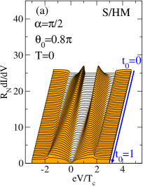
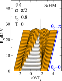
Figure 11: (Color online) Point contact spectra for an S/HM contact. In (a) the transmission $t_{0}$ varied from 0 to 1, and in (b) the spin-mixing angle $\vartheta_{0}$ is varied from 0 to $\pi$. Both quantities depend on the quasiparticle impact angle as discussed in the text. The remaining parameters are indicated.

Further simplifications arise for incoming homogeneous distribution functions, when $\tilde{\gamma}_{\rm S}^{\scriptscriptstyle\rm R}=-\gamma_{\rm S}^{\scriptscriptstyle\rm R}$. Then, noting that for $|\epsilon|<|{\it\Delta}|$ we have ${\it\Pi}_{2}=1$, it follows that

$$X_{\rm F}-x_{\rm F} = -\frac{x_{\rm F}t^{4}}{|\zeta^{\scriptscriptstyle\rm R}|^{2}}P^{2}(1+r)^{2}({\it\Sigma}_{2}+2)$$ (228)

$$-\Gamma_{\rm F}^{\scriptscriptstyle\rm R}\tilde{x}_{\rm F}\tilde{\Gamma}_{\rm F}^{\scriptscriptstyle\rm A} = -\frac{\tilde{x}_{\rm F}t^{4}}{|\zeta^{\scriptscriptstyle\rm R}|^{2}}P^{2}(1+r)^{2}({\it\Sigma}_{2}+2)$$ (229)

leading to the Andreev spectral current

$$j_{\epsilon}=\left\langle\frac{\mu\cdot 4P^{2}t^{4}(1+r)^{2}\cdot\big{(}1+\mbox{Re}[(\gamma_{\rm S}^{\scriptscriptstyle\rm R})^{2}]\big{)}}{\Big{|}1+(\gamma_{\rm S}^{\scriptscriptstyle\rm R})^{4}r^{2}-2(\gamma_{\rm S}^{\scriptscriptstyle\rm R})^{2}r\cos(\vartheta)+(\gamma_{\rm S}^{\scriptscriptstyle\rm R})^{2}P^{2}t^{4}\Big{|}^{2}}\right\rangle_{\!\!\!\!\rm FS_{+}}\!\!\!\!\!\!.$$ (230)

For zero misalignment of the interface moments, $\alpha=0$ leads to $P=0$, and there is no Andreev current. For $|\epsilon|>|{\it\Delta}|$, additional terms become important, associated with ${\it\Pi}_{2}\neq 1$. Here, because $\gamma_{\rm S}^{\scriptscriptstyle\rm R}$ is real, and thus $\tilde{x}_{\rm F}(\epsilon)=-x_{\rm F}(-\epsilon)$, we obtain

$$j_{\epsilon}=\left\langle\frac{\mu t^{2}\cdot[1-(\gamma_{\rm S}^{\scriptscriptstyle\rm R})^{4}]}{1+(\gamma_{\rm S}^{\scriptscriptstyle\rm R})^{4}r^{2}-2(\gamma_{\rm S}^{\scriptscriptstyle\rm R})^{2}r\cos(\vartheta)+(\gamma_{\rm S}^{\scriptscriptstyle\rm R})^{2}P^{2}t^{4}}\right\rangle_{\rm FS_{+}}$$

$$+\left\langle\frac{\mu\cdot 2P^{2}t^{4}(1+r)^{2}\cdot[1+(\gamma_{\rm S}^{\scriptscriptstyle\rm R})^{2}]^{2}(\gamma_{\rm S}^{\scriptscriptstyle\rm R})^{2}}{\Big{|}1+(\gamma_{\rm S}^{\scriptscriptstyle\rm R})^{4}r^{2}-2(\gamma_{\rm S}^{\scriptscriptstyle\rm R})^{2}r\cos(\vartheta)+(\gamma_{\rm S}^{\scriptscriptstyle\rm R})^{2}P^{2}t^{4}\Big{|}^{2}}\right\rangle_{\!\!\!\!\rm FS_{+}}\!\!\!\!\!\!.$$

For comparison, we also present the expressions for the corresponding ${\rm d}I/{\rm d}V$-spectra for a normal metal, $j_{\epsilon}=1+\left\langle\mu[t^{4}|\gamma_{\rm S}^{\scriptscriptstyle\rm R}|^{2}-r^{2}|1-(\gamma_{\rm S}^{\scriptscriptstyle\rm R})^{2}|^{2}]/|1-r^{2}(\gamma_{\rm S}^{\scriptscriptstyle\rm R})^{2}|^{2}\right\rangle_{\rm FS_{+}}$. This gives $j_{\epsilon}=\left\langle 2\mu t^{4}/|1-r^{2}(\gamma_{\rm S}^{\scriptscriptstyle\rm R})^{2}|^{2}\right\rangle_{\rm FS_{+}}$, for $|\epsilon|<|{\it\Delta}|$, and $j_{\epsilon}=\left\langle\mu t^{2}[1+(\gamma_{\rm S}^{\scriptscriptstyle\rm R})^{2}]/[1-r^{2}(\gamma_{\rm S}^{\scriptscriptstyle\rm R})^{2}]\right\rangle_{\rm FS_{+}}$ for $|\epsilon|>|{\it\Delta}|$.

In Fig. 11 we show representative results for zero temperature S/HM point-contact spectra for various transmissions and spin-mixing angles. In general, there are sub-gap states present in the spectra except for very small $\vartheta_{0}$, $\alpha$, or $t_{0}$. For the special case $\vartheta_{0}=\pi$ there is a sharp zero bias state observable in the spectra. Otherwise, if $\vartheta_{0}$ is not close to $\pi$, ${\rm d}I/{\rm d}V$ is for $T=0$ zero at zero bias and increases quadratic with the voltage. The details of the spectra will depend on the Fermi surface mismatch and the interface characteristics, in particular the dependence of the various parameters on impact angle. We leave a detailed discussion of these issues for a future publication.

VI Acknowledgments

I would like to thank for valuable discussions with Jaime Ferrer, Mikael Fogelström, Tomas Löfwander, Jim Sauls, Anton Vorontsov, Sungkit Yip, and Erhai Zhao about quasiclassical boundary conditions, and with Roland Grein, Juha Kopu, Tomas Löfwander, Georgo Metalidis, and Gerd Schön about superconductor/half-metal heterostructures. I also acknowledge the hospitality of the Aspen Center for Physics, where part of this work was done.

Appendix A Time convolution product

We use extensively the non-commutative ${\circ}$-product between two functions, which allows us to formulate the equations independently from the representation of the dynamical coordinates (time, energy, mixed). In the time domain, the non-commutative ${\circ}$-product between two functions $\hat{A}(t,t^{\prime})$ and $\hat{B}(t,t^{\prime})$ is defined by

$$\hat{A}{\circ}\hat{B}(t,t^{\prime})=\int{\rm d}t^{\prime\prime}\;\hat{A}(t,t^{\prime\prime})\hat{B}(t^{\prime\prime},t^{\prime}),$$ (232)

with the unit element $\hat{\it 1}=\delta(t-t^{\prime})\hat{1}$. In an energy representation (after a Fourier transform $t\to\epsilon$, $t^{\prime}\to\epsilon^{\prime}$), the product reads

$$\hat{A}{\circ}\hat{B}(\epsilon,\epsilon^{\prime})=\int\frac{{\rm d}\epsilon^{\prime\prime}}{2\pi}\;\hat{A}(\epsilon,\epsilon^{\prime\prime})\hat{B}(\epsilon^{\prime\prime},\epsilon^{\prime}),$$ (233)

with the unit element $\hat{\it 1}=\delta(\epsilon-\epsilon^{\prime})\hat{1}$. In a mixed representation, when performing a Fourier transform $(t-t^{\prime})\to\epsilon$, and keeping the time variable $(t+t^{\prime})/2\to t$, the product can be written as

$$\hat{A}{\circ}\hat{B}(\epsilon,t)=\mbox{e}^{\frac{i\hbar}{2}(\partial_{\epsilon}^{\scriptscriptstyle\rm A}\partial_{t}^{B}-\partial_{t}^{\scriptscriptstyle\rm A}\partial_{\epsilon}^{B})}\hat{A}(\epsilon,t)\hat{B}(\epsilon,t)\quad,$$ (234)

and the unit element is $\hat{\it 1}=\hat{1}$. If one of the factors is both independent of $\epsilon$ and $t$, the ${\circ}$-product reduces to the usual matrix product. Note that in a mixed representation

$$\epsilon{\circ}a-a{\circ}\epsilon=i\hbar\partial_{t}a,\qquad\epsilon{\circ}a+a{\circ}\epsilon=2\epsilon a.$$ (235)

Sometimes (for example when performing a perturbation theory out of the equilibrium) a modified energy representation is useful, where one performs Fourier transforms $(t-t^{\prime})\to\epsilon$, $(t+t^{\prime})/2\to\omega$. In this case the product reads

$$\hat{A}{\circ}\hat{B}(\epsilon,\omega) = \int\limits_{-\infty}^{\infty}\frac{\mbox{d}\omega^{\prime}}{2\pi}\frac{\mbox{d}\omega^{\prime\prime}}{2\pi}\delta(\omega^{\prime}+\omega^{\prime\prime}-\omega)\times$$ (236)

$$\times\hat{A}(\mbox{$\epsilon\!+\!{\hbar\omega^{\prime}\over 2}$},\omega^{\prime\prime})\hat{B}(\mbox{$\epsilon\!-\!{\hbar\omega^{\prime\prime}\over 2}$},\omega^{\prime})\quad,$$

and the unit element is $\hat{\it 1}=\delta(\omega)\hat{1}$. If $\hat{A}(\epsilon,t)=\hat{A}(\epsilon)$ is independent of $t$ (if $\hat{A}$ is an equilibrium quantity) then

$$\hat{A}{\circ}\hat{B}(\epsilon,\omega)=\hat{A}(\mbox{$\epsilon\!+\!{\hbar\omega\over 2}$})\hat{B}(\epsilon,\omega)\quad,$$ (237)

and, analogously, if $\hat{B}$ is an equilibrium quantity

$$\hat{A}{\circ}\hat{B}(\epsilon,\omega)=\hat{A}(\epsilon,\omega)\hat{B}(\mbox{$\epsilon\!-\!{\hbar\omega\over 2}$})\quad.$$ (238)

We also generalize throughout the paper the commutator

$$[\hat{A},\hat{B}]_{{\circ}}=\hat{A}{\circ}\hat{B}-\hat{B}{\circ}\hat{A}\;.$$ (239)

A useful identity is

$$\left(1+a{\circ}b\right)^{-1}{\circ}a=a{\circ}\left(1+b{\circ}a\right)^{-1}.$$ (240)

Appendix B Projectors

We adopt here the notation of Ref. eschrig00, , Appendix B. Following Shelankov,shelankov85 we introduce the following projectors

$$\check{P}_{\pm}=\frac{1}{2}\left(\check{1}\pm\frac{\;1}{-i\pi}\;\check{g}\right)$$ (241)

with the properties $\check{P}_{+}{\circ}\check{P}_{+}=\check{P}_{+}$ , $\check{P}_{-}{\circ}\check{P}_{-}=\check{P}_{-}$, $\check{P}_{+}+\check{P}_{-}=\check{1}$, and $\check{P}_{+}{\circ}\check{P}_{-}=\check{P}_{-}{\circ}\check{P}_{+}=\check{0}$. The quasiclassical Green’s function is expressed in terms of $\check{P}_{+}$ or $\check{P}_{-}$ by,

$$\check{g} = -i\pi\left(\check{P}_{+}-\check{P}_{-}\right)\,.$$ (242)

From the normalization condition, the Keldysh component of the Green’s function, $\hat{g}^{{\scriptscriptstyle\rm K}}$, fulfills the relations $\hat{P}_{+}^{{\scriptscriptstyle\rm R}}{\circ}\hat{g}^{{\scriptscriptstyle\rm K}}{\circ}\hat{P}_{+}^{{\scriptscriptstyle\rm A}}=\hat{0}$ and $\hat{P}_{-}^{{\scriptscriptstyle\rm R}}{\circ}\hat{g}^{{\scriptscriptstyle\rm K}}{\circ}\hat{P}_{-}^{{\scriptscriptstyle\rm A}}=\hat{0}$, which allows a parameterization by

$$\hat{g}^{{\scriptscriptstyle\rm K}}=-2\pi\;i\;\left[\hat{P}_{+}^{{\scriptscriptstyle\rm R}}{\circ}\hat{X}^{{\scriptscriptstyle\rm K}}{\circ}\hat{P}_{-}^{{\scriptscriptstyle\rm A}}+\hat{P}_{-}^{{\scriptscriptstyle\rm R}}{\circ}\hat{Y}^{{\scriptscriptstyle\rm K}}{\circ}\hat{P}_{+}^{{\scriptscriptstyle\rm A}}\right]\;,$$ (243)

were $\hat{X}^{{\scriptscriptstyle\rm K}}$ and $\hat{Y}^{{\scriptscriptstyle\rm K}}$ are related by symmetry relations. The function $\hat{X}^{{\scriptscriptstyle\rm K}}$ can be chosen in a convenient way.

Analogously, for the linear response to an external perturbation, the normalization condition leads to $\hat{P}_{+}^{{\scriptscriptstyle\rm R,A}}{\circ}{\delta}\!\hat{g}^{{\scriptscriptstyle\rm R,A}}{\circ}\hat{P}_{+}^{{\scriptscriptstyle\rm R,A}}=\hat{0}$ and $\hat{P}_{-}^{{\scriptscriptstyle\rm R,A}}{\circ}{\delta}\!\hat{g}^{{\scriptscriptstyle\rm R,A}}{\circ}\hat{P}_{-}^{{\scriptscriptstyle\rm R,A}}=\hat{0}$; as a consequence the spectral response, ${\delta}\!\hat{g}^{{\scriptscriptstyle\rm R,A}}$, can be written as

$${\delta}\!\hat{g}^{{\scriptscriptstyle\rm R,A}}=\mp 2\pi i\left[\hat{P}_{+}{\circ}{\delta}\!\hat{W}{\circ}\hat{P}_{-}-\hat{P}_{-}{\circ}{\delta}\!\hat{Z}{\circ}\hat{P}_{+}\right]^{{\scriptscriptstyle\rm R,A}}$$ (244)

with a suitable parameterization of the functions ${\delta}\!\hat{W}$ and ${\delta}\!\hat{Z}$.

Appendix C Parameter representations of Projectors

The projectors $\hat{P}_{+}^{{\scriptscriptstyle\rm R}}$ and $\hat{P}_{-}^{{\scriptscriptstyle\rm R}}$ may be parameterized by complex spin matrices $\gamma^{{\scriptscriptstyle\rm R}}$ and $\tilde{\gamma}^{{\scriptscriptstyle\rm R}}$ as defined in Appendix C of Ref. eschrig00, . Alternatively, we give here the parameterization in terms of ${\cal G}$, ${\cal F}$, $\tilde{\cal G}$, and $\tilde{\cal F}$. We obtain

$$\hat{P}_{+}^{{\scriptscriptstyle\rm R}}=\left(\begin{array}[]{cc}\;\;\,{\cal G}&{\cal F}\\ -\tilde{\cal F}&(1-\tilde{\cal G})\end{array}\right)^{{\scriptscriptstyle\rm R}},\hat{P}_{-}^{{\scriptscriptstyle\rm R}}=\left(\begin{array}[]{cc}(1-{\cal G})&-{\cal F}\\ \tilde{\cal F}&\tilde{\cal G}\end{array}\right)^{{\scriptscriptstyle\rm R}}.$$ (249)

$$\hat{P}_{+}^{{\scriptscriptstyle\rm A}}=\left(\begin{array}[]{cc}(1-\tilde{\cal G})&-{\cal F}\\ \tilde{\cal F}&\tilde{\cal G}\end{array}\right)^{{\scriptscriptstyle\rm A}},\hat{P}_{-}^{{\scriptscriptstyle\rm A}}=\left(\begin{array}[]{cc}\;\;\,{\cal G}&{\cal F}\\ -\tilde{\cal F}&(1-\tilde{\cal G})\end{array}\right)^{{\scriptscriptstyle\rm A}}.$$ (254)

Appendix D Parameter representations of distribution functions

In general the functions $\hat{X}^{{\scriptscriptstyle\rm K}}$ and $\hat{Y}^{{\scriptscriptstyle\rm K}}$ in Eq. (243) can be written as

$$\hat{X}^{{\scriptscriptstyle\rm K}}=\left(\begin{array}[]{cc}x_{11}&x_{12}\\ \tilde{y}_{12}&\tilde{y}_{11}\end{array}\right),\quad\hat{Y}^{{\scriptscriptstyle\rm K}}=\left(\begin{array}[]{cc}y_{11}&y_{12}\\ \tilde{x}_{12}&\tilde{x}_{11}\end{array}\right),$$ (255)

taking into account the fundamental symmetry relations for the Keldysh Green’s function through the “tilde” particle-hole symmetry relation. Any choice of the four functions $x_{11}$, $x_{12}$, $y_{11}$, and $y_{12}$, will lead to a valid parameterization of the Keldysh Green’s function. As they parameterize only one free function in $\hat{g}^{{\scriptscriptstyle\rm K}}$ (due to symmetry relations and normalization condition), three of the four parameters can be chosen conveniently. It is customary to require $x_{12}=y_{12}=0$, leading to the parameterization

$$\hat{X}^{{\scriptscriptstyle\rm K}}=\left(\begin{array}[]{cc}x&0\\ 0&\tilde{y}\end{array}\right),\quad\hat{Y}^{{\scriptscriptstyle\rm K}}=\left(\begin{array}[]{cc}y&0\\ 0&\tilde{x}\end{array}\right).$$ (256)

Three definitions for distribution functions have been considered in literature. They correspond to different choices of the remaining two parameters. Larkin and Ovchinnikov introduced the parameterizationlarkin68 ; Larkin86

$$x=-y=h:\hat{X}^{{\scriptscriptstyle\rm K}}=\left(\begin{array}[]{cc}h&0\\ 0&-\tilde{h}\end{array}\right),\hat{Y}^{{\scriptscriptstyle\rm K}}=\left(\begin{array}[]{cc}-h&0\\ 0&\tilde{h}\end{array}\right).$$ (261)

Shelankov’s distribution functions shelankov85 follow from

$$x=\tilde{y}=F:\hat{X}^{{\scriptscriptstyle\rm K}}=\left(\begin{array}[]{cc}F&0\\ 0&F\end{array}\right),\hat{Y}^{{\scriptscriptstyle\rm K}}=\left(\begin{array}[]{cc}\tilde{F}&0\\ 0&\tilde{F}\end{array}\right).$$ (266)

The author introduced the parameterization eschrig97

$$y=\tilde{y}=0:\hat{X}^{{\scriptscriptstyle\rm K}}=\left(\begin{array}[]{cc}x&0\\ 0&0\end{array}\right),\hat{Y}^{{\scriptscriptstyle\rm K}}=\left(\begin{array}[]{cc}0&0\\ 0&\tilde{x}\end{array}\right).$$ (271)

The advantage of (271) is that the transport equations take their simplest form. The advantage of (266) is that $\hat{X}^{{\scriptscriptstyle\rm K}}$ and $\hat{Y}^{{\scriptscriptstyle\rm K}}$ are scalar in particle-hole space. And the advantage of (261) is that $\hat{X}^{{\scriptscriptstyle\rm K}}+\hat{Y}^{{\scriptscriptstyle\rm K}}=0$. Why the latter property is an advantage one can see when re-writing Eq. (243) into

$$\hat{g}^{{\scriptscriptstyle\rm K}}=-\frac{i\pi}{2}\left[(\hat{X}^{{\scriptscriptstyle\rm K}}+\hat{Y}^{{\scriptscriptstyle\rm K}})+\frac{\hat{g}^{{\scriptscriptstyle\rm R}}}{-i\pi}{\circ}(\hat{X}^{{\scriptscriptstyle\rm K}}-\hat{Y}^{{\scriptscriptstyle\rm K}})-(\hat{X}^{{\scriptscriptstyle\rm K}}-\hat{Y}^{{\scriptscriptstyle\rm K}}){\circ}\frac{\hat{g}^{{\scriptscriptstyle\rm A}}}{-i\pi}-\frac{\hat{g}^{{\scriptscriptstyle\rm R}}}{-i\pi}{\circ}(\hat{X}^{{\scriptscriptstyle\rm K}}+\hat{Y}^{{\scriptscriptstyle\rm K}}){\circ}\frac{\hat{g}^{{\scriptscriptstyle\rm A}}}{-i\pi}\right]\;.$$ (272)

With $\hat{X}^{{\scriptscriptstyle\rm K}}+\hat{Y}^{{\scriptscriptstyle\rm K}}=0$ this leads to

$$\hat{g}^{{\scriptscriptstyle\rm K}}=\hat{g}^{{\scriptscriptstyle\rm R}}{\circ}\hat{X}^{{\scriptscriptstyle\rm K}}-\hat{X}^{{\scriptscriptstyle\rm K}}{\circ}\hat{g}^{{\scriptscriptstyle\rm A}}\quad\mbox{with}\quad\hat{X}^{{\scriptscriptstyle\rm K}}=\left(\begin{array}[]{cc}h&0\\ 0&-\tilde{h}\end{array}\right),$$ (273)

which is an equivalent definition to Eq. (261) that was first given by Larkin and Ovchinnikov.

The symmetry relations for all these distribution functions are

$$\tilde{h}(\epsilon,{\mbox{\boldmath$p$}}_{\rm F},{\mbox{\boldmath$R$}},t) = h(-\epsilon,-{\mbox{\boldmath$p$}}_{\rm F},{\mbox{\boldmath$R$}},t)^{\ast},$$ (274)

$$\tilde{F}(\epsilon,{\mbox{\boldmath$p$}}_{\rm F},{\mbox{\boldmath$R$}},t) = F(-\epsilon,-{\mbox{\boldmath$p$}}_{\rm F},{\mbox{\boldmath$R$}},t)^{\ast},$$ (275)

$$\tilde{x}(\epsilon,{\mbox{\boldmath$p$}}_{\rm F},{\mbox{\boldmath$R$}},t) = x(-\epsilon,-{\mbox{\boldmath$p$}}_{\rm F},{\mbox{\boldmath$R$}},t)^{\ast},$$ (276)

and

$$h(\epsilon,{\mbox{\boldmath$p$}}_{\rm F},{\mbox{\boldmath$R$}},t) = h(\epsilon,{\mbox{\boldmath$p$}}_{\rm F},{\mbox{\boldmath$R$}},t)^{\dagger},$$ (277)

$$F(\epsilon,{\mbox{\boldmath$p$}}_{\rm F},{\mbox{\boldmath$R$}},t) = F(\epsilon,{\mbox{\boldmath$p$}}_{\rm F},{\mbox{\boldmath$R$}},t)^{\dagger},$$ (278)

$$x(\epsilon,{\mbox{\boldmath$p$}}_{\rm F},{\mbox{\boldmath$R$}},t) = x(\epsilon,{\mbox{\boldmath$p$}}_{\rm F},{\mbox{\boldmath$R$}},t)^{\dagger}.$$ (279)

The $x$ and $\tilde{x}$ are expressed in terms of the other distribution functions in a straightforward way, and we obtain Eqs. (II.1.1)-(39) of the main text.

Finally we comment on the linear response, Eq. (244). Here, the most convenient parameterization is

$${\delta}\!\hat{W}^{{\scriptscriptstyle\rm R,A}}=\left(\begin{array}[]{cc}0&{\delta}\!\gamma^{{\scriptscriptstyle\rm R,A}}\\ 0&0\end{array}\right),\quad{\delta}\!\hat{Z}^{{\scriptscriptstyle\rm R,A}}=\left(\begin{array}[]{cc}0&0\\ {\delta}\!\tilde{\gamma}^{{\scriptscriptstyle\rm R,A}}&0\end{array}\right)\;.$$ (280)

Appendix E Properties of the equations of motion

In this Appendix, we use some shorthand notation in order not to be confused by too cumbersome expressions. We use for the superscripts ($R$, $A$, $M$) the notation ($X$). We parameterize the position on the trajectory by a spatial coordinate ${\mbox{\boldmath$R$}}=\rho{\mbox{\boldmath$v$}}_{\rm F}$. We also introduce the symbol $\partial$ for $\hbar{\mbox{\boldmath$v$}}_{\rm F}\!\cdot\!\mbox{\boldmath$\nabla$}$ and omit the ${\circ}$ symbol in all products. Finally, we use the shorthand notation $E^{\scriptscriptstyle\rm X}=\epsilon-{\it\Sigma}^{\scriptscriptstyle\rm X}$, $\tilde{E}^{\scriptscriptstyle\rm X}=-\epsilon-{\,\tilde{\!{\it\Sigma}}}^{\scriptscriptstyle\rm X}$, and $E^{{\scriptscriptstyle\rm K}}=-{\it\Sigma}^{{\scriptscriptstyle\rm K}}$, $\tilde{E}^{{\scriptscriptstyle\rm K}}=-{\,\tilde{\!{\it\Sigma}}}^{{\scriptscriptstyle\rm K}}$.

E.1 Relations between different solutions for coherence functions

We consider solutions of the equations of motion for the coherence functions, Eq. 41, and for simplicity we concentrate on the first one, as the second is related to the first by fundamental symmetry relations. The equation,

$$i\partial\gamma^{\scriptscriptstyle\rm X}-\gamma^{\scriptscriptstyle\rm X}{\,\tilde{\!{\it\Delta}}}^{\scriptscriptstyle\rm X}\gamma^{\scriptscriptstyle\rm X}+E^{\scriptscriptstyle\rm X}\gamma^{\scriptscriptstyle\rm X}-\gamma^{\scriptscriptstyle\rm X}\tilde{E}^{\scriptscriptstyle\rm X}+{\it\Delta}^{\scriptscriptstyle\rm X} = 0,$$

$$\gamma^{\scriptscriptstyle\rm X}(0) = \gamma^{\scriptscriptstyle\rm X}_{i},\qquad$$ (281)

is a Riccati matrix differential equation, the basic properties of which were thoroughly studied, e.g. in the book of Reid.Reid Associated with any solution $\gamma^{\scriptscriptstyle\rm X}(\rho)$ of (E.1) are three quantities $U^{\scriptscriptstyle\rm X}(\rho|\gamma^{\scriptscriptstyle\rm X})$, $V^{\scriptscriptstyle\rm X}(\rho|\gamma^{\scriptscriptstyle\rm X})$, and $W^{\scriptscriptstyle\rm X}(\rho|\gamma^{\scriptscriptstyle\rm X})$, which obey the set of equations

$$i\partial U^{\scriptscriptstyle\rm X}+(E^{\scriptscriptstyle\rm X}-\gamma^{\scriptscriptstyle\rm X}{\,\tilde{\!{\it\Delta}}}^{\scriptscriptstyle\rm X})U^{\scriptscriptstyle\rm X} = 0,\qquad U^{\scriptscriptstyle\rm X}(0)=1\;,\qquad$$ (282)

$$i\partial V^{\scriptscriptstyle\rm X}-V^{\scriptscriptstyle\rm X}(\tilde{E}^{\scriptscriptstyle\rm X}+{\,\tilde{\!{\it\Delta}}}^{\scriptscriptstyle\rm X}\gamma^{\scriptscriptstyle\rm X}) = 0,\qquad V^{\scriptscriptstyle\rm X}(0)=1\;,$$ (283)

$$i\partial W^{\scriptscriptstyle\rm X}+V^{\scriptscriptstyle\rm X}{\,\tilde{\!{\it\Delta}}}^{\scriptscriptstyle\rm X}U^{\scriptscriptstyle\rm X} = 0,\qquad W^{\scriptscriptstyle\rm X}(0)=0\;.$$ (284)

Let us assume we know the solution $\gamma^{\scriptscriptstyle\rm X}_{0}(\rho)$ with initial condition $\gamma^{\scriptscriptstyle\rm X}_{0}(0)=\gamma^{\scriptscriptstyle\rm X}_{0i}$ and associated functions $U^{\scriptscriptstyle\rm X}_{0}$, $V^{\scriptscriptstyle\rm X}_{0}$, and $W^{\scriptscriptstyle\rm X}_{0}$. Often it is the case that we have boundary conditions, which have to be fulfilled for given molecular fields, external fields, and order parameters. Then we have to find the initial value $\gamma^{\scriptscriptstyle\rm X}_{0i}$ self consistently. A property of Riccati differential equations is that the knowledge of one solution allows to construct any other solution. For this we note that the solutions $U^{\scriptscriptstyle\rm X}(\rho)$, $V^{\scriptscriptstyle\rm X}(\rho)$, and $W^{\scriptscriptstyle\rm X}(\rho)$ for any other initial condition $\gamma^{\scriptscriptstyle\rm X}_{i}=\gamma^{\scriptscriptstyle\rm X}_{0i}+\delta^{\scriptscriptstyle\rm X}_{i}$ are

$$U^{\scriptscriptstyle\rm X}(\rho) = U^{\scriptscriptstyle\rm X}_{0}(\rho)[1+\delta^{\scriptscriptstyle\rm X}_{i}W^{\scriptscriptstyle\rm X}_{0}(\rho)]^{-1}\;,$$

$$V^{\scriptscriptstyle\rm X}(\rho) = [1+W^{\scriptscriptstyle\rm X}_{0}(\rho)\delta^{\scriptscriptstyle\rm X}_{i}]^{-1}V^{\scriptscriptstyle\rm X}_{0}(\rho)\;,$$

$$W^{\scriptscriptstyle\rm X}(\rho) = [1+W^{\scriptscriptstyle\rm X}_{0}(\rho)\delta^{\scriptscriptstyle\rm X}_{i}]^{-1}W^{\scriptscriptstyle\rm X}_{0}(\rho)\;,$$ (285)

$$= W^{\scriptscriptstyle\rm X}_{0}(\rho)[1+\delta^{\scriptscriptstyle\rm X}_{i}W^{\scriptscriptstyle\rm X}_{0}(\rho)]^{-1}.$$

The full solution $\gamma^{\scriptscriptstyle\rm X}(\rho)$ along the entire trajectory for the new initial condition is then obtained by the following formula:

$$\gamma^{\scriptscriptstyle\rm X}(\rho) = \gamma^{\scriptscriptstyle\rm X}_{0}(\rho)+U^{\scriptscriptstyle\rm X}_{0}(\rho)\delta^{\scriptscriptstyle\rm X}_{i}V^{\scriptscriptstyle\rm X}(\rho)\;$$ (286)

$$= \gamma^{\scriptscriptstyle\rm X}_{0}(\rho)+U^{\scriptscriptstyle\rm X}(\rho)\delta^{\scriptscriptstyle\rm X}_{i}V^{\scriptscriptstyle\rm X}_{0}(\rho).$$

E.2 Integral equation for coherence amplitudes

For the retarded and advanced coherence amplitudes there is a possibility to formulate the Riccati differential equation as an integral equation. The formal solutions of equations (282-284) are

$$U^{\scriptscriptstyle\rm X}(\rho) = {\cal P}e^{i\int_{0}^{\rho}(E^{\scriptscriptstyle\rm X}-\gamma^{\scriptscriptstyle\rm X}{\,\tilde{\!{\it\Delta}}}^{\scriptscriptstyle\rm X})d\rho^{\prime\prime}}$$

$$V^{\scriptscriptstyle\rm X}(\rho) = \overline{\cal P}e^{-i\int_{0}^{\rho}(\tilde{E}^{\scriptscriptstyle\rm X}+{\,\tilde{\!{\it\Delta}}}^{\scriptscriptstyle\rm X}\gamma^{\scriptscriptstyle\rm X}){\rm d}\rho^{\prime\prime}}$$ (287)

$$U^{\scriptscriptstyle\rm X}(\rho)^{-1} = \overline{\cal P}e^{-i\int_{0}^{\rho}(E^{\scriptscriptstyle\rm X}-\gamma^{\scriptscriptstyle\rm X}{\,\tilde{\!{\it\Delta}}}^{\scriptscriptstyle\rm X})d\rho^{\prime\prime}}$$

$$V^{\scriptscriptstyle\rm X}(\rho)^{-1} = {\cal P}e^{i\int_{0}^{\rho}(\tilde{E}^{\scriptscriptstyle\rm X}+{\,\tilde{\!{\it\Delta}}}^{\scriptscriptstyle\rm X}\gamma^{\scriptscriptstyle\rm X}){\rm d}\rho^{\prime\prime}}$$ (288)

where ${\cal P}$ ($\overline{\cal P}$)is a trajectory (anti-) path-ordering operator. With the definition of the transfer operators

$$S^{X}_{U}(\rho,\rho^{\prime})=U^{\scriptscriptstyle\rm X}(\rho)U^{\scriptscriptstyle\rm X}(\rho^{\prime})^{-1} = {\cal P}e^{i\int_{\rho^{\prime}}^{\rho}(E^{\scriptscriptstyle\rm X}-\gamma^{\scriptscriptstyle\rm X}{\,\tilde{\!{\it\Delta}}}^{\scriptscriptstyle\rm X}){\rm d}\rho^{\prime\prime}}$$

$$S^{X}_{V}(\rho^{\prime},\rho)=V^{\scriptscriptstyle\rm X}(\rho^{\prime})^{-1}V^{\scriptscriptstyle\rm X}(\rho) = {\cal P}e^{i\int_{\rho}^{\rho^{\prime}}(\tilde{E}^{\scriptscriptstyle\rm X}+{\,\tilde{\!{\it\Delta}}}^{\scriptscriptstyle\rm X}\gamma^{\scriptscriptstyle\rm X}){\rm d}\rho^{\prime\prime}}$$

and introducing the notation

$$I^{\scriptscriptstyle\rm X}_{{\it\Delta}}(\rho)=-{\it\Delta}^{\scriptscriptstyle\rm X}(\rho)-\gamma^{\scriptscriptstyle\rm X}(\rho){\,\tilde{\!{\it\Delta}}}^{\scriptscriptstyle\rm X}(\rho)\gamma^{\scriptscriptstyle\rm X}(\rho)$$ (290)

we can write the equation of motion as

$$i\partial\;\gamma^{\scriptscriptstyle\rm X}+(E-\gamma{\,\tilde{\!{\it\Delta}}})^{\scriptscriptstyle\rm X}\gamma^{\scriptscriptstyle\rm X}-\gamma^{\scriptscriptstyle\rm X}(\tilde{E}+{\,\tilde{\!{\it\Delta}}}\gamma)^{\scriptscriptstyle\rm X}=I_{{\it\Delta}}^{\scriptscriptstyle\rm X}\qquad$$ (291)

and obtain an integral equation for $\gamma^{\scriptscriptstyle\rm X}$,

$$\gamma^{\scriptscriptstyle\rm X}(\rho) = S^{X}_{U}(\rho,0)\gamma^{\scriptscriptstyle\rm X}(0)S^{X}_{V}(0,\rho)$$ (292)

$$- i\int_{0}^{\rho}S^{X}_{U}(\rho,\rho^{\prime})I^{\scriptscriptstyle\rm X}_{{\it\Delta}}(\rho^{\prime})S^{X}_{V}(\rho^{\prime},\rho)\;{\rm d}\rho^{\prime}\;.$$

E.3 Construction of solutions for distribution functions

In a similar way we can obtain integral representations for the Keldysh Green’s functions. Consider the transport equation for the distribution function $x$,

$$i\partial x+(E-\gamma{\,\tilde{\!{\it\Delta}}})^{{\scriptscriptstyle\rm R}}x-x(E+{\it\Delta}\tilde{\gamma})^{{\scriptscriptstyle\rm A}}=I^{{\scriptscriptstyle\rm K}}$$

$$I^{{\scriptscriptstyle\rm K}}=\gamma^{{\scriptscriptstyle\rm R}}\tilde{E}^{{\scriptscriptstyle\rm K}}\tilde{\gamma}^{{\scriptscriptstyle\rm A}}+{\it\Delta}^{{\scriptscriptstyle\rm K}}\tilde{\gamma}^{{\scriptscriptstyle\rm A}}+\gamma^{{\scriptscriptstyle\rm R}}{\,\tilde{\!{\it\Delta}}}^{{\scriptscriptstyle\rm K}}+E^{{\scriptscriptstyle\rm K}}.$$ (293)

The solutions can be written in terms of $S^{{\scriptscriptstyle\rm R}}_{U}(\rho,\rho^{\prime})$ and $\tilde{S}^{{\scriptscriptstyle\rm A}}_{V}(\rho,\rho^{\prime})$, Eq. (LABEL:transf), as

$$x(\rho) = S_{U}^{{\scriptscriptstyle\rm R}}(\rho,0)x(0)\tilde{S}_{V}^{{\scriptscriptstyle\rm A}}(0,\rho)$$ (294)

$$- i\int_{0}^{\rho}S_{U}^{{\scriptscriptstyle\rm R}}(\rho,\rho^{\prime})I^{\scriptscriptstyle\rm K}(\rho^{\prime})\tilde{S}_{V}^{{\scriptscriptstyle\rm A}}(\rho^{\prime},\rho){\rm d}\rho^{\prime}\qquad$$

E.4 Construction of solutions for linear response functions

Analogously we obtain the linear response equations for retarded and advanced coherence functions, that are given by the solutions of

$$i\partial\;\delta\gamma^{\scriptscriptstyle\rm X}+(E-\gamma{\,\tilde{\!{\it\Delta}}})^{\scriptscriptstyle\rm X}\delta\gamma^{\scriptscriptstyle\rm X}-\delta\gamma^{\scriptscriptstyle\rm X}(\tilde{E}+{\,\tilde{\!{\it\Delta}}}\gamma)^{\scriptscriptstyle\rm X}={\delta}I^{\scriptscriptstyle\rm X}$$

$$\quad{\delta}I^{\scriptscriptstyle\rm X}=\gamma^{\scriptscriptstyle\rm X}\delta{\,\tilde{\!{\it\Delta}}}^{\scriptscriptstyle\rm X}\gamma^{\scriptscriptstyle\rm X}-\delta E^{\scriptscriptstyle\rm X}\gamma^{\scriptscriptstyle\rm X}+\gamma^{\scriptscriptstyle\rm X}\delta\tilde{E}^{\scriptscriptstyle\rm X}-\delta{\it\Delta}^{\scriptscriptstyle\rm X}.\qquad$$ (295)

Its solutions can be written in terms of $S^{X}_{U}(\rho,\rho^{\prime})$ and $S^{X}_{V}(\rho,\rho^{\prime})$, Eq. (LABEL:transf), as

$${\delta}\!\gamma^{\scriptscriptstyle\rm X}(\rho) = S_{U}^{\scriptscriptstyle\rm X}(\rho,0){\delta}\!\gamma^{\scriptscriptstyle\rm X}(0)S_{V}^{\scriptscriptstyle\rm X}(0,\rho)$$ (296)

$$- i\int_{0}^{\rho}S_{U}^{\scriptscriptstyle\rm X}(\rho,\rho^{\prime}){\delta}I^{\scriptscriptstyle\rm X}(\rho^{\prime})S_{V}^{\scriptscriptstyle\rm X}(\rho^{\prime},\rho){\rm d}\rho^{\prime}\;.\qquad$$

Appendix F Generalized gauge transformations

We start with the set of quasiclassical equations

$$[\check{\epsilon}-\check{h},\check{g}]_{\circ}+i\partial\check{g} = \check{0}\qquad\qquad\check{g}\circ\check{g}=-\pi^{2}\check{1}\;.$$ (297)

We note that the generalized gauge transformation in combined Keldysh and Nambu-Gor’kov space

$$\check{g}^{\prime}=\check{T}^{-1}\circ\check{g}\circ\check{T}$$ (298)

leaves equations (297) invariant,

$$[\check{\epsilon}-\check{h}^{\prime},\check{g}^{\prime}]_{\circ}+i\partial\check{g}^{\prime} = \check{0}\quad,\quad\check{g}^{\prime}\circ\check{g}^{\prime}=-\pi^{2}\check{1}\;.\qquad$$ (299)

if we use as gauge transformed source terms

$$\check{\epsilon}-\check{h}^{\prime}=\check{T}^{-1}\circ(\check{\epsilon}-\check{h})\circ\check{T}+\check{T}^{-1}\circ i\partial\check{T}\;.$$ (300)

Here, the matrix $\check{T}$ is of the following form

$$\check{T}=\left(\begin{array}[]{cc}\hat{T}^{{\scriptscriptstyle\rm R}}&\hat{T}^{{\scriptscriptstyle\rm K}}\\ 0&\hat{T}^{{\scriptscriptstyle\rm A}}\end{array}\right)$$ (301)

We write now

$$\check{T}=\check{T}_{D}+\check{T}_{K}=\left(\begin{array}[]{cc}\hat{T}^{{\scriptscriptstyle\rm R}}&0\\ 0&\hat{T}^{{\scriptscriptstyle\rm A}}\end{array}\right)+\left(\begin{array}[]{cc}0&\hat{T}^{{\scriptscriptstyle\rm K}}\\ 0&0\end{array}\right)$$ (302)

Here, the matrix $\check{T}_{D}$ is assumed to have an inverse $\check{T}_{D}^{-1}$. Then, the inverse of $\check{T}$ is expressed through $\check{T}_{D}^{-1}$ by $\check{T}^{-1}=\check{T}_{D}^{-1}-\check{T}_{D}^{-1}\circ\check{T}_{K}\circ\check{T}_{D}^{-1}$. Defining $\check{T}_{K}=-\check{T}_{D}\circ\check{F}$ we can write without loss of generality

$$\check{T}=\check{T}_{D}\circ\left(\check{1}-\check{F}\right)\qquad\check{T}^{-1}=\left(\check{1}+\check{F}\right)\circ\check{T}_{D}^{-1}$$ (303)

where the matrix structure of $\check{F}$ is given by

$$\check{F}=\left(\begin{array}[]{cc}0&\hat{F}\\ 0&0\end{array}\right),$$ (304)

and $\check{F}\circ\check{F}=0$ ensures the simple structure of the inverse of $\check{T}$. Now we can write the generalized gauge transformation as

$$\check{g}^{\prime}=(\check{1}+\check{F})\circ\check{T}_{D}^{-1}\circ\check{g}\circ\check{T}_{D}\circ(\check{1}-\check{F})$$ (305)

Thus, we have two types of transformation, which we can study separately, first for $\check{F}=\check{0}$,

$$\check{g}^{\prime} = \check{T}_{D}^{-1}\circ\check{g}\circ\check{T}_{D}$$

$$\check{\epsilon}-\check{h}^{\prime} = \check{T}_{D}^{-1}\circ(\check{\epsilon}-\check{h})\circ\check{T}_{D}+\check{T}_{D}^{-1}\circ i\partial\check{T}_{D}\;.$$ (306)

and second for $\check{T}_{D}=\check{1}$,

$$\check{g}^{\prime} = (\check{1}+\check{F})\circ\check{g}\circ(\check{1}-\check{F})=\check{g}-[\check{g},\check{F}]_{\circ}\;,$$

$$\check{\epsilon}-\check{h}^{\prime} = (\check{\epsilon}-\check{h})-[\check{\epsilon}-\check{h},\check{F}]_{\circ}-i\partial\check{F}\;.$$ (307)

The second transformation does not affect the retarded and advanced components, and redefines only the Keldysh components. It leads to a gauge transformation for the distribution functions. A general transformation is obtained by successive application of these two types of transformations.

For an infinitesimal transformation $\check{T}_{D}=\check{1}-\delta\check{T}_{D}$ we obtain to first order

$$\check{g}^{\prime} = (\check{1}+\delta\check{T}_{D})\circ\check{g}\circ(\check{1}-\delta\check{T}_{D})=\check{g}-[\check{g},\delta\check{T}_{D}]_{\circ}\;,$$

$$\check{\epsilon}-\check{h}^{\prime} = (\check{\epsilon}-\check{h})-[\check{\epsilon}-\check{h},\delta\check{T}_{D}]_{\circ}-i\partial\delta\check{T}_{D}\;.$$ (308)

Note the similarity to the second type of gauge transformation. This follows from the fact that formally we can write $(\check{1}+\check{F})=e^{\check{F}}$, and $(\check{1}-\check{F})=e^{-\check{F}}$ due to $\check{F}\circ\check{F}=0$, so the same equations like for $\check{T}_{D}=e^{-\delta\check{T}_{D}}\approx\check{1}-\delta\check{T}_{D}$ hold.

F.1 Transformations of coherence functions

The Riccati differential equations are invariant under the following transformation with transformation matrices $\tilde{T}^{\scriptscriptstyle\rm X}$ and $T^{\scriptscriptstyle\rm X}$,

$$\gamma^{\scriptscriptstyle\rm X}_{0} = (\tilde{T}^{\scriptscriptstyle\rm X})^{-1}\circ\gamma^{\scriptscriptstyle\rm X}\circ T^{\scriptscriptstyle\rm X},$$ (309)

$${\it\Delta}^{\scriptscriptstyle\rm X}_{0} = (\tilde{T}^{\scriptscriptstyle\rm X})^{-1}\circ{\it\Delta}^{\scriptscriptstyle\rm X}\circ T^{\scriptscriptstyle\rm X},$$ (310)

$$E^{\scriptscriptstyle\rm X}_{0} = (\tilde{T}^{\scriptscriptstyle\rm X})^{-1}\circ(i\partial\tilde{T}^{\scriptscriptstyle\rm X}+E^{\scriptscriptstyle\rm X}\circ\tilde{T}^{\scriptscriptstyle\rm X}),$$ (311)

$$U^{\scriptscriptstyle\rm X}_{0} = (\tilde{T}^{\scriptscriptstyle\rm X})^{-1}\circ U^{\scriptscriptstyle\rm X}\circ\tilde{T}^{\scriptscriptstyle\rm X},$$ (312)

$$V^{\scriptscriptstyle\rm X}_{0} = (T^{\scriptscriptstyle\rm X})^{-1}\circ V^{\scriptscriptstyle\rm X}\circ T^{\scriptscriptstyle\rm X},$$ (313)

$$W^{\scriptscriptstyle\rm X}_{0} = (T^{\scriptscriptstyle\rm X})^{-1}\circ W^{\scriptscriptstyle\rm X}\circ\tilde{T}^{\scriptscriptstyle\rm X},$$ (314)

$$x_{0} = (\tilde{T}^{{\scriptscriptstyle\rm R}})^{-1}\circ x\circ\tilde{T}^{{\scriptscriptstyle\rm A}},$$ (315)

$${\it\Delta}^{{\scriptscriptstyle\rm K}}_{0} = (\tilde{T}^{{\scriptscriptstyle\rm R}})^{-1}\circ{\it\Delta}^{{\scriptscriptstyle\rm K}}\circ T^{{\scriptscriptstyle\rm A}},$$ (316)

$$E^{{\scriptscriptstyle\rm K}}_{0} = (\tilde{T}^{{\scriptscriptstyle\rm R}})^{-1}\circ E^{{\scriptscriptstyle\rm K}}\circ\tilde{T}^{{\scriptscriptstyle\rm A}},$$ (317)

with $E^{\scriptscriptstyle\rm X}=\epsilon-{\it\Sigma}^{\scriptscriptstyle\rm X}$, $E^{{\scriptscriptstyle\rm K}}=-{\it\Sigma}^{{\scriptscriptstyle\rm K}}$, and analogous relations for the particle-hole conjugated quantities. An important case is that of unitary transformation matrices, where this transformation is a local gauge transformation, possibly accompanied by a local spin rotation. In this case it is more convenient to write

$$T^{\scriptscriptstyle\rm X}=e^{\frac{i}{2}\phi}\qquad\tilde{T}^{\scriptscriptstyle\rm X}=e^{-\frac{i}{2}\tilde{\phi}}\;.$$ (318)

The important feature is the occurrence of the new driving terms $(\tilde{T}^{\scriptscriptstyle\rm X})^{-1}\circ i\partial\tilde{T}^{\scriptscriptstyle\rm X}$ that gives a contribution ${\mbox{\boldmath$A$}}_{\phi}$ to the vector potential. For gauge transformations they are equal to

$$-\frac{e}{c}{\mbox{\boldmath$v$}}_{f}{\mbox{\boldmath$A$}}_{\phi}=e^{\frac{i}{2}\tilde{\phi}}\circ\left(\frac{\hbar}{2}\;{\mbox{\boldmath$v$}}_{\rm F}\!\cdot\!\mbox{\boldmath$\nabla$}\tilde{\phi}\right)\circ e^{-\frac{i}{2}\tilde{\phi}}.$$ (319)

When ${\mbox{\boldmath$v$}}_{\rm F}\!\cdot\!\mbox{\boldmath$\nabla$}\tilde{\phi}$ commutes with $\tilde{\phi}$, the two gauge factors on either side cancel in equilibrium. As can be seen above there is a very broad class of transformations (not necessarily gauge transformations) which leave the equations of motion invariant.

F.2 Transformations of distribution functions

The equations of motion are also invariant under the transformations

$$x_{0} = x-(F_{0}+\gamma^{{\scriptscriptstyle\rm R}}\circ\tilde{F}_{0}\circ\tilde{\gamma}^{{\scriptscriptstyle\rm A}})$$ (320)

$${\it\Delta}^{{\scriptscriptstyle\rm K}}_{0} = {\it\Delta}^{{\scriptscriptstyle\rm K}}+({\it\Delta}^{{\scriptscriptstyle\rm R}}\circ\tilde{F}_{0}+F_{0}\circ{\it\Delta}^{{\scriptscriptstyle\rm A}})$$ (321)

$$E^{{\scriptscriptstyle\rm K}}_{0} = E^{{\scriptscriptstyle\rm K}}-(E^{{\scriptscriptstyle\rm R}}\circ F_{0}-F_{0}\circ E^{{\scriptscriptstyle\rm A}})-i\partial F_{0}$$ (322)

with $E^{\scriptscriptstyle\rm X}=-{\it\Sigma}^{\scriptscriptstyle\rm X}$, $E^{{\scriptscriptstyle\rm K}}=-{\it\Sigma}^{{\scriptscriptstyle\rm K}}$, and analogously for $\tilde{x}_{0}$, ${\,\tilde{\!{\it\Delta}}}^{{\scriptscriptstyle\rm K}}_{0}$, and $\tilde{E}^{{\scriptscriptstyle\rm K}}_{0}$. A natural choice is the equilibrium distribution function, $F_{0}=\tanh(\epsilon/2T)$ (and $\tilde{F}_{0}$ related by symmetry). The transformed quantities are called anomalous in this case.
Let us assume we calculate the Keldysh Green’s function from $x$ and $\tilde{x}$ and obtain $\hat{g}^{{\scriptscriptstyle\rm K}}[x,\tilde{x}]$. Applying the above transformation of the driving terms we could also solve for the $x_{0}$ and $\tilde{x}_{0}$ instead. We can then construct an anomalous Green’s function defined by $\hat{g}^{\scriptstyle\rm a}\equiv\hat{g}^{{\scriptscriptstyle\rm K}}[x_{0},\tilde{x}_{0}]$. The difference between the Keldysh part and the anomalous part of the Green’s function is called spectral part of the Green’s function. If we introduce

$$\hat{F}_{0}=\left(\begin{array}[]{cc}F_{0}&0\\ 0&-\tilde{F}_{0}\end{array}\right)$$ (323)

then it is given by,

$$\hat{g}^{{\scriptscriptstyle\rm K}}[x,\tilde{x}]-\hat{g}^{{\scriptscriptstyle\rm K}}[x_{0},\tilde{x}_{0}]=\hat{g}^{{\scriptscriptstyle\rm R}}\circ\hat{F}_{0}-\hat{F}_{0}\hat{g}^{{\scriptscriptstyle\rm A}}$$ (324)

Thus, it is enough to solve for $x_{0}$ and $\tilde{x}_{0}$ to obtain directly the full Keldysh Green’s functions once one has the retarded and advanced ones. The choice of the distribution function $\hat{F}_{0}$ is of course somewhat arbitrary, but it is best chosen to be the equilibrium distribution function whenever there is one well defined. For a spatially varying electrochemical potential ${\it\Phi}({\mbox{\boldmath$R$}})$ and possibly varying temperature,

$$F_{0}=\tanh\left(\frac{\epsilon-e{\it\Phi}({\mbox{\boldmath$R$}})}{2k_{\rm B}T({\mbox{\boldmath$R$}})}\right),\tilde{F}_{0}=-\tanh\left(\frac{\epsilon+e{\it\Phi}({\mbox{\boldmath$R$}})}{2k_{\rm B}T({\mbox{\boldmath$R$}})}\right),$$

where ${\it\Phi}({\mbox{\boldmath$R$}})$ is determined by the unit trace of the Keldysh Green’s function to ensure local charge neutrality. The advantage of such a choice is that the anomalous functions $x_{0}$ are zero in ‘reservoir’ regions. If the electrochemical potentials are different on the two sides of an interface, then the boundary conditions produces a nonzero anomalous component $x_{0}$ on either side of the interface. It is always numerically advisable to use the $x_{0}$ with the spectral part subtracted instead using the full $x$. This makes the driving forces explicit and avoids cancellations between large terms.

Let us finally mention the driving terms for the above choice of equilibrium function. They are given in the equation for $x_{0}$ by $-i\partial F_{0}$, with

$$\partial F_{0}={\mbox{\boldmath$v$}}_{f}\left[e{\mbox{\boldmath$E$}}({\mbox{\boldmath$R$}})-\mbox{\boldmath$\nabla$}\mu({\mbox{\boldmath$R$}})-\frac{\epsilon-e{\it\Phi}({\mbox{\boldmath$R$}})}{T({\mbox{\boldmath$R$}})}\mbox{\boldmath$\nabla$}T({\mbox{\boldmath$R$}})\right]\hbar\partial_{\epsilon}F_{0}$$ (325)

where $E$ is the electric field. This corresponds to the force term in a Boltzmann equation. There are additional terms for time dependent forces. For instance the term $\epsilon\circ F_{0}-F_{0}\circ\epsilon$ is equal to $i\hbar\partial_{t}F_{0}$. Note also the term $-{\it\Delta}^{{\scriptscriptstyle\rm R}}\circ\tilde{F}_{0}-F_{0}\circ{\it\Delta}^{{\scriptscriptstyle\rm A}}$ which gives for energy independent gap as off-diagonal force

$${\it\Delta}\cdot\left(\tanh\left(\frac{\epsilon+e{\it\Phi}({\mbox{\boldmath$R$}})}{2k_{\rm B}T({\mbox{\boldmath$R$}})}\right)-\tanh\left(\frac{\epsilon-e{\it\Phi}({\mbox{\boldmath$R$}})}{2k_{\rm B}T({\mbox{\boldmath$R$}})}\right)\right).$$ (326)

Finally, we mention the possibility to define spin dependent forces in a similar way.

Appendix G Retarded-advanced symmetries and Keldysh symmetries

The following symmetries connect retarded and advanced functions and express symmetries in the Keldysh components:

$$\gamma^{{\scriptscriptstyle\rm A}} = (\tilde{\gamma}^{{\scriptscriptstyle\rm R}})^{\dagger},\;\,{\it\Delta}^{{\scriptscriptstyle\rm A}}=-({\,\tilde{\!{\it\Delta}}}^{{\scriptscriptstyle\rm R}})^{\dagger},\;\;E^{{\scriptscriptstyle\rm A}}=(E^{{\scriptscriptstyle\rm R}})^{\dagger},\qquad$$ (327)

$$U^{{\scriptscriptstyle\rm A}} = (\tilde{V}^{{\scriptscriptstyle\rm R}})^{\dagger},\;V^{{\scriptscriptstyle\rm A}}=\;\;\,(\tilde{U}^{{\scriptscriptstyle\rm R}})^{\dagger},\;W^{{\scriptscriptstyle\rm A}}=\;\;\,(\tilde{W}^{{\scriptscriptstyle\rm R}})^{\dagger},$$ (328)

$$x = (x)^{\dagger},\;\;\;\;{\it\Delta}^{{\scriptscriptstyle\rm K}}=\;\;\,({\,\tilde{\!{\it\Delta}}}^{{\scriptscriptstyle\rm K}})^{\dagger},\;E^{{\scriptscriptstyle\rm K}}=-(E^{{\scriptscriptstyle\rm K}})^{\dagger}$$ (329)

with $E^{{\scriptscriptstyle\rm R,A}}=\epsilon-{\it\Sigma}^{{\scriptscriptstyle\rm R,A}}$, $E^{{\scriptscriptstyle\rm K}}=-{\it\Sigma}^{{\scriptscriptstyle\rm K}}$. The quantities $U^{{\scriptscriptstyle\rm R,A}}$, $V^{{\scriptscriptstyle\rm R,A}}$, and $W^{{\scriptscriptstyle\rm R,A}}$ are defined in Eqs. (E.1). Analogous relations hold for the particle-hole conjugated quantities.

Appendix H Full solutions in superconductor for S/HM interface

The solutions of the boundary conditions for the model discussed in section V.2.1 can be obtained also in the superconductor explicitely. With the abbreviations $\vartheta_{\uparrow\uparrow}=(\vartheta_{u}-\vartheta_{v})/4$, $P=\sin\frac{\vartheta}{2}\sin\alpha/(1+r)$ and $Q=\cos\frac{\vartheta}{2}\sin\alpha/(1+r)$, they are given by

$$({\it\Gamma}_{\rm S})_{(\uparrow\downarrow-\downarrow\uparrow)/2} = \frac{1}{2}\;\frac{-iPt^{2}(1+r)[\tilde{\gamma}_{\rm F}\gamma_{\rm S}^{2}e^{-i\phi}+\gamma_{\rm F}e^{i\phi}]+\gamma_{\rm S}(1-\gamma_{\rm F}\tilde{\gamma}_{\rm F})\left[2r\cos\vartheta-P^{2}t^{4}\right]}{1-r^{2}\gamma_{\rm F}\tilde{\gamma}_{\rm F}+iPt^{2}(1+r)\tilde{\gamma}_{\rm F}\gamma_{\rm S}e^{-i\phi}}$$ (330)

$$({\it\Gamma}_{\rm S})_{(\uparrow\downarrow+\downarrow\uparrow)/2} = \frac{1}{2}\;\frac{-Qt^{2}(1+r)[\tilde{\gamma}_{\rm F}\gamma_{\rm S}^{2}e^{-i\phi}+\gamma_{\rm F}e^{i\phi}]+i\gamma_{\rm S}(1-\gamma_{\rm F}\tilde{\gamma}_{\rm F})\left[2r\sin\vartheta+PQt^{4}\right]}{1-r^{2}\gamma_{\rm F}\tilde{\gamma}_{\rm F}+iPt^{2}(1+r)\tilde{\gamma}_{\rm F}\gamma_{\rm S}e^{-i\phi}}$$ (331)

$$({\it\Gamma}_{\rm S})_{\uparrow\uparrow} = e^{2i\vartheta_{\uparrow\uparrow}}e^{-i\phi}\;\frac{-t^{2}\left[\tilde{\gamma}_{\rm F}\gamma_{\rm S}^{2}e^{-i\phi}\sin^{2}\frac{\alpha}{2}-\gamma_{\rm F}e^{i\phi}\cos^{2}\frac{\alpha}{2}\right]+iPt^{2}\gamma_{\rm S}\left[(1+r\gamma_{\rm F}\tilde{\gamma}_{\rm F})\sin^{2}\frac{\alpha}{2}+(r+\gamma_{\rm F}\tilde{\gamma}_{\rm F})\cos^{2}\frac{\alpha}{2}\right]}{1-r^{2}\gamma_{\rm F}\tilde{\gamma}_{\rm F}+iPt^{2}(1+r)\tilde{\gamma}_{\rm F}\gamma_{\rm S}e^{-i\phi}}\quad\quad$$ (332)

$$({\it\Gamma}_{\rm S})_{\downarrow\downarrow} = e^{-2i\vartheta_{\uparrow\uparrow}}e^{i\phi}\;\frac{-t^{2}\left[\tilde{\gamma}_{\rm F}\gamma_{\rm S}^{2}e^{-i\phi}\cos^{2}\frac{\alpha}{2}-\gamma_{\rm F}e^{i\phi}\sin^{2}\frac{\alpha}{2}\right]+iPt^{2}\gamma_{\rm S}\left[(1+r\gamma_{\rm F}\tilde{\gamma}_{\rm F})\cos^{2}\frac{\alpha}{2}+(r+\gamma_{\rm F}\tilde{\gamma}_{\rm F})\sin^{2}\frac{\alpha}{2}\right]}{1-r^{2}\gamma_{\rm F}\tilde{\gamma}_{\rm F}+iPt^{2}(1+r)\tilde{\gamma}_{\rm F}\gamma_{\rm S}e^{-i\phi}}.$$ (333)

For zero misalignment angle $\alpha$, these solutions simplify: $({\it\Gamma}_{\rm S})_{(\uparrow\downarrow-\downarrow\uparrow)/2}=\gamma_{\rm S}r\cos(\vartheta)(1-\gamma_{\rm F}\tilde{\gamma}_{\rm F})/(1-r^{2}\gamma_{\rm F}\tilde{\gamma}_{\rm F})$, $({\it\Gamma}_{\rm S})_{(\uparrow\downarrow+\downarrow\uparrow)/2}=i\gamma_{\rm S}r\sin(\vartheta)(1-\gamma_{\rm F}\tilde{\gamma}_{\rm F})/(1-r^{2}\gamma_{\rm F}\tilde{\gamma}_{\rm F})$, $({\it\Gamma}_{\rm S})_{\uparrow\uparrow}=t^{2}\gamma_{\rm F}e^{2i\vartheta_{\uparrow\uparrow}}/(1-r^{2}\gamma_{\rm F}\tilde{\gamma}_{\rm F})$, and $({\it\Gamma}_{\rm S})_{\downarrow\downarrow}=-t^{2}\tilde{\gamma}_{\rm F}\gamma_{\rm S}^{2}e^{-2i\vartheta_{\uparrow\uparrow}}/(1-r^{2}\gamma_{\rm F}\tilde{\gamma}_{\rm F})$.

References

- (1) L. D. Landau, Zh. Eksp. Teor. Fiz. 32, 59 (1957), [Sov. Phys. JETP 5, 101 (1957)].
- (2) L. D. Landau, Sov. Phys. JETP 8, 70 (1959).
- (3) Expansion parameters of the theory are not parameters of the Hamiltonian, but the available fraction of the phase space volume that is accessible for quasiparticles.
- (4) G. M. Eliashberg, Sov.Phys. JETP 15, 1151 (1962).
- (5) G. M. Eliashberg, Zh. Eksp. Teor. Fiz. 61, 1254 (1971), [Sov. Phys. JETP 34, 668 (1972)].
- (6) J. W. Serene and D. Rainer, Phys. Rep. 101, 221 (1983).
- (7) A. A. Abrikosov and I. M. Khalatnikov, Rep. Progr. Phys. 22, 68 (1959).
- (8) B. T. Geilikman, JETP 7, 721 (1958).
- (9) B. T. Geilikman and V. Z. Kresin, Dokl. Akad. Nauk SSSR 123, 259 (1958).
- (10) J. Bardeen, G. Rickayzen, and L. Tewordt, Phys. Rev. 113, 982 (1959).
- (11) J. Bardeen, L. N. Cooper, and J. R. Schrieffer, Phys. Rev. 108, 1175 (1957).
- (12) A. I. Larkin and A. B. Migdal, Sov. Phys.-JETP 17, 1146 (1963).
- (13) V. Ambegaokar and L. Tewordt, Phys. Rev. 134, A805 (1964).
- (14) A. J. Leggett, Phys. Rev. Lett. 14, 536 (1965); A. J. Leggett, Phys. Rev. 140, 1869 (1965); A. J. Leggett, Phys. Rev. 147, 119 (1966).
- (15) P. G. de Gennes, “Superconductivity in Metals and Alloys” (W. A. Benjamin, New York, 1966; reprinted by Addison-Wesley, Reading, MA, 1989).
- (16) A. I. Larkin and Y. N. Ovchinnikov, Zh. Eksp. Teor. Fiz. 55, 2262 (1968), [Sov. Phys. JETP 28, 1200 (1969)].
- (17) G. Eilenberger, Z. Phys. 214, 195 (1968).
- (18) A. I. Larkin and Y. N. Ovchinnikov, Zh. Eksp. Teor. Fiz. 68, 1915 (1975), [Sov. Phys. JETP 41, 960 (1976)], A. I. Larkin and Y. N. Ovchinnikov, Zh. Eksp. Teor. Fiz. 73, 299 (1977), [Sov. Phys. JETP 46, 155 (1977)].
- (19) N. N. Bogoliubov, Sov. Phys. JETP 7, 41 (1958).
- (20) A. F. Andreev, Zh. Eksp. Teor. Fiz. 46, 1823 (1964), [Sov. Phys. JETP 19, 1228 (1964)].
- (21) L. P. Gor’kov, Zh. Eksp. Teor. Fiz. 34, 735 (1958), [Sov. Phys. JETP 7, 505 (1958)], L. P. Gor’kov, Zh. Eksp. Teor. Fiz. 36, 1918 (1959), [Sov. Phys. JETP 9, 1364 (1959)].
- (22) L. V. Keldysh, Zh. Eksp. Teor. Fiz. 47, 1515 (1964), [Sov. Phys. JETP 20, 1018 (1965)].
- (23) A. L. Shelankov, Sov. Phys. JETP 51 , 1186 (1980); A. L. Shelankov, J. Low Temp. Phys. 60, 29 (1985).
- (24) M. Eschrig, PhD Thesis Bayreuth University (1997).
- (25) A. L. Shelankov, Sov. Phys. Solid State 26, 981 (1984) [Fiz. Tved. Tela 26, 1615 (1984)].
- (26) A. V. Zaitsev, Zh. Eksp. Teor. Fiz. 59, 1015 (1984) [Sov. Phys. JETP 59, 1015 (1984)].
- (27) B. Ashauer, G. Kieselmann, and D. Rainer, J. Low Temp. Phys. 63, 349 (1986).
- (28) G. Kieselmann, Phys. Rev. B 35 6762 (1987).
- (29) K. Nagai and J. Hara, J. Low Temp. Phys. 71, 351 (1988); M. Ashida, S. Aoyama, J. Hara, and K. Nagai, Phys. Rev. B 40, 8673 (1989).
- (30) A. Millis, D. Rainer, and J. A. Sauls, Phys. Rev. B 38, 4504 (1988).
- (31) S.-K. Yip, J. Low Temp. Phys. 109, 547 (1997); C.-K. Lu, and S.-K. Yip, Phys. Rev. B 80, 024504 (2009).
- (32) M. Eschrig, Phys. Rev. B 61, 9061 (2000).
- (33) A. Shelankov and M. Ozana, Phys. Rev. B 61, 7077 (2000); A. Shelankov and M. Ozana, J. Low Temp. Phys. 124, 223 (2001).
- (34) M. Fogelström, Phys. Rev. B 62, 11812 (2000).
- (35) E. Zhao, T. Löfwander, and J.A. Sauls, Phys. Rev. B 70, 134510 (2004).
- (36) T. Lück, P. Schwab, U. Eckern, and A. Shelankov, Phys. Rev. B 68, 174524 (2003).
- (37) M. Eschrig and T. Löfwander, Nature Physics 4, 138 (2008).
- (38) R. Grein, M. Eschrig, G. Metalidis, and G. Schön, Phys. Rev. Lett. 102, 227005 (2009).
- (39) J.-C. Cuevas and M. Fogelström, Phys. Rev. B 64, 104502 (2001).
- (40) D. Huertas-Hernando, Yu. V. Nazarov, and W. Belzig, Phys. Rev. Lett. 88, 047003 (2002).
- (41) M. Eschrig, J. Kopu, J.C Cuevas, and G. Schön, Phys. Rev. Lett. 90, 137003 (2003).
- (42) J. Kopu, M. Eschrig, J.C. Cuevas, and M. Fogelström, Phys. Rev. B 69, 094501 (2004).
- (43) S. Graser and T. Dahm, Phys. Rev. B 75, 014507 (2007).
- (44) M. Yu. Kupriyanov and V.F. Lukichev, Zh. Eksp. Teor. Fiz. 94, 139 (1988).
- (45) Yu. V. Nazarov, Superlattices Microstruct. 25, 1221 (1999).
- (46) F.S. Bergeret and J.C. Cuevas, J. Low. Temp. Phys. 153, 304 (2008).
- (47) K. Usadel, Phys. Rev. Lett. 25, 507 (1970).
- (48) A. Schmid and G. Schön, J. Low. Temp. Phys. 20, 207 (1975).
- (49) A. Schmid in K. E. Gray (ed.), Nonequilibrium Superconductivity (Plenum, N.Y., 1981).
- (50) J. Rammer and H. Smith, Rev. Mod. Phys. 58, 323 (1986).
- (51) A. I. Larkin and Y. N. Ovchinnikov, in Nonequilibrium Superconductivity, edited by D. N. Langenberg and A. I. Larkin (Elsevier Science Publishers), 493 (1986).
- (52) M. Eschrig, J. A. Sauls, H. Burkhardt, and D. Rainer, in High- Superconductors and Related Materials, Fundamental Properties, and Some Future Electronic Applications, Proceedings of the NATO ASI, edited by S.-L. Drechsler and T. Mishonov, (2001).
- (53) In mathematical terms the important feature is the non-commutativity of the associative -algebra with unit element .
- (54) M. Eschrig, J. A. Sauls, and D. Rainer, Phys. Rev. B 60, 10447 (1999).
- (55) M. Eschrig, J. Kopu, A. Konstandin, J.C. Cuevas, M. Fogelström, and G. Schön, Adv. in Sol. State Phys. 44, 533, Springer (2004).
- (56) Y. Nagato, K. Nagai, and J. Hara, J. Low Temp. Phys. 93, 33 (1993), S. Higashitani and K. Nagai, J. Phys. Soc. Jpn. 64, 549 (1995), Y. Nagato, S. Higashitani, K. Yamada, and K. Nagai, J. Low Temp. Phys. 103, 1 (1996).
- (57) N. Schopohl and K. Maki, Phys. Rev. B 52, 490 (1995), N. Schopohl, cond-mat/9804064 (unpublished, 1998).
- (58) T. Löfwander, Internal Report ’Scattering and Keldysh Green’s functions’ Northwestern University (2002).
- (59) E. Zhao and J.A. Sauls, Phys. Rev. Lett. 98, 206601 (2007).
- (60) E. Zhao and J.A. Sauls, Phys. Rev. B 78, 174511 (2008).
- (61) J. C. Cuevas, J. Hammer, J. Kopu, J. K. Viljas, and M. Eschrig, Phys. Rev. B 73, 184505 (2006).
- (62) W. T. Reid, “Riccati differential equations”, Academic Press, New York/London, 1972.
- (63) This terminology must not be confused with the off-diagonal part of the Nambu-Gor’kov Green’s function, that also often is called “anomalous”.
- (64) M. S. Kalenkov and A. D. Zaikin, Phys. Rev. B 76, 224506 (2007).
- (65) We note that (as usually in a scattering problem) the scattering matrix connects incoming and outgoing quasiparticle wavefunctions that are normalized to a unit flux of quasiparticles; only in this case unitarity of the scattering matrix ensures current conservation.
- (66) R.S. Keizer, S.T.B. Goennenwein, T.M. Klapwijk, G. Miao, G. Xiao, and A. Gupta, Nature (London) 439, 825 (2006).
- (67) A.F. Volkov, F.S. Bergeret, and K.B. Efetov, Phys. Rev. Lett. 90 117006 (2003).
- (68) F.S. Bergeret, A.F. Volkov, and K.B. Efetov, Rev. Mod. Phys. 77, 1321 (2005).
- (69) Z. Pajović, M. Božović, Z. Radović, J. Cayssol, and A. Buzdin, Phys. Rev. B 74, 184509 (2006).
- (70) M. Eschrig, T. Löfwander, T. Champel, J.C. Cuevas, J. Kopu, and G. Schön, J. Low. Temp. Phys. 147, 457 (2007).
- (71) V. Braude and Y.V. Nazarov, Phys. Rev. Lett. 98, 077003 (2007).
- (72) Y. Asano, Y. Tanaka, and A.A. Golubov, Phys. Rev. Lett. 98, 107002 (2007);Y. Asano, Y. Sawa, Y. Tanaka, and A.A. Golubov, Phys. Rev. B 76, 224525 (2007).
- (73) J. Linder and A. Sudbø, Phys. Rev. B 76, 064524 (2007).
- (74) S. Takahashi, S. Hikino, M. Mori, J. Martinek, and S. Maekawa, Phys. Rev. Lett. 99, 057003 (2007).
- (75) M. Cuoco, A. Romano, C. Noce, and P. Gentile, Phys. Rev. B 78, 054503 (2008).
- (76) A.V. Galaktionov, M. S. Kalenkov and A. D. Zaikin, Phys. Rev. B 77, 094520 (2008).
- (77) K. Halterman, O.T. Valls, and P.H. Barsic, Phys. Rev. B 77, 174511 (2008).
- (78) A.F. Volkov and K.B. Efetov, Phys. Rev. B 78, 024519 (2008).
- (79) B. Béri, J.N. Kupferschmidt, C.W.J. Beenakker, and P.W. Brouwer, Phys. Rev. B 79, 024517 (2009).
- (80) M.S. Kalenkov, A.V. Galaktionov, and A.D. Zaikin, Phys. Rev. B 79, 014521 (2009).
- (81) Note that because is the Fermi surface normal, the geometric relation holds.
- (82) D. Saint-James, J. Phys. (Paris) 25, 899 (1964).
- (83) G. Deutscher, Rev. Mod. Phys. 77, 109-135 (2005).
- (84) J. Linder, T. Yokoyama, A. Sudbø, and M. Eschrig, Phys. Rev. Lett. 102, 107008 (2009).
- (85) J. Linder, T. Yokoyama, A. Sudbø, and M. Eschrig, (in preparation).
- (86) R. J. Soulen, Jr., J. M. Byers, M. S. Osofsky, B. Nadgorny, T. Ambrose, S. F. Cheng, P. R. Broussard, C. T. Tanaka, J. Nowak, J. S. Moodera, A. Barry, and J. M. D. Coey, Science 282, 85 (1998).
- (87) W. J. DeSisto, P. R. Broussard, T. F. Ambrose, B. E. Nadgorny, and M. S. Osofsky, Appl. Phys. Lett. 76, 3789 (2000).
- (88) Y. Ji, G. J. Strijkers, F. Y. Yang, C. L. Chien, J. M. Byers, A. Anguelouch, G. Xiao, and A. Gupta, Phys. Rev. Lett. 86, 5585 (2001).
- (89) A. Anguelouch, A. Gupta, Gang Xiao, D. W. Abraham, Y. Ji, S. Ingvarsson, and C. L. Chien Phys. Rev. B 64 180408(R) (2001).
- (90) J. S. Parker, S. M. Watts, P. G. Ivanov, and P. Xiong Phys. Rev. Lett. 88 196601 (2002).
- (91) G. T. Woods, R. J. Soulen Jr, I.I. Mazin, B. Nadgorny, M. S. Osofsky, J. Sanders, H. Srikanth, W. F. Egelhoff, and R. Datla, Phys. Rev. B 70, 054416 (2004).
- (92) A.I. D’yachenko, V.N. Krivoruchko, and V.Yu. Tarenkov, Low. Temp. Phys. 32, 824 (2006).
- (93) K.A. Yates, W.R. Branford, F. Magnus, Y. Miyoshi, B. Morris, L. F. Cohen, P. M. Sousa, O. Conde, and A. J. Silvestre, Appl. Phys. Lett. 91, 172504 (2007)
- (94) V.N. Krivoruchko and V.Yu. Tarenkov, Phys. Rev. B 78, 054522 (2008); Phys. Rev. B. 75, 214508 (2007).
- (95) L. Bocklage, J.M. Scholtyssek, U. Merkt, and G. Meier, J. Appl. Phys. 101, 09J512 (2007).