Statistical measure of complexity and correlated behavior of Fermi systems

Abstract

We apply the statistical measure of complexity, introduced by López-Ruiz, Mancini and Calbet (LMC), to uniform Fermi systems. We investigate the connection between information and complexity measures with the strongly correlated behavior of various Fermi systems as nuclear matter, electron gas and liquid helium. We examine the possibility that LMC complexity can serve as an index quantifying correlations in the specific system and to which extent could be related with experimental quantities. Moreover, we concentrate on thermal effects on the complexity of ideal Fermi systems. We find that complexity behaves, both at low and high values of temperature, in a similar way as the specific heat.

PACS number(s): 05.30.Fk, 89.70.Cf, 05.20.-y, 05.90.+m

Keywords: Momentum Distribution, Fermi Systems, Information Entropy, Statistical Complexity, Correlations.

1 Introduction

Information theory, introduced by Shannon in 1948 to provide answers for some fundamental aspects of communications [1], celebrates its first massive application in a quantum system, i.e. atoms, almost four decades later [2]. In his seminal work, Gadre stated that information theory is a hidden treasure yet to be discovered, which is still true. His prediction has been justified over the past twenty years by the extended applications of information-theoretic methods [1, 3, 4, 5, 6], in various quantum systems. Information-theoretical methods play an important role, not just in the clarification of fundamental concepts of quantum mechanics, but also provide a series of results concerning the information content of systems, the presence of interactions, correlation with experimental measured quantities, extraction of universal relations etc [2, 7, 8, 9, 10, 11, 12, 13, 14, 15, 16, 17, 18, 19, 20, 21]. Additionally, many complexity measures have been proposed as indicators of complex behavior found in different systems scattered in a broad spectrum of fields [22, 23, 24, 25, 26, 27, 28, 29, 30, 31, 32, 33, 34, 35, 36, 37, 38, 39, 40, 41, 42, 43, 44, 45, 46, 47, 48].

The statistical measure of complexity $C_{LMC}$ introduced by López-Ruiz, Calbet and Mancini (LMC) [22] identifies the entropy or information stored in a system and its distance to the equilibrium probability distribution as the two basic ingredients giving the correct asymptotic properties of a well-behaved measure of complexity. So far several complexity measures have been proposed as indicators of complex behavior in various systems, mostly coming from physics, computational sciences e.t.c. The LMC measure of statistical complexity is an easily calculable measure (compared with other definitions e.g. Kolmogorov’s one), defined in the form of the product $C_{\rm LMC}=SD$, combining information $S$ and disequilibrium $D$. It has indeed the features and asymptotical properties that one expects intuitively. It vanishes for the two extreme cases of a perfect crystal (perfect order) and ideal gas (perfect disorder). The initial definition of $C_{LMC}$ has been slightly modified in a suitable way by Catalan et al [23], leading to the form $C=\textrm{e}^{S}D$ applicable to systems described by either discrete or continuous probability distributions. In [23] it was shown that the results in both, discrete and continuous cases, are consistent: extreme values of $C$ are observed for distributions characterized by a peak superimposed onto a uniform sea. Moreover, $C$ should be minimal, when the system reaches equipartition and the minimum value of $C$ is attained for rectangular (uniform) density probabilities giving the value $C=1$. Additionally, $C$ is not an upper bounded function and can become infinitely large.

LMC complexity is referred to in the literature as shape complexity, since it exhibits larger values for complicated patterns of probabilities, as seen, in a first step, intuitively and by inspecting the plots. The first investigation of $C_{LMC}$ in quantum many-body systems was carried out in atoms, for continuous electron distributions [33] and discrete ones [34]. An alternative definition of complexity is the SDL measure $\Gamma_{\alpha\beta}$ [26] (Shiner, Davison, Landsberg), defined and calculated in an analogous way as the LMC one. It has been applied in atoms as well, starting from [32]. Comments on the validity of SDL and LMC measures are given in detail in Section 4 of [33], where it is stated that a welcome property of a definition of complexity might be the following: If one complicates the system by varying some of its parameters, and this leads to an increase of the adopted measure of complexity, then one could argue that this measure describes the complexity of the system properly.

The modified version $C=\textrm{e}^{S}D$, also known as shape complexity, satisfies some additional and desirable features such as positivity, invariance under translations, rescaling transformations and replication. Also, another indication of its internal consistency is the fact that the first two $q$-values of the Rényi entropy [49] are the two defining elements of shape complexity, i.e. $\textrm{e}^{S}$ and $D$ [50]. The usefulness of the improved version has been shown in many fields [29, 30, 31, 32, 33, 34, 35, 36, 37, 38, 39, 40, 41, 42, 43, 44, 45]. Moreover, the specific measure is suitably tailored for quantum systems, described by their very nature probabilistically via density distributions in position and momentum spaces, which are necessary for and enable a relatively easy calculation of $S$ and $D$, entering the formulas $C_{\rm LMC}=SD$ or $C=\textrm{e}^{S}D$.

The motivation of the present work, in the spirit of the above statements, is to extend our previous study of uniform Fermi systems [16], beyond information entropy, in order to include the complexity measure proposed by López-Ruiz et al. [22], using probability distributions in momentum space. In uniform systems the density $\rho=N/V$ is a constant and the interaction of the particles is reflected to the momentum distribution which deviates from the $theta$ function form of the ideal Fermi-gas model. Our aim is to connect $C$, a measure based on a probabilistic description and the shape of the corresponding momentum distributions to the phenomenological parameters introducing the inter-particle correlations and experimental data (e.g. specific heat). It is important to examine how the interaction affects the momentum distribution as well as the complexity. An attempt is also made to relate the complexity $C$ with statistical quantities such as the temperature.

The complexity $C$ cannot be measured experimentally, but it is possible, as we demonstrate here, to calculate it, starting from a reasonable definition (LMC or SDL) and in our case, by employing an information-theoretic method, developed in previous work [16]. Experiment can enter our work through the experimentally measured momentum distribution $n(k)$. Momentum distributions $n(k)$ can be assessed experimentally (e.g. in nuclear matter and liquid helium) via deep inelastic scattering at a large momentum transfer. The extraction of $n(k)$ from the measured scattering intensity is influenced by the limitations imposed by the experimental resolution and the final-state interaction. Hence, the most accurate information on $n(k)$ available to date is likely to be one obtained through accurate theoretical calculations, aided by experimental input.

In the present work, the quantum systems under examination are nuclear matter, electron gas and liquid ³He. The inter-particle interactions of these systems differ in general by many orders of magnitude in strength and range. The corresponding potentials, scaled under suitable energy and length measures for the different systems, i.e. Fermi energy and inverse Fermi momentum, still differ by orders of magnitude. The ³He system is the most strongly interacting one at short distances with an almost-hard-core interaction, while electron gas is the most weakly interacting. Nuclear matter lies somewhere in between. Helium and nuclear potentials have relatively weak attractive tails. The electronic potential is quite different. It has a weak core (compared with ³He and nuclear matter) but its rate of decrease for large $r$ is slow. Thus, at large distances, the electronic potential is stronger than the other two.

Furthermore, the density under investigation affects the assessment of the effect of strong versus weak interaction. Characteristic is the example of the electron gas, which is distinguished from other systems by the long range nature of the Coulomb interaction. As a result, strong coupling prevails in the limit of low density for electron gas, whereas helium and nuclear systems become more strongly interacting for higher density regions. In all cases the strength of the interaction may be gauged by the depletion of the Fermi sea. Quantitatively, this can be assessed as the deviation of $Z_{F}$ from unity, where $Z_{F}$ is the discontinuity gap of the momentum distribution $n(k)$ at $k=k_{F}$, in a uniform Fermi system. The problem of discontinuity of the momentum distribution is examined for Fermi-liquids by Migdal [51]. It is shown that the discontinuity in the momentum distribution at $k=k_{F}$ is an inherent consequence of an arbitrary interaction between particles in an infinite system.

The paper is organized as follows. In Section I we present the method leading to the expressions of momentum distribution, information content and complexity measures in finite Fermi systems. Applications of that expression to nuclear matter, electron gas, and liquid ³He are made in the three subsections of Section II. In the same subsections numerical results are also reported and discussed. In Section III the study of the influence of thermal effects on the complexity is made. Finally, the concluding remarks and a summary of the present work are given in Section IV.

2 Momentum distribution, information entropy and complexity

The one-body density matrix is the key quantity for the description of the momentum distribution, both in infinite and finite quantum systems. It is defined as

$$\rho({\bf r}_{1},{\bf r}_{1}^{\prime})=\int\Psi^{*}({\bf r}_{1},{\bf r}_{2},\ldots,{\bf r}_{N})\,\Psi({\bf r}_{1}^{\prime},{\bf r}_{2},\ldots,{\bf r}_{N})\,\textrm{d}{\bf r}_{2}\ldots\textrm{d}{\bf r}_{N}.$$ (1)

The diagonal elements $\rho({\bf r_{1}},{\bf r_{1}})$ of the density matrix yield the local density distribution, which is just a constant $\rho$ in the case of a uniform infinite system. Homogeneity and isotropy of the system require that $\rho({\bf r}_{1},{\bf r}_{1}^{\prime})=\rho(\mid{\bf r}_{1}-{\bf r}_{1}^{\prime}\mid)\equiv\rho(r)$.

The momentum distribution for fermions is defined by

$$n(k)=\nu^{-1}\int\rho(r)\,\textrm{e}^{i{\bf kr}}\,\textrm{d}{\bf r},$$ (2)

where $\nu$ is the single-particle level degeneracy

$$\nu=\left\{\begin{array}[]{rl}2&\text{for electron gas and liquid ${}^{3}$He}\\ 4&\text{for nuclear matter.}\end{array}\right.$$

The normalized momentum distribution,

$$\int n(k)\,\textrm{d}{\bf k}=1,$$

is given by the relation

$$n(k)=\frac{1}{V_{k}}\tilde{n}(k)=\frac{1}{V_{k}}\left\{\begin{array}[]{cc}\tilde{n}_{-}(k),&\mbox{$k<k_{F}$ }\\ \tilde{n}_{+}(k),&\mbox{$k>k_{F}$,}\end{array}\right.$$ (3)

where $V_{k}=\frac{4}{3}\pi k_{F}^{3}$. The Fermi wave number $k_{F}$ is related with the constant density $\rho=N\rho_{0}=3/(4\pi r_{0}^{3})$ as follows

$$k_{F}=\left(\frac{6\pi^{2}\rho}{\nu}\right)^{1/3}=\ \left(\frac{9\pi}{2\nu}\frac{1}{r_{0}^{3}}\right)^{1/3}.$$ (4)

In the case of an ideal Fermi gas the momentum distribution has the form

$$n_{0}(k)=\frac{1}{V_{k}}\,\theta(k_{F}-k).$$ (5)

The information entropy in momentum space is given by the relation

$$S_{k}=-\int n(k)\ln{n(k)}\,\textrm{d}{\bf k}.$$ (6)

So, for an ideal Fermi gas, using Eq. (5), $S_{k}$ becomes

$$S_{k}=S_{0}=\ln V_{k}=\ln\left(\frac{6\pi^{2}}{\nu}\frac{1}{r_{0}^{3}}\right).$$ (7)

For correlated Fermi systems, the information entropy in momentum space, can be found from Eq. (6) if we replace $n(k)$ from Eq. (3). $S_{k}$ is written now [16]

$$S_{k}=\ln V_{k}-\frac{4\pi}{V_{k}}\left(\int_{0}^{k_{F}^{-}}k^{2}\tilde{n}_{-}(k)\ln\tilde{n}_{-}(k)dk+\int_{k_{F}^{+}}^{\infty}k^{2}\tilde{n}_{+}(k)\ln\tilde{n}_{+}(k)dk\right).$$ (8)

The correlated entropy $S_{k}$ has the form

$$S_{k}=S_{0}+S_{\rm cor},$$ (9)

where $S_{0}$ is the uncorrelated entropy given by Eq. (7) and $S_{\rm cor}$ is the contribution of the particles correlations to the entropy. That contribution can be found from the expression

$$S_{\rm cor}=-3\left(\int_{0}^{1^{-}}x^{2}\tilde{n}_{-}(x)\ln\tilde{n}_{-}(x)dx+\int_{1^{+}}^{\infty}x^{2}\tilde{n}_{+}(x)\ln\tilde{n}_{+}(x)dx\right),$$ (10)

where $x=k/k_{F}$.

The disequilibrium $D_{k}$ (or information energy, defined by Onicescu [3]), in momentum space is defined as

$$D_{k}=\int n^{2}(k)d{\bf k}.$$ (11)

and for an ideal Fermi gas, using Eq. (5), becomes

$$D_{k}=D_{0}=\frac{1}{V_{k}}.$$ (12)

In the case of correlated Fermi systems, $D_{k}$ is written as

$$D_{k}=\frac{1}{V_{k}}\frac{4\pi}{V_{k}}\left(\int_{0}^{k_{F}^{-}}k^{2}\tilde{n}^{2}_{-}(k)dk+\int_{k_{F}^{+}}^{\infty}k^{2}\tilde{n}^{2}_{+}(k)dk\right).$$ (13)

The correlated disequilibrium $D_{k}$ has the form

$$D_{k}=D_{0}\,D_{\rm cor},$$ (14)

where $D_{0}$ is given in Eq. (12) and $D_{cor}$ can be found from the expression

$$D_{cor}=3\left(\int_{0}^{1^{-}}x^{2}{n}^{2}_{-}(x)dx+\int_{1^{+}}^{\infty}x^{2}{n}^{2}_{+}(x)dx\right).$$ (15)

The LMC statistical measure of complexity $C_{LMC}$, in momentum space, is defined as [22]

$$C_{\rm LMC}=S_{k}D_{k},$$

where $S_{k}$ is the Shannon information entropy, while $D_{k}$ is the disequilibrium of the system under investigation (in momentum space).

The modified version of the complexity, proposed by Catalan et. al. [23], in momentum space, is defined as

$$C=H_{k}D_{k},$$ (16)

where $H_{k}$ represents the information content of the system defined as

$$H_{k}=\textrm{e}^{S_{k}},$$ (17)

and ensures positivity of information under any circumstances.

It is easy to show that

$$C=C_{0}\,C_{\rm cor}=\textrm{e}^{S_{\rm cor}}D_{\rm cor},\qquad C_{0}=\textrm{e}^{S_{0}}D_{0}=1.$$ (18)

The physical meaning of Eq.(18) is clear. In the case of an ideal Fermi gas (see Eq. (5)) $C$ is minimal with value $C_{0}=1$ (see also [23]). Moreover as pointed out in Ref. [23], $C$ is not an upper bounded function and can therefore become infinitely large. From the above analysis it is clear that complexity $C$ is an accounter of correlations in an infinite Fermi system. So, the next step is to try to find the connection between $C$ and the correlation parameters of the systems. The correlations invoke diffusion of the momentum distribution and we expect this effect to be reflected on the values of $C$.

Here, we apply the low order approximation of the momentum distribution in the case of the nuclear matter [52, 53, 54]. For liquid ³He and electron gas we use the most updated calculations for the momentum distribution, that is the results of Moroni et al. [55] and P. Gori-Giorgi et al. [56], respectively. Also, we would like to stress out the fact that our main goal is the accurate calculation of the correlated part of information and complexity measures, based in reliable data, and not the detailed analysis of the momentum distribution itself.

2.1 Nuclear matter

The model we study is based on the Jastrow ansatz for the ground state wave function of nuclear matter

$$\Psi({\bf r}_{1},{\bf r}_{2},...,{\bf r}_{N})=\prod_{1\leq i\leq j\leq N}f(r_{ij})\,\Phi({\bf r}_{1},{\bf r}_{2},...,{\bf r}_{N}),$$ (19)

where $r_{ij}=\mid{\bf r}_{i}-{\bf r}_{j}\mid$, $\Phi$ is a Slater determinant (here, of plane waves with appropriate spin-isospin factors, filling the Fermi sea) and $f(r)$ is a state-independent two-body correlation function. Thus, the correlation function is taken to be of the Jastrow type [57]

$$f(r)=1-\exp[-\beta^{2}r^{2}],$$ (20)

where $\beta$ is the correlation parameter. A cluster expansion for the one-body density matrix $\rho({\bf r}_{1},{\bf r}_{1}^{\prime})$ has been derived by Gaudin, Gillespie and Ripka [52, 53, 54] for the Jastrow trial function (19).

In the low order approximation the momentum distribution is constructed as [54]

$$n_{\rm LOA}(k)=\theta(k_{F}-k)\left[1-k_{\rm dir}+Y(k,8)\right]+8\left[k_{\rm dir}Y(k,2)-[Y(k,4)]^{2}\right],$$ (21)

where

$$c_{\mu}^{-1}Y(k,\mu)=\frac{\textrm{e}^{-\tilde{k}_{+}^{2}}-\textrm{e}^{-\tilde{k}_{-}^{2}}}{2\tilde{k}}+\int_{0}^{\tilde{k}_{+}}\textrm{e}^{-y^{2}}\,\textrm{d}y+{\rm sgn}(\tilde{k}_{-})\int_{0}^{\mid\tilde{k}_{-}\mid}\textrm{e}^{-y^{2}}\textrm{d}y,$$ (22)

and

$$c_{\mu}=\frac{1}{8\sqrt{\pi}}\left(\frac{\mu}{2}\right)^{3/2},\quad\tilde{k}=\frac{k}{\beta\sqrt{\mu}},\quad\tilde{k}_{\pm}=\frac{k_{F}\pm k}{\beta\sqrt{\mu}},\quad\mu=2,4,8.$$ (23)

while ${\rm sgn}(x)=x/\mid x\mid$. The dimensionless Jastrow wound parameter $k_{\rm dir}$ can serve as a rough measure of correlations and the rate of convergence of the cluster expansion is defined as

$$k_{\rm dir}=\rho\int[f(r)-1]^{2}\,\textrm{d}{\bf r},$$ (24)

The normalization condition for the momentum distribution is

$$\int_{0}^{\infty}n_{\rm LOA}(k)k^{2}\textrm{d}k=\frac{1}{3}\,k_{F}^{3}.$$ (25)

¿From Eq. (24) we obtain the following relation between the wound parameter $k_{\rm dir}$ and the correlation parameter $\beta$

$$k_{\rm dir}=\frac{1}{3\sqrt{2\pi}}\left(\frac{k_{F}}{\beta}\right)^{3}.$$ (26)

It is clear that large values of $k_{\rm dir}$ imply strong correlations and poor convergence of the cluster expansion. In the numerical calculations the correlation parameter $\beta$ is in the interval: $1.01\leq\beta\leq 2.482$. That range corresponds to $0.3\geq k_{\rm dir}\geq 0.02$ and is reasonable in the case of nuclear matter [54].

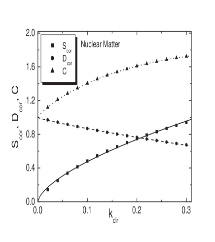
Figure 1: $S_{\rm cor}$, $D_{\rm cor}$ and $C$ of nuclear matter versus the correlation parameter $k_{\rm dir}$. The lines correspond to the expressions (27), (28), (29), with the parameters derived by the least squares fit method.

The calculated values of $S_{\rm cor}$, $D_{\rm cor}$ and $C$ for nuclear matter versus wound parameter $k_{\rm dir}$ are displayed in Fig. 1. $S_{\rm cor}$ and $C$ increase with $k_{\rm dir}$, while $D_{\rm cor}$ decreases. We fitted the numerical values of the above quantities, with simple functions of $k_{\rm dir}$ and we find respectively the following formulae

$$S_{\rm cor}=\alpha k_{\rm dir}^{\beta},\qquad\alpha=2.0586,\quad\beta=0.6365.$$ (27)

$$D_{\rm cor}=1+\alpha k_{\rm dir}^{\beta},\qquad\alpha=-0.9009,\quad\beta=0.8325.$$ (28)

$$C=1+\alpha k_{\rm dir}^{\beta}\textrm{e}^{\gamma k_{\rm dir}},\qquad\alpha=3.1760,\quad\beta=0.8257,\quad\gamma=-1.6176.$$ (29)

The values of the parameters $\alpha$, $\beta$ and $\gamma$, for each case, have been selected by a least squares fit (LSF) method.

Another characteristic quantity, used as a measure of the strength of correlations of the uniform Fermi systems, is the discontinuity, $Z_{F}$, of the momentum distribution at $k/k_{F}=1$. It is defined as

$$Z_{F}=n(1^{-})-n(1^{+})$$

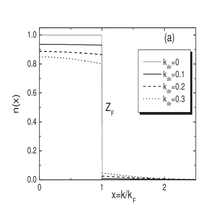
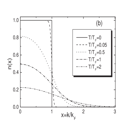
Figure 2: (a) The momentum distribution for correlated nuclear matter versus $k/k_{F}$ for various values of the correlation parameter $k_{\rm dir}$ (b) The momentum distribution of an ideal electron gas versus $k/k_{F}$ for various values of the ratio $T/T_{F}$.

The behavior of momentum distribution, as a function of $k/k_{F}$ for various values of the wound parameter $k_{\rm dir}$ is indicated in Fig. 2(a). The discontinuity $Z_{F}$ is also displayed in each case. For ideal Fermi systems $Z_{F}=1$, while for interacting ones $Z_{F}<1$. In the limit of very strong interaction $Z_{F}=0$, there is no discontinuity on the momentum distribution of the system. The quantity ($1-Z_{F}$) measures the ability of correlations to deplete the Fermi sea by exciting particles from states below it (hole states) to states above it (particle states) [54].

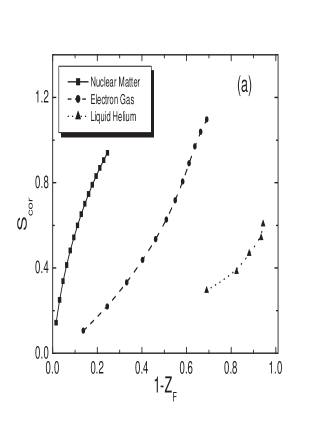
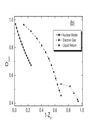
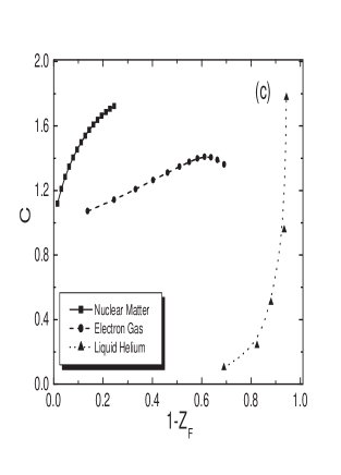
Figure 3: (a) $S_{\rm cor}$ (b) $D_{\rm cor}$ and (c) $C$ for nuclear matter, electron gas and liquid helium versus the discontinuity parameter $(1-Z_{F})$. In the case of liquid helium, the values of $S_{\rm cor}$ are divided by $10$ and the values of $C$ by $100$.

The dependence of $S_{\rm cor}$, $D_{\rm cor}$ and $C$ on the quantity $(1-Z_{F})$ is shown in Fig. 3. It is seen that $S_{\rm cor}$ and $C$ are increasing functions of $(1-Z_{F})$, while $D_{\rm cor}$ is a decreasing one, as a direct consequence of the dependence of the above quantities, on the correlation parameter $k_{\rm dir}$. That dependence can be reproduced very well by simple expressions as in Eqs. (27), (28) and (29) replacing $k_{\rm dir}$ by $(1-Z_{F})$. For example the expression

$$C(Z_{F})=1+\alpha(1-Z_{F})^{\beta}\,\textrm{e}^{\gamma(1-Z_{F})}$$ (30)

with $\alpha=3.6227$, $\beta=0.8024$ and $\gamma=-1.9750$ reproduces the numerical values of $C$ very well.

¿From the above analysis we can conclude that LMC complexity $C$ can be employed as a measure of the strength of correlations in the same way the wound and the discontinuity parameters are used. An explanation of the above behavior of $C$ is the following: The effect of nucleon correlations is the departure from the step function form of the momentum distribution (ideal Fermi gas) to the one with long tail behavior for $k>k_{F}$. The diffusion of the distribution leads to a decrease of the order of the system (the disequilibrium $D_{k}$ decreases and the information entropy $S_{k}$ increases accordingly). In total, the contribution of $S_{k}$ in $C$ dominates over the contribution of $D_{k}$ and thus the complexity increases with the correlations (at least in the region under consideration).

2.2 Electron gas

We consider as electron gas, a system of fermions interacting via a Coulomb potential. The electron gas is a model of conduction electrons in a metal, where the periodic positive potential due to the ions is replaced by a uniform charge distribution. The density of the uniform electron gas (Jellium) is $\rho=3/(4\pi r_{o}^{3})$ and the momentum distribution is $n(x,r_{s})$, a function of both $x=k/k_{F}$ and $r_{s}=r_{o}/a_{B}$ (where $a_{B}=\hbar^{2}/me^{2}$ is the Bohr radius). In the Fermi-liquid regime, the momentum distribution of the unpolarized uniform electron gas $n(x,r_{s})$ is constructed with the help of the convex Kulik function $G(\chi)$ [56].

Discontinuity $Z_{F}(r_{s})$ is unit for $r_{s}=0$ and it is a decreasing function of interaction strength $r_{s}$, as $r_{s}$ increases. The discontinuity gap of the momentum distribution $n(k)$ at the Fermi surface narrows as the density decreases, a clear indication that the system becomes more strongly coupled. That behavior is due to the fact that the screening of the long-range Coulomb interaction between the electrons becomes less effective at lower density. Nuclear matter and atomic ³He exhibit an inverse behavior, where the basic interactions are of short range and $Z_{F}$ decreases as the density increases. At large $r_{s}$, electrons form a Wigner crystal with a smooth $n(x,r_{s})$. Interaction strength $r_{s}\ll 1$ is the weak-correlation limit and $r_{s}\gg 1$ is the strong-correlation limit, respectively. For intermediate values of $r_{s}$, a non-Fermi liquid regime may exist with $Z_{F}=0$ [56].

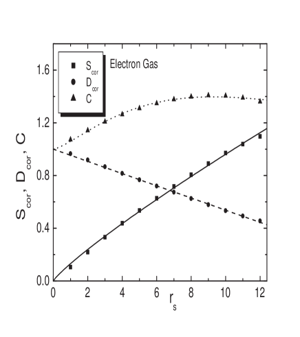
Figure 4: $S_{\rm cor}$, $D_{\rm cor}$ and $C$ of electron gas the correlation parameter $r_{s}$. The lines correspond to the expressions (31), (32), (33), with the parameters derived by the least squares fit method.

We examine the dependence of $S_{\rm cor}$, $D_{\rm cor}$ and $C$ for the electron gas on the correlation parameter $r_{s}$, (or $\rho=3/(4\pi r_{o}^{3})$) and the discontinuity parameter ($1-Z_{F}$). This dependence is displayed in Fig. 4. It is seen that, as in the case of nuclear matter, $S_{cor}$ depends on those quantities through a two parameter expression of the form

$$S_{\rm cor}(r_{s})=\alpha r_{s}^{\beta},\quad\alpha=0.1312,\qquad\beta=0.8648.$$ (31)

The disequilibrium $D_{\rm cor}$ takes the form

$$D_{\rm cor}=1-\alpha r_{s},\qquad\alpha=0.0463,$$ (32)

and the complexity $C$ behaves as

$$C=1+\alpha r_{s}^{\beta}\textrm{e}^{\gamma r_{s}},\qquad\alpha=0.0700,\quad\beta=1.4144,\quad\gamma=-0.1525.$$ (33)

The most distinctive feature, in the case of electron gas, is the occurrence of a maximum of $C$ for high values of the correlations parameter $r_{s}$ in contrast to the case of nuclear matter and liquid helium (see bellow), where $C$ is a monotonic increasing function of correlations. For high values of $r_{s}$, the competition between $D_{\rm cor}$ and $\textrm{e}^{S_{\rm cor}}$ (see Eq. (18)) leads to the dominance of the trend of $D_{\rm cor}$. More precisely the slope of $C$ is given by

$$\frac{dC}{dr_{s}}=C\left(\frac{d\ln D_{\rm cor}}{dr_{s}}+\frac{dS_{\rm cor}}{dr_{s}}\right).$$ (34)

Thus, according to Eq. (34) the sign of the slope of $C$ depends on the sum of the terms $\frac{d\ln D_{\rm cor}}{dr_{s}}$ and $\frac{dS_{\rm cor}}{dr_{s}}$ (which are always negative and positive respectively when $r_{s}$ increases). It is easy to show by applying Eqs. (31) and (32) (or equivalently, but with less accuracy from Eq. (33)) that $C$ attains a maximum value $C_{\rm max}\simeq 1.4052$ at $r_{s}\simeq 9.589$.

The above feature is well reflected also on the $1-Z_{F}$ dependence of $C$ as exhibited in Fig. 3. (the trend of $S_{\rm cor}$ and $D_{\rm cor}$ is also shown).

2.2.1 Momentum distribution and complexity for the Wigner Crystal

In the low-density limit, $r_{s}\rightarrow\infty$, the electron gas undergoes Wigner crystallization. The momentum distribution of the localized electron is of harmonic-oscillator type and has the form

$$n(k,r_{s}\rightarrow\infty)=\left(\frac{1}{z}\frac{1}{\pi k_{F}^{2}}\right)^{3/2}\,\textrm{e}^{-\frac{k^{2}}{k_{F}^{2}}\frac{1}{z}},\qquad 4\pi\int_{0}^{\infty}k^{2}n(k,r_{s}\rightarrow\infty)\textrm{d}k=1,$$ (35)

where $z=\omega/k_{F}^{2}=0.24r_{s}^{1/2}$ [56]. It is easy to prove that after some algebra

$$S_{\rm cor}=\frac{3}{2}+\ln{\frac{3\pi^{1/2}}{4}}+\frac{3}{2}\,\ln{z}.$$ (36)

Additionally, $D_{\rm cor}$ can be found also from the expression

$$D_{\rm cor}=\frac{2^{1/2}}{3\pi^{1/2}}z^{-3/2}.$$ (37)

¿From Eqs. (36), (37) we find that

$$C=\textrm{e}^{S_{\rm cor}}D_{\rm cor}=\left(\frac{\textrm{e}}{2}\right)^{3/2}\simeq 1.5845.$$ (38)

So, in the low-density limit (very strong correlations) the complexity is independent of the correlation parameter $r_{s}$. As we show below the above case is similar to that of an ideal Fermi gas at high values of temperature.

2.3 Liquid ³He

The interaction potential for liquid ³He is very strong at small distances and its core repulsion is very hard (but not infinite). Consequently there is a Fermi surface discontinuity of roughly $Z_{F}\sim 0.3$. This small value supports the view that ³He is the most strongly interacting Fermi system of the three systems considered here. The momentum distribution has been calculated using diffusion Monte Carlo simulations with the use of trial functions optimized via the Euler-Monte Carlo method [55].

We examine the dependence of $S_{\rm cor}$, $D_{\rm cor}$ and $C$ on the density $\rho=3/(4\pi r_{o}^{3})$ and the discontinuity parameter $(1-Z_{F})$, and we present our results in Fig. 5. The dependence of $S_{\rm cor}$ on those parameters is described through the following simple two parameter formula (as in the cases of electron gas and nuclear matter)

$$S_{cor}(\rho_{0})=\alpha\rho_{0}^{\beta},\qquad\rho_{0}=100\rho,$$ (39)

with

$$\alpha=2.2736,\qquad\beta=1.4757,$$

while the disequilibrium $D_{\rm cor}$ is described by the function

$$D_{\rm cor}=\frac{\alpha}{1+\textrm{e}^{(\rho_{0}-\beta)/\gamma}}+\delta,\qquad\alpha=0.1321,\quad\beta=1.6288,\quad\gamma=0.1031,\quad\delta=0.4062.$$ (40)

The complexity $C$ behaves as

$$C=1+\alpha\rho_{0}^{\beta}\,\textrm{e}^{\gamma\rho_{0}},\qquad\alpha=0.0166,\quad\beta=-3.1849,\quad\gamma=5.8556.$$ (41)

The dependence of $S_{\rm cor}$, $D_{\rm cor}$ and $C$ on the quantity $(1-Z_{F})$ is seen in Fig. 3. In order to be able to compare the results of the various systems, in the case of liquid ³He the values of $S_{\rm cor}$ have been divided by $10$ and the values of $C$ by $100$. The most distinctive feature of the above analysis, in the various systems, is the different behavior exhibited by $S_{\rm cor}$, $D_{\rm cor}$ and $C$ as function of $(1-Z_{F})$. For the same values of $(1-Z_{F})$ both the values and the trend of these quantities are different in those systems.

3 Thermal effects on complexity in electron gas

At temperature $T=0$, the electrons of the electron gas occupy all the lower available states up to a highest one, namely the Fermi level. As the temperature increases the electrons of the gas tend to become excited and occupy states of energy of order $kT$ higher than the Fermi energy. In general the occupation number of the electron gas $n(\epsilon)$, is given by the Fermi-Dirac formula

$$n(\epsilon)=\frac{1}{\exp\left[\frac{1}{k_{B}T}\,(\epsilon-\mu)\right]+1},$$ (42)

where $\epsilon=\frac{p^{2}}{2m}$ ($p=\hbar k$) is the energy of the electrons, $k_{B}$ is the Boltzmann’s constant and $\mu$ is the chemical potential. For $T=0$, the chemical potential of a gas coincides with the Fermi energy $\epsilon_{F}$, which is by definition the energy of the highest single-particle level occupied at $T=0$. i.e.

$$\epsilon_{F}=\frac{\hbar^{2}}{2m}\,\left(3\pi^{2}\rho\right)^{2/3},$$ (43)

while the Fermi temperature is defined via the relation

$$\epsilon_{F}=k_{B}T_{F}.$$ (44)

We will examine how information and complexity measures considered in the present study are affected by temperature, when it starts to increase above zero. The limits of low temperature (quantum regime) and high temperature (classical regime) are studied separately in the following subsections.

3.1 Quantum regime ($T\ll T_{F}$)

With the term low energy we refer to the limit $T\ll T_{F}$, since there is only a single characteristic value of temperature, the Fermi temperature. In a first approximation, the chemical potential for that limit, is [58, 59, 60]

$$\mu=\epsilon_{F}\,\left[1-\frac{\pi^{2}}{12}\left(\frac{T}{T_{F}}\right)^{2}\right],$$ (45)

and so Eq. (42) becomes

$$n(x)=\frac{1}{\exp\left[\frac{1}{\xi}\,\left(x^{2}-1+\frac{\pi^{2}}{12}\,\xi^{2}\right)\right]+1},$$ (46)

where $x=(\epsilon/\epsilon_{F})^{1/2}=k/k_{F}$, $\xi=T/T_{F}\ll 1$ and $\int_{0}^{\infty}x^{2}n(x)\,\textrm{d}x=1/3$.

Following the same procedure as in Section II, the information entropy $S_{k}$ of the electron gas at temperature $T\ll T_{F}$ is written

$$S_{k}=S_{0}+S_{\rm thermal},$$ (47)

where $S_{0}$ is given by Eq.(7) and

$$S_{\rm thermal}=-3\int_{0}^{\infty}x^{2}n(x)\ln{n(x)}\,\textrm{d}x.$$ (48)

In a similar way we find that $D_{k}$ is written as

$$D_{k}=D_{0}D_{\rm thermal},$$ (49)

where $D_{0}$ is given in Eq. (12) and $D_{\rm thermal}$ can be calculated also using the expression

$$D_{\rm thermal}=3\int_{0}^{\infty}x^{2}n^{2}(x)\,\textrm{d}x.$$ (50)

Finally, it is easy to show that

$$C=C_{0}C_{cor}=\textrm{e}^{S_{\rm thermal}}\,D_{\rm thermal},\qquad C_{0}=1.$$ (51)

It is worthwhile to notice that the correlations between the Fermi particles invoke a discontinuity to the momentum distribution at $k=k_{F}$ (see Fig. 2(a)), while the thermal effect causes just a slight deviation from the sharp step function form at $T=0$. This is shown in Fig. 2(b), where the momentum distribution for an ideal electron gas, at various values of $T/T_{F}$ has been plotted versus $k/k_{F}$. The origin of the two effects (correlations and temperature) is different and it is seen that they influence in a different way the momentum distribution. So, it may be appropriate to study qualitatively and also quantitatively the above effects on the various information measures and complexity.

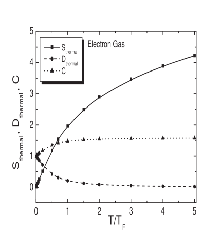
Figure 6: $S_{\rm thermal}$, $D_{\rm thermal}$ and $C$ of an ideal electron gas versus the ratio $T/T_{F}$.

The calculated values of $S_{\rm thermal}$ for various values of the temperature in the low energy limit ($T\ll T_{F}$) are shown in Fig. 6. It is seen that $S_{\rm thermal}$ is an increasing linear function of the temperature. The linear equation

$$S_{\rm thermal}=\alpha\,\frac{T}{T_{F}},\qquad\alpha=2.5466$$ (52)

reproduces very well the calculated values of $S_{thermal}$. That expression of the information entropy is similar to the expression which gives the thermodynamical entropy, $S_{TE}$, for $T\ll T_{F}$. $S_{TE}$ in the low temperature limit has the form [58, 60]

$$S_{TE}=\frac{\pi^{2}}{2}\,Nk_{B}\,\frac{T}{T_{F}}.$$ (53)

¿From Eqs. (52) and (53), we can find a relation between the two entropies in the limit $T\ll T_{F}$. The corresponding relation is of the form

$$S_{\rm thermal}=\frac{2\alpha}{\pi^{2}}\,\frac{S_{TE}}{Nk_{B}}.$$ (54)

The calculated values of $D_{thermal}$, displayed in Fig. 6, are well reproduced by the formula

$$D_{\rm thermal}=\textrm{e}^{-1.647\left(\frac{T}{T_{F}}\right)}.$$ (55)

Finally, the calculated values of $C$ as a function of $T/T_{F}$ are shown in Fig. 6. $C$ is an increasing function of $T/T_{F}$ and exhibits a linear trend which is fairly reproduced by the relation

$$C=1+0.962\,\frac{T}{T_{F}}.$$ (56)

3.2 Classical regime ( $T\gg T_{F}$)

In the classical case (where the density is low and/or the temperature is high and it is assumed that $n(k)\ll 1$) relations can also be established between the information measures and complexity with temperature. In that case the momentum distribution has the gaussian form [59]

$$n(k)=\left(\frac{a}{\pi}\right)^{3/2}\textrm{e}^{-ak^{2}},\qquad a=\frac{\hbar^{2}}{2mk_{B}T},$$ (57)

and is normalized as $\int n(k)\,\textrm{d}{\bf k}=1$. The above expression is also written as

$$n(k)=\left(\frac{1}{\xi}\,\frac{1}{\pi k_{F}^{2}}\right)^{3/2}\textrm{e}^{-\frac{k^{2}}{k_{F}^{2}}\frac{1}{\xi}},\qquad\xi=T/T_{F}.$$ (58)

¿From Eqs. (48) and (58), the following relation, connecting $S_{\rm thermal}$ with the temperature, can be found [16]

$$S_{\rm thermal}=\frac{3}{2}+\ln{\frac{3\pi^{1/2}}{4}}+\frac{3}{2}\,\ln{\frac{T}{T_{F}}}.$$ (59)

Additionally, we can also obtain $D_{\rm thermal}$ from the expression

$$D_{\rm thermal}=\frac{2^{1/2}}{3\pi^{1/2}}\,\left(\frac{T}{T_{F}}\right)^{-3/2}.$$ (60)

¿From Eqs. (59), (60) we find that

$$C=C_{\rm thermal}=\textrm{e}^{S_{\rm thermal}}\,D_{\rm thermal}=\left(\frac{\textrm{e}}{2}\right)^{3/2}\simeq 1.5845.$$ (61)

The physical meaning of Eq. (61) is very clear. For high values of temperature ($T\gg T_{F}$), where the momentum distribution of the gas is described by a Gaussian function, the complexity $C$ is independent of $T$ and takes a constant value. Our finding show that the case of an ideal Fermi gas at $T\gg T_{F}$, is in contrast to the case of correlated Fermi gas at $T=0$, where, in general, $C$ is not an upper bounded function. Moreover, the complexity has different trend in the quantum mechanical limit ($T\rightarrow 0$) compared to the classical limit ($T\rightarrow\infty$). In the classical limit, $C$ is not affected by the temperature variation and is a constant of the system. However, for low values of $T$, complexity exhibits strong temperature dependence.

In Fig. 6 we plot the complexity versus $\xi=T/T_{F}$ both for low and high values of temperature. Actually, we calculate the chemical potential for each value of $\xi$ and consequently, we know exactly the momentum dependence of the occupation numbers given in Eq. (42). The results confirm the numerical approximation of $C$ given in Eq. (56) for low values of $\xi$ as well as the analytical prediction of Eq. (61) for high values of $\xi$.

It is worthwhile to notice that the temperature dependence of $C$ is similar to that of the specific heat $C_{V}$ in an ideal Fermi gas [60]. More precisely, $C_{V}$ is a linear function of $T$ for $T\ll T_{F}$, while it approaches $3/2Nk_{B}$ as $T\rightarrow\infty$ [60]. In order to illustrate the above result we display in Fig. 7 the dependence of $C$ and the specific heat $C_{V}$ on $T$ (in units $T_{F}$). This behavior can be explained as follows: Let us consider two momentum distributions $n(k)$, one for $T=0$ and another one for $T>0$. They are in essence different, because for $T>0$ a certain number of fermions are excited above the Fermi level $\epsilon_{F}$. Specifically, fermions with energies of the order of $k_{B}T$ below $\epsilon_{F}$ are excited to energies of the order of $k_{B}T$ above $\epsilon_{F}$. However, this holds only for fermions with energies within about $k_{B}T$ of the Fermi level, while those with other values of energy have no place to go –the states are occupied [61].

To sum up, thermal effects lead to a blurring of the Fermi surface that means the distribution function $n(\epsilon)$ drops over the range $\epsilon_{F}\pm k_{B}T$. As a consequence, in the case of low temperature limit, only the momentum distribution (or the occupation number) close to the Fermi surface is affected by $T$ and this leads to a linear dependence of $C$ on $T$. For $T\gg T_{F}$, the momentum distribution is affected for both low and high values of $k$ in such a way so that the complexity $C$ tends to a constant.

4 Conclusions

In the present work the recently proposed statistical measure of complexity $C$ has been an issue under consideration. Information theoretical measures (information entropy and disequilibrium) as well as a statistical measure of complexity $C$ have been calculated, in momentum space, for realistic Fermi systems, that is nuclear matter, electron gas and liquid helium. The dependence of the above measures on the strength of the correlations has been analyzed and displayed. From the present analysis it should become clear that the values of the above quantities could be used as a measure of the particle correlations of Fermi systems. We have found that the complexity is an increasing function of the correlations both for nuclear matter and liquid helium as expected intuitively. However, in the case of electron gas, complexity exhibits a different slope and in fact, the function of $C(r_{s})$ has a maximum for a specific value of the correlation parameter $r_{s}$. Additionally, we have found the interesting result that for very strong correlations, where electron gas undergoes Wigner crystallization, the complexity is independent of the correlations and takes a constant value. In order to have a common measure of the various information properties, we have displayed them as a function of the discontinuity gap, $(1-Z_{F})$. The most distinctive feature of the above analysis, in the various systems, is the different behavior exhibited by $S_{\rm cor}$, $D_{\rm cor}$ and $C$ as functions of $(1-Z_{F})$. For the same values of $(1-Z_{F})$ both the values and the trend of these quantities are different in the various systems. Considering that, under certain circumstances, $Z_{F}$ can be estimated experimentally, we obtain a first indication that information properties may be related with experimental results.

Temperature also affects the momentum distribution of an ideal Fermi gas and consequently all the related information properties. We have found that for low values of the ratio $T/T_{F}$ the complexity is a linear function of $T$. However, in the high temperature limit (the well known classical Maxwell-Boltzmann distribution), complexity is independent of $T$ and takes a fixed value (exactly the same as in the case of Wigner crystallization). Thus, regardless of the reason that causes the momentum distribution to exhibit gaussian type dependence on the momenta $k$, the value of the complexity is constant. Furthermore, we have seen that the temperature dependence of $C$ is similar to that of the specific heat $C_{V}$ in an ideal Fermi-gas [60], both for low and high values of $T$. This is a second indication that one can relate the statistical measure of complexity $C$ with experimental data (as the specific heat $C_{V}$). However, further work is called for before we establish a clear connection between information theoretical measures and experimental data.

As an epilogue, we would like to mention that physicists have been carrying out research for decades, going beyond the mean-field description of quantum many-body systems, by taking into account correlations among particles, a very important factor indeed towards a better understanding of these systems. The effect of correlations is connected intuitively with the concept of complexity, in a qualitative, and somehow vague way. The present work contributes to a quantification of complexity $C$ in correlated Fermi systems, based on previous research for the information entropy of the same systems [16]. It turns out that $C(T)$ and the specific heat $C_{V}(T)$ are similar functions of the temperature $T$ as seen in Fig 7(a). In Fig. 7(b) we plot $C_{V}(C)$. The dependence of $C_{V}$ on $C$ is approximately linear. In fact there appear two regions of linear dependence with a different slope, separated by a cross. The fitted expressions are $C_{V}=-1.7353+1.7114C$ (region A) and $C_{V}=-6.3777+5.0783C$ (region B). In a sense, one may state that $C_{V}(T)$ can serve as an index reflecting the expected increase of complexity as $T$ increases. Furthermore, it is seen that for temperatures $T\gg T_{F}$ complexity reaches a plateau (saturation) i.e. it can no longer increase. The textbook definition of the specific heat is the measure of heat energy required to increase the temperature of a unit of quantity of a substance by a unit degree. It is noted that here, we observe an empirical connection of such an ”energy-like” quantity with complexity $C$ calculated employing information entropy, which is not related directly to the energy of the system in contrast to the traditional concept of thermodynamic entropy.

Figure 5: $S_{\rm cor}$, $D_{\rm cor}$ and $C$ of liquid helium versus the correlation parameter $\rho_{0}$. The values of $S_{\rm cor}$ are divided by $10$ and the values of $C$ by $100$. The lines correspond to the expressions (39), (40), (41), with the parameters derived by the least squares fit method.

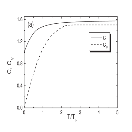
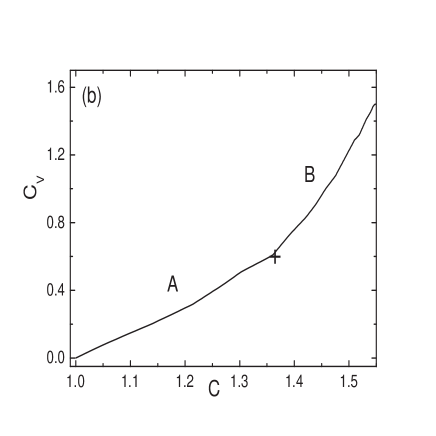
Figure 7: (a) The complexity $C$ and the specific heat $C_{V}$ (in units $k_{B}N$) of an ideal electron gas versus the ratio $T/T_{F}$ (b) The specific heat $C_{V}$ versus complexity $C$.

References

- [1] C.E. Shannon, Bell Syst. Tech. J. 27, 379 (1948).
- [2] S.R. Gadre, Phys. Rev. A 30, 620 (1984); S.R. Gadre, S.B. Sears, S.J. Chakravorty, and R.D. Bendale, Phys. Rev. A 32, 2602 (1985); S.R. Gadre and R.D. Bendale, Phys. Rev. A 36, 1932 (1987).
- [3] O. Onicescu, Theorie de l information. Energie informationelle., Vol. 263 of A, C. R. Acad. Sci. Paris, 1966.
- [4] I. Bialynicki-Birula and J. Mycielski, Commun. Math. Phys. 44, (1975) 129.
- [5] R.A. Fisher, Proc. Cambridge Phil. Sec. 22, 700 (1925).
- [6] S. Kullback, Statistics and Information theory, (Wiley, New York, 1959).
- [7] M. Ohya and P. Petz, ”Quantum entropy and its use” (Springer Berlin, 1993).
- [8] V. Zelevinsky, M. Horoi, and B.A. Brown, Phys. Lett. B 350, 141 (1995). V.V. Sokolov, B.A. Brown, and V. Zelevinsky, Phys. Rev E 58, 56 (1998).
- [9] A. Nagy and R.G. Parr, Int. J. Quant. Chem. 58, 323 (1996).
- [10] V. Majernic and T. Opatrny, J. Phys. A 29, 2187 (1996).
- [11] C.P. Panos and S.E. Massen, Int.J. Mod. Phys. E 6, 497 (1997); G.A. Lalazissis, S.E. Massen, C.P. Panos, and S.S. Dimitrova, Int. J. Mod. Phys. E 7, 485 (1998).
- [12] S.E. Massen and C.P. Panos, Phys. Lett. A 246, 530 (1998); S.E. Massen and C.P. Panos, Phys. Lett. A 280, 65 (2001); S.E. Massen, Ch.C. Moustakidis, and C.P. Panos, Phys. Lett A 289, 131 (2002); C.P. Panos, Phys. Lett. A 289, 287 (2001).
- [13] S.K. Ghosh, M. Berkowitz, and R.G. Parr, Proc. Natl. Acad. Sc. USA 81, 8028 (1984).
- [14] P. Garbaczewski, J. Stat. Phys. 123, 315 (2006).
- [15] B.R. Frieden, Science from Fisher Information, (Cambridge University Press, 2004).
- [16] Ch.C. Moustakidis and S.E. Massen, Phys. Rev. B 71, 045102 (2005).
- [17] S.H. Patil, K.D. Sen, N.A. Watson, and H.E. Montogomery, J. Phys. B 40, 2147 (2007).
- [18] S.B. Liu, J. Chem. Phys. 126, 191107 (2007).
- [19] A.V. Luzanov and O.V. Prezhdo, Mol. Phys. 105, 2879 (2007).
- [20] J. Antolín and J.C. Angulo, Eur. Phys. J. D 46, 21 (2008).
- [21] R.P. Sagar and N.L. Guevara, J. Mol. Struct. (Theochem) 857, 72 (2008).
- [22] R. López-Ruiz, H.L. Mancini, and X. Calbet, Phys. Lett. A 209, 321 (1995).
- [23] R.G. Catalán, J. Garay, and R. López-Ruiz, Phys. Rev. E 66, 011102 (2002).
- [24] J. Sañudo and A.F. Pacheco, Phys. Lett. A 373, 807 (2009).
- [25] P.T. Landsberg and J.S. Shiner, Phys. Lett. A 245, 228 (1998); P.T. Landsberg, Phys. Lett. A 102, 171 (1984).
- [26] J.S. Shiner, M. Davison, and P.T. Landsberg, Phys. Rev. E 59, 1459 (1999).
- [27] D.P. Feldman and J.P. Crutchfield, Phys. Lett. A 238, 244 (1998).
- [28] J.P. Crutchfield, D.P. Feldman, and C.R. Shalizi, Phys. Rev. E 62, 2996 (2000).
- [29] P.M. Binder and N. Perry, Phys. Rev. E 62, 2998 (2000).
- [30] K.Ch. Chatzisavvas, Ch.C. Moustakidis, and C.P. Panos, J. Chem. Phys. 123, 174111 (2005).
- [31] M.T. Martin, A. Plastino, and O.A. Rosso, Phys. Lett. A 311, 126 (2003).
- [32] K.D. Sen, C.P. Panos, K.Ch. Chatzisavvas, and Ch.C. Moustakidis, Phys. Lett. A 364, 286 (2007).
- [33] C.P. Panos, K.Ch. Chatzisavvas, Ch.C. Moustakidis, and E.G. Kyrkou, Phys. Lett. A 363, 78 (2007).
- [34] C.P. Panos, N.S. Nikolaidis, K.Ch. Chatzisavvas, and C.C. Tsouros, Phys. Lett. A 373, 2343 (2009).
- [35] R. López-Ruiz, Biophys. Chem. 115, 215 (2005).
- [36] T. Yamano, J. Math. Phys. 45, 1974 (2004).
- [37] C. Anteneodo and and A.R. Plastino, Phys. Lett. A 223, 348 (1996).
- [38] A. Borgoo, F. De Proft, P. Geerlings, and K.D. Sen, Chem. Phys. Lett. 444, 186 (2007).
- [39] H.E. Montgomery and K.D. Sen, Phys. Lett. A 372, 2271 (2008).
- [40] X. Calbet and R. López-Ruiz, Physica A 382, 523 (2007).
- [41] J.C. Angulo and J. Antolín, J. Chem. Phys. 128, 164109 (2008).
- [42] J.C. Angulo, J. Antolín, and K.D. Sen, Phys. Lett. A 372, 670 (2008).
- [43] J. Sañudo and R. López-Ruiz, Phys. Lett. A 372, 5283 (2008).
- [44] J. Sañudo and R. López-Ruiz, J. Phys. A 41, 265303 (2008).
- [45] K.Ch. Chatzisavvas, V.P. Psonis, C.P. Panos, and Ch.C. Moustakidis, Phys. Lett. A 373, 3901 (2009).
- [46] S. López-Rosa, D. Manzano, and J.S. Dehesa, Physica A 388, 3273 (2009).
- [47] R. López-Ruiz, A. Nagy, E. Romera, and J. Sañudo, e-print arXiv: 0905.3360.
- [48] S. López-Rosa, D. Manzano, and J.S. Dehesa, e-print arXiv: 0907.0570.
- [49] A. Rényi On measures of information and entropy, Proceedings of the 4th Berkeley Symposium on Mathematics, Statistics and Probability 1960, pp. 547-561 (1961).
- [50] J. Antolín, S. Lopéz-Rosa, J.C. Angulo, Chem. Phys. Lett. 474 233 (2009).
- [51] A.B. Migdal, Theory of Finite Fermi-Systems and Applications to Atomic Nuclei (Wiley Interscience, New York, 1967).
- [52] M. Gaudin, J. Gillespie, and G. Ripka, Nucl. Phys. A176, 237 (1971).
- [53] M. Dal Ri, S. Stringari, and O. Bohigas, Nucl. Phys. A376, 81 (1982).
- [54] M.F. Flynn, J.W. Clark, R.M. Panoff, O. Bohigas, and S. Stringari, Nucl. Phys. A427, 253 (1984).
- [55] S. Moroni, G. Senatore and S. Fantoni, Phys. Rev. B 55, 1040 (1997).
- [56] P. Gori-Giorgi and P. Ziesche, Phys. Rev. B 66, 235116 (2002).
- [57] R. Jastrow, Phys. Rev. 98, 1479 (1955).
- [58] D.L. Goodstein, States of Matter (Dover Publications, Inc, New York, 1985).
- [59] F. Mandl, Statistical Physics (John Wiley, New York, 1978).
- [60] K. Huang, Statistical Mechanics (John Wiley, New York, 1987).
- [61] R.P. Feynman, Statistical Mechanics (Addison-Wesley, Reading, MA, 1972).