Sparsistent Estimation Of Time-Varying Markov Random Fields

Abstract

Network models have been popular for modeling and representing complex relationships and dependencies between observed variables. When data comes from a dynamic stochastic process, a single static network model cannot adequately capture transient dependencies, such as, gene regulatory dependencies throughout a developmental cycle of an organism. Kolar et al (2010b) proposed a method based on kernel-smoothing l1-penalized logistic regression for estimating time-varying networks from nodal observations collected from a time-series of observational data. In this paper, we establish conditions under which the proposed method consistently recovers the structure of a time-varying network. This work complements previous empirical findings by providing sound theoretical guarantees for the proposed estimation procedure. For completeness, we include numerical simulations in the paper.

Key words and phrases: High-dimensional inference, Markov random fields, semi-parametric inference, time-varying Ising model, varying coefficient models.

1 Introduction

In recent years, we have witnessed fast advancement of data-acquisition techniques in many areas, including biological domains, engineering and social sciences. As a result, new statistical and machine learning techniques are needed to help us develop a better understanding of complexities underlying large, noisy data sets. Networks have been commonly used to abstract noisy data and provide an insight into regularities and dependencies between observed variables. For example, in a biological study, nodes of the network can represent genes in one organism and edges can represent associations or regulatory dependencies among genes. In a social domain, nodes of a network can represent actors and edges can represent interactions between actors. Recent popular techniques for modeling and exploring networks are based on the structure estimation in the probabilistic graphical models, specifically, Markov Random Fields (MRFs). These models represent conditional independence between variables, which are represented as nodes. Once the structure of the MRF is estimated, the network is drawn by connecting variables that are conditionally dependent.

Classical literature mainly focuses on estimating a single static network underlying a complex system. However, in reality, many systems are inherently dynamic and can be better explained by a dynamic network whose structure evolves over time. Consider the following real world problems:

• Analysis of gene regulatory networks. Suppose that we have a set of $n$ microarray measurements of gene expression levels, obtained at different stages during the development of an organism or at different times during the cell cycle. Given this data, biologists would like to get insight into dynamic relationships between different genes and how these relations change at different stages of development. The problem is that at each time point there is only one or at most a few measurements of the gene expressions; and a naive approach to estimating the gene regulatory network, which uses only the data at the time point in question to infer the network, would fail. To obtain a good estimate of the regulatory network at any time point, we need to leverage the data collected at other time points and extract some information from them.

• Analysis of stock market. In a finance setting, we have values of different stocks at each time point. Suppose, for simplicity, that we only measure whether the value of a particular stock is going up or down. We would like to find the underlying transient relational patterns between different stocks from these measurements and get insight into how these patterns change over time. Again, we only have one measurement at each time point and we need to leverage information from the data obtained at nearby time points.

• Understanding social networks. There are 100 Senators in the U.S. Senate and each can cast a vote on different bills. Suppose that we are given $n$ voting records over some period of time. How can one infer the latent political liaisons and coalitions among different senators and the way these relationships change with respect to time and with respect to different issues raised in bills just from the voting records?

The aforementioned problems have commonality in estimating a sequence of time-specific latent relational structures between a fixed set of entities (i.e., variables), from a time series of observation data of entities states; and the relational structures between the entities are time evolving, rather than being invariant throughout the data collection period as commonly assumed in much of the current literature on high-dimensional undirected network estimation (see, e.g., Meinshausen and Bühlmann (2006), Bresler et al. (2007), Yuan and Lin (2007), Banerjee et al. (2008), Rothman et al. (2008), Friedman et al. (2008), Ravikumar et al. (2008), Fan et al. (2009), Peng et al. (2009), Ravikumar et al. (2010), Wang et al. (2009), Guo et al. (2010a) and references therein). Typically, the available data for the problem are very scarce, with only one or at most a few measurements corresponding to any particular latent structure, while the total number of potential relations is large and exceeds the total number of observations. However, as we will show later, under the assumption that the network is sparse and slowly changes with time, it is possible to consistently estimate the network structure at any time point.

A popular model for the relational structure over a fixed set of entities that is widely studied is the Markov random field (MRF) (Wainwright and Jordan, 2008, Getoor and Taskar, 2007). Let $G=(V,E)$ represent a graph, of which $V$ denotes the set of vertices, and $E$ denotes the set of edges over vertices. Depending on the specific application of interest, a node $u\in V$ can represent a gene, a stock, or a social actor, and an edge $(u,v)\in E$ can represent a relationship (e.g., correlation, influence, friendship) between actors $u$ and $v$. Let $\mathbf{X}=(X_{1},\ldots,X_{p})^{\prime}$, where $p=|V|$, be a random vector of nodal states following a probability distribution indexed by $\bm{\theta}\in\Theta$. Under a MRF, the nodal states $X_{u}$’s are assumed to be discrete, i.e., $X_{u}\in{\cal X}\equiv\{s_{1},\ldots,s_{k}\}$, and the edge set $E\subseteq V\times V$ encodes certain conditional independence assumptions among components of the random vector $\mathbf{X}$, for example, the random variable $X_{u}$ is conditionally independent of the random variable $X_{v}$ given the rest of the variables if $(u,v)\not\in E$. Under the special case of binary nodal states, e.g., $X_{u}\in{\cal X}\equiv\{-1,1\}$, and assuming pairwise potential weighted by $\theta_{uv}$ for all $(u,v)\in E$ and $\theta_{uv}=0$ for all $(u,v)\not\in E$, the joint probability of $\mathbf{X}=\mathbf{x}$ can be expressed by a simple exponential family model: $\mathbb{P}_{\bm{\theta}}(\mathbf{x})=\frac{1}{Z}\exp\{\sum_{u<v}\theta_{uv}x_{u}x_{v}\}$, also known as the Ising model, where $Z$ denotes the partition function that is usually intractable to compute. A statistical challenge is to estimate the network topology determined by the edge set $E$ from the observed data $\mathbf{x}^{i}\stackrel{{\scriptstyle{iid}}}{{\sim}}\mathbb{P}_{\bm{\theta}}$ $(i=1,\ldots,n)$ with $n\ll p$.

In this paper, we study the problem of estimating a sequence of high-dimensional MRFs that slowly evolve over time from observational data. Suppose that we are given the data $\{\mathbf{x}^{t}\sim\mathbb{P}_{\bm{\theta}^{t}}\}_{t\in{\cal T}_{n}}$, where ${\cal T}_{n}=\{1/n,2/n,\ldots,1\}$ is the time index set, then our goal is to estimate the sequence of graphs $\{G^{t}\}_{t\in{\cal T}_{n}}$ underlying each observation $\mathbf{x}^{t}\sim\mathbb{P}_{\bm{\theta}^{t}}$ in the time series. In order to make this estimation problem feasible, we will have to assume that the underlying probability distribution changes smoothly, which we define precisely later. Estimating a sequence of graphs provides us with insight into the dynamics of the relational changes underlying data. A reader should observe that commonly used methods, which try to estimate a single static graph $G$ from data $\{\mathbf{x}^{i}\}_{i}$ assumed to be i.i.d. from $\mathbb{P}_{\bm{\theta}}$, cannot provide insight into dynamic aspect of the underlying relational structure.

The main contribution of this paper is to establish theoretical guarantees for the estimation procedure for time-varying networks proposed in Kolar et al. (2010b). The estimation procedure is based on temporally smoothed $\ell_{1}$-regularized logistic regression formalism, which is detailed in Section 3. An application to real world data was given in (Song et al., 2009a), where the procedure was used to infer the latent evolving regulatory network underlying 588 genes across the life cycle of Drosophila melanogaster from microarray time course. Although the true regulatory network is not known for this organism, the procedure recovers a number of interactions that were previously experimentally validated. Since in most real world problems the ground truth is not known, we emphasize the importance of simulation studies to evaluate the estimation procedure.

It is noteworthy that the problem of the graph structure estimation is quite different from the problem of (value-) consistent estimation of the unknown parameter $\bm{\theta}$ that indexes the distribution. In general, the graph structure estimation requires a more stringent assumptions on the underlying distribution and the parameter values. For example, observe that a consistent estimator of $\bm{\theta}$ in the Euclidean distance does not guarantee a consistent estimation of the graph structure, encoded by the non-zero patter of the estimator. In the motivating problems that we started with, the main goal is to understand the interactions between different actors. These interactions are more easily interpreted by a domain expert than the numerical values of the parameter vector $\bm{\theta}$ and have potential to reveal more information about the underlying process of interest. This is especially true in situations where there is little or no domain knowledge and one is interested in obtaining casual, preliminary information.

Due to its importance in number of domains, including systems biology, finance and signal processing, a number of authors have proposed algorithms for inferring time inhomogeneous networks, many of which have appeared after the initial draft of this paper was communicated (Kolar and Xing, 2009). The literature can be divided into two categories: estimation of directed graphical models and estimation of undirected graphical models. Literature on estimating time-inhomogeneous directed networks usually assumes a time-varying vector auto-regressive model for observed data (see, for example, Punskaya et al., 2002, Fujita et al., 2007, Rao et al., 2007, Grzegorczyk and Husmeier, 2009, Song et al., 2009b, Robinson and Hartemink, 2009, 2010, Jia and Huan, 2010, Lebre et al., 2010, Husmeier et al., 2010, Dondelinger et al., 2010, Grzegorczyk and Husmeier, 2011b, a, Wang et al., 2011, Grzegorczyk and Husmeier, 2012b, a, Dondelinger et al., 2012, Lebre et al., 2012), a class of models that can be represented in the formalism of time-inhomogeneous Dynamic Bayesian Networks although not all authors use terminology commonly used in the Dynamic Bayesian Networks literature. Markov switching linear dynamical systems are another popular choice for modeling non-stationary time series (see, for example, Andrieu et al., 2003, Yoshida et al., 2005, Dobigeon et al., 2007, Siracusa and Fisher, 2009, Fox et al., 2011, H. Jiang, 2012). This body of work has focused on developing flexible models capable of capturing different assumptions on the underlying system, efficient algorithms and sampling schemes for fitting these models. Although a lot of work has been done in this area, little is known about finite sample and asymptotic properties regarding the consistent recovery of the underlying networks structures. Some asymptotic results are given in Song et al. (2009b). Due to the complexity of MCMC sampling procedures, existing work does not handle well networks with hundreds of nodes, which commonly arise in practice. Finally, the biggest difference from our work is that the estimated networks are directed. Vogel and Fried (2010) point our that undirected models constitute the simplest class of models, whose understanding is crucial for the study of directed models and models with both, directed and undirected edges. Talih and Hengartner (2005) and Xuan and Murphy (2007) study estimation of time-varying Gaussian graphical models in a Bayesian setting. Talih and Hengartner (2005) use a reversible jump MCMC approach to estimate the time-varying variance structure of the data. Xuan and Murphy (2007) proposed an iterative procedure to segment the time-series using the dynamic programming approach developed by Fearnhead (2006) and fit a Gaussian graphical model using the penalized maximum likelihood approach on each segment. To the best of our knowledge, Zhou et al. (2008) is the first work that focuses on consistent estimation, in the Frobenius norm, of covariance and concentration matrix under the assumption that the time-varying Gaussian graphical model changes smoothly over time. Network estimation consistency for this smoothly changing model is established in Kolar and Xing (2011). Time-varying Gaussian graphical models with abrupt changes in network structure were studied in Kolar and Xing (2010), where consistent network recovery is established using a completely different proof technique. A related problem is that of estimating conditional covariance matrices (Yin et al., 2010, Kolar et al., 2010a), where in place of time, which is deterministic quantity, one has a random quantity. Methods for estimating time-varying discrete Markov random fields were given in Ahmed and Xing (2009) and Kolar et al. (2010b), however, no results on the consistency of the network structure were given. As we will see later, showing that a time-varying discrete undirected network is consistently estimated is a much harder task than showing the same result for time-varying Gaussian graphical models.

This paper is organized as follows. Section 2 introduces the network model. The estimation procedure is reviewed in Section 3. The conditions under which the estimation procedure consistently recovers the network structure are stated in Section 4, together with the main theoretical result. The proof is outlined in Section 5 with technical details presented in the appendix. Simulation results are given in Section 6.

2 The Model

We are given a sequence of $n$ nodal states $\mathcal{D}_{n}=\{\mathbf{x}^{t}\sim\mathbb{P}_{\bm{\theta}^{t}}|t\in\mathcal{T}_{n}\}$, with the time index defined as $\mathcal{T}_{n}=\{1/n,2/n,\ldots,1\}$. For simplicity of presentation, we will assume that the observations are equidistant in time and only one observation is available at each time point from distribution $\mathbb{P}_{\bm{\theta}^{t}}$ indexed by $\bm{\theta}^{t}$. Specifically, we assume that the $p$-dimensional random vector $\mathbf{X}^{t}$ takes values in $\{-1,1\}^{p}$ and the probability distribution takes the following form:

$$\mathbb{P}_{\bm{\theta}^{t}}(x)=\frac{1}{Z(\bm{\theta}^{t})}\exp\left(\sum_{(u,v)\in E^{t}}\theta_{uv}^{t}x_{u}x_{v}\right),\quad\forall t\in\mathcal{T}_{n},$$ (2.1)

where $Z(\bm{\theta}^{t})$ is the partition function, $\bm{\theta}^{t}\in\mathbb{R}^{p\choose 2}$ is the parameter vector and $G^{t}=(V,E^{t})$ is an undirected graph representing certain conditional independence assumptions among subsets of the $p$-dimensional random vector $\mathbf{X}^{t}$. For any given time point $\tau\in[0,1]$, we are interested in estimating the graph $G^{\tau}$ associated with $\mathbb{P}_{\bm{\theta}^{\tau}}$, given the observations $\mathcal{D}_{n}$.

Since we are primarily interested in a situation where the total number of observation $n$ is small compared to the dimension $p$, our estimation task is going to be feasible only under some regularity conditions. We impose two natural assumptions: the sparsity of the graphs $\{G^{t}\}_{t\in\mathcal{T}_{n}}$, and the smoothness of the parameters $\bm{\theta}^{t}$ as functions of time. These assumptions are precisely stated in Section 4. Intuitively, the smoothness assumption is required so that a graph structure at the time point $\tau$ can be estimated from samples close in time to $\tau$. On the other hand, the sparsity assumption is required to avoid the curse of dimensionality and to ensure that a the graph structure can be identified from a small sample.

The model given in Eq. (2.1) can be thought of as a nonparametric extension of conventional MRFs, in the similar way as the varying-coefficient models (Cleveland et al., 1991, Hastie and Tibshirani, 1993) are thought of as an extension to the linear regression models. The difference between the model given in Eq. (2.1) and an MRF model is that our model allows for parameters to change, while in MRF the parameters are considered fixed. Allowing parameters to vary over time increases the expressiveness of the model, and make it more suitable for longitudinal network data. For simplicity of presentation, in this paper we consider time-varying MRFs with only pairwise potentials as in Eq. (2.1). Note that in the case of discrete MRFs there is no loss of generality by considering only pairwise interactions, since any MRF with higher-order interactions can be represented with an equivalent MRF with pairwise interactions (Wainwright and Jordan, 2008).

3 Estimation Procedure

In this section, we review the estimation procedure of Kolar et al. (2010b). Given a time point $\tau\in[0,1]$ and a sequence of observations $\mathcal{D}_{n}=\{\mathbf{x}^{t}\sim\mathbb{P}_{\bm{\theta}^{t}}|t\in\mathcal{T}_{n}\}$ with $\mathbb{P}_{\bm{\theta}^{t}}$ defined Eq. (2.1), the goal is to estimate the graph structure of the Markov random field associated with the distribution $\mathbb{P}_{\bm{\theta}^{\tau}}$. The parameter vector $\bm{\theta}^{\tau}$ is a ${p\choose 2}$-dimensional vector, indexed by distinct pairs of nodes, of which an element is non-zero if and only if the corresponding edge $(u,v)\in E^{\tau}$. The problem of recovering the graph structure $G^{\tau}$ is equivalent to estimating the non-zero pattern of the vector $\bm{\theta}^{\tau}$, i.e., locations of non-zero elements of $\bm{\theta}^{\tau}$. A stronger notion of structure estimation is that of signed edge recovery in which an edge $(u,v)\in E^{\tau}$ is recovered together with the sign of the parameter $\operatorname*{sign}(\theta_{uv}^{\tau})$. We will show that the estimation procedure can consistently recover signed edges.

The estimation procedure is based on the neighborhood selection technique, where the graph structure is estimated by combining the local estimates of neighborhoods of each node. For each vertex $u\in V$, define the set of neighboring edges $S^{\tau}(u):=\{(u,v)\ :\ (u,v)\in E^{\tau}\}$ and the set of signed neighboring edges $S^{\tau}_{\pm}(u):=\{(\operatorname*{sign}(\theta_{uv}^{\tau}),(u,v))\ :\ (u,v)\in S^{\tau}(u)\}$. The set of signed neighboring edges $S^{\tau}_{\pm}(u)$ can be determined from the signs of elements of the $(p-1)$-dimensional subvector of parameters $\bm{\theta}_{u}^{\tau}:=\{\theta_{uv}^{\tau}\ :\ v\in V\backslash u\}$ associated with vertex $u$. Under the model (2.1), the conditional distribution of $X_{u}^{\tau}$ given other variables $\mathbf{X}_{\backslash u}^{\tau}:=\{X_{v}^{\tau}\ :\ v\in V\backslash u\}$ takes the form

$$\mathbb{P}_{\bm{\theta}_{u}^{\tau}}(x_{u}^{\tau}|\mathbf{X}_{\backslash u}^{\tau}=\mathbf{x}_{\backslash u}^{\tau})=\frac{\exp(2x_{u}^{\tau}\langle\bm{\theta}_{u}^{\tau},\mathbf{x}_{\backslash u}^{\tau}\rangle)}{\exp(2x_{u}^{\tau}\langle\bm{\theta}_{u}^{\tau},\mathbf{x}_{\backslash u}^{\tau}\rangle)+1},$$ (3.1)

where $\langle a,b\rangle=a^{\prime}b$ denotes the dot product. Observe that the model given in (3.1) can be viewed as expressing $X_{u}^{\tau}$ as the response variable in the generalized varying-coefficient models with $\mathbf{X}_{\backslash u}^{\tau}$ playing the role of covariates. For simplicity, we will write $\mathbb{P}_{\bm{\theta}_{u}^{\tau}}(x_{u}^{\tau}|\mathbf{X}_{\backslash u}^{\tau}=\mathbf{x}_{\backslash u}^{\tau})$ as $\mathbb{P}_{\bm{\theta}_{u}^{\tau}}(x_{u}^{\tau}|\mathbf{x}_{\backslash u}^{\tau})$.

Under the model given in Eq. (3.1) the log-likelihood, for one data-point $t\in{\cal T}_{n}$, can be written in the following form:

$$\gamma(\bm{\theta}_{u};\mathbf{x}^{t}) =\log\mathbb{P}_{\bm{\theta}_{u}}(x_{u}^{t}|\mathbf{x}_{\backslash u}^{t})$$ (3.2)

$$=x_{u}^{t}\langle\bm{\theta}_{u},\mathbf{x}_{\backslash u}^{t}\rangle-\log\left(\exp(\langle\bm{\theta}_{u},\mathbf{x}_{\backslash u}^{t}\rangle)+\exp(-\langle\bm{\theta}_{u},\mathbf{x}_{\backslash u}^{t}\rangle)\right).$$

For an arbitrary point of interest $\tau\in[0,1]$, the estimator $\hat{\bm{\theta}}_{u}^{\tau}$ of the sign-pattern of the vector $\bm{\theta}_{u}^{\tau}$ is defined as the solution to the following convex program:

$$\hat{\bm{\theta}}_{u}^{\tau}=\min_{\bm{\theta}_{u}\in\mathbb{R}^{p-1}}\left\{\ell\left(\bm{\theta}_{u};\mathcal{D}_{n}\right)+\lambda_{n}||\bm{\theta}_{u}||_{1}\right\}$$ (3.3)

where $\ell(\bm{\theta}_{u};\mathcal{D}_{n})=-\sum_{t\in\mathcal{T}_{n}}w_{t}^{\tau}\gamma(\bm{\theta}_{u};\mathbf{x}^{t})$ is the weighted logloss, with weights defined as

$$w_{t}^{\tau}=\frac{K_{h}(t-\tau)}{\sum_{t^{\prime}\in\mathcal{T}_{n}}K_{h}(t^{\prime}-\tau)}$$

and $K_{h}(\cdot)=K(\cdot/h)$ is a symmetric nonnegative kernel. The regularization parameter $\lambda_{n}\geq 0$ is specified by a user and controls the sparsity of the solution. The program (3.3) is convex and a minimum over $\bm{\theta}_{u}$ is always achieved, as the problem can be cast as a constrained optimization problem over the ball $||\bm{\theta}_{u}||_{1}\leq C(\lambda_{n})$ and the claim follows from the Weierstrass theorem.

Let $\hat{\bm{\theta}}_{u}^{\tau}$ be a minimizer of (3.3). The convex program (3.3) does not necessarily have a unique optimum, but as we will prove shortly, in the regime of interest any two solutions will have non-zero elements in the same positions. Based on the vector $\hat{\bm{\theta}}_{u}^{\tau}$, we have the following estimate of the signed neighborhood:

$$\hat{S}^{\tau}_{\pm}(u):=\left\{(\operatorname*{sign}(\hat{\theta}^{\tau}_{uv}),(u,v))\ :\ v\in V\backslash u,\ \hat{\theta}^{\tau}_{uv}\neq 0\right\}.$$ (3.4)

The structure of graph $G^{\tau}$ is consistently estimated if every signed neighborhood is recovered, i.e. $\hat{S}_{\pm}^{\tau}(u)=S_{\pm}^{\tau}(u)$ for all $u\in V$. A summary of the algorithm is given in Algorithm 1.

Algorithm 1 Graph structure estimation

Input: Dataset $\mathcal{D}_{n}$, time point of interest $\tau\in[0,1]$, penalty parameter $\lambda_{n}$, bandwidth parameter $h$
Output: Estimate of the graph structure $\hat{G}^{\tau}$

1:  for all $u\in V$ do

2:     Estimate $\hat{\bm{\theta}}_{u}$ by solving the convex program (3.3)

3:     Estimate the set of signed neighboring edges $\hat{S}_{\pm}^{\tau}(u)$ using (3.4)

4:  end for

5:  Combine sets $\{\hat{S}_{\pm}^{\tau}(u)\}_{u\in V}$ to obtain $\hat{G}^{\tau}$.

The convex program (3.3), can be solved using any general optimization solver. One particularly fast algorithm, based on the coordinate-wise descent method, for this type of a problem is described in Friedman et al. (2010) and implemented as the R package glmnet. Note that the algorithm provides only an estimate of the graph structure at time point $\tau$ and in order to get insight into the dynamics of the graph changes, one needs to estimate the graph structure at multiple time points. Typically, in a real application task, one is interested in estimating $G^{\tau}$ for all $\tau\in{\cal T}_{n}$.

4 Main theoretical result

In this section, we provide conditions under which Algorithm 1 consistently recovers the graph structure. In particular, we show that under suitable conditions $\mathbb{P}[\forall u\ \hat{S}^{\tau}_{\pm}(u)=S^{\tau}_{\pm}(u)]\xrightarrow{n\rightarrow\infty}1$, the property known as sparsistency. We are mainly interested in the high-dimensional case, where the dimension $p=p_{n}$ is comparable or even larger than the sample size $n$. It is of great interest to understand the performance of the estimator under this assumption, since in many real world scenarios the dimensionality of data is large. Our analysis is asymptotic and we consider the model dimension $p=p_{n}$ to grow at a certain rate as the sample size grows. This essentially allows us to consider more “complicated” models as we observe more data points. Another quantity that will describe the complexity of the model is the maximum node degree $s=s_{n}$, which is also considered as a function of the sample size. Under the assumption that the true-graph structure is sparse, we will require that the maximum node degree is small, $s\ll n$. The main result describes the scaling of the triple $(n,p_{n},s_{n})$ under which the estimation procedure given in the previous section estimates the graph structure consistently.

We will need certain regularity conditions to hold in order to prove the sparsistency result. These conditions are expressed in terms of the Hessian of the log-likelihood function as evaluated at the true model parameter, i.e., the Fisher information matrix. The Fisher information matrix $\mathbf{Q}_{u}^{\tau}\in\mathbb{R}^{(p-1)\times(p-1)}$ is a matrix defined for each node $u\in V$ as:

$$\mathbf{Q}_{u}^{\tau}: =\mathbb{E}[\nabla^{2}\log\mathbb{P}_{\bm{\theta}_{u}^{\tau}}[X_{u}|\mathbf{X}_{\backslash u}]]$$

$$=\mathbb{E}[\eta(\mathbf{X};\bm{\theta}_{u}^{\tau})\mathbf{X}_{\backslash u}\mathbf{X}_{\backslash u}^{\prime}],$$

where

$$\eta(\mathbf{x};\bm{\theta}_{u}):=\frac{4\exp(2x_{u}\langle\bm{\theta}_{u},\mathbf{x}_{\backslash u}\rangle)}{(\exp(2x_{u}\langle\bm{\theta}_{u},\mathbf{x}_{\backslash u}\rangle)+1)^{2}}$$

is the variance function and $\nabla^{2}$ denotes the operator that computes the matrix of second derivatives. We write $\mathbf{Q}^{\tau}:=\mathbf{Q}_{u}^{\tau}$ and assume that the following assumptions hold for each node $u\in V$.

A1: Dependency condition

There exist constants $C_{\min},D_{\min},D_{\max}>0$ such that

$$\Lambda_{\min}(\mathbf{Q}_{SS}^{\tau})\geq C_{\min}$$

and

$$\Lambda_{\min}\left(\bm{\Sigma}^{\tau}\right)\geq D_{\min},\quad\Lambda_{\max}\left(\bm{\Sigma}^{\tau}\right)\leq D_{\max},$$

where $\bm{\Sigma}^{\tau}=\mathbb{E}_{\bm{\theta}^{\tau}}[\mathbf{X}^{\tau}\mathbf{X}^{\tau^{\prime}}]$. Here $\Lambda_{\min}(\cdot)$ and $\Lambda_{\max}(\cdot)$ denote the minimum and maximum eigenvalue of a matrix.

A2: Incoherence condition

There exists an incoherence parameter $\alpha\in(0,1]$ such that

$$|\!|\!|\mathbf{Q}_{S^{c}S}^{\tau}(\mathbf{Q}_{SS}^{\tau})^{-1}|\!|\!|_{{\infty}}\leq 1-\alpha,$$

where, for a matrix $A\in\mathbb{R}^{a\times b}$, the $\ell_{\infty}$ matrix norm is defined as $|\!|\!|A|\!|\!|_{{\infty}}:=\max_{i\in\{1,\ldots,a\}}\sum_{j=1}^{b}|a_{ij}|$. Here the set $S^{c}$ denotes the complement of the set $S$ in $\{1,\ldots,p\}$, that is, $S^{c}=\{1,\ldots,p\}\backslash S$.

With some abuse of notation, when defining assumptions A1 and A2, we use the index set $S:=S^{\tau}(u)$ to denote nodes adjacent to the node $u$ at time $\tau$. For example, if $s=|S|$, then $\mathbf{Q}_{SS}^{\tau}\in\mathbb{R}^{s\times s}$ denotes the sub-matrix of $\mathbf{Q}^{\tau}$ indexed by $S$.

Condition A1 assures that the relevant features are not too correlated, while condition A2 assures that the irrelevant features do not have to strong effect onto the relevant features. Similar conditions are common in other literature on high-dimensional estimation (see, e.g., Meinshausen and Bühlmann (2006), Ravikumar et al. (2010), Peng et al. (2009), Guo et al. (2010a) and references therein). The difference here is that we assume the conditions hold for the time point of interest $\tau$ at which we want to recover the graph structure.

Next, we assume that the distribution $\mathbb{P}_{\bm{\theta}^{t}}$ changes smoothly over time, which we express in the following form, for every node $u\in V$.

A3: Smoothness conditions

Let $\bm{\Sigma}^{t}=[\sigma_{uv}^{t}]$. There exists a constant $M>0$ such that it upper bounds the following quantities:

$$\max_{u,v\in V\times V}\sup_{t\in[0,1]}|\frac{\partial}{\partial t}\sigma_{uv}^{t}|<M,\quad \max_{u,v\in V\times V}\sup_{t\in[0,1]}|\frac{\partial^{2}}{\partial t^{2}}\sigma_{uv}^{t}|<M$$

$$\max_{u,v\in V\times V}\sup_{t\in[0,1]}|\frac{\partial}{\partial t}\theta_{uv}^{t}|<M,\quad \max_{u,v\in V\times V}\sup_{t\in[0,1]}|\frac{\partial^{2}}{\partial t^{2}}\theta_{uv}^{t}|<M.$$

The condition A3 captures our notion of the distribution that changes smoothly over time. If we consider the elements of the covariance matrix and the elements of the parameter vector as a function of time, then these functions have bounded first and second derivatives. From these assumptions, it is not too hard to see that elements of the Fisher information matrix are also smooth functions of time.

A4: Kernel

The kernel $K:\mathbb{R}\mapsto\mathbb{R}$ is a symmetric function, supported in $[-1,1]$, and there exists a constant $M_{K}\geq 1$ which upper bounds the quantities $\max_{z\in\mathbb{R}}|K(z)|$ and $\max_{z\in\mathbb{R}}K(z)^{2}$.

This condition, A4, gives some regularity conditions on the kernel used to define the weights. For example, the assumption is satisfied by the box kernel $K(z)=\frac{1}{2}\operatorname*{1{\hskip-2.5pt}\hbox{I}}\{z\in[-1,1]\}$.

With the assumptions made above, we are ready to state the theorem that characterizes the consistency of the method given in Section 3 for recovering the unknown time-varying graph structure. An important quantity, appearing in the statement, is the minimum value of the parameter vector that is different from zero

$$\theta_{\min}=\min_{(u,v)\in E^{\tau}}|\theta_{uv}^{\tau}|.$$

Intuitively, the success of the recovery should depend on how hard it is to distinguish the true non-zero parameters from noise.

Theorem 1.

Assume that the dependency condition A1 holds with $C_{\min}$, $D_{\min}$ and $D_{\max}$, that for each node $u\in V$, the Fisher information matrix $\mathbf{Q}^{\tau}$ satisfies the incoherence condition A2 with parameter $\alpha$, the smoothness assumption A3 holds with parameter $M$, and that the kernel function used in Algorithm 1 satisfies assumption A4 with parameter $M_{K}$. Let the regularization parameter satisfy

$$\lambda_{n}\geq C\frac{\sqrt{\log p}}{n^{1/3}}$$

for a constant $C>0$ independent of $(n,p,s)$. Furthermore, assume that the following conditions hold:

1. $h=\mathcal{O}(n^{-\frac{1}{3}})$

2. $s=o(n^{1/3})$, $\frac{s^{3}\log p}{n^{2/3}}=o(1)$

3. $\theta_{\min}=\Omega(\frac{\sqrt{s\log p}}{n^{1/3}}).$

Then for a fixed $\tau\in[0,1]$ the estimated graph $\hat{G}^{\tau}(\lambda_{n})$ obtained through neighborhood selection satisfies

$$\mathbb{P}\left[\hat{G}^{\tau}(\lambda_{n})\neq G^{\tau}\right]=\mathcal{O}\left(\exp\left(-C\frac{n^{2/3}}{s^{3}}+C^{\prime}\log p\right)\right)\rightarrow 0,$$

for some constants $C^{\prime},C^{\prime\prime}$ independent of $(n,p,s)$.

This theorem guarantees that the procedure in Algorithm 1 asymptotically recovers the sequence of graphs underlying all the nodal-state measurements in a time series, and the snapshot of the evolving graph at any time point during measurement intervals, under appropriate regularization parameter $\lambda_{n}$ as long as the ambient dimensionality $p$ and the maximum node degree $s$ are not too large, and minimum $\bm{\theta}$ values do not tend to zero too fast.

Remarks:

1. The bandwidth parameter $h$ is chosen so that it balances variance and squared bias of estimation of the elements of the Fisher information matrix.

2. Theorem 1 states that the tuning parameter $\lambda$ can be set as $\lambda_{n}\geq Cn^{-1/3}\sqrt{\log p}$. In practice, one can use the Bayesian information criterion to select the tuning parameter $\lambda_{n}$ is a data dependent way, as explained in Section 2.4 of Kolar et al. (2010b). We conjecture that this approach would lead to asymptotically consistent model selection, however, this claim needs to be proven.

3. Condition 2 requires that the size of the neighborhood of each node remains smaller than the size of the samples. However, the model ambient dimension $p$ is allowed to grow exponentially in $n$.

4. Condition 3 is crucial to be able to distinguish true elements in the neighborhood of a node. We require that the size of the minimum element of the parameter vector stays bounded away from zero.

5. The rate of convergence is dictated by the rate of convergence of the sample Fisher information matrix to the true Fisher information matrix, as shown in Lemma 5. Using a local linear smoother, instead of the kernel smoother, to estimate the coefficients in the model (3.1) one could get a faster rate of convergence.

6. Theorem 1 provides sufficient conditions for reliable estimation of the sequence of graphs when the sample size is large enough. In order to improve small sample properties of the procedure, one could adapt the approach of Guo et al. (2010b) to the time-varying setting, to incorporate sharing between nodes. Guo et al. (2010b) estimate all the local neighborhoods simultaneously, as opposed to estimating each neighborhood individually, effectively reducing the number of parameters needed to be inferred from data. This is especially beneficial in networks with prominent hubs and scale-free networks.

In order to obtain insight into the network dynamics one needs to estimate the graph structure at multiple time points. A common choice is to estimate the graph structure for every $\tau\in{\cal T}_{n}$ and obtain a sequence of graph structures $\{\hat{G}^{\tau}\}_{\tau\in{\cal T}_{n}}$. We a have the following immediate consequence of Theorem 1.

Corollary 2.

Under the assumptions of Theorem 1, we have that

$$\mathbb{P}\left[\forall\tau\in{\cal T}_{n}\ :\ \hat{G}^{\tau}(\lambda_{n})=G^{\tau}\right]\xrightarrow{n\rightarrow\infty}1.$$ (4.1)

In the sequel, we set out to prove Theorem 1. First, we show that the minimizer $\hat{\bm{\theta}}_{u}^{\tau}$ of (3.3) is unique under the assumptions given in Theorem 1. Next, we show that with high probability the estimator $\hat{\bm{\theta}}_{u}^{\tau}$ recovers the true neighborhood of a node $u$. Repeating the procedure for all nodes $u\in V$ we obtain the result stated in Theorem 1. The proof uses the results that the empirical estimates of the Fisher information matrix and the covariance matrix are close elementwise to their population versions. These results are given in Appendix A.

5 Proof of the main result

In this section we give the proof of Theorem 1. The proof is given through a sequence of technical lemmas. We build on the ideas developed in Ravikumar et al. (2010). Note that in what follows, we use $C,C^{\prime}$ and $C^{\prime\prime}$ to denote positive constants independent of $(n,p,s)$ and their value my change from line to line.

The main idea behind the proof is to characterize the minimum obtained in Eq. (3.3) and show that the correct neighborhood of one node at an arbitrary time point can be recovered with high probability. Next, using the union bound over the nodes of a graph, we can conclude that the whole graph is estimated sparsistently at the time points of interest.

We first address the problem of uniqueness of the solution to (3.3). Note that because the objective in Eq. (3.3) is not strictly convex, it is necessary to show that the non-zero pattern of the parameter vector is unique, since otherwise the problem of sparsistent graph estimation would be meaningless. Under the conditions of Theorem 1 we have that the solution is unique. This is shown in Lemma 3 and Lemma 4. Lemma 3 gives conditions under which two solutions to the problem in Eq. (3.3) have the same pattern of non-zero elements. Lemma 4 then shows, that with probability tending to $1$, the solution is unique. Once we have shown that the solution to the problem in Eq. (3.3) is unique, we proceed to show that it recovers the correct pattern of non-zero elements. To show that, we require the sample version of the Fisher information matrix to satisfy certain conditions. Under the assumptions of Theorem 1, Lemma 5 shows that the sample version of the Fisher information matrix satisfies the same conditions as the true Fisher information matrix, although with worse constants. Next we identify two events, related to the Karush-Kuhn-Tucker optimality conditions, on which the vector $\hat{\bm{\theta}}_{u}$ recovers the correct neighborhood the node $u$. This is shown in Proposition 6. Finally, Proposition 7 shows that the event, on which the neighborhood of the node $u$ is correctly identified, occurs with probability tending to $1$ under the assumptions of Theorem 1. Table 1 provides a summary of different parts of the proof.

Table 1: Outline of the proof strategy.

Result	Description of the result
Lemma 3 and Lemma 4	These two lemmas establish the uniqueness of the solution to the optimization problem in Eq. (3.3).
Lemma 5	Shows that the sample version of the Fisher information matrix satisfies the similar conditions to the population version of the Fisher information matrix.
Proposition 6	Shows that on an event, related to the KKT conditions, the vector $\hat{\bm{\theta}}_{u}$ recovers the correct neighborhood the node $u$.
Proposition 7	Shows that the event in Proposition 6 holds with probability tending to $1$.

Let us denote the set of all solution to (3.3) as $\Theta(\lambda_{n})$. We define the objective function in Eq. (3.3) by

$$F(\bm{\theta}_{u}):=-\sum_{t\in\mathcal{T}_{n}}w_{t}^{\tau}\gamma(\bm{\theta}_{u};\mathbf{x}^{t})+\lambda_{n}||\bm{\theta}_{u}||_{1}$$ (5.1)

and we say that $\bm{\theta}_{u}\in\mathbb{R}^{p-1}$ satisfies the system ($\mathcal{S}$) when

$$\forall v=1,\ldots,p-1,\left\{\begin{array}[]{cl}\sum_{t\in\mathcal{T}_{n}}w_{t}^{\tau}(\nabla\gamma(\bm{\theta}_{u};\mathbf{x}^{t}))_{v}=\lambda_{n}\operatorname*{sign}(\theta_{uv})&\quad\text{if }\theta_{uv}\neq 0\\ |\sum_{t\in\mathcal{T}_{n}}w_{t}^{\tau}(\nabla\gamma(\bm{\theta}_{u};\mathbf{x}^{t}))_{v}|\leq\lambda_{n}&\quad\text{if }\theta_{uv}=0,\end{array}\right.$$ (5.2)

where

$$\nabla\gamma(\bm{\theta}_{u};\mathbf{x}^{t})=\mathbf{x}_{\backslash u}^{t}\left\{x_{u}^{t}+1-2\mathbb{P}_{\bm{\theta}_{u}}[x_{u}^{t}=1|\mathbf{x}_{\backslash u}^{t}]\right\}$$ (5.3)

is the score function. Eq. (5.2) is obtained by taking the sub-gradient of $F(\bm{\theta})$ and equating it to zero. From the Karush-Kuhn-Tucker (KKT) conditions it follows that $\bm{\theta}_{u}\in\mathbb{R}^{p-1}$ belongs to $\Theta(\lambda_{n})$ if and only if $\bm{\theta}_{u}$ satisfies the system ($\mathcal{S}$). The following Lemma shows that any two solutions have the same non-zero pattern.

Lemma 3.

Consider a node $u\in V$. If $\bar{\bm{\theta}}_{u}\in\mathbb{R}^{p-1}$ and $\tilde{\bm{\theta}}_{u}\in\mathbb{R}^{p-1}$ both belong to $\Theta(\lambda_{n})$ then $\langle\mathbf{x}_{\backslash u}^{t},\bar{\bm{\theta}}_{u}\rangle=\langle\mathbf{x}_{\backslash u}^{t},\tilde{\bm{\theta}}_{u}\rangle$, $t\in{\cal T}_{n}$. Furthermore, solutions $\bar{\bm{\theta}}_{u}$ and $\tilde{\bm{\theta}}_{u}$ have non-zero elements in the same positions.

We now use the result of Lemma 3 to show that with high probability the minimizer in (3.3) is unique. We consider the following event:

$$\Omega_{01}=\{D_{\min}-\delta\leq\mathbf{y}^{\prime}\hat{\bm{\Sigma}}_{SS}^{\tau}\mathbf{y}\leq D_{\max}+\delta\ :\ \mathbf{y}\in\mathbb{R}^{s},||\mathbf{y}||_{2}=1\}.$$

Lemma 4.

Consider a node $u\in V$. Assume that the conditions of Lemma 10 are satisfied. Assume also that the dependency condition A1 holds. There are constants $C,C^{\prime},C^{\prime\prime}>0$ depending on $M$ and $M_{K}$ only, such that

$$\mathbb{P}[\Omega_{01}]\geq 1-4\exp(-Cnh(\frac{\delta}{s}-C^{\prime}h)^{2}+C^{\prime\prime}\log(s)).$$

Moreover, on the event $\Omega_{01}$, the minimizer of (3.3) is unique.

We have shown that the estimate $\hat{\bm{\theta}}_{u}^{\tau}$ is unique on the event $\Omega_{01}$, which under the conditions of Theorem 1 happens with probability converging to 1 exponentially fast. To finish the proof of Theorem 1 we need to show that the estimate $\hat{\bm{\theta}}_{u}^{\tau}$ has the same non-zero pattern as the true parameter vector $\bm{\theta}_{u}^{\tau}$. In order to show that we consider a few “good” events, which happen with high probability and on which the estimate $\hat{\bm{\theta}}_{u}^{\tau}$ has the desired properties. We start by characterizing the sample version of the Fisher information matrix, defined in Eq. (A.1). Consider the following events:

$$\Omega_{02}:=\{C_{\min}-\delta\leq\mathbf{y}^{\prime}\hat{\mathbf{Q}}_{SS}^{\tau}\mathbf{y}\ :\ \mathbf{y}\in\mathbb{R}^{s},||\mathbf{y}||_{2}=1\}$$

and

$$\Omega_{03}:=\{|\!|\!|\hat{\mathbf{Q}}_{S^{c}S}^{\tau}(\hat{\mathbf{Q}}_{SS}^{\tau})^{-1}|\!|\!|_{{\infty}}\leq 1-\frac{\alpha}{2}\}.$$

Lemma 5.

Assume that the conditions of Lemma 10 are satisfied. Assume also that the dependency condition A1 holds and the incoherence condition A2 holds with the incoherence parameter $\alpha$. There are constants $C,C^{\prime},C^{\prime\prime}>0$ depending on $M$, $M_{K}$ and $\alpha$ only, such that

$$\mathbb{P}[\Omega_{02}]\geq 1-2\exp(-C\frac{nh\delta^{2}}{s^{2}}+C^{\prime}\log(s))$$

and

$$\mathbb{P}[\Omega_{03}]\geq 1-\exp(-C\frac{nh}{s^{3}}+C^{\prime\prime}\log(p)).$$

Lemma 5 guarantees that the sample Fisher information matrix satisfies “good” properties with high probability, under the appropriate scaling of quantities $n,p,s$ and $h$.

We are now ready to analyze the optimum to the convex program (3.3). To that end we apply the mean-value theorem coordinate-wise to the gradient of the weighted logloss $\sum_{t\in\mathcal{T}_{n}}w_{t}^{\tau}\nabla\gamma(\bm{\theta}_{u};\mathbf{x}^{t})$ and obtain

$$\sum_{t\in\mathcal{T}_{n}}w_{t}^{\tau}(\nabla\gamma(\hat{\bm{\theta}}_{u}^{\tau};\mathbf{x}^{t})-\nabla\gamma(\bm{\theta}_{u}^{\tau};\mathbf{x}^{t}))=[\sum_{t\in\mathcal{T}_{n}}w_{t}^{\tau}\nabla^{2}\gamma(\bm{\theta}_{u}^{\tau};\mathbf{x}^{t})](\hat{\bm{\theta}}_{u}^{\tau}-\bm{\theta}_{u}^{\tau})+\bm{\Delta}^{\tau},$$ (5.4)

where $\bm{\Delta}^{\tau}\in\mathbb{R}^{p-1}$ is the remainder term of the form

$$\Delta_{v}^{\tau}\ =\ [\sum_{t\in\mathcal{T}_{n}}w_{t}^{\tau}(\nabla^{2}\gamma(\bar{\bm{\theta}}_{u}^{(v)};\mathbf{x}^{t})-\nabla^{2}\gamma(\bm{\theta}_{u}^{\tau};\mathbf{x}^{t}))]_{v}^{\prime}(\hat{\bm{\theta}}_{u}^{\tau}-\bm{\theta}_{u}^{\tau})$$ (5.5)

and $\bar{\bm{\theta}}_{u}^{(v)}$ is a point on the line between $\bm{\theta}_{u}^{\tau}$ and $\hat{\bm{\theta}}_{u}^{\tau}$, and $[\cdot]_{v}^{\prime}$ denoting the $v$-th row of the matrix. Recall that $\hat{\mathbf{Q}}^{\tau}=\sum_{t\in\mathcal{T}_{n}}w_{t}^{\tau}\nabla^{2}\gamma(\bm{\theta}_{u}^{\tau};\mathbf{x}^{t})$. Using the expansion (5.4), we write the KKT conditions given in Eq. (5.2) in the following form, $\forall v=1,\ldots,p-1$,

$$\left\{\begin{array}[]{cl}\hat{\mathbf{Q}}_{v}^{\tau}(\bm{\theta}_{u}-\bm{\theta}_{u}^{\tau})+\sum_{t\in\mathcal{T}_{n}}w_{t}^{\tau}(\nabla\gamma(\bm{\theta}_{u}^{\tau};\mathbf{x}^{t}))_{v}+\Delta_{v}^{\tau}=\lambda_{n}\operatorname*{sign}(\theta_{uv})&\quad\text{if }\theta_{uv}\neq 0\\ |\hat{\mathbf{Q}}_{v}^{\tau}(\bm{\theta}_{u}-\bm{\theta}_{u}^{\tau})+\sum_{t\in\mathcal{T}_{n}}w_{t}^{\tau}(\nabla\gamma(\bm{\theta}_{u}^{\tau};\mathbf{x}^{t}))_{v}+\Delta_{v}^{\tau}|\leq\lambda_{n}&\quad\text{if }\theta_{uv}=0.\end{array}\right.$$ (5.6)

We consider the following events

$$\Omega_{0}=\Omega_{01}\cap\Omega_{02}\cap\Omega_{03},$$

$$\Omega_{1}=\{\forall v\in S\ :\ |\lambda_{n}((\hat{\mathbf{Q}}_{SS}^{\tau})^{-1}\operatorname*{sign}(\bm{\theta}_{S}^{\tau}))_{v}-((\hat{\mathbf{Q}}_{SS}^{\tau})^{-1}\mathbf{W}_{S}^{\tau})_{v}|<|\theta_{uv}^{\tau}|\}$$

and

$$\Omega_{2}=\{\forall v\in S^{c}\ :\ |(\mathbf{W}_{S^{c}}^{\tau}-\hat{\mathbf{Q}}_{S^{c}S}^{\tau}(\hat{\mathbf{Q}}_{SS}^{\tau})^{-1}\mathbf{W}_{S}^{\tau})_{v}|<\frac{\alpha}{2}\lambda_{n}\}$$

where

$$\mathbf{W}^{\tau}=\sum_{t\in\mathcal{T}_{n}}w_{t}^{\tau}\nabla\gamma(\bm{\theta}_{u}^{\tau};\mathbf{x}^{t})+\bm{\Delta}^{\tau}.$$

We will work on the event $\Omega_{0}$ on which the minimum eigenvalue of $\hat{\mathbf{Q}}_{SS}^{\tau}$ is strictly positive and, so, $\hat{\mathbf{Q}}_{SS}^{\tau}$ is regular and $\Omega_{0}\cap\Omega_{1}$ and $\Omega_{0}\cap\Omega_{2}$ are well defined.

Proposition 6.

Assume that the conditions of Lemma 5 are satisfied. The event

$$\{\forall\hat{\bm{\theta}}_{u}^{\tau}\in\mathbb{R}^{p-1}\text{ solution of }({\cal S}),\text{ we have }\operatorname*{sign}(\hat{\bm{\theta}}_{u}^{\tau})=\operatorname*{sign}(\bm{\theta}_{u}^{\tau})\}\cap\Omega_{0}$$

contains event $\Omega_{0}\cap\Omega_{1}\cap\Omega_{2}$.

Proof.

We consider the following linear functional

$$G:\left\{\begin{array}[]{ccl}\mathbb{R}^{s}&\rightarrow&\mathbb{R}^{s}\\ \bm{\theta}&\mapsto&\bm{\theta}-\bm{\theta}_{S}^{\tau}+(\hat{\mathbf{Q}}_{SS}^{\tau})^{-1}\mathbf{W}_{S}^{\tau}-\lambda_{n}(\hat{\mathbf{Q}}_{SS}^{\tau})^{-1}\operatorname*{sign}(\bm{\theta}_{S}^{\tau}).\\ \end{array}\right.$$

For any two vectors $\mathbf{y}=(y_{1},\ldots,y_{s})^{\prime}\in\mathbb{R}^{s}$ and $\mathbf{r}=(r_{1},\ldots,r_{s})^{\prime}\in\mathbb{R}_{+}^{s}$, define the following set centered at $\mathbf{y}$ as

$$\mathcal{B}(\mathbf{y},\mathbf{r})=\prod_{i=1}^{s}(y_{i}-r_{i},y_{i}+r_{i}).$$

Now, we have

$$G\left(\mathcal{B}(\bm{\theta}_{S}^{\tau},|\bm{\theta}_{S}^{\tau}|)\right)=\mathcal{B}\left((\hat{\mathbf{Q}}_{SS}^{\tau})^{-1}\mathbf{W}_{S}^{\tau}-\lambda_{n}(\hat{\mathbf{Q}}_{SS}^{\tau})^{-1}\operatorname*{sign}(\bm{\theta}_{S}^{\tau}),|\bm{\theta}_{S}^{\tau}|\right).$$

On the event $\Omega_{0}\cap\Omega_{1}$,

$$0\in\mathcal{B}\left((\hat{\mathbf{Q}}_{SS}^{\tau})^{-1}\mathbf{W}_{S}^{\tau}-\lambda_{n}(\hat{\mathbf{Q}}_{SS}^{\tau})^{-1}\operatorname*{sign}(\bm{\theta}_{S}^{\tau}),|\bm{\theta}_{S}^{\tau}|\right),$$

which implies that there exists a vector $\bar{\bm{\theta}}_{S}^{\tau}\in\mathcal{B}(\bm{\theta}_{S}^{\tau},|\bm{\theta}_{S}^{\tau}|)$ such that $G(\bar{\bm{\theta}}_{S}^{\tau})=0$. For $\bar{\bm{\theta}}_{S}^{\tau}$ it holds that $\bar{\bm{\theta}}_{S}^{\tau}=\bm{\theta}_{S}^{\tau}+\lambda_{n}(\hat{\mathbf{Q}}_{SS}^{\tau})^{-1}\operatorname*{sign}(\bm{\theta}_{S}^{\tau})-(\hat{\mathbf{Q}}_{SS}^{\tau})^{-1}\mathbf{W}_{S}^{\tau}$ and $|\bar{\bm{\theta}}_{S}^{\tau}-\bm{\theta}_{S}^{\tau}|<|\bm{\theta}_{S}^{\tau}|$. Thus, the vector $\bar{\bm{\theta}}_{S}^{\tau}$ satisfies

$$\operatorname*{sign}(\bar{\bm{\theta}}_{S}^{\tau})=\operatorname*{sign}(\bm{\theta}_{S}^{\tau})$$

and

$$\hat{\mathbf{Q}}_{SS}(\bar{\bm{\theta}}_{S}^{\tau}-\bm{\theta}_{S}^{\tau})+\mathbf{W}_{S}^{\tau}=\lambda_{n}\operatorname*{sign}(\bar{\bm{\theta}}_{S}^{\tau}).$$ (5.7)

Next, we consider the vector $\bar{\bm{\theta}}^{\tau}=\left(\begin{array}[]{c}\bar{\bm{\theta}}_{S}^{\tau}\\ \bar{\bm{\theta}}_{S^{c}}^{\tau}\end{array}\right)$ where $\bar{\bm{\theta}}_{S^{c}}^{\tau}$ is the null vector of $\mathbb{R}^{p-1-s}$. On event $\Omega_{0}$, from Lemma 5 we know that $|\!|\!|\hat{\mathbf{Q}}_{S^{c}S}^{\tau}(\hat{\mathbf{Q}}_{SS}^{\tau})^{-1}|\!|\!|_{{\infty}}\leq 1-\frac{\alpha}{2}$. Now, on the event $\Omega_{0}\cap\Omega_{2}$ it holds

$$||\hat{\mathbf{Q}}_{S^{c}S}^{\tau}(\bar{\bm{\theta}}_{S}^{\tau}-\bm{\theta}_{S}^{\tau})+\mathbf{W}_{S^{c}}^{\tau}||_{\infty}=$$ (5.8)

$$\quad||-\hat{\mathbf{Q}}_{S^{c}S}^{\tau}(\hat{\mathbf{Q}}_{SS}^{\tau})^{-1}\mathbf{W}_{S}^{\tau}+\mathbf{W}_{S^{c}}^{\tau}+\lambda_{n}\hat{\mathbf{Q}}_{S^{c}S}^{\tau}(\hat{\mathbf{Q}}_{SS}^{\tau})^{-1}\operatorname*{sign}(\bar{\bm{\theta}}_{S}^{\tau})||_{\infty}<\lambda_{n}.$$

Note that for $\bar{\bm{\theta}}^{\tau}$, equations (5.7) and (5.8) are equivalent to saying that $\bar{\bm{\theta}}^{\tau}$ satisfies conditions (5.6) or (5.2), i.e., saying that $\bar{\bm{\theta}}^{\tau}$ satisfies the KKT conditions. Since $\operatorname*{sign}(\bar{\bm{\theta}}_{S}^{\tau})=\operatorname*{sign}(\bm{\theta}_{S}^{\tau})$, we have $\operatorname*{sign}(\bar{\bm{\theta}}^{\tau})=\operatorname*{sign}(\bm{\theta}_{u}^{\tau})$. Furthermore, because of the uniqueness of the solution to (3.3) on the event $\Omega_{0}$ , we conclude that $\hat{\bm{\theta}}_{u}^{\tau}=\bar{\bm{\theta}}^{\tau}$. ∎

Proposition 6 implies Theorem 1 if we manage to show that the event $\Omega_{0}\cap\Omega_{1}\cap\Omega_{2}$ occurs with high probability under the assumptions stated in Theorem 1. Proposition 7 characterizes the probability of that event, which concludes the proof of Theorem 1.

Proposition 7.

Assume that the conditions of Theorem 1 are satisfied. Then there are constants $C,C^{\prime}>0$ depending on $M$, $M_{K}$, $D_{\max}$, $C_{\min}$ and $\alpha$ only, such that the following holds:

$$\mathbb{P}[\Omega_{0}\cap\Omega_{1}\cap\Omega_{2}]\geq 1-2\exp(-Cnh(\lambda_{n}-sh)^{2}+\log(p)).$$ (5.9)

Proof.

We start the proof of the proposition by giving a technical lemma, which characterizes the distance between vectors $\hat{\bm{\theta}}_{u}^{\tau}=\bar{\bm{\theta}}^{\tau}$ and $\bm{\theta}_{u}^{\tau}$ under the assumptions of Theorem 1, where $\bar{\bm{\theta}}^{\tau}$ is constructed in the proof of Proposition 6. The following lemma gives a bound on the distance between the vectors $\hat{\bm{\theta}}_{S}^{\tau}$ and $\bm{\theta}_{S}^{\tau}$, which we use in the proof of the proposition. The proof of the lemma is given in Appendix.

Lemma 8.

Assume that the conditions of Theorem 1 are satisfied. There are constants $C,C^{\prime}>0$ depending on $M,M_{K},D_{\max},C_{\min}$ and $\alpha$ only, such that

$$||\hat{\bm{\theta}}_{S}^{\tau}-\bm{\theta}_{S}^{\tau}||_{2}\leq C\frac{\sqrt{s\log p}}{n^{1/3}}$$ (5.10)

with probability at least $1-\exp(-C^{\prime}\log p)$.

Using Lemma 8 we can prove Proposition 7. We start by studying the probability of the event $\Omega_{2}$. We have

$$\Omega_{2}^{C}\subset\cup_{v\in S^{c}}\{\mathbf{W}_{v}+(\hat{\mathbf{Q}}_{S^{c}S}^{\tau}(\hat{\mathbf{Q}}_{SS}^{\tau})^{-1}\mathbf{W}_{S}^{\tau})_{v}\geq\frac{\alpha}{2}\lambda_{n}\}.$$

Recall that $\mathbf{W}^{\tau}=\sum_{t\in\mathcal{T}_{n}}w_{t}^{\tau}\nabla\gamma(\bm{\theta}_{u}^{\tau};\mathbf{x}^{t})+\bm{\Delta}^{\tau}$. Let us define the event

$$\Omega_{3}=\{\max_{1\leq v\leq p-1}|\mathbf{e}_{v}^{\prime}\sum_{t\in\mathcal{T}_{n}}w_{t}^{\tau}\nabla\gamma(\bm{\theta}^{\tau}_{u};\mathbf{x}^{t})|<\frac{\alpha\lambda_{n}}{4(2-\alpha)}\},$$

where $\mathbf{e}_{v}\in\mathbb{R}^{p-1}$ is a unit vector with one at the position $v$ and zeros elsewhere. From the proof of Lemma 8 available in the appendix we have that $\mathbb{P}[\Omega_{3}]\geq 1-2\exp(-C\log(p))$ and on that event the bound given in Eq. (5.10) holds.

On the event $\Omega_{3}$, we bound the remainder term $\bm{\Delta}^{\tau}$. Let $g:\mathbb{R}\mapsto\mathbb{R}$ be defined as $g(z)=\frac{4\exp(2z)}{(1+\exp(2z))^{2}}$. Then $\eta(\mathbf{x};\bm{\theta}_{u})=g(x_{u}\langle\bm{\theta}_{u},\mathbf{x}_{\backslash u}\rangle)$. For $v\in\{1,\ldots,p-1\}$, using the mean value theorem it follows that

$$\Delta_{v} \ =\ [\sum_{t\in\mathcal{T}_{n}}w_{t}^{\tau}(\nabla^{2}\gamma(\bar{\bm{\theta}}_{u}^{(v)};\mathbf{x}^{t})-\nabla^{2}\gamma(\bm{\theta}_{u}^{\tau};\mathbf{x}^{t}))]_{v}^{\prime}(\hat{\bm{\theta}}_{u}^{\tau}-\bm{\theta}_{u}^{\tau})$$

$$\ =\ \sum_{t\in\mathcal{T}_{n}}w_{t}^{\tau}[\eta(\mathbf{x}^{t};\bar{\bm{\theta}}_{u}^{(v)})-\eta(\mathbf{x}^{t};\bm{\theta}_{u}^{\tau})][\mathbf{x}_{\backslash u}^{t}\mathbf{x}_{\backslash u}^{t^{\prime}}]_{v}^{\prime}[\hat{\bm{\theta}}_{u}^{\tau}-\bm{\theta}_{u}^{\tau}]$$

$$\ =\ \sum_{t\in\mathcal{T}_{n}}w_{t}^{\tau}g^{\prime}(\mathbf{x}_{u}^{t}\langle\bar{\bar{\bm{\theta}}}_{u}^{(v)},\mathbf{x}_{\backslash u}^{t}\rangle)[x_{u}^{t}\mathbf{x}_{\backslash u}^{t}]^{\prime}[\bar{\bm{\theta}}_{u}^{(v)}-\bm{\theta}_{u}^{\tau}][x_{v}^{t}\mathbf{x}_{\backslash u}^{t^{\prime}}][\hat{\bm{\theta}}_{u}^{\tau}-\bm{\theta}_{u}^{\tau}]$$

$$\ =\ \sum_{t\in\mathcal{T}_{n}}w_{t}^{\tau}\{g^{\prime}(x_{u}^{t}\langle\bar{\bar{\bm{\theta}}}_{u}^{(v)},\mathbf{x}_{\backslash u}^{t}\rangle)x_{u}^{t}x_{v}^{t}\}\{[\bar{\bm{\theta}}_{u}^{(v)}-\bm{\theta}_{u}^{\tau}]^{\prime}\mathbf{x}_{\backslash u}^{t}\mathbf{x}_{\backslash u}^{t^{\prime}}[\hat{\bm{\theta}}_{u}^{\tau}-\bm{\theta}_{u}^{\tau}]\},$$

where $\bar{\bar{\bm{\theta}}}_{u}^{(v)}$ is another point on the line joining $\hat{\bm{\theta}}_{u}^{\tau}$ and $\bm{\theta}_{u}^{\tau}$. A simple calculation shows that $|g^{\prime}(x_{u}^{t}\langle\bar{\bar{\bm{\theta}}}_{u}^{(v)},\mathbf{x}_{\backslash u}^{t}\rangle)x_{u}^{t}x_{v}^{t}|\leq 1$, for all $t\in\mathcal{T}_{n}$, so we have

$$|\Delta_{v}| \ \leq\ [\bar{\bm{\theta}}_{u}^{(v)}-\bm{\theta}_{u}^{\tau}]^{\prime}\{\sum_{t\in\mathcal{T}_{n}}w_{t}^{\tau}\mathbf{x}_{\backslash u}^{t}\mathbf{x}_{\backslash u}^{t^{\prime}}\}[\hat{\bm{\theta}}_{u}^{\tau}-\bm{\theta}_{u}^{\tau}]$$ (5.11)

$$\ \leq\ [\hat{\bm{\theta}}_{u}^{\tau}-\bm{\theta}_{u}^{\tau}]^{\prime}\{\sum_{t\in\mathcal{T}_{n}}w_{t}^{\tau}\mathbf{x}_{\backslash u}^{t}\mathbf{x}_{\backslash u}^{t^{\prime}}\}[\hat{\bm{\theta}}_{u}^{\tau}-\bm{\theta}_{u}^{\tau}]$$

$$\ =\ [\hat{\bm{\theta}}_{S}^{\tau}-\bm{\theta}_{S}^{\tau}]^{\prime}\{\sum_{t\in\mathcal{T}_{n}}w_{t}^{\tau}\mathbf{x}_{S}^{t}\mathbf{x}_{S}^{t^{\prime}}\}[\hat{\bm{\theta}}_{S}^{\tau}-\bm{\theta}_{S}^{\tau}]$$

$$\ \leq\ D_{\max}||\hat{\bm{\theta}}_{S}^{\tau}-\bm{\theta}_{S}^{\tau}||_{2}^{2}.$$

Combining the equations (5.11) and (5.10), we have that on the event $\Omega_{3}$

$$\max_{1\leq v\leq p-1}|\Delta_{v}|\leq C\lambda_{n}^{2}s<\frac{\lambda_{n}\alpha}{4(2-\alpha)}$$

where $C$ is a constant depending on $D_{\max}$ and $C_{\min}$ only.

On the event $\Omega_{0}\cap\Omega_{3}$, we have

$$W_{v}^{\tau}+(\hat{\mathbf{Q}}_{S^{c}S}^{\tau}(\hat{\mathbf{Q}}_{SS}^{\tau})^{-1}\mathbf{W}_{S}^{\tau})_{v}<\frac{\alpha\lambda_{n}}{2(2-\alpha)}+(1-\alpha)\frac{\alpha\lambda_{n}}{2(2-\alpha)}\leq\frac{\alpha\lambda_{n}}{2}$$

and we can conclude that $\mathbb{P}[\Omega_{2}]\geq 1-2\exp(-C\log(p))$ for some constant $C$ depending on $M,M_{K},C_{\min},D_{\max}$ and $\alpha$ only.

Next, we study the probability of the event $\Omega_{1}$. We have

$$\Omega_{1}^{C}\subset\cup_{v\in S}\{\lambda_{n}((\hat{\mathbf{Q}}_{SS}^{\tau})^{-1}\operatorname*{sign}(\bm{\theta}_{S}^{\tau}))_{v}+((\hat{\mathbf{Q}}_{SS}^{\tau})^{-1}W_{S}^{\tau})_{v}\geq\theta_{uv}^{\tau}\}.$$ (5.12)

Again, we will consider the event $\Omega_{3}$. On the event $\Omega_{0}\cap\Omega_{3}$ we have that

$$\lambda_{n}((\hat{\mathbf{Q}}_{SS}^{\tau})^{-1}\operatorname*{sign}(\bm{\theta}_{S}^{\tau}))_{v}+((\hat{\mathbf{Q}}_{SS}^{\tau})^{-1}\mathbf{W}_{S}^{\tau})_{v}\leq\frac{\lambda_{n}\sqrt{s}}{C_{\min}}+\frac{\lambda_{n}}{2C_{\min}}\leq C\lambda_{n}\sqrt{s},$$ (5.13)

for some constant $C$. When $\theta_{\min}>C\lambda_{n}\sqrt{s}$, we have that $\mathbb{P}[\Omega_{1}]\geq 1-2\exp(-C\log(p))$ for some constant $C$ that depends on $M,M_{K},C_{\min},D_{\max}$ and $\alpha$ only. ∎

In summary, under the assumptions of Theorem 1, the probability of event $\Omega_{0}\cap\Omega_{1}\cap\Omega_{2}$ converges to one exponentially fast. On this event, we have shown that the estimator $\hat{\bm{\theta}}_{u}^{\tau}$ is the unique minimizer of (3.3) and that it consistently estimates the signed non-zero pattern of the true parameter vector $\bm{\theta}_{u}^{\tau}$, i.e., it consistently estimates the neighborhood of a node $u$. Applying the union bound over all nodes $u\in V$, we can conclude that our estimation procedure explained in Section 3 consistently estimates the graph structure at a time point $\tau$.

6 Numerical simulation

In this section, we demonstrate numerical performance of Algorithm 1. A detailed comparison with other estimation procedures and an application to biological data has been reported in Kolar et al. (2010b). We will use three different types of graph structures: a chain, a nearest-neighbor and a random graph. Each graph has $p=50$ nodes and the maximum node degree is bounded by $s=4$. These graphs are detailed below:

Example 1: Chain graph. First a random permutation $\pi$ of $\{1,\ldots,p\}$ is chosen. Then a graph structure is created by connecting consecutive nodes in the permutation, that is, $(\pi(1),\pi(2)),\ldots,(\pi(p-1),\pi(p))\in E$.

Example 2: Nearest neighbor graph. A nearest neighbor graph if generated following the procedure outlined in Li and Gui (2006). For each node, we draw a point uniformly at random on a unit square and compute the pairwise distances between nodes. Each node is then connected to 4 closest neighbors. Since some of nodes will have more than 4 adjacent edges, we remove randomly edges from nodes that have degree larger than 4 until the maximum degree of a node in a graph is 4.

Example 3: Random graph. To generate a random graph with $e=45$ edges, we add each edges one at a time, between random pairs of nodes that have the node degree less than 4.

We use the above described procedure to create the first random graph $\tilde{G}^{0}$. Next, we randomly add 10 edges and remove 10 edges from $\tilde{G}^{0}$, taking care that the maximum node degree is still $4$, to obtain $\tilde{G}^{1}$. Repeat the process of adding and removing edges from $\tilde{G}^{1}$ to obtain $\tilde{G}^{2},\ldots,\tilde{G}^{5}$. We refer to these 6 graphs as the anchor graphs. We will randomly generate the prototype parameter vectors $\tilde{\bm{\theta}}^{0},\ldots,\tilde{\bm{\theta}}^{5}$, corresponding to the anchor graphs, and then interpolate $200$ points between them to obtain the parameters $\{\bm{\theta}^{t}\}_{t\in\mathcal{T}_{n}}$, which gives us $n=1000$. We generate a prototype parameter vector $\tilde{\bm{\theta}}^{i}$ for each anchor graph $\tilde{G}^{i}$, $i\in\{0,\ldots,5\}$, by sampling non-zero elements of the vector independently from ${\sf Unif}([-1,0.5]\cup[0.5,1])$. Now, for each $t\in\mathcal{T}_{n}$ we generate $10$ i.i.d. samples using Gibbs sampling from the distribution $\mathbb{P}_{\bm{\theta}^{t}}$. Specifically, we discard samples from the first $10^{4}$ iterations and collect samples every $100$ iterations.

We estimate $\hat{G}^{t}$ for each $t\in{\cal T}_{n}$ using $k\in\{1,\ldots,10\}$ samples at each time point. The results are expressed in terms of the precision $({\sf Pre})$ and the recall $({\sf Rec})$ and $F1$ score, which is the harmonic mean of precision and recall, i.e., $F1:=2*{\sf Pre}*{\sf Rec}/({\sf Pre}+{\sf Rec})$. Let $\hat{E}^{t}$ denote the estimated edge set of $\hat{G}^{t}$, then the precision is calculated as ${\sf Pre}:=1/n\sum_{t\in{\cal T}_{n}}|\hat{E}^{t}\cap E^{t}|/|\hat{E}^{t}|$ and the recall as ${\sf Rec}:=1/n\sum_{t\in{\cal T}_{n}}|\hat{E}^{t}\cap E^{t}|/|E^{t}|$. Furthermore, we report results averaged over $100$ independent runs. The tuning parameters are selected by maximizing the BIC score over a grid of regularization parameters as described in Kolar et al. (2010b). Table 2 contains a summary of simulation results.

Table 2: Summary of simulation results. The number of nodes $p=50$ and the number of discrete time points $n=1000$.

		Number of independent samples
		1	2	3	4	5	6	7	8	9	10
Precision	Chain	0.75	0.95	0.96	0.96	0.97	0.98	0.99	0.99	0.99	0.99
	NN	0.84	0.98	0.97	0.96	0.98	0.98	0.98	0.98	0.97	0.98
	Random	0.55	0.57	0.65	0.71	0.75	0.79	0.83	0.84	0.85	0.85
Recall	Chain	0.59	0.65	0.69	0.72	0.73	0.73	0.73	0.73	0.73	0.73
	NN	0.48	0.57	0.61	0.63	0.63	0.64	0.64	0.64	0.65	0.65
	Random	0.50	0.52	0.55	0.56	0.56	0.58	0.60	0.60	0.63	0.66
F1 score	Chain	0.66	0.76	0.80	0.82	0.83	0.84	0.84	0.84	0.85	0.84
	NN	0.61	0.72	0.74	0.76	0.77	0.77	0.77	0.77	0.77	0.78
	Random	0.52	0.54	0.60	0.63	0.64	0.67	0.70	0.70	0.72	0.74

As suggested by the reviewer, we perform an additional simulation that illustrates that the conditions of Theorem 1 can be satisfied. We will use the random chain graph and the nearest neighbor graph for two simulation settings. In each setting, we generate two anchor graphs with $p$ nodes and create two prototype parameter vectors, as described above. Then we interpolate these two parameters over $n$ points. Theorem 1 predicts the scaling for the sample size $n$, as a function of other parameters, required to successfully recover the graph at a time point $\tau$. Therefore, if our theory correctly predicts the behavior of the estimation procedure and we plot the hamming distance between the true and recovered graph structure against appropriately rescaled sample size, we expect the curves to reach zero distance for different problem sizes at a same point. The bandwidth parameter $h$ is set as $h=4.8n^{-1/3}$ and the penalty parameter $\lambda_{n}$ as $\lambda_{n}=2\sqrt{n^{-2/3}\log(p)}$ as suggested by the theory. Figure 1 shows the hamming distance against the scaled sample size $n/(s^{4.5}\log^{1.5}(p))$. Each point is averaged over 100 independent runs.

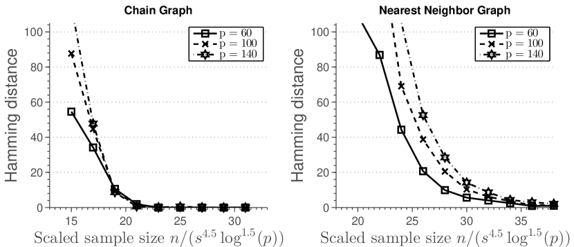
Figure 1: Average hamming distance plotted against the rescaled sample size. Each column represents one simulation setting. Results are averaged over 100 independent runs.

7 Conclusion

In the paper, we focus on sparsistent estimation of the time-varying high-dimensional graph structure in Markov Random Fields from a small size sample. An interesting open direction is estimation of the graph structure from a general time-series, where observations are dependent. In our opinion, the graph structure that changes with time creates the biggest technical difficulties. Incorporating dependent observations would be an easier problem to address, however, the one of great practical importance, since samples in the real data sets are likely to be dependent. Another open direction is to establish necessary conditions, to complement sufficient conditions established here, under which it is possible to estimate a time-varying graph structure. Another research direction may be to use non-convex penalties introduced by Fan and Li (2001) in place of the $\ell_{1}$ penalty. The idea would be to relax the condition imposed in the assumption A2, since it is well known that the SCAD penalties improve performance when the variables are correlated.

Appendix A Large deviation inequalities

In this section we characterize the deviation of elements of the sample Fisher information matrix $\hat{\mathbf{Q}}^{\tau}:=\hat{\mathbf{Q}}_{u}^{\tau}$ at time point $\tau$, defined as

$$\hat{\mathbf{Q}}^{\tau}=\sum_{t}w_{t}^{\tau}\eta(\mathbf{x}^{t};\bm{\theta}_{u}^{\tau})\mathbf{x}_{\backslash u}^{t}\mathbf{x}_{\backslash u}^{t^{\prime}},$$ (A.1)

and the sample covariance matrix $\hat{\bm{\Sigma}}^{\tau}$ from their population versions $\mathbf{Q}^{\tau}$ and $\bm{\Sigma}^{\tau}$. These results are crucial for the proof of the main theorem, where the consistency result depends on the bounds on the difference $\hat{\mathbf{Q}}^{\tau}-\mathbf{Q}^{\tau}$ and $\hat{\bm{\Sigma}}^{\tau}-\bm{\Sigma}^{\tau}$. In the following, we use $C,C^{\prime}$ and $C^{\prime\prime}$ as generic positive constants independent of $(n,p,s)$.

A.1 Sample Fisher information matrix

To bound the deviation between elements of $\hat{\mathbf{Q}}^{\tau}=[\hat{q}_{vv^{\prime}}^{\tau}]$ and $\mathbf{Q}^{\tau}=[q_{vv^{\prime}}^{\tau}]$, $v,v^{\prime}\in V\backslash u$, we will use the following decomposition:

$$|\hat{q}_{vv^{\prime}}^{\tau}-q_{vv^{\prime}}^{\tau}|\ \leq \ |\sum_{t\in\mathcal{T}_{n}}w_{t}^{\tau}\eta(\mathbf{x}^{t};\bm{\theta}_{u}^{\tau})x_{v}^{t}x_{v^{\prime}}^{t}-\sum_{t\in\mathcal{T}_{n}}w_{t}^{\tau}\eta(\mathbf{x}^{t};\bm{\theta}_{u}^{t})x_{v}^{t}x_{v^{\prime}}^{t}|$$ (A.2)

$$+ \ |\sum_{t\in\mathcal{T}_{n}}w_{t}^{\tau}\eta(\mathbf{x}^{t};\bm{\theta}_{u}^{t})x_{v}^{t}x_{v^{\prime}}^{t}-\mathbb{E}[\sum_{t\in\mathcal{T}_{n}}w_{t}^{\tau}\eta(\mathbf{x}^{t};\bm{\theta}_{u}^{t})x_{v}^{t}x_{v^{\prime}}^{t}]|$$

$$+ \ |\mathbb{E}[\sum_{t\in\mathcal{T}_{n}}w_{t}^{\tau}\eta(\mathbf{x}^{t};\bm{\theta}_{u}^{t})x_{v}^{t}x_{v^{\prime}}^{t}]-q_{vv^{\prime}}^{\tau}|.$$

The following lemma gives us bounds on the terms in Eq. (A.2).

Lemma 9.

Assume that the smoothness condition A3 is satisfied and that the kernel function $K(\cdot)$ satisfies A4. Furthermore, assume

$$\max_{t\in[0,1]}|\{v\in\{1,\ldots,p\}\ :\ \theta_{uv}^{t}\neq 0\}|<s,$$

i.e., the number of non-zero elements of the parameter vector is bounded by $s$. There exist constants $C,C^{\prime},C^{\prime\prime}>0$, depending on $M$ and $M_{K}$ only, which are the constants quantifying assumption A3 and A4, respectively , such that for any $\tau\in[0,1]$, we have

$$\max_{v,v^{\prime}}\ |\hat{q}_{vv^{\prime}}^{\tau}-\sum_{t\in\mathcal{T}_{n}}w_{t}^{\tau}\eta(\mathbf{x}^{t};\bm{\theta}_{u}^{t})x_{v}^{t}x_{v^{\prime}}^{t}|\ =\ Csh$$ (A.3)

$$\max_{v,v^{\prime}}\ |\mathbb{E}[\sum_{t\in\mathcal{T}_{n}}w_{t}^{\tau}\eta(\mathbf{x}^{t};\bm{\theta}_{u}^{t})x_{v}^{t}x_{v^{\prime}}^{t}]-q_{vv^{\prime}}^{\tau}|\ =\ C^{\prime}h.$$ (A.4)

Furthermore,

$$|\sum_{t\in\mathcal{T}_{n}}(w_{t}^{\tau}\eta(\mathbf{x}^{t};\bm{\theta}_{u}^{t})x_{v}^{t}x_{v^{\prime}}^{t}-\mathbb{E}[w_{t}^{\tau}\eta(\mathbf{x}^{t};\bm{\theta}_{u}^{t})X_{v}^{t}X_{v^{\prime}}^{t}])|<\epsilon$$ (A.5)

with probability at least $1-2\exp(-C^{\prime\prime}nh\epsilon^{2})$.

Proof.

We start the proof by bounding the difference $|\eta(\mathbf{x};\bm{\theta}_{u}^{t+\delta})-\eta(\mathbf{x};\bm{\theta}_{u}^{t})|$ which will be useful later on. By applying the mean value theorem to $\eta(\mathbf{x};\cdot)$ and the Taylor expansion on $\bm{\theta}_{u}^{t}$ we obtain:

$$|\eta(\mathbf{x};\bm{\theta}_{u}^{t+\delta})-\eta(\mathbf{x};\bm{\theta}_{u}^{t})| =|\sum_{v=1}^{p-1}(\theta_{uv}^{t+\delta}-\theta_{uv}^{t})\eta^{\prime}(\mathbf{x};\bar{\bm{\theta}}_{u}^{(v)})|\qquad\left(\begin{array}[]{c}\bar{\bm{\theta}}_{u}^{(v)}\text{ is a point on the line}\\ \text{between }\bm{\theta}_{u}^{t+\delta}\text{ and }\bm{\theta}_{u}^{t}\end{array}\right)$$

$$\leq\sum_{v=1}^{p-1}|\theta_{uv}^{t+\delta}-\theta_{uv}^{t}|\qquad(\ |\eta^{\prime}(\mathbf{x};\cdot)|\leq 1\ )$$

$$=\sum_{v=1}^{p-1}|\delta\frac{\partial}{\partial t}\theta_{uv}^{t}+\frac{\delta^{2}}{2}\frac{\partial^{2}}{\partial t^{2}}\theta_{uv}^{t}\Big{|}_{t=\beta_{v}}|\qquad\left(\begin{array}[]{c}\beta_{v}\text{ is a point on the line}\\ \text{between }t\text{ and }t+\delta\end{array}\right)$$

Without loss of generality, let $\tau=1$. Using the above equation, and the Riemann integral to approximate the sum, we have

$$|\sum_{t\in\mathcal{T}_{n}}w_{t}^{\tau}\eta(\mathbf{x}^{t};\bm{\theta}_{u}^{\tau})x_{v}^{t}x_{v^{\prime}}^{t}-\sum_{t\in\mathcal{T}_{n}}w_{t}^{\tau}\eta(\mathbf{x}^{t};\bm{\theta}_{u}^{t})x_{v}^{t}x_{v^{\prime}}^{t}|$$

$$\approx|\int\frac{2}{h}K(\frac{z-\tau}{h})[\eta(\mathbf{x}^{z};\bm{\theta}_{u}^{\tau})-\eta(\mathbf{x}^{z};\bm{\theta}_{u}^{z})]x_{v}^{z}x_{v^{\prime}}^{z}dz|$$

$$\leq 2\int_{-\frac{1}{h}}^{0}K(z^{\prime})|\eta(\mathbf{x}^{\tau+z^{\prime}h};\bm{\theta}_{u}^{\tau})-\eta(\mathbf{x}^{\tau+z^{\prime}h};\bm{\theta}_{u}^{\tau+z^{\prime}h})|dz^{\prime}$$

$$\leq 2\int_{-1}^{0}K(z^{\prime})[\sum_{v=1}^{p-1}|z^{\prime}h\frac{\partial}{\partial t}\theta_{uv}^{t}\Big{|}_{t=\tau}+\frac{(z^{\prime}h)^{2}}{2}\frac{\partial^{2}}{\partial t^{2}}\theta_{uv}^{t}\Big{|}_{t=\beta_{v}}|]dz^{\prime}$$

$$\leq Csh,$$

for some constant $C>0$ depending on $M$ from A3 which bounds the derivatives in the equation above, and $M_{K}$ from A4 which bounds the kernel. The last inequality follows from the assumption that the number of non-zero components of the vector $\bm{\theta}_{u}^{t}$ is bounded by $s$.

Next, we prove equation (A.4). Using the Taylor expansion, for any fixed $1\leq v,v^{\prime}\leq p-1$ we have

$$|\mathbb{E} [\sum_{t\in\mathcal{T}_{n}}w_{t}^{\tau}\eta(\mathbf{x}^{t};\bm{\theta}_{u}^{t})x_{v}^{t}x_{v^{\prime}}^{t}]-q_{vv^{\prime}}^{\tau}|$$

$$=|\sum_{t\in\mathcal{T}_{n}}w_{t}^{\tau}(q_{vv^{\prime}}^{t}-q_{vv^{\prime}}^{\tau})|$$

$$=|\sum_{t\in\mathcal{T}_{n}}w_{t}^{\tau}((t-\tau)\frac{\partial}{\partial t}q_{vv^{\prime}}^{t}\Big{|}_{t=\tau}+\frac{(t-\tau)^{2}}{2}\frac{\partial^{2}}{\partial t^{2}}q_{vv^{\prime}}^{t}\Big{|}_{t=\xi}|,$$

where $\xi\in[t,\tau]$. Since $w_{t}^{\tau}=0$ for $|t-\tau|>h$, we have

$$\max_{v,v^{\prime}}|\mathbb{E}[\sum_{t\in\mathcal{T}_{n}}w_{t}^{\tau}\eta(\mathbf{x}^{t};\bm{\theta}_{u}^{t})x_{v}^{t}x_{v^{\prime}}^{t}]-q_{vv^{\prime}}^{\tau}|\leq C^{\prime}h\\$$

for some constant $C>0$ depending on $M$ and $M_{K}$ only.

Finally, we prove equation (A.5). Observe that $w_{t}^{\tau}\eta(\mathbf{x}^{t};\bm{\theta}_{u}^{t})x_{v}^{t}x_{v^{\prime}}^{t}$ are independent and bounded random variables $[-w_{t}^{\tau},w_{t}^{\tau}]$. The equation simply follows from the Hoeffding’s inequality. ∎

Using results of Lemma 9 we can obtain the rate at which the element-wise distance between the true and sample Fisher information matrix decays to zero as a function of the bandwidth parameter $h$ and the size of neighborhood $s$. In the proof of the main theorem, the bandwidth parameter will be chosen so that the bias and variance terms are balanced.

A.2 Sample covariance matrix

The deviation of the elements of the sample covariance matrix is bounded in a similar way as the deviation of elements of the sample Fisher information matrix, given in Lemma 9. Denoting the sample covariance matrix at time point $\tau$ as

$$\hat{\bm{\Sigma}}^{\tau}=\sum_{t}w_{t}^{\tau}\mathbf{x}^{t}\mathbf{x}^{t^{\prime}},$$

and the difference between the elements of $\hat{\bm{\Sigma}}^{\tau}$ and $\bm{\Sigma}^{\tau}$ can be bounded as

$$|\hat{\sigma}_{uv}^{\tau}-\sigma_{uv}^{\tau}| \ =\ |\sum_{t\in\mathcal{T}_{n}}w_{t}^{\tau}x_{u}^{t}x_{v}^{t}-\sigma_{uv}^{\tau}|$$ (A.6)

$$\ \leq\ |\sum_{t\in\mathcal{T}_{n}}w_{t}^{\tau}x_{u}^{t}x_{v}^{t}-\mathbb{E}[\sum_{t\in\mathcal{T}_{n}}w_{t}^{\tau}x_{u}^{t}x_{v}^{t}]|$$

$$\ +\ |\mathbb{E}[\sum_{t\in\mathcal{T}_{n}}w_{t}^{\tau}x_{u}^{t}x_{v}^{t}]-\sigma_{uv}^{\tau}|.$$

The following lemma gives us bounds on the terms in Eq. (A.6).

Lemma 10.

Assume that the smoothness condition A3 is satisfied and that the kernel function $K(\cdot)$ satisfies A4. There are constants $C,C^{\prime}>0$ depending on $M$ and $M_{K}$ only such that for any $\tau\in[0,1]$, we have

$$\max_{u,v}|\mathbb{E}[\sum_{t\in\mathcal{T}_{n}}w_{t}^{\tau}x_{u}^{t}x_{v}^{t}]-\sigma_{uv}^{\tau}|\leq Ch.$$ (A.7)

and

$$|\sum_{t\in\mathcal{T}_{n}}w_{t}^{\tau}x_{u}^{t}x_{v}^{t}-\mathbb{E}[\sum_{t\in\mathcal{T}_{n}}w_{t}^{\tau}x_{u}^{t}x_{v}^{t}]|\leq\epsilon$$ (A.8)

with probability at least $1-2\exp(-C^{\prime}nh\epsilon^{2})$.

Proof.

To obtain the Lemma, we follow the same proof strategy as in the proof of Lemma 9. In particular, Eq. (A.7) is proved in the same way as Eq. (A.4) and Eq. (A.8) in the same way as Eq. (A.5). The details of this derivation are omitted. ∎

Appendix B Technical proofs

In this appendix we provide proofs of lemmas used to prove the main result.

B.1 Proof of Lemma 3

The set of minima $\Theta(\lambda_{n})$ of a convex function is convex. So, for two distinct points of minima, $\bar{\bm{\theta}}_{u}$ and $\tilde{\bm{\theta}_{u}}$, every point on the line connecting two points also belongs to minima, i.e. $\xi\bar{\bm{\theta}_{u}}+(1-\xi)\tilde{\bm{\theta}_{u}}\in\Theta(\lambda_{n})$, for any $\xi\in(0,1)$. Let $\bm{\eta}=\bar{\bm{\theta}}_{u}-\tilde{\bm{\theta}}_{u}$ and now any point on the line can be written as $\tilde{\bm{\theta}}_{u}+\xi\bm{\eta}$. The value of the objective at any point of minima is constant and we have

$$F(\tilde{\bm{\theta}}_{u}+\xi\bm{\eta})=c,\quad\xi\in(0,1),$$

where $c$ is some constant. By taking the derivative with respect to $\xi$ of $F(\tilde{\bm{\theta}}_{u}+\xi\bm{\eta})$ we obtain

$$\sum_{t\in\mathcal{T}_{n}}w_{t}^{\tau} \left[-x_{u}^{t}+\frac{\exp(\langle\tilde{\bm{\theta}}_{u}+\xi\bm{\eta},\mathbf{x}_{\backslash u}^{t}\rangle)-\exp(-\langle\tilde{\bm{\theta}}_{u}+\xi\bm{\eta},\mathbf{x}_{\backslash u}^{t}\rangle)}{\exp(\langle\tilde{\bm{\theta}}_{u}+\xi\bm{\eta},\mathbf{x}_{\backslash u}^{t}\rangle)+\exp(-\langle\tilde{\bm{\theta}}_{u}+\xi\bm{\eta},\mathbf{x}_{\backslash u}^{t}\rangle)}\right]\langle\bm{\eta},\mathbf{x}_{\backslash u}^{t}\rangle$$ (B.1)

$$+\lambda_{n}\sum_{v=1}^{p-1}\eta_{v}\operatorname*{sign}(\tilde{\theta}_{uv}+\xi\eta_{v})=0.$$

On a small neighborhood of $\xi$ the sign of $\tilde{\bm{\theta}}_{u}+\xi\bm{\eta}$ is constant, for each component $v$, since the function $\tilde{\bm{\theta}}_{u}+\xi\bm{\eta}$ is continuous in $\xi$. By taking the derivative with respect to $\xi$ of Eq. (B.1) and noting that the last term is constant on a small neighborhood of $\xi$ we have

$$4\sum_{t\in\mathcal{T}_{n}}w_{t}^{\tau}\langle\bm{\eta},\mathbf{x}_{\backslash u}^{t}\rangle^{2}\frac{\exp(-2\langle\tilde{\bm{\theta}}_{u}+\xi\bm{\eta},\mathbf{x}_{\backslash u}^{t}\rangle)}{\left(1+\exp(-2\langle\tilde{\bm{\theta}}_{u}+\xi\bm{\eta},\mathbf{x}_{\backslash u}^{t}\rangle)\right)^{2}}=0.$$

This implies that $\langle\bm{\eta},\mathbf{x}_{\backslash u}^{t}\rangle=0$ for every $t\in\mathcal{T}_{n}$, which implies that $\langle\mathbf{x}_{\backslash u}^{t},\bar{\bm{\theta}}_{u}\rangle=\langle\mathbf{x}_{\backslash u}^{t},\tilde{\bm{\theta}}_{u}\rangle$, $t\in{\cal T}_{n}$, for any two solutions $\bar{\bm{\theta}}_{u}$ and $\tilde{\bm{\theta}}_{u}$. Since $\bar{\bm{\theta}}_{u}$ and $\tilde{\bm{\theta}}_{u}$ were two arbitrary elements of $\Theta(\lambda_{n})$ we can conclude that $\langle\mathbf{x}_{\backslash u}^{t},\bm{\theta}_{u}\rangle$, $t\in\mathcal{T}_{n}$ is constant for all elements $\bm{\theta}_{u}\in\Theta(\lambda_{n})$.

Next, we need to show that the conclusion from above implies that any two solutions have non-zero elements in the same position. From equation (5.2), it follows that the set of non-zero components of the solution is given by

$$S=\left\{1\leq v\leq p-1\ :\ \left|\sum_{t\in\mathcal{T}_{n}}w_{t}^{\tau}(\nabla\gamma(\bm{\theta}_{u};\mathbf{x}^{t}))_{v}\right|=\lambda\right\}.$$

Using equation (5.3) we have that

$$\sum_{t\in\mathcal{T}_{n}}w_{t}^{\tau}(\nabla\gamma(\bm{\theta}_{u}^{\tau};\mathbf{x}^{t}))_{v}=$$

$$\quad\sum_{t\in\mathcal{T}_{n}}w_{t}^{\tau}(\mathbf{x}_{\backslash u}^{t}\{x_{u}^{t}+1-2\frac{\exp(2x_{u}^{t}\langle\bm{\theta}_{u}^{\tau},\mathbf{x}_{\backslash u}^{t}\rangle)}{\exp(2x_{u}^{t}\langle\bm{\theta}_{u}^{\tau},\mathbf{x}_{\backslash u}^{\tau}\rangle)+1}\})_{v},$$

which is constant across different elements $\bm{\theta}_{u}\in\Theta(\lambda_{n})$, since $\langle\mathbf{x}_{\backslash u}^{t},\bm{\theta}_{u}\rangle$, $t\in{\cal T}_{n}$ is constant for all $\bm{\theta}_{u}\in\Theta(\lambda_{n})$. This implies that the set of non-zero components is the same for all solutions. $\Box$

B.2 Proof of Lemma 4

Under the assumptions given in the Lemma, we can apply the result of Lemma 10. Let $\mathbf{y}\in\mathbb{R}^{s}$ be a unit norm minimal eigenvector of $\hat{\bm{\Sigma}}_{SS}^{\tau}$. We have

$$\Lambda_{\min}(\bm{\Sigma}_{SS}^{\tau}) \ =\ \min_{||\mathbf{x}||_{2}=1}\mathbf{x}^{\prime}\bm{\Sigma}_{SS}^{\tau}\mathbf{x}$$

$$\ =\ \min_{||\mathbf{x}||_{2}=1}\ \{\mathbf{x}^{\prime}\hat{\bm{\Sigma}}_{SS}^{\tau}\mathbf{x}+\mathbf{x}^{\prime}(\bm{\Sigma}_{SS}^{\tau}-\hat{\bm{\Sigma}}_{SS}^{\tau})\mathbf{x}\ \}$$

$$\ \leq\ \mathbf{y}^{\prime}\hat{\bm{\Sigma}}_{SS}^{\tau}\mathbf{y}+\mathbf{y}^{\prime}(\bm{\Sigma}_{SS}^{\tau}-\hat{\bm{\Sigma}}_{SS}^{\tau})\mathbf{y},$$

which implies

$$\Lambda_{\min}(\hat{\bm{\Sigma}}_{SS}^{\tau})\geq D_{\min}-|\!|\!|(\bm{\Sigma}_{SS}^{\tau}-\hat{\bm{\Sigma}}_{SS}^{\tau})|\!|\!|_{{2}}.$$

Let $\bm{\Sigma}^{\tau}=[\sigma_{uv}^{\tau}]$ and $\hat{\bm{\Sigma}}^{\tau}=[\hat{\sigma}_{uv}^{\tau}]$. We have the following bound on the spectral norm

$$|\!|\!|\bm{\Sigma}_{SS}^{\tau}-\hat{\bm{\Sigma}}_{SS}^{\tau}|\!|\!|_{{2}}\leq\left(\sum_{u=1}^{s}\sum_{v=1}^{s}(\hat{\sigma}_{uv}^{\tau}-\sigma_{uv}^{\tau})^{2}\right)^{1/2}\leq\delta,$$

with the probability at least $1-2\exp(-Cnh(\frac{\delta}{s}-C^{\prime}h)^{2}+C^{\prime\prime}\log(s))$, for some fixed constants $C,C^{\prime},C^{\prime\prime}>0$ depending on $M$ and $M_{K}$ only.

Similarly, we have that

$$\Lambda_{\max}(\hat{\bm{\Sigma}}_{SS}^{\tau})\leq D_{\max}+\delta,$$

with probability at least $1-2\exp(-Cnh(\frac{\delta}{s}-C^{\prime}h)^{2}+C^{\prime\prime}\log(s))$, for some fixed constants $C,C^{\prime},C^{\prime\prime}>0$ depending on $M$ and $M_{K}$ only.

From Lemma 3, we know that any two solutions $\bar{\bm{\theta}}_{u},\tilde{\bm{\theta}}_{u}\in\Theta(\lambda_{n})$ of the optimization problem (3.3) have non-zero elements in the same position. So, for any two solutions $\bar{\bm{\theta}}_{u},\tilde{\bm{\theta}}_{u}\in\Theta(\lambda_{n})$, it holds

$$\mathbf{X}_{\backslash u}(\bar{\bm{\theta}}_{u}-\tilde{\bm{\theta}}_{u})=\mathbf{X}_{\backslash u,S}(\bar{\bm{\theta}}_{u}-\tilde{\bm{\theta}}_{u})_{S}+\mathbf{X}_{\backslash u,S^{c}}(\bar{\bm{\theta}}_{u}-\tilde{\bm{\theta}}_{u})_{S^{c}}=\mathbf{X}_{\backslash u,S}(\bar{\bm{\theta}}_{u}-\tilde{\bm{\theta}}_{u})_{S}.$$

Furthermore, from Lemma 3 we know that the two solutions are in the kernel of $\mathbf{X}_{\backslash u,S}$. On the event $\Omega_{01}$, kernel of $\mathbf{X}_{\backslash u,S}$ is $\{0\}$. Thus, the solution is unique on $\Omega_{01}$. $\Box$

B.3 Proof of Lemma 5

We first analyze the probability of the event $\Omega_{02}$. Using the same argument to those in the proof of Lemma 4, we obtain

$$\Lambda_{\min}(\hat{\mathbf{Q}}_{SS}^{\tau})\geq C_{\min}-|\!|\!|\mathbf{Q}_{SS}^{\tau}-\hat{\mathbf{Q}}_{SS}^{\tau}|\!|\!|_{{2}}.$$

Next, using results of Lemma 9, we have the following bound

$$|\!|\!|\mathbf{Q}_{SS}^{\tau}-\hat{\mathbf{Q}}_{SS}^{\tau}|\!|\!|_{{2}}\leq\left(\sum_{u=1}^{s}\sum_{v=1}^{s}(\hat{q}_{uv}^{\tau}-q_{uv}^{\tau})^{2}\right)^{1/2}\leq\delta,$$ (B.2)

with probability at least $1-2\exp(-C\frac{nh\delta^{2}}{s^{2}}+2\log(s))$, for some fixed constants $C,C^{\prime}>0$ depending on $M$ and $M_{K}$ only.

Next, we deal with the event $\Omega_{03}$. We are going to use the following decomposition

$$\hat{\mathbf{Q}}_{S^{c}S}^{\tau}(\hat{\mathbf{Q}}_{SS}^{\tau})^{-1} \ =\ \mathbf{Q}_{S^{c}S}^{\tau}[(\hat{\mathbf{Q}}_{SS}^{\tau})^{-1}-(\mathbf{Q}_{SS}^{\tau})^{-1}]$$

$$\ +\ [\hat{\mathbf{Q}}_{S^{c}S}^{\tau}-\mathbf{Q}_{S^{c}S}^{\tau}](\mathbf{Q}_{SS}^{\tau})^{-1}$$

$$\ +\ [\hat{\mathbf{Q}}_{S^{c}S}^{\tau}-\mathbf{Q}_{S^{c}S}^{\tau}][(\hat{\mathbf{Q}}_{SS}^{\tau})^{-1}-(\mathbf{Q}_{SS}^{\tau})^{-1}]$$

$$\ +\ \mathbf{Q}_{S^{c}S}^{\tau}(\mathbf{Q}_{SS}^{\tau})^{-1}$$

$$\ =\ T_{1}+T_{2}+T_{3}+T_{4}.$$

Under the assumption A2, we have that $|\!|\!|T_{4}|\!|\!|_{{\infty}}\leq 1-\alpha$. The lemma follows if we prove that for all the other terms we have $|\!|\!|\cdot|\!|\!|_{{\infty}}\leq\frac{\alpha}{6}.$ Using the submultiplicative property of the norm, we have for the first term:

$$|\!|\!|T_{1}|\!|\!|_{{\infty}} \ \leq\ |\!|\!|\mathbf{Q}_{S^{c}S}^{\tau}\left(\mathbf{Q}_{SS}^{\tau}\right)^{-1}|\!|\!|_{{\infty}}|\!|\!|\hat{\mathbf{Q}}_{SS}^{\tau}-\mathbf{Q}_{SS}^{\tau}|\!|\!|_{{\infty}}|\!|\!|(\hat{\mathbf{Q}}_{SS}^{\tau})^{-1}|\!|\!|_{{\infty}}$$ (B.3)

$$\ \leq\ (1-\alpha)|\!|\!|\hat{\mathbf{Q}}_{SS}^{\tau}-\mathbf{Q}_{SS}^{\tau}|\!|\!|_{{\infty}}\sqrt{s}|\!|\!|(\hat{\mathbf{Q}}_{SS}^{\tau})^{-1}|\!|\!|_{{2}}.$$

Using Eq. (B.2), we can bound the term $|\!|\!|\left(\hat{\mathbf{Q}}_{SS}^{\tau}\right)^{-1}|\!|\!|_{{2}}\leq C^{\prime\prime}$, for some constant depending on $C_{\min}$ only, with probability at least $1-2\exp(-C\frac{nh}{s}+2\log(s))$, for some fixed constant $C>0$. The bound on the term $|\!|\!|\hat{\mathbf{Q}}_{SS}^{\tau}-\mathbf{Q}_{SS}^{\tau}|\!|\!|_{{\infty}}$ follows from application of Lemma 9. Observe that

$$\mathbb{P}[|\!|\!|\hat{\mathbf{Q}}_{SS}^{\tau}-\mathbf{Q}_{SS}^{\tau}|\!|\!|_{{\infty}}\geq\delta] \ =\ \mathbb{P}[\max_{v\in S}\{\sum_{v^{\prime}\in S}|\hat{q}_{vv^{\prime}}^{\tau}-q_{vv^{\prime}}^{\tau}|\}\geq\delta]$$ (B.4)

$$\ \leq\ 2\exp(-Cnh(\frac{\delta}{s}-C^{\prime}sh)^{2}+2\log(s)),$$

for some fixed constants $C,C^{\prime}>0$. Combining all the elements, we obtain the bound on the first term $|\!|\!|T_{1}|\!|\!|_{{\infty}}\leq\frac{\alpha}{6}$, with probability at least $1-C\exp(C^{\prime}\frac{nh}{s^{3}}+C^{\prime\prime}\log(s))$, for some constants $C,C^{\prime},C^{\prime\prime}>0$.

Next, we analyze the second term. We have that

$$|\!|\!|T_{2}|\!|\!|_{{\infty}} \ \leq\ |\!|\!|\hat{\mathbf{Q}}_{S^{c}S}^{\tau}-\mathbf{Q}_{S^{c}S}^{\tau}|\!|\!|_{{\infty}}\sqrt{s}|\!|\!|\left(\mathbf{Q}_{SS}^{\tau}\right)^{-1}|\!|\!|_{{2}}$$ (B.5)

$$\ \leq\ \frac{\sqrt{s}}{C_{\min}}|\!|\!|\hat{\mathbf{Q}}_{S^{c}S}^{\tau}-\mathbf{Q}_{S^{c}S}^{\tau}|\!|\!|_{{\infty}}.$$

The bound on the term $|\!|\!|\hat{\mathbf{Q}}_{SS}^{\tau}-\mathbf{Q}_{SS}^{\tau}|\!|\!|_{{\infty}}$ follows in the same way as the bound in Eq. (B.4) and we can conclude that $|\!|\!|T_{3}|\!|\!|_{{\infty}}\leq\frac{\alpha}{6}$ with probability at least $1-C\exp(C^{\prime}\frac{nh}{s^{3}}+C^{\prime\prime}\log(p))$, for some constants $C,C^{\prime},C^{\prime\prime}>0$.

Finally, we bound the third term $T_{3}$. We have the following decomposition

$$|\!|\!|[\hat{\mathbf{Q}}_{S^{c}S}^{\tau} -\mathbf{Q}_{S^{c}S}^{\tau}][(\hat{\mathbf{Q}}_{SS}^{\tau})^{-1}-(\mathbf{Q}_{SS}^{\tau})^{-1}]|\!|\!|_{{\infty}}$$

$$\ \leq\ |\!|\!|\hat{\mathbf{Q}}_{S^{c}S}^{\tau}-\mathbf{Q}_{S^{c}S}^{\tau}|\!|\!|_{{\infty}}\sqrt{s}|\!|\!|(\mathbf{Q}_{SS}^{\tau})^{-1}[\mathbf{Q}_{SS}^{\tau}-\hat{\mathbf{Q}}_{SS}^{\tau}](\hat{\mathbf{Q}}_{SS}^{\tau})^{-1}|\!|\!|_{{2}}$$

$$\ \leq\ \frac{\sqrt{s}}{C_{\min}}|\!|\!|\hat{\mathbf{Q}}_{S^{c}S}^{\tau}-\mathbf{Q}_{S^{c}S}^{\tau}|\!|\!|_{{\infty}}|\!|\!|\mathbf{Q}_{SS}^{\tau}-\hat{\mathbf{Q}}_{SS}^{\tau}|\!|\!|_{{2}}|\!|\!|(\hat{\mathbf{Q}}_{SS}^{\tau})^{-1}|\!|\!|_{{2}}.$$

Bounding the remaining terms as in equations (B.5), (B.4) and (B.3), we obtain that $|\!|\!|T_{3}|\!|\!|_{{\infty}}\leq\frac{\alpha}{6}$ with probability at least $1-C\exp(C^{\prime}\frac{nh}{s^{3}}+C^{\prime\prime}\log(p))$.

Bound on the probability of event $\Omega_{03}$ follows from combining the bounds on all terms. $\Box$

B.4 Proof of Lemma 8

To prove this Lemma, we use a technique of Rothman et al. (2008) applied to the problem of consistency of the penalized covariance matrix estimator. Let us define the following function

$$H:\left\{\begin{array}[]{ccl}\mathbb{R}^{p}&\rightarrow&\mathbb{R}\\ \mathbf{D}&\mapsto&F(\bm{\theta}^{\tau}_{u}+\mathbf{D})-F(\bm{\theta}^{\tau}_{u}),\end{array}\right.$$

where the function $F(\cdot)$ is defined in equation (5.1). The function $H(\cdot)$ takes the following form

$$H(\mathbf{D})= \sum_{t\in\mathcal{T}_{n}}w_{t}^{\tau}(\gamma(\bm{\theta}^{\tau}_{u};\mathbf{x}^{t})-\gamma(\bm{\theta}^{\tau}_{u}+\mathbf{D};\mathbf{x}^{t}))$$

$$\ +\ \lambda_{n}(||\bm{\theta}^{\tau}_{u}+\mathbf{D}||_{1}-||\bm{\theta}^{\tau}_{u}||_{1}).$$

Recall the minimizer of (3.3) constructed in the proof of Proposition 6, $\hat{\bm{\theta}}_{u}^{\tau}=(\bar{\bm{\theta}}_{S}^{\prime},0_{S^{c}}^{\prime})^{\prime}$. The minimizer of the function $H(\cdot)$ is $\hat{\mathbf{D}}=\hat{\bm{\theta}}_{u}^{\tau}-\bm{\theta}_{u}^{\tau}$. Function $H(\cdot)$ is convex and $H(0)=0$ by construction. Therefor $H(\hat{\mathbf{D}})\leq 0$. If we show that for some radius $B>0$, and $\mathbf{D}\in\mathbb{R}^{p}$ with $||\mathbf{D}||_{2}=B$ and $\mathbf{D}_{S^{c}}=\mathbf{0}$, we have $H(\mathbf{D})>0$, then we claim that $||\hat{\mathbf{D}}||_{2}\leq B$. This follows from the convexity of $H(\cdot)$.

We proceed to show strict positivity of $H(\cdot)$ on the boundary of the ball with radius $B=K\lambda_{n}\sqrt{s}$, where $K>0$ is a parameter to be chosen wisely later. Let $\mathbf{D}\in\mathbb{R}^{p}$ be an arbitrary vector with $||\mathbf{D}||_{2}=B$ and $\mathbf{D}_{S^{c}}=\mathbf{0}$, then by the Taylor expansion of $\gamma(\cdot;\mathbf{x}^{t})$ we have

$$H(\mathbf{D}) \ =\ -(\sum_{t\in\mathcal{T}_{n}}w_{t}^{\tau}\nabla\gamma(\bm{\theta}^{\tau}_{u};\mathbf{x}^{t}))^{\prime}\mathbf{D}$$ (B.6)

$$\quad\ -\mathbf{D}^{\prime}[\sum_{t\in\mathcal{T}_{n}}w_{t}^{\tau}\eta(\mathbf{x}^{t};\bm{\theta}_{u}^{\tau}+\alpha\mathbf{D})\mathbf{x}_{\backslash u}^{t}\mathbf{x}_{\backslash u}^{t^{\prime}}]\mathbf{D}$$

$$\quad\ +\lambda_{n}(||\bm{\theta}_{u}^{\tau}+\mathbf{D}||_{1}-||\bm{\theta}_{u}^{\tau}||_{1})$$

$$\ =\ (I)+(II)+(III),$$

for some $\alpha\in[0,1]$.

We start from the term $(I)$. Let $\mathbf{e}_{v}\in\mathbb{R}^{p}$ be a unit vector with one at the position $v$ and zeros elsewhere. Then random variables $-\mathbf{e}_{v}^{\prime}\sum_{t\in\mathcal{T}_{n}}w_{t}^{\tau}\nabla\gamma(\bm{\theta}^{\tau}_{u};\mathbf{x}^{t})$ are bounded $[-\frac{C}{nh},\frac{C}{nh}]$ for all $1\leq v\leq p-1$, with constant $C>0$ depending on $M_{K}$ only. Using the Hoeffding inequality and the union bound, we have

$$\max_{1\leq v\leq p-1}|\mathbf{e}_{v}^{\prime}(\sum_{t\in\mathcal{T}_{n}}w_{t}^{\tau}\nabla\gamma(\bm{\theta}^{\tau}_{u};\mathbf{x}^{t})-\mathbb{E}[\sum_{t\in\mathcal{T}_{n}}w_{t}^{\tau}\nabla\gamma(\bm{\theta}^{\tau}_{u};\mathbf{x}^{t})])|\leq\delta,$$

with probability at least $1-2\exp(-Cnh\delta^{2}+\log(p))$, where $C>0$ is a constant depending on $M_{K}$ only. Moreover, denoting

$$p(\bm{\theta}_{u}^{t})=\mathbb{P}_{\bm{\theta}_{u}^{t}}[x_{u}^{t}=1\ |\ \mathbf{x}_{\backslash u}^{t}]$$

to simplify the notation, we have for all $1\leq v\leq p-1$,

$$|\mathbb{E} [\mathbf{e}_{v}^{\prime}\sum_{t\in\mathcal{T}_{n}}w_{t}^{\tau}\nabla\gamma(\bm{\theta}^{\tau}_{u};\mathbf{x}^{t})\ |\ \{\mathbf{x}_{\backslash u}^{t}\}_{t\in\mathcal{T}_{n}}]|$$ (B.7)

$$\ =\ |\mathbb{E}[\sum_{t\in\mathcal{T}_{n}}w_{t}^{\tau}x_{v}^{t}[x_{u}^{t}+1-2p(\bm{\theta}_{u}^{\tau})]\ |\ \{\mathbf{x}_{\backslash u}^{t}\}_{t\in\mathcal{T}_{n}}]|$$

$$\ =\ |2\sum_{t\in\mathcal{T}_{n}}w_{t}^{\tau}x_{v}^{t}[p(\bm{\theta}_{u}^{t})-p(\bm{\theta}_{u}^{\tau})]|$$

$$\ \leq\ 4\int_{-\frac{1}{h}}^{0}K(z)|p(\bm{\theta}_{u}^{\tau+zh})-p(\bm{\theta}_{u}^{\tau})|dz.$$

Next, we apply the mean value theorem on $p(\cdot)$ and the Taylor’s theorem on $\bm{\theta}_{u}^{t}$. Under the assumption A3, we have

$$|p(\bm{\theta}_{u}^{\tau+zh})-p(\bm{\theta}_{u}^{\tau})|$$ (B.8)

$$\qquad\leq\ \sum_{v=1}^{p-1}|\bm{\theta}_{uv}^{\tau+zh}-\theta_{uv}^{\tau}|\qquad(|\ p^{\prime}(\cdot)|\leq 1\ )$$

$$\qquad=\ \sum_{v=1}^{p-1}|zh\frac{\partial}{\partial t}\theta_{uv}^{t}\Big{|}_{t=\tau}+\frac{(zh)^{2}}{2}\frac{\partial^{2}}{\partial t^{2}}\theta_{uv}^{t}\Big{|}_{t=\alpha_{v}}|\qquad(\ \alpha_{v}\in[\tau+zh,\tau]\ )$$

$$\qquad\leq\ Cs|zh+\frac{(zh)^{2}}{2}|,$$

for some $C>0$ depending only on $M$. Combining (B.8) and (B.7) we have that $|\mathbb{E}[\mathbf{e}_{v}^{\prime}\sum_{t\in\mathcal{T}_{n}}w_{t}^{\tau}\nabla\gamma(\bm{\theta}^{\tau}_{u};\mathbf{x}^{t})|\leq Csh$ for all $1\leq v\leq p-1$. Thus, with probability greater than $1-2\exp(-Cnh(\lambda_{n}-sh)^{2}+\log(p))$ for some constant $C>0$ depending only on $M_{K},M$ and $\alpha$, which under the conditions of Theorem 1 goes to 1 exponentially fast, we have

$$\max_{1\leq v\leq p-1}|\mathbf{e}_{v}^{\prime}\sum_{t\in\mathcal{T}_{n}}w_{t}^{\tau}\nabla\gamma(\bm{\theta}^{\tau}_{u};\mathbf{x}^{t})|\leq\frac{\alpha\lambda_{n}}{4(2-\alpha)}<\frac{\lambda_{n}}{4}.$$

On that event, using Hölder’s inequality, we have

$$|(\sum_{t\in\mathcal{T}_{n}}w_{t}^{\tau}\nabla\gamma(\bm{\theta}^{\tau}_{u};\mathbf{x}^{t}))^{\prime}\mathbf{D}| \leq||\mathbf{D}||_{1}\max_{1\leq v\leq p-1}|\mathbf{e}_{v}^{\prime}\sum_{t\in\mathcal{T}_{n}}w_{t}^{\tau}\nabla\gamma(\bm{\theta}^{\tau}_{u};\mathbf{x}^{t})|$$

$$\leq\frac{\lambda_{n}}{4}\sqrt{s}||\mathbf{D}||_{2}\leq(\lambda_{n}\sqrt{s})^{2}\frac{K}{4}.$$

The triangle inequality applied to the term $(III)$ of equation (B.6) yields:

$$\lambda_{n}(||\bm{\theta}_{u}^{\tau}+\mathbf{D}||_{1}-||\bm{\theta}_{u}^{\tau}||_{1}) \geq-\lambda_{n}||\mathbf{D}_{S}||_{1}$$

$$\geq-\lambda_{n}\sqrt{s}||\mathbf{D}_{S}||_{2}\geq-K(\lambda_{n}\sqrt{s})^{2}.$$

Finally, we bound the term $(II)$ of equation (B.6). Observe that since $\mathbf{D}_{S^{c}}=0$, we have

$$\mathbf{D}^{\prime} [\sum_{t\in\mathcal{T}_{n}}w_{t}^{\tau}\eta(\mathbf{x}^{t};\bm{\theta}_{u}^{\tau}+\alpha\mathbf{D})\mathbf{x}_{\backslash u}^{t}\mathbf{x}_{\backslash u}^{t^{\prime}}]\mathbf{D}$$

$$\ =\ \mathbf{D}_{S}^{\prime}[\sum_{t\in\mathcal{T}_{n}}w_{t}^{\tau}\eta(\mathbf{x}^{t};\bm{\theta}_{u}^{\tau}+\alpha\mathbf{D})\mathbf{x}_{S}^{t}\mathbf{x}_{S}^{t^{\prime}}]\mathbf{D}_{S}$$

$$\ \geq\ K^{2}\Lambda_{\min}(\sum_{t\in\mathcal{T}_{n}}w_{t}^{\tau}\eta(\mathbf{x}^{t};\bm{\theta}_{u}^{\tau}+\alpha\mathbf{D})\mathbf{x}_{S}^{t}\mathbf{x}_{S}^{t^{\prime}})$$

Let $g:\mathbb{R}\mapsto\mathbb{R}$ be defined as $g(z)=\frac{4\exp(2z)}{(1+\exp(2z))^{2}}$. Now, $\eta(\mathbf{x};\bm{\theta}_{u})=g(x_{u}\langle\bm{\theta}_{u},\mathbf{x}_{\backslash u}\rangle)$ and we have

$$\Lambda_{\min} (\sum_{t\in\mathcal{T}_{n}}w_{t}^{\tau}\eta(\mathbf{x}^{t};\bm{\theta}_{u}^{\tau}+\alpha\mathbf{D})\mathbf{x}_{S}^{t}\mathbf{x}_{S}^{t^{\prime}})$$

$$\ \geq\ \min_{\alpha\in[0,1]}\Lambda_{\min}(\sum_{t\in\mathcal{T}_{n}}w_{t}\eta(\mathbf{x}^{t};\bm{\theta}_{u}^{\tau}+\alpha\mathbf{D})\mathbf{x}_{S}^{t}\mathbf{x}_{S}^{t^{\prime}})$$

$$\ \geq\ \Lambda_{\min}(\sum_{t\in\mathcal{T}_{n}}w_{t}^{\tau}\eta(\mathbf{x}^{t};\bm{\theta}^{\tau}_{u})\mathbf{x}_{S}^{t}\mathbf{x}_{S}^{t^{\prime}})$$

$$\qquad-\max_{\alpha\in[0,1]}|\!|\!|\sum_{t\in\mathcal{T}_{n}}w_{t}^{\tau}g^{\prime}(x_{u}^{t}\langle\bm{\theta}_{u}^{\tau}+\alpha\mathbf{D},\mathbf{x}_{S}^{t}\rangle)(x_{u}^{t}\mathbf{D}_{S}^{\prime}\mathbf{x}_{S}^{t})\mathbf{x}_{S}^{t}\mathbf{x}_{S}^{t^{\prime}}|\!|\!|_{{2}}$$

$$\ \geq\ C_{\min}-\max_{\alpha\in[0,1]}|\!|\!|\sum_{t\in\mathcal{T}_{n}}w_{t}^{\tau}g^{\prime}(x_{u}^{t}\langle\bm{\theta}_{u}^{\tau}+\alpha\mathbf{D},\mathbf{x}_{S}^{t}\rangle)(x_{u}^{t}\mathbf{D}_{S}^{\prime}\mathbf{x}_{S}^{t})\mathbf{x}_{S}^{t}\mathbf{x}_{S}^{t^{\prime}}|\!|\!|_{{2}}$$

To bound the spectral norm, we observe that for any fixed $\alpha\in[0,1]$ and $y\in\mathbb{R}^{s},||\mathbf{y}||_{2}=1$ we have:

$$\mathbf{y}^{\prime} \{\sum_{t\in\mathcal{T}_{n}}w_{t}^{\tau}g^{\prime}(x_{u}^{t}\langle\bm{\theta}_{u}^{\tau}+\alpha\mathbf{D},\mathbf{x}_{S}^{t}\rangle)(x_{u}^{t}\mathbf{D}_{S}^{\prime}\mathbf{x}_{S}^{t})\mathbf{x}_{S}^{t}\mathbf{x}_{S}^{t^{\prime}}\}\mathbf{y}$$

$$=\sum_{t\in\mathcal{T}_{n}}w_{t}^{\tau}g^{\prime}(x_{u}^{t}\langle\bm{\theta}_{u}^{\tau}+\alpha\mathbf{D},\mathbf{x}_{S}^{t}\rangle)(x_{u}^{t}\mathbf{D}_{S}^{\prime}\mathbf{x}_{S}^{t})(\mathbf{x}_{S}^{t^{\prime}}\mathbf{y})^{2}$$

$$\leq\sum_{t\in\mathcal{T}_{n}}w_{t}^{\tau}|g^{\prime}(x_{u}^{t}\langle\bm{\theta}_{u}^{\tau}+\alpha\mathbf{D},\mathbf{x}_{S}^{t}\rangle)(x_{u}^{t}\mathbf{D}_{S}^{\prime}\mathbf{x}_{S}^{t})|(\mathbf{x}_{S}^{t^{\prime}}\mathbf{y})^{2}$$

$$\leq\sqrt{s}||\mathbf{D}||_{2}|\!|\!|\sum_{t}w_{t}^{\tau}\mathbf{x}_{S}^{t}\mathbf{x}_{S}^{t^{\prime}}|\!|\!|_{{2}}\qquad(\ |g^{\prime}(\cdot)|\leq 1\ )$$

$$\leq D_{\max}K\lambda_{n}s\leq\frac{C_{\min}}{2}.$$

The last inequality follows as long as $\lambda_{n}s\leq\frac{C_{\min}}{2D_{\max}K}$. We have shown that

$$\Lambda_{\min}(\sum_{t\in\mathcal{T}_{n}}w_{t}^{\tau}\eta(\mathbf{x}^{t};\bm{\theta}_{u}^{\tau}+\alpha\mathbf{D})\mathbf{x}_{S}^{t}\mathbf{x}_{S}^{t^{\prime}})\geq\frac{C_{\min}}{2},$$

with high probability.

Putting the bounds on the three terms together, we have

$$H(\mathbf{D})\ \geq\ (\lambda_{n}\sqrt{s})^{2}\left\{-\frac{1}{4}K+\frac{C_{\min}}{2}K^{2}-K\right\},$$

which is strictly positive for $K=\frac{5}{C_{\min}}$. For this choice of $K$, we have that $\lambda_{n}s\leq\frac{C_{\min}^{2}}{10D_{\max}}$, which holds under the conditions of Theorem 1 for $n$ large enough. $\Box$

References

• Ahmed and Xing (2009) A. Ahmed and E. P. Xing. Recovering time-varying networks of dependencies in social and biological studies. Proc. Natl. A. Sci., 106(29):11878–11883, 2009.
• Andrieu et al. (2003) C. Andrieu, M. Davy, and A. Doucet. Efficient particle filtering for jump markov systems. application to time-varying autoregressions. Signal Processing, IEEE Transactions on, 51(7):1762–1770, 2003.
• Banerjee et al. (2008) O. Banerjee, L. El Ghaoui, and A. d’Aspremont. Model selection through sparse maximum likelihood estimation. J. Mach. Learn. Res., 9:485–516, 2008.
• Bresler et al. (2007) G. Bresler, E. Mossel, and A. Sly. Reconstruction of markov random fields from samples: Some easy observations and algorithms. Arxiv, 0712.1402, 2007.
• Cleveland et al. (1991) W. S. Cleveland, E. Grosse, and W. M. Shyu. Local regression models. In J. M. Chambers and T. J. Hastie, editors, Statistical Models in S, pages 309–376, 1991.
• Dobigeon et al. (2007) N. Dobigeon, J.Y. Tourneret, and M. Davy. Joint segmentation of piecewise constant autoregressive processes by using a hierarchical model and a bayesian sampling approach. Signal Processing, IEEE Transactions on, 55(4):1251–1263, 2007.
• Dondelinger et al. (2010) F. Dondelinger, S. Lebre, and D. Husmeier. Heterogeneous continuous dynamic bayesian networks with flexible structure and inter-time segment information sharing. In Proceedings of the 27th International Conference on Machine Learning (ICML-10), 2010.
• Dondelinger et al. (2012) Frank Dondelinger, Sophie Lèbre, and Dirk Husmeier. Non-homogeneous dynamic bayesian networks with bayesian regularization for inferring gene regulatory networks with gradually time-varying structure. Machine Learning, pages 1–40, 2012. ISSN 0885-6125. doi: 10.1007/s10994-012-5311-x.
• Fan and Li (2001) J. Fan and R. Li. Variable selection via nonconcave penalized likelihood and its oracle properties. J. Am. Statist. Ass., 96:1348–1360, 2001.
• Fan et al. (2009) J. Fan, Y. Feng, and Y. Wu. Network exploration via the adaptive LASSO and SCAD penalties. Ann. Appl. Statist., 3(2):521–541, 2009.
• Fearnhead (2006) P. Fearnhead. Exact and efficient bayesian inference for multiple changepoint problems. Statistics and computing, 16(2):203–213, 2006.
• Fox et al. (2011) E. Fox, E.B. Sudderth, M.I. Jordan, and A.S. Willsky. Bayesian nonparametric inference of switching dynamic linear models. Signal Processing, IEEE Transactions on, 59(4):1569–1585, 2011.
• Friedman et al. (2008) J. Friedman, T. Hastie, and R. Tibshirani. Sparse inverse covariance estimation with the graphical lasso. Biostatistics, 9(3):432–441, 2008.
• Friedman et al. (2010) J. Friedman, T. Hastie, and R. Tibshirani. Regularization paths for generalized linear models via coordinate descent, 2010.
• Fujita et al. (2007) A. Fujita, JR Sato, HM Garay-Malpartida, PA Morettin, MC Sogayar, and CE Ferreira. Time-varying modeling of gene expression regulatory networks using the wavelet dynamic vector autoregressive method. Bioinformatics, 23(13):1623–1630, 2007.
• Getoor and Taskar (2007) L. Getoor and B. Taskar. Introduction to Statistical Relational Learning (Adaptive Computation and Machine Learning). The MIT Press, 2007.
• Grzegorczyk and Husmeier (2011a) M. Grzegorczyk and D. Husmeier. Improvements in the reconstruction of time-varying gene regulatory networks: dynamic programming and regularization by information sharing among genes. Bioinformatics, 27(5):693–699, 2011a.
• Grzegorczyk and Husmeier (2012a) M. Grzegorczyk and D. Husmeier. Bayesian regularization of non-homogeneous dynamic bayesian networks by globally coupling interaction parameters. In Proceedings of the 15th International Conference on Artifical Intelligence and Statistics (AISTATS), pages 467–476, 2012a.
• Grzegorczyk and Husmeier (2012b) M. Grzegorczyk and D. Husmeier. A non-homogeneous dynamic bayesian network with sequentially coupled interaction parameters for applications in systems and synthetic biology. Statistical Applications in Genetics and Molecular Biology, 11(4), 2012b.
• Grzegorczyk and Husmeier (2009) Marco Grzegorczyk and Dirk Husmeier. Non-stationary continuous dynamic bayesian networks. In Y. Bengio, D. Schuurmans, J. Lafferty, C. K. I. Williams, and A. Culotta, editors, Advances in Neural Information Processing Systems 22, pages 682–690. 2009.
• Grzegorczyk and Husmeier (2011b) Marco Grzegorczyk and Dirk Husmeier. Non-homogeneous dynamic bayesian networks for continuous data. Mach. Learn., 83(3):355–419, June 2011b. ISSN 0885-6125. doi: 10.1007/s10994-010-5230-7.
• Guo et al. (2010a) J. Guo, E. Levina, G. Michailidis, and J. Zhu. Joint Structure Estimation for Categorical Markov Networks. Unpublished manuscript, 2010a.
• Guo et al. (2010b) J. Guo, E. Levina, G. Michailidis, and J. Zhu. Joint structure estimation for categorical markov networks. Submitted. Available at http://www. stat. lsa. umich. edu/~ elevina, 2010b.
• H. Jiang (2012) F. Liu H. Jiang, A.Lozano. A bayesian markov-switching model for sparse dynamic network estimation. In Proceedings of 2012 SIAM International Conference on Data Mining, 2012.
• Hastie and Tibshirani (1993) T. Hastie and R. Tibshirani. Varying-coefficient models. J. Roy. Statist. Soc. B Met., 55(4):757–796, 1993.
• Husmeier et al. (2010) Dirk Husmeier, Frank Dondelinger, and Sophie Lebre. Inter-time segment information sharing for non-homogeneous dynamic bayesian networks. In J. Lafferty, C. K. I. Williams, J. Shawe-Taylor, R.S. Zemel, and A. Culotta, editors, Advances in Neural Information Processing Systems 23, pages 901–909. 2010.
• Jia and Huan (2010) Yi Jia and Jun Huan. Constructing non-stationary dynamic bayesian networks with a flexible lag choosing mechanism. BMC Bioinformatics, 11(Suppl 6):S27, 2010. ISSN 1471-2105. doi: 10.1186/1471-2105-11-S6-S27.
• Kolar and Xing (2009) M. Kolar and E. P. Xing. Sparsistent Estimation of Time-Varying Discrete Markov Random Fields. ArXiv e-prints, July 2009.
• Kolar and Xing (2010) M. Kolar and E.P. Xing. Estimating Networks With Jumps. Arxiv, 1012.3795, 2010.
• Kolar and Xing (2011) M. Kolar and E.P. Xing. On time varying undirected graphs. In Proceedings of the 14th International Conference on Artificial Intelligence and Statistics, 2011.
• Kolar et al. (2010a) M. Kolar, A. P. Parikh, and E. P. Xing. On sparse nonparametric conditional covariance selection. In ICML ’10: Proc. 27th Ann. Int’l. Conf. Mach. Learn., 2010a.
• Kolar et al. (2010b) M. Kolar, L. Song, A. Ahmed, and E. P. Xing. Estimating Time-Varying networks. Ann. Appl. Statist., 4(1):94–123, 2010b.
• Lebre et al. (2012) S. Lebre, F. Dondelinger, and D. Husmeier. Nonhomogeneous dynamic bayesian networks in systems biology. Methods in Molecular Biology (Clifton, NJ), 802:199–213, 2012.
• Lebre et al. (2010) Sophie Lebre, Jennifer Becq, Frederic Devaux, Michael Stumpf, and Gaelle Lelandais. Statistical inference of the time-varying structure of gene-regulation networks. BMC Systems Biology, 4(1):130, 2010. ISSN 1752-0509. doi: 10.1186/1752-0509-4-130.
• Li and Gui (2006) H. Li and J. Gui. Gradient directed regularization for sparse Gaussian concentration graphs, with applications to inference of genetic networks. Biostatistics, 7(2):302, 2006.
• Meinshausen and Bühlmann (2006) N. Meinshausen and P. Bühlmann. High-dimensional graphs and variable selection with the lasso. Ann. Statist., 34:1436, 2006.
• Peng et al. (2009) J. Peng, P. Wang, N. Zhou, and J. Zhu. Partial correlation estimation by joint sparse regression models. J. Am. Statist. Ass., 104(486):735–746, 2009.
• Punskaya et al. (2002) E. Punskaya, C. Andrieu, A. Doucet, and W.J. Fitzgerald. Bayesian curve fitting using mcmc with applications to signal segmentation. Signal Processing, IEEE Transactions on, 50(3):747–758, 2002.
• Rao et al. (2007) A. Rao, A.O. Hero III, J.D. Engel, et al. Inferring time-varying network topologies from gene expression data. EURASIP Journal on Bioinformatics and Systems Biology, 2007:7–7, 2007.
• Ravikumar et al. (2008) P. Ravikumar, M.J. Wainwright, G. Raskutti, and B. Yu. High-dimensional covariance estimation by minimizing l1-penalized log-determinant divergence. Department of Statistics, UC Berkeley, Tech. Rep, 767, 2008.
• Ravikumar et al. (2010) P. Ravikumar, M. J. Wainwright, and J. D. Lafferty. High-dimensional ising model selection using $\ell_{1}$ regularized logistic regression. Ann. Statist., 38(3):1287–1319, 2010.
• Robinson and Hartemink (2009) Joshua W Robinson and Alexander J Hartemink. Non-stationary dynamic bayesian networks. In D. Koller, D. Schuurmans, Y. Bengio, and L. Bottou, editors, Advances in Neural Information Processing Systems 21, pages 1369–1376. 2009.
• Robinson and Hartemink (2010) J.W. Robinson and A.J. Hartemink. Learning non-stationary dynamic bayesian networks. The Journal of Machine Learning Research, 11:3647–3680, 2010.
• Rothman et al. (2008) A.J. Rothman, P.J. Bickel, E. Levina, and J. Zhu. Sparse permutation invariant covariance estimation. Electron. J. Statist., 2:494–515, 2008.
• Siracusa and Fisher (2009) M.R. Siracusa and JW Fisher. Tractable bayesian inference of time-series dependence structure. In Proceedings of AISTATS, 2009.
• Song et al. (2009a) L. Song, M. Kolar, and E. P. Xing. Keller: Estimating time-evolving interactions between genes. In Proc. 16th Int’l. Conf. Intell. Syst. Molec. Bio., 2009a.
• Song et al. (2009b) Le Song, Mladen Kolar, and Eric Xing. Time-varying dynamic bayesian networks. In Y. Bengio, D. Schuurmans, J. Lafferty, C. K. I. Williams, and A. Culotta, editors, Advances in Neural Information Processing Systems 22, pages 1732–1740. 2009b.
• Talih and Hengartner (2005) M. Talih and N. Hengartner. Structural learning with time-varying components: tracking the cross-section of financial time series. Journal of the Royal Statistical Society: Series B (Statistical Methodology), 67(3):321–341, 2005.
• Vogel and Fried (2010) D. Vogel and R. Fried. On robust gaussian graphical modelling. In L. Devroye et al. (Eds.), editor, Recent Developments in Applied Probability and Statistics, pages 155–182. Berlin, Heidelberg: Springer-Verlag, 2010.
• Wainwright and Jordan (2008) M. J. Wainwright and M. I. Jordan. Graphical models, exponential families, and variational inference. Found. Trends Mach. Learn., 1(1-2):1–305, 2008.
• Wang et al. (2009) P. Wang, D. L. Chao, and L. Hsu. Learning networks from high dimensional binary data: An application to genomic instability data. Arxiv, 0908.3882, 2009.
• Wang et al. (2011) Z. Wang, E.E. Kuruoglu, X. Yang, Y. Xu, and T.S. Huang. Time varying dynamic bayesian network for nonstationary events modeling and online inference. Signal Processing, IEEE Transactions on, 59(4):1553–1568, 2011.
• Xuan and Murphy (2007) Xiang Xuan and Kevin Murphy. Modeling changing dependency structure in multivariate time series. In Proceedings of the 24th international conference on Machine learning, ICML ’07, pages 1055–1062, New York, NY, USA, 2007. ACM. ISBN 978-1-59593-793-3. doi: 10.1145/1273496.1273629.
• Yin et al. (2010) J. Yin, Z. Geng, R. Li, and H. Wang. Nonparametric covariance model. Statist. Sin., 20:469–479, 2010.
• Yoshida et al. (2005) Ryo Yoshida, Seiya Imoto, and Tomoyuki Higuchi. Estimating time-dependent gene networks from time series microarray data by dynamic linear models with markov switching. In Proceedings of the 2005 IEEE Computational Systems Bioinformatics Conference, CSB ’05, pages 289–298, Washington, DC, USA, 2005. IEEE Computer Society. ISBN 0-7695-2344-7. doi: 10.1109/CSB.2005.32.
• Yuan and Lin (2007) M. Yuan and Y. Lin. Model selection and estimation in the gaussian graphical model. Biometrika, 94(1):19–35, 2007.
• Zhou et al. (2008) S. Zhou, J. Lafferty, and L. Wasserman. Time varying undirected graphs. In Rocco A. Servedio and Tong Zhang, editors, COLT, pages 455–466. Omnipress, 2008.