Dynamical state reduction in an EPR experiment

Abstract

A model is developed to describe state reduction in an EPR experiment as a continuous, relativistically-invariant, dynamical process. The system under consideration consists of two entangled isospin particles each of which undergo isospin measurements at spacelike separated locations. The equations of motion take the form of stochastic differential equations. These equations are solved explicitly in terms of random variables with a priori known probability distribution in the physical probability measure. In the course of solving these equations a correspondence is made between the state reduction process and the problem of classical nonlinear filtering. It is shown that the solution is covariant, violates Bell inequalities, and does not permit superluminal signaling. It is demonstrated that the model is not governed by the Free Will Theorem and it is argued that the claims of Conway and Kochen, that there can be no relativistic theory providing a mechanism for state reduction, are false.

I Introduction

The motivation for attempting to formulate a dynamical description of state reduction pearlorig0 ; pearlorig ; gisin ; ghir3 ; dios2 ; ghir2 stems from the inherent problems of quantum measurement. In standard quantum theory the state reduction postulate is a necessary supplement to the Schrödinger dynamics in order that we can realise definite measurement outcomes from the potentiality of the initial state vector. The problem with this picture is that the pragmatic application of these two different laws of evolution is left to the judgment of the physicist rather than being fixed by exact mathematical formulation. Our experience in the use of quantum theory tells us that the state reduction postulate should not be applied to a microscopic system consisting of a few elementary particles until it interacts with a macroscopic object such as a measuring device. This works perfectly well in practice for current experimental technologies, but as we begin to explore systems on intermediate scales it is not clear whether state reduction should be assumed or not. A solution of the problem of measurement thus requires that we somehow set a fundamental scale to demarcate micro and macro effects within the dynamical framework.

The formulation of an empirical model, objectively describing the dynamics of the state reduction process is a direct approach to achieving this aim. The basic requirements we have for such a model can be characterised as follows Bass ; Pear2 :

• Measurements involving macroscopic instruments should have definite outcomes.

• The statistical connections between measurement outcomes and the state vector prior to measurement should be preserved.

• The model should be consistent with known experimental results.

The task of meeting these objectives in a relativistic context has met with technical difficulties related to renormalization pear3 ; ghir1 ; adle ; Pear ; Nicr ; tumul ; pearshape ; me . These issues derive from the quantum field theoretic nature of relativistic systems. In this paper we will attempt to sidestep this problem by considering a simplified quantum system with a finite-dimensional Hilbert space free from the problem of divergences. Our aim is to elucidate the dynamical process of state reduction in a relativistic context.

We will consider a model describing the famous experiment devised by Einstein, Podolski, and Rosen (EPR) EPR . The experiment involves two elementary particles in an entangled state and separated by a spacelike interval. The original purpose of EPR was to argue that quantum mechanics is fundamentally incomplete as a theory. In order to do this they made a locality assumption stating that the two particles are not able to instantaneously influence each other at a distance. Theoretical and experimental advances Bell ; aspe have since demonstrated the remarkable conclusion that the assumption of locality is incorrect. Entangled quantum systems can indeed transmit instantaneous influence at a distance when a measurement is performed. Although this fact negates the EPR argument, instead it poses questions for our understanding of quantum measurement. In particular, the notion of instantaneous influence due to state reduction during measurement seems to sit uncomfortably with the theory of relativity.

A formal relativistically-covariant description of the state reduction associated with measurement has been given by Aharanov and Albert aa3 . They show that for a consistent description of the measurement process, the state evolution cannot take the form of a function on spacetime. The proposed solution is that state evolution should be described by a functional on the set of spacelike hypersurfaces as conceived by Tomonaga and Schwinger. This sets the scene for understanding how to formulate a fully dynamical and relativistic description of the state reduction process.

Relativistic dynamical reduction models have been critically investigated from the perspective of the analysis of Aharanov and Albert by Ghirardi Ghir4 . There, the conceptual features of these models are discussed and shown to lead to a coherent picture. It is the intention of this work to extend the analysis of Ghirardi by constructing an explicit model of continuous state evolution. Our model, which is described in detail in section II, is designed to highlight the peculiar nonlocal features. In sections III and IV we derive closed-form solutions to the stochastic equations of motion. The value of this is that it enables us to examine the nonlocal character of the stochastic noise processes. In section V we apply the method of Brody and Hughston Dorj ; Dorj2 to demonstrate that the equations describing the dynamical state reduction can be viewed as a description of a classical filtering problem. In section VI we generalise our model to consider an experiment where the experimenter can freely choose which measurement to perform on the individual particle from an incompatible set of possible measurements. This leads us to a discussion of the so-called Free Will Theorem fw1 ; fw2 ; Bass2 ; fwt2 ; fw3 of Conway and Kochen in section VII. We use our findings to argue that the axiomatic assumptions of the Free Will Theorem are too restrictive and that the conclusions of the theorem cannot be applied to dynamical models of state reduction.

II The model

We consider two particles denoted ${\it 1}$ and ${\it 2}$, each described by an internal isospin-$\textstyle\frac{1}{2}$ degree of freedom. The choice of an isospin system avoids complication encountered when dealing with conventional spin in a covariant formulation. The initial isospin state of the two particles is defined in spacetime on an initial spacelike hypersurface $\sigma_{i}$ as the isospin singlet state

$$|\psi(\sigma_{i})\rangle=\mbox{$\textstyle\frac{1}{\sqrt{2}}$}\left\{|+\mbox{$\textstyle\frac{1}{2}$};-\mbox{$\textstyle\frac{1}{2}$}\rangle-|-\mbox{$\textstyle\frac{1}{2}$};+\mbox{$\textstyle\frac{1}{2}$}\rangle\right\}.$$ (1)

The isospin states for each particle are represented with respect to a fixed axis in isospin space.

The particle trajectories in spacetime are assumed to behave classically. The two particles move in separate directions away from some specific location where they have been prepared. Each particle path eventually intersects with the path of an isospin measuring device. This leads to a localised interaction which we assume takes place in some finite region of spacetime. We assume that the classical trajectories of the particles and measuring devices, and the finite regions of interaction are determined. Further we assume that the two measurement regions are completely spacelike separated in the sense that every point in each region is spacelike separated from every point in the other region. We denote the two measurement regions by $R_{\it 1}$ and $R_{\it 2}$ (see figure 1).

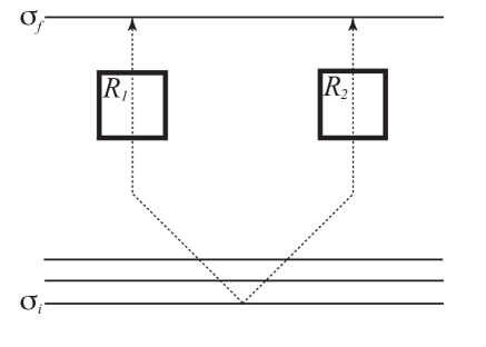
Figure 1: The diagram represents an experiment to measure the states of two entangled particles. The dashed lines are the (classical) particle trajectories where particle 1 moves to the left and particle 2 moves to the right. The vertical represents a timelike direction whilst the horizontal represents a spacelike direction. We suppose that within the spacetime region $R_{\it 1}$, a measurement is performed on particle ${\it 1}$. Similarly within the spacetime region $R_{\it 2}$ (spacelike separated from $R_{\it 1}$), a measurement is performed on particle ${\it 2}$. The initial state is defined on the spacelike hypersurface $\sigma_{i}$. The state advances as described by the Tomonaga picture through a sequence of spacelike surfaces defining a foliation of spacetime.

In order to describe the state evolution we use the Tomonaga picture Tomo ; Schw . Standard unitary dynamics are described in this picture by the Tomonaga equation,

$$\frac{\delta|\psi(\sigma)\rangle}{\delta\sigma(x)}=-iH_{\rm int}(x)|\psi(\sigma)\rangle,$$ (2)

where $H_{\rm int}$ is the interaction Hamiltonian. Given two spacelike hypersurfaces $\sigma$ and $\sigma^{\prime}$ differing only by some small spacetime volume $\Delta\omega$ about some spacetime point $x$, the functional derivative is defined by

$$\frac{\delta|\psi(\sigma)\rangle}{\delta\sigma(x)}=\lim_{\sigma^{\prime}\rightarrow\sigma}\frac{|\psi(\sigma^{\prime})\rangle-|\psi(\sigma)\rangle}{\Delta\omega}.$$ (3)

The operator $H_{\rm int}$ must be a scalar in order that equation (2) has Lorentz invariant form. We must also have $[H_{\rm int}(x),H_{\rm int}(x^{\prime})]=0$ for spacelike separated $x$ and $x^{\prime}$ reflecting the fact that there is no temporal ordering between spacelike separated points.

In differential form equation (2) can be written

$$\mbox{$\rm d$}_{x}|\psi(\sigma)\rangle=-iH_{\rm int}(x)\mbox{$\rm d$}\omega|\psi(\sigma)\rangle$$ (4)

where $\mbox{$\rm d$}_{x}|\psi(\sigma)\rangle$ represents the infinitesimally small change in the state as the hypersurface $\sigma$ is deformed in a timelike direction at point $x$.

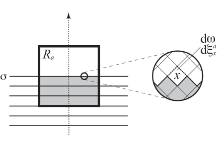
Figure 2: The diagram represents a sequence of spacelike hypersurfaces advancing through the spacetime region $R_{a}$. The gray shading within $R_{a}$ corresponds to the spacetime volume $\omega_{\sigma}^{a}$. The detail shows a small spacetime region within $R_{a}$ where the surface $\sigma$ advances through a spacetime cell at point $x$. Associated with the cell at point $x$ is the incremental spacetime volume $\mbox{$\rm d$}\omega$ and the incremental Brownian variable $\mbox{$\rm d$}\xi_{x}^{a}$.

We specify a probability space $(\Omega,{\cal F},\mathbb{Q})$ along with a filtration ${\cal F}^{\xi}_{\sigma}$ of ${\cal F}$ generated by a two-dimensional $\mathbb{Q}$-Brownian motion $\{\xi^{\it 1}_{\sigma},\xi^{\it 2}_{\sigma}\}$. For each interaction region $R_{a}$ ($a={\it 1},{\it 2}$) the spacelike hypersurfaces $\{\sigma\}$ characterise the time evolution for each component of the Brownian motion. Given a foliation of spacetime, we define a “time difference” between any two surfaces as the spacetime volume enclosed by the surfaces within the region $R_{a}$. Consider the set $(\sigma_{i},\sigma)$ of all spacetime points between the two spacelike surfaces $\sigma_{i}$ and $\sigma$, and consider the intersection of this set with the interaction region $(\sigma_{i},\sigma)\cap R_{a}$. We denote the spacetime volume of $(\sigma_{i},\sigma)\cap R_{a}$ by $\omega_{\sigma}^{a}$ (see the gray shaded region in figure 2). The two volumes $\omega_{\sigma}^{\it 1}$ and $\omega_{\sigma}^{\it 2}$ correspond to two different time parameters for the two component Brownian motions. This definition ensures that time increases monotonically as the future surface ${\sigma}$ advances. The parameterization is covariant and has the convenience of only being relevant during the predefined measurement events. We define an infinitesimal increment of the Brownian motion $\mbox{$\rm d$}\xi^{a}_{x}$ (relating to two spacelike hypersurfaces which differ only by an infinitesimal spacetime volume $\mbox{$\rm d$}\omega$ at point $x$) by the following:

$$\mbox{$\rm d$}\xi^{a}_{x} = 0,\;\;\text{for $x\notin R_{a}$};$$

$$\mathbb{E}^{\mathbb{Q}}[\mbox{$\rm d$}\xi^{a}_{x}|{\cal F}_{\sigma}^{\xi}] = 0,\;\;\text{for $x$ to the future of $\sigma$};$$

$$\mbox{$\rm d$}\xi^{a}_{x}\mbox{$\rm d$}\xi^{b}_{y} = \delta^{ab}\delta_{xy}\mbox{$\rm d$}\omega,\;\;\text{for $x\in R_{a}$, $y\in R_{b}$},$$ (5)

where $\mathbb{E}^{\mathbb{Q}}[\cdot|{\cal F}_{\sigma}^{\xi}]$ denotes conditional expectation in $\mathbb{Q}$. We attribute $\mbox{$\rm d$}\xi^{a}_{x}$ to the spacetime point $x$ independent of any spacelike surface on which $x$ may lie. The two-dimensional Brownian motion is given by the sum of all infinitesimal Brownian increments belonging to the set of points $(\sigma_{i},\sigma)\cap R_{a}$,

$$\xi_{\sigma}^{a}=\int_{\sigma_{i}}^{\sigma}\mbox{$\rm d$}\xi^{a}_{x},$$ (6)

so that an increment of the process can be written

$$\xi_{\sigma^{\prime}}^{a}-\xi_{\sigma}^{a}=\int_{\sigma}^{\sigma^{\prime}}\mbox{$\rm d$}\xi^{a}_{x},$$ (7)

where $\sigma^{\prime}$ is to the future of $\sigma$. These increments are independent and have mean zero and variance $\omega_{\sigma^{\prime}}^{a}-\omega_{\sigma}^{a}$ as can easily be demonstrated by comparison with the conventional time parameterization of Brownian motion.

The state reduction process which occurs as the isospin state is measured can now be described by extension of the Tomonaga equation (4) to include a stochastic term. We define our evolution by

$$\mbox{$\rm d$}_{x}|\psi(\sigma)\rangle = \left\{2\lambda S_{\it 1}\mbox{$\rm d$}\xi^{\it 1}_{x}-\mbox{$\textstyle\frac{1}{2}$}\lambda^{2}\mbox{$\rm d$}\omega\right\}|\psi(\sigma)\rangle\;\;\text{for}\;\;x\in R_{\it 1},$$

$$\mbox{$\rm d$}_{x}|\psi(\sigma)\rangle = \left\{2\lambda S_{\it 2}\mbox{$\rm d$}\xi^{\it 2}_{x}-\mbox{$\textstyle\frac{1}{2}$}\lambda^{2}\mbox{$\rm d$}\omega\right\}|\psi(\sigma)\rangle\;\;\text{for}\;\;x\in R_{\it 2},$$

$$\mbox{$\rm d$}_{x}|\psi(\sigma)\rangle = 0\;\;{\rm otherwise}.$$ (8)

The operators $S_{a}$ are isospin operators for each particle with the properties

$$S_{\it 1}|\pm\mbox{$\textstyle\frac{1}{2}$};\;\cdot\;\rangle=\pm\mbox{$\textstyle\frac{1}{2}$}|\pm\mbox{$\textstyle\frac{1}{2}$};\;\cdot\;\rangle\;\;,\;\;S_{\it 2}|\;\cdot\;;\pm\mbox{$\textstyle\frac{1}{2}$}\rangle=\pm\mbox{$\textstyle\frac{1}{2}$}|\;\cdot\;;\pm\mbox{$\textstyle\frac{1}{2}$}\rangle;$$ (9)

the parameter $\lambda$ is a coupling parameter. The model explicitly describes an experiment to measure the isospin state of each particle in the given fixed isospin direction (the case of a general isospin measurement direction will be considered below). The form of equations (8) can be roughly understood by considering an incremental stage in the evolution where $\mbox{$\rm d$}\xi^{a}_{\sigma}$ is either positive or negative. For example, if $\mbox{$\rm d$}\xi^{\it 1}_{\sigma}$ is positive then the stochastic term on the right side of the first equation in (8) will augment the $+\mbox{$\textstyle\frac{1}{2}$}$ state for particle ${\it 1}$ whilst degrading the $-\mbox{$\textstyle\frac{1}{2}$}$ state for particle ${\it 1}$. The opposite happens if $\mbox{$\rm d$}\xi^{\it 1}_{\sigma}$ is negative. Eventually after a certain period of evolution one of the two eigenstates will dominate. This is analogous to the famous problem of the gambler’s ruin.

The drift terms on the right side of equations (8) ensure that the state norm is a positive martingale

$$\mbox{$\rm d$}_{x}\langle\psi(\sigma)|\psi(\sigma)\rangle = 4\lambda\langle\psi(\sigma)|S_{\it 1}|\psi(\sigma)\rangle\mbox{$\rm d$}\xi_{x}^{\it 1}\;\;\text{for}\;\;x\in R_{\it 1},$$

$$\mbox{$\rm d$}_{x}\langle\psi(\sigma)|\psi(\sigma)\rangle = 4\lambda\langle\psi(\sigma)|S_{\it 2}|\psi(\sigma)\rangle\mbox{$\rm d$}\xi_{x}^{\it 2}\;\;\text{for}\;\;x\in R_{\it 2}.$$ (10)

We can then define a physical measure $\mathbb{P}$ equivalent to $\mathbb{Q}$ according to

$$\mathbb{E}^{\mathbb{P}}[\cdot|{\cal F}_{\sigma}^{\xi}]=\frac{\mathbb{E}^{\mathbb{Q}}[\langle\psi(\sigma_{f})|\psi(\sigma_{f})\rangle\cdot|{\cal F}_{\sigma}^{\xi}]}{\mathbb{E}^{\mathbb{Q}}[\langle\psi(\sigma_{f})|\psi(\sigma_{f})\rangle|{\cal F}_{\sigma}^{\xi}]}=\frac{\mathbb{E}^{\mathbb{Q}}[\langle\psi(\sigma_{f})|\psi(\sigma_{f})\rangle\cdot|{\cal F}_{\sigma}^{\xi}]}{\langle\psi(\sigma)|\psi(\sigma)\rangle},$$ (11)

with $\sigma_{f}$ the final surface of the state evolution we are considering. This change of measure ensures that physical outcomes are weighted according to the Born rule, meeting the second bullet-pointed criterion for dynamical state reduction stated in the introduction. Note that the processes $\xi_{\sigma}^{a}$ satisfy a modified distribution under the $\mathbb{P}$-measure.

Our model can be interpreted as an effective model describing the interaction of the two particles with macroscopic measuring devices in regions $R_{\it 1}$ and $R_{\it 2}$. In more detail we would expect the particle states to become correlated with different states of the measuring devices. The state reduction dynamics would be expected to have a negligible effect on the individual spin particles, however, the effect would be rapid for a macroscopic superposition of measuring device states. Collapse of the spin particle would then occur indirectly as a result of collapse of the macro state. In our model we have assumed that the particle states undergo a direct collapse dynamics. This allows us to ignore the fine details of the interaction between spin particles and measuring devices.

By designating spacetime regions where collapse of the isospin state occurs we avoid the issue of setting a scale distinguishing micro and macro behaviour. Our main interest here is to understand the dynamical process of state reduction for an entangled quantum system in a relativistic setting.

III Solution in terms of $\mathbb{Q}$-Brownian motion

Working in the $\mathbb{Q}$-measure where $\xi_{\sigma}^{a}$ is a Brownian process we find the following solution for the unnormalised state evolution:

$$|\psi(\sigma)\rangle=\mbox{$\textstyle\frac{1}{\sqrt{2}}$}\left\{e^{\lambda\xi_{\sigma}^{\it 1}-\lambda^{2}\omega_{\sigma}^{\it 1}}e^{-\lambda\xi_{\sigma}^{\it 2}-\lambda^{2}\omega_{\sigma}^{\it 2}}|+\mbox{$\textstyle\frac{1}{2}$};-\mbox{$\textstyle\frac{1}{2}$}\rangle-e^{-\lambda\xi_{\sigma}^{\it 1}-\lambda^{2}\omega_{\sigma}^{\it 1}}e^{\lambda\xi_{\sigma}^{\it 2}-\lambda^{2}\omega_{\sigma}^{\it 2}}|-\mbox{$\textstyle\frac{1}{2}$};+\mbox{$\textstyle\frac{1}{2}$}\rangle\right\}.$$ (12)

This can easily be checked with the use of (5), (6), and (8). The state norm is given by

$$\langle\psi(\sigma)|\psi(\sigma)\rangle=\mbox{$\textstyle\frac{1}{2}$}\left\{e^{2\lambda\xi_{\sigma}^{\it 1}-2\lambda^{2}\omega_{\sigma}^{\it 1}}e^{-2\lambda\xi_{\sigma}^{\it 2}-2\lambda^{2}\omega_{\sigma}^{\it 2}}+e^{-2\lambda\xi_{\sigma}^{\it 1}-2\lambda^{2}\omega_{\sigma}^{\it 1}}e^{2\lambda\xi_{\sigma}^{\it 2}-2\lambda^{2}\omega_{\sigma}^{\it 2}}\right\}.$$ (13)

We note that although equation (12) is a solution to (8), it cannot be considered as a solution to the model since it completely disregards the important role played by the physical measure $\mathbb{P}$. Equation (12) enables us to generate sample outcomes, however, the physical probability density at a given outcome can only be determined afterwards with reference to the state norm (a likely outcome in $\mathbb{Q}$ may be highly unlikely in $\mathbb{P}$).

We define the characteristic function associated with $\xi_{\sigma}^{\it 1}$ and $\xi_{\sigma}^{\it 2}$ in the $\mathbb{P}$-measure as

$$\Phi_{\sigma}^{\xi}(t_{\it 1},t_{\it 2}) = \mathbb{E}^{\mathbb{P}}\left[e^{it_{\it 1}\xi_{\sigma}^{\it 1}}e^{it_{\it 2}\xi_{\sigma}^{\it 2}}|{\cal F}_{\sigma_{i}}^{\xi}\right]$$ (14)

$$= \mathbb{E}^{\mathbb{Q}}\left[\langle\psi(\sigma)|\psi(\sigma)\rangle e^{it_{\it 1}\xi_{\sigma}^{\it 1}}e^{it_{\it 2}\xi_{\sigma}^{\it 2}}|{\cal F}_{\sigma_{i}}^{\xi}\right],$$ (15)

where we have used equation (11) and the fact that the initial state has unit norm. Noting that $\xi_{\sigma}^{\it 1}$ and $\xi_{\sigma}^{\it 2}$ are independent in the $\mathbb{Q}$-measure we can determine the expectation using equation (13) to find

$$\Phi_{\sigma}^{\xi}(t_{\it 1},t_{2})=\mbox{$\textstyle\frac{1}{2}$}\left\{e^{2i\lambda t_{\it 1}\omega_{\sigma}^{\it 1}-\frac{1}{2}t_{\it 1}^{2}\omega_{\sigma}^{\it 1}}e^{-2i\lambda t_{\it 2}\omega_{\sigma}^{\it 2}-\frac{1}{2}t_{\it 2}^{2}\omega_{\sigma}^{\it 2}}+e^{-2i\lambda t_{\it 1}\omega_{\sigma}^{\it 1}-\frac{1}{2}t_{\it 1}^{2}\omega_{\sigma}^{\it 1}}e^{2i\lambda t_{\it 2}\omega_{\sigma}^{\it 2}-\frac{1}{2}t_{\it 2}^{2}\omega_{\sigma}^{\it 2}}\right\}.$$ (16)

The characteristic function allows us to immediately demonstrate that spacelike separated processes $\xi_{\sigma}^{1}$ and $\xi_{\sigma}^{2}$ are correlated under the physical measure $\mathbb{P}$:

$$\mathbb{E}^{\mathbb{P}}\left[\xi_{\sigma}^{a}|{\cal F}_{\sigma_{i}}^{\xi}\right] = -i\frac{\mbox{$\rm d$}}{\mbox{$\rm d$}t_{a}}\left.\left[\Phi_{\sigma}^{\xi}(t_{\it 1},t_{\it 2})\right]\right|_{t_{\it 1}=t_{\it 2}=0}=0,$$

$$\mathbb{E}^{\mathbb{P}}\left[\xi_{\sigma}^{\it 1}\xi_{\sigma}^{\it 2}|{\cal F}_{\sigma_{i}}^{\xi}\right] = -\frac{\mbox{$\rm d$}^{2}}{\mbox{$\rm d$}t_{\it 1}\mbox{$\rm d$}t_{\it 2}}\left.\left[\Phi_{\sigma}^{\xi}(t_{\it 1},t_{\it 2})\right]\right|_{t_{\it 1}=t_{\it 2}=0}=-4\lambda^{2}\omega^{\it 1}_{\sigma}\omega^{\it 2}_{\sigma}.$$ (17)

The stochastic information at one wing of the apparatus is not independent of the stochastic information at the other wing. We might expect this since the results of the two measurements that the information dictate are correlated.

Before demonstrating the state reducing properties of this model, we first show in the next section how to express the solution (12) directly in terms of a $\mathbb{P}$-Brownian motion. This will allow us to generate physical sample solutions.

IV Solution in terms of $\mathbb{P}$-Brownian motion

Let the probability space $(\Omega,{\cal F},\mathbb{P})$ be given and let ${\cal G}_{\sigma}$ be a filtration of ${\cal F}$ such that independent $\mathbb{P}$-Brownian motions $B_{\sigma}^{a}$ ($a={\it 1},{\it 2}$) are specified together with random variables $s_{a}$ (independent of $B_{\sigma}^{a}$). The Brownian motions $B_{\sigma}^{a}$ are defined under the $\mathbb{P}$-measure in the same way in which Brownian motions $\xi_{\sigma}^{a}$ are defined under $\mathbb{Q}$-measure by equations (5) and (6). The probability distribution for the random variables $s_{a}$ are given by

$$\mathbb{P}\left(s_{\it 1}=+\mbox{$\textstyle\frac{1}{2}$},s_{\it 2}=-\mbox{$\textstyle\frac{1}{2}$}\right) = \mbox{$\textstyle\frac{1}{2}$},$$

$$\mathbb{P}\left(s_{\it 1}=-\mbox{$\textstyle\frac{1}{2}$},s_{\it 2}=+\mbox{$\textstyle\frac{1}{2}$}\right) = \mbox{$\textstyle\frac{1}{2}$}.$$ (18)

We assume that $s_{a}$ are ${\cal G}_{\sigma_{i}}$-measurable.

Now define the random processes (c.f. Dorj2 )

$$\xi_{\sigma}^{\it 1} = 4\lambda s_{\it 1}\omega_{\sigma}^{\it 1}+B_{\sigma}^{\it 1},$$

$$\xi_{\sigma}^{\it 2} = 4\lambda s_{\it 2}\omega_{\sigma}^{\it 2}+B_{\sigma}^{\it 2}.$$ (19)

Our aim is to show that these processes, defined under the $\mathbb{P}$-measure, can be identified as the $\mathbb{Q}$-Brownian processes $\xi_{\sigma}^{a}$ involved in the equations of motion for the state (8). In order to do this we must show that their characteristic function under the $\mathbb{P}$-measure is identical to that found for the $\mathbb{Q}$-Brownian processes, as given by equation (16).

Again let ${\cal F}_{\sigma}^{\xi}$ denote the filtration generated by $\{\xi_{\sigma}^{\it 1},\xi_{\sigma}^{\it 2}\}$. The use of ${\cal F}_{\sigma}^{\xi}$ ensures that we have no more or less information than is given by the processes $\{\xi_{\sigma}^{\it 1},\xi_{\sigma}^{\it 2}\}$ as in the original presentation of the model in section II. Neither $s_{a}$ nor $B_{\sigma}^{a}$ are ${\cal F}_{\sigma}^{\xi}$-measurable. The only information we have regarding the realisation of these variables is $\{\xi_{\sigma}^{\it 1},\xi_{\sigma}^{\it 2}\}$.

The characteristic function for $\xi_{\sigma}^{\it 1}$ and $\xi_{\sigma}^{\it 2}$ is given by equation (14),

$$\Phi_{\sigma}^{\xi}(t_{\it 1},t_{\it 2})=\mathbb{E}^{\mathbb{P}}\left[e^{it_{\it 1}\xi_{\sigma}^{\it 1}}e^{it_{\it 2}\xi_{\sigma}^{\it 2}}|{\cal F}_{\sigma_{i}}^{\xi}\right],$$

but now we write

$$\Phi_{\sigma}^{\xi}(t_{\it 1},t_{\it 2}) = \mbox{$\textstyle\frac{1}{2}$}\mathbb{E}^{\mathbb{P}}\left[\left.e^{it_{\it 1}(4\lambda s_{\it 1}\omega_{\sigma}^{\it 1}+B_{\sigma}^{\it 1})}e^{it_{\it 2}(4\lambda s_{\it 2}\omega_{\sigma}^{\it 2}+B_{\sigma}^{\it 2})}\right|{\cal F}_{\sigma_{i}}^{\xi};s_{\it 1}=+\mbox{$\textstyle\frac{1}{2}$},s_{\it 2}=-\mbox{$\textstyle\frac{1}{2}$}\right]$$ (20)

$$+\mbox{$\textstyle\frac{1}{2}$}\mathbb{E}^{\mathbb{P}}\left[\left.e^{it_{\it 1}(4\lambda s_{\it 1}\omega_{\sigma}^{\it 1}+B_{\sigma}^{\it 1})}e^{it_{\it 2}(4\lambda s_{\it 2}\omega_{\sigma}^{\it 2}+B_{\sigma}^{\it 2})}\right|{\cal F}_{\sigma_{i}}^{\xi};s_{\it 1}=-\mbox{$\textstyle\frac{1}{2}$},s_{\it 2}=+\mbox{$\textstyle\frac{1}{2}$}\right].$$

Noting that $B_{\sigma}^{\it 1}$ and $B_{\sigma}^{\it 2}$ are independent we can work directly in the $\mathbb{P}$-measure to confirm that the characteristic function is once more given by equation (16). This demonstrates that the processes defined by equation (19) can indeed be identified as $\mathbb{Q}$-Brownian motions $\xi_{\sigma}^{a}$.

We are now in a position to express the solution to equations (8) and (11) in terms of the $\mathbb{P}$-Brownian motions $B_{\sigma}^{a}$, and the random variables $s_{a}$. This is summarised in the following subsection. The fact that the solution is expressed in terms of variables with an a priori known probability distribution in the physical measure is to be contrasted with the solution in terms of $\mathbb{Q}$-Brownian motion where physical probabilities can only be determined a posteriori with knowledge of the state norm.

IV.1 Summary of solution

The solution to the equations of motion (8) is given by the unnormalised state

$$|\psi(\sigma)\rangle=\mbox{$\textstyle\frac{1}{\sqrt{2}}$}\left\{e^{\lambda\xi_{\sigma}^{\it 1}-\lambda^{2}\omega_{\sigma}^{\it 1}}e^{-\lambda\xi_{\sigma}^{\it 2}-\lambda^{2}\omega_{\sigma}^{\it 2}}|+\mbox{$\textstyle\frac{1}{2}$};-\mbox{$\textstyle\frac{1}{2}$}\rangle-e^{-\lambda\xi_{\sigma}^{\it 1}-\lambda^{2}\omega_{\sigma}^{\it 1}}e^{\lambda\xi_{\sigma}^{\it 2}-\lambda^{2}\omega_{\sigma}^{\it 2}}|-\mbox{$\textstyle\frac{1}{2}$};+\mbox{$\textstyle\frac{1}{2}$}\rangle\right\}.$$ (21)

(This is the same solution in terms of $\xi_{\sigma}^{a}$ as presented in equation (12), however, we now treat $\xi_{\sigma}^{a}$, not as a $\mathbb{Q}$-Brownian motion, but as an information process defined in terms of variables with known $\mathbb{P}$-distributions.) The random variables $\xi_{\sigma}^{a}$ are given by

$$\xi_{\sigma}^{\it 1} = 4\lambda s_{\it 1}\omega_{\sigma}^{\it 1}+B_{\sigma}^{\it 1},$$

$$\xi_{\sigma}^{\it 2} = 4\lambda s_{\it 2}\omega_{\sigma}^{\it 2}+B_{\sigma}^{\it 2}.$$ (22)

The stochastic processes $B_{\sigma}^{\it 1}$ and $B_{\sigma}^{\it 2}$ are independent $\mathbb{P}$-Brownian motions. The random variables $s_{a}$ take values $s_{\it 1}=+1/2,s_{\it 2}=-1/2$ with probability $1/2$ and $s_{\it 1}=-1/2,s_{\it 2}=+1/2$ with probability $1/2$. Brownian motions $B_{\sigma}^{a}$ and random variables $s^{a}$ are independent. Only the processes $\xi_{\sigma}^{a}$ are measurable.

This solution is as relativistically invariant as a description of state reduction can be. We expect the state to depend on the spacelike surface $\sigma$ we choose to query. The dependence on $\sigma$ results in equation (21) from the spacetime volume variables $\omega_{\sigma}^{a}$ and the random variables $B_{\sigma}^{a}$. We note that neither of these variables depends on the chosen foliation of spacetime. For example, the distribution of $B_{\sigma}^{a}$ is characterized by the spacetime volume $\omega_{\sigma}^{a}$ which in turn is determined only by the surface $\sigma$. A foliation dependence would be undesirable as it would indicate a preferred frame in the model. The fact that there is no foliation dependence indicates also that the choice $\sigma$ has no prior physical significance.

IV.2 State reduction

In this subsection we explicitly demonstrate how the solution outlined above exhibits state reduction to a state of well-defined isospin. Consider the isospin operators $S_{a}$. The conditional expectation of $S_{a}$ for the state $|\psi(\sigma)\rangle$ is given by

$$\langle S_{a}\rangle_{\sigma}=\frac{\langle\psi(\sigma)|S_{a}|\psi(\sigma)\rangle}{\langle\psi(\sigma)|\psi(\sigma)\rangle}.$$ (23)

From equation (21) we find choosing, for example, $a={\it 1}$,

$$\langle S_{\it 1}\rangle_{\sigma}=\frac{\mbox{$\textstyle\frac{1}{2}$}e^{2\lambda\xi_{\sigma}^{\it 1}-2\lambda^{2}\omega_{\sigma}^{\it 1}}e^{-2\lambda\xi_{\sigma}^{\it 2}-2\lambda^{2}\omega_{\sigma}^{\it 2}}-\mbox{$\textstyle\frac{1}{2}$}e^{-2\lambda\xi_{\sigma}^{\it 1}-2\lambda^{2}\omega_{\sigma}^{\it 1}}e^{2\lambda\xi_{\sigma}^{\it 2}-2\lambda^{2}\omega_{\sigma}^{\it 2}}}{e^{2\lambda\xi_{\sigma}^{\it 1}-2\lambda^{2}\omega_{\sigma}^{\it 1}}e^{-2\lambda\xi_{\sigma}^{\it 2}-2\lambda^{2}\omega_{\sigma}^{\it 2}}+e^{-2\lambda\xi_{\sigma}^{\it 1}-2\lambda^{2}\omega_{\sigma}^{\it 1}}e^{2\lambda\xi_{\sigma}^{\it 2}-2\lambda^{2}\omega_{\sigma}^{\it 2}}}.$$ (24)

Now suppose we condition on the event $s_{\it 1}=+1/2,s_{\it 2}=-1/2$. We find

$$\langle S_{\it 1}\rangle_{\sigma} = \frac{\mbox{$\textstyle\frac{1}{2}$}e^{2\lambda B_{\sigma}^{\it 1}+2\lambda^{2}\omega_{\sigma}^{\it 1}}e^{-2\lambda B_{\sigma}^{\it 2}+2\lambda^{2}\omega_{\sigma}^{\it 2}}-\mbox{$\textstyle\frac{1}{2}$}e^{-2\lambda B_{\sigma}^{\it 1}-6\lambda^{2}\omega_{\sigma}^{\it 1}}e^{2\lambda B_{\sigma}^{\it 2}-6\lambda^{2}\omega_{\sigma}^{\it 2}}}{e^{2\lambda B_{\sigma}^{\it 1}+2\lambda^{2}\omega_{\sigma}^{\it 1}}e^{-2\lambda B_{\sigma}^{\it 2}+2\lambda^{2}\omega_{\sigma}^{\it 2}}+e^{-2\lambda B_{\sigma}^{\it 1}-6\lambda^{2}\omega_{\sigma}^{\it 1}}e^{2\lambda B_{\sigma}^{\it 2}-6\lambda^{2}\omega_{\sigma}^{\it 2}}}$$ (25)

$$= \frac{\mbox{$\textstyle\frac{1}{2}$}-\mbox{$\textstyle\frac{1}{2}$}e^{-4\lambda B_{\sigma}^{\it 1}-8\lambda^{2}\omega_{\sigma}^{\it 1}}e^{4\lambda B_{\sigma}^{\it 2}-8\lambda^{2}\omega_{\sigma}^{\it 2}}}{1+e^{-4\lambda B_{\sigma}^{\it 1}-8\lambda^{2}\omega_{\sigma}^{\it 1}}e^{4\lambda B_{\sigma}^{\it 2}-8\lambda^{2}\omega_{\sigma}^{\it 2}}}.$$

Next we use the result that

$$\lim_{\omega_{\sigma}\rightarrow\infty}\mathbb{P}\left(e^{\pm 4\lambda B_{\sigma}-8\lambda^{2}\omega_{\sigma}}>0\right)=0,$$ (26)

to deduce that $\langle S_{\it 1}\rangle_{\sigma}\rightarrow 1/2$ as $\omega_{\sigma}^{\it 1}\rightarrow\infty$ or $\omega_{\sigma}^{\it 2}\rightarrow\infty$. These volumes increase in size as the surface $\sigma$ passes the spacetime regions $R_{\it 1}$ and $R_{\it 2}$ respectively. Since these regions are of finite size, $\omega_{\sigma}^{\it 1}$ and $\omega_{\sigma}^{\it 1}$ can only attain fixed maximal values. We assume that these maximal values are sufficiently large that the limit of equation (26) is approached with high precision. Note that the rate at which this limit is approached can be controlled by the choice of coupling parameter $\lambda$.

A similar analysis leads to the conclusion that $\langle S_{\it 2}\rangle_{\sigma}\rightarrow-1/2$. Conversely, if we were to condition on the event $s_{\it 1}=-1/2,s_{\it 2}=+1/2$, we would find $\langle S_{\it 1}\rangle_{\sigma}\rightarrow-1/2$ and $\langle S_{\it 2}\rangle_{\sigma}\rightarrow 1/2$. We observe that the unmeasurable random variable $s_{a}$ dictates the outcome of the experiment. Only the processes $\xi_{\sigma}^{a}$ are known to the state; the Brownian processes $B_{\sigma}^{a}$ act as noise terms obscuring the values $s_{a}$.

IV.3 Probabilities for reduction

Here we demonstrate that the stochastic probabilities for outcomes are those predicted by the quantum state prior to the measurement event. For example, we define the $+\mbox{$\textstyle\frac{1}{2}$}$ state projection operator on particle ${\it 1}$ by

$$P_{\it 1}^{+}|+\mbox{$\textstyle\frac{1}{2}$};\;\cdot\;\rangle=|+\mbox{$\textstyle\frac{1}{2}$};\;\cdot\;\rangle\;\;;\;\;P_{\it 1}^{+}|-\mbox{$\textstyle\frac{1}{2}$};\;\cdot\;\rangle=0,$$ (27)

and the conditional expectation of this operator for the state $|\psi(\sigma)\rangle$ by

$$\langle P_{\it 1}^{+}\rangle_{\sigma}=\frac{\langle\psi(\sigma)|P_{\it 1}^{+}|\psi(\sigma)\rangle}{\langle\psi(\sigma)|\psi(\sigma)\rangle}.$$ (28)

In order to calculate the unconditional expectation of $\langle P_{\it 1}^{+}\rangle_{\sigma}$ it turns out to be simpler to work in the $\mathbb{Q}$-measure. We proceed as follows:

$$\mathbb{E}^{\mathbb{P}}[\langle P_{\it 1}^{+}\rangle_{\sigma}|{\cal F}_{\sigma_{i}}^{\xi}] = \mathbb{E}^{\mathbb{Q}}[\langle\psi(\sigma)|\psi(\sigma)\rangle\langle P_{\it 1}^{+}\rangle_{\sigma}|{\cal F}_{\sigma_{i}}^{\xi}]$$ (29)

$$= \mathbb{E}^{\mathbb{Q}}[\langle\psi(\sigma)|P_{\it 1}^{+}|\psi(\sigma)\rangle|{\cal F}_{\sigma_{i}}^{\xi}]$$

$$= \mathbb{E}^{\mathbb{Q}}\left.\left[\mbox{$\textstyle\frac{1}{2}$}e^{2\lambda\xi_{\sigma}^{\it 1}-2\lambda^{2}\omega_{\sigma}^{\it 1}}e^{-2\lambda\xi_{\sigma}^{\it 2}-2\lambda^{2}\omega_{\sigma}^{\it 2}}\right|{\cal F}_{\sigma_{i}}^{\xi}\right]=\mbox{$\textstyle\frac{1}{2}$}.$$

From the previous subsection we know that as $\omega_{\sigma}^{a}\rightarrow\infty$ then the state of each particle tends towards a definite isospin state and consequently the conditional expectation of $P_{\it 1}^{+}$ tends to either 0 or 1. This means that as $\omega_{\sigma}^{a}\rightarrow\infty$ we have

$$\mathbb{E}^{\mathbb{P}}[\langle P_{\it 1}^{+}\rangle_{\sigma}|{\cal F}_{\sigma_{i}}^{\xi}]=\mathbb{E}^{\mathbb{P}}\left.\left[\mathds{1}_{\left\{\langle S_{\it 1}\rangle_{\sigma}=\mbox{$\textstyle\frac{1}{2}$}\right\}}\right|{\cal F}_{\sigma_{i}}^{\xi}\right]=\mathbb{P}\left.\left(\langle S_{\it 1}\rangle_{\sigma}=\mbox{$\textstyle\frac{1}{2}$}\right|{\cal F}_{\sigma_{i}}^{\xi}\right),$$ (30)

where $\mathds{1}_{\{E\}}$ takes the value 1 if the event $E$ is true, and 0 otherwise. From equation (29) we can now write

$$\mathbb{P}\left.\left(\langle S_{\it 1}\rangle_{\sigma}=\mbox{$\textstyle\frac{1}{2}$}\right|{\cal F}_{\sigma_{i}}^{\xi}\right)=\mbox{$\textstyle\frac{1}{2}$}=\langle P_{\it 1}^{+}\rangle_{\sigma_{i}}.$$ (31)

This tells us that as the dynamics lead to a definite state for each particle then the stochastic probability of a given outcome matches the initial quantum probability. The same is true of other projection operators as can easily be shown.

V Interpretation in terms of nonlinear filtering

In this section we use the method of Brody and Hughston Dorj ; Dorj2 to demonstrate that the problem under consideration can be interpreted as a classical nonlinear filtering problem. The method was originally applied to solve an energy-based state diffusion equation.

From section IV.2 we understand that the ${\cal F}_{\sigma}^{\xi}$-unmeasurable random variables $s_{a}$ represent the true outcomes for the isospin eigenvalues of each particle after the measurement process. Only information in the form $\xi_{\sigma}^{a}=4\lambda s_{a}\omega_{\sigma}^{a}+B_{\sigma}^{a}$ is accessible to the state where the realised value of $s_{a}$ is masked by the ${\cal F}_{\sigma}^{\xi}$-unmeasurable noise processes $B_{\sigma}^{a}$.

Suppose we attempt to address the problem of finding $s_{a}$ directly, that is, given $\{\xi_{\sigma}^{a}\}$ what is the best estimate we can make for $s_{a}$. This is a classical nonlinear filtering problem. It is straightforward to show that the best estimate for the value of $s_{a}$ is given by the conditional expectation

$$\widehat{s_{a}}_{\sigma}=\mathbb{E}^{\mathbb{P}}\left[\left.s_{a}\right|{\cal F}_{\sigma}^{\xi}\right].$$ (32)

The aim is now to identify $\widehat{s_{a}}_{\sigma}$ with the quantum expectation processes $\langle S_{a}\rangle_{\sigma}$.

We first show that $\xi_{\sigma}^{a}$ are Markov processes. To do this we show that

$$\mathbb{P}\left(\left.\xi_{\sigma}^{a}<y\right|\xi_{\sigma_{1}}^{\it 1},\xi_{\sigma_{2}}^{\it 1},\cdots,\xi_{\sigma_{k}}^{\it 1};\xi_{\sigma_{1}}^{\it 2},\xi_{\sigma_{2}}^{\it 2},\cdots,\xi_{\sigma_{k}}^{\it 2}\right)=\mathbb{P}\left(\left.\xi_{\sigma}^{a}<y\right|\xi_{\sigma_{1}}^{\it 1};\xi_{\sigma_{1}}^{\it 2}\right)$$ (33)

where $\{\sigma,\sigma_{1},\sigma_{2},\cdots,\sigma_{k}\}$ is a sequence of spacelike surfaces belonging to some spacetime foliation such that

$$\omega_{\sigma}^{\it 1} \geq \omega_{\sigma_{1}}^{\it 1}\geq\omega_{\sigma_{2}}^{\it 1}\geq\cdots\geq\omega_{\sigma_{k}}^{\it 1}>0,$$

$$\omega_{\sigma}^{\it 2} \geq \omega_{\sigma_{1}}^{\it 2}\geq\omega_{\sigma_{2}}^{\it 2}\geq\cdots\geq\omega_{\sigma_{k}}^{\it 2}>0.$$ (34)

The proof of equation (33) is more or less identical to that given by Brody and Hughston Dorj . We use the fact that $\mathbb{E}^{\mathbb{P}}[B_{\sigma^{\prime}}^{b}B_{\sigma^{\prime\prime}}^{b}]=\omega_{\sigma^{\prime}}^{b}$, where $\omega_{\sigma^{\prime\prime}}^{b}\geq\omega_{\sigma^{\prime}}^{b}$ for $b={\it 1},{\it 2}$. Then for $\omega_{\sigma}^{b}\geq\omega_{\sigma_{1}}^{b}\geq\omega_{\sigma_{2}}^{b}>0$ we have that

$$B_{\sigma}^{b}{\rm\;\;and\;\;}\frac{B_{\sigma_{1}}^{b}}{\omega_{\sigma_{1}}^{b}}-\frac{B_{\sigma_{2}}^{b}}{\omega_{\sigma_{2}}^{b}}{\rm\;\;are\;\;independent}.$$ (35)

Furthermore,

$$\frac{B_{\sigma_{1}}^{b}}{\omega_{\sigma_{1}}^{b}}-\frac{B_{\sigma_{2}}^{b}}{\omega_{\sigma_{2}}^{b}}=\frac{\xi_{\sigma_{1}}^{b}}{\omega_{\sigma_{1}}^{b}}-\frac{\xi_{\sigma_{2}}^{b}}{\omega_{\sigma_{2}}^{b}},$$ (36)

from which it follows that

$$\mathbb{P}\left(\left.\xi_{\sigma}^{a}<y\right|\xi_{\sigma_{1}}^{\it 1},\xi_{\sigma_{2}}^{\it 1},\xi_{\sigma_{3}}^{\it 1},\cdots;\xi_{\sigma_{1}}^{\it 2},\xi_{\sigma_{2}}^{\it 2},\xi_{\sigma_{3}}^{\it 2},\cdots\right)$$ (37)

$$= \mathbb{P}\left(\left.\xi_{\sigma}^{a}<y\right|\xi_{\sigma_{1}}^{\it 1},\frac{\xi_{\sigma_{1}}^{\it 1}}{\omega_{\sigma_{1}}^{\it 1}}-\frac{\xi_{\sigma_{2}}^{\it 1}}{\omega_{\sigma_{2}}^{\it 1}},\frac{\xi_{\sigma_{2}}^{\it 1}}{\omega_{\sigma_{2}}^{\it 1}}-\frac{\xi_{\sigma_{3}}^{\it 1}}{\omega_{\sigma_{3}}^{\it 1}},\cdots;\xi_{\sigma_{1}}^{\it 2},\frac{\xi_{\sigma_{1}}^{\it 2}}{\omega_{\sigma_{1}}^{\it 2}}-\frac{\xi_{\sigma_{2}}^{\it 2}}{\omega_{\sigma_{2}}^{\it 2}},\frac{\xi_{\sigma_{2}}^{\it 2}}{\omega_{\sigma_{2}}^{\it 2}}-\frac{\xi_{\sigma_{3}}^{\it 2}}{\omega_{\sigma_{3}}^{\it 2}},\cdots\right)$$

$$= \mathbb{P}\left(\left.\xi_{\sigma}^{a}<y\right|\xi_{\sigma_{1}}^{\it 1},\frac{B_{\sigma_{1}}^{\it 1}}{\omega_{\sigma_{1}}^{\it 1}}-\frac{B_{\sigma_{2}}^{\it 1}}{\omega_{\sigma_{2}}^{\it 1}},\frac{B_{\sigma_{2}}^{\it 1}}{\omega_{\sigma_{2}}^{\it 1}}-\frac{B_{\sigma_{3}}^{\it 1}}{\omega_{\sigma_{3}}^{\it 1}},\cdots;\xi_{\sigma_{1}}^{\it 2},\frac{B_{\sigma_{1}}^{\it 2}}{\omega_{\sigma_{1}}^{\it 2}}-\frac{B_{\sigma_{2}}^{\it 2}}{\omega_{\sigma_{2}}^{\it 2}},\frac{B_{\sigma_{2}}^{\it 2}}{\omega_{\sigma_{2}}^{\it 2}}-\frac{B_{\sigma_{3}}^{\it 2}}{\omega_{\sigma_{3}}^{\it 2}},\cdots\right).$$

Now from (35) we have that $\xi_{\sigma}^{a}$, $\xi_{\sigma_{1}}^{\it 1}$, and $\xi_{\sigma_{1}}^{\it 2}$ are each independent of $B_{\sigma_{1}}^{\it 1}/\omega_{\sigma_{1}}^{\it 1}-B_{\sigma_{2}}^{\it 1}/\omega_{\sigma_{2}}^{\it 1}$, $B_{\sigma_{2}}^{\it 1}/\omega_{\sigma_{2}}^{\it 1}-B_{\sigma_{3}}^{\it 1}/\omega_{\sigma_{3}}^{\it 1}$, etc. Equation (33) follows. The same argument shows that

$$\mathbb{P}\left(\left.B_{\sigma}^{a}<y\right|\xi_{\sigma_{1}}^{\it 1},\xi_{\sigma_{2}}^{\it 1},\cdots,\xi_{\sigma_{k}}^{\it 1};\xi_{\sigma_{1}}^{\it 2},\xi_{\sigma_{2}}^{\it 2},\cdots,\xi_{\sigma_{k}}^{\it 2}\right)=\mathbb{P}\left(\left.B_{\sigma}^{a}<y\right|\xi_{\sigma_{1}}^{\it 1};\xi_{\sigma_{1}}^{\it 2}\right),$$ (38)

and therefore

$$\mathbb{P}\left(\left.s_{a}=\pm\mbox{$\textstyle\frac{1}{2}$}\right|{\cal F}_{\sigma}^{\xi}\right)=\mathbb{P}\left(\left.s_{a}=\pm\mbox{$\textstyle\frac{1}{2}$}\right|\xi_{\sigma}^{\it 1};\xi_{\sigma}^{\it 2}\right).$$ (39)

Next we use a version of Bayes formula to calculate this conditional probability

$$\mathbb{P}\left(\left.s_{\it 1}=\pm\mbox{$\textstyle\frac{1}{2}$},s_{\it 2}=\mp\mbox{$\textstyle\frac{1}{2}$}\right|\xi_{\sigma}^{\it 1};\xi_{\sigma}^{\it 2}\right)=\frac{\mathbb{P}\left(s_{\it 1}=\pm\mbox{$\textstyle\frac{1}{2}$},s_{\it 2}=\mp\mbox{$\textstyle\frac{1}{2}$}\right)\rho\left(\left.\xi_{\sigma}^{\it 1};\xi_{\sigma}^{\it 2}\right|s_{\it 1}=\pm\mbox{$\textstyle\frac{1}{2}$},s_{\it 2}=\mp\mbox{$\textstyle\frac{1}{2}$}\right)}{\rho\left(\xi_{\sigma}^{\it 1};\xi_{\sigma}^{\it 2}\right)}.$$ (40)

The density function for the random variables $(\xi_{\sigma}^{\it 1};\xi_{\sigma}^{\it 2})$ conditional on $s_{a}$ is Gaussian (since $B_{\sigma}^{a}$ is a Brownian motion under $\mathbb{P}$) and is given by

$$\rho\left(\left.\xi_{\sigma}^{\it 1};\xi_{\sigma}^{\it 2}\right|s_{\it 1}=\pm\mbox{$\textstyle\frac{1}{2}$},s_{\it 2}=\mp\mbox{$\textstyle\frac{1}{2}$}\right) \propto e^{-\frac{1}{2\omega_{\sigma}^{\it 1}}\left(\xi_{\sigma}^{\it 1}\mp 2\lambda\omega_{\sigma}^{\it 1}\right)^{2}}e^{-\frac{1}{2\omega_{\sigma}^{\it 2}}\left(\xi_{\sigma}^{\it 2}\pm 2\lambda\omega_{\sigma}^{\it 2}\right)^{2}}.$$ (41)

We also have that

$$\rho\left(\xi_{\sigma}^{\it 1};\xi_{\sigma}^{\it 2}\right)=\mbox{$\textstyle\frac{1}{2}$}\rho\left(\left.\xi_{\sigma}^{\it 1},\xi_{\sigma}^{\it 2}\right|s_{\it 1}=+\mbox{$\textstyle\frac{1}{2}$},s_{\it 2}=-\mbox{$\textstyle\frac{1}{2}$}\right)+\mbox{$\textstyle\frac{1}{2}$}\rho\left(\left.\xi_{\sigma}^{\it 1},\xi_{\sigma}^{\it 2}\right|s_{\it 1}=-\mbox{$\textstyle\frac{1}{2}$},s_{\it 2}=+\mbox{$\textstyle\frac{1}{2}$}\right).$$ (42)

We are now in a position to calculate the conditional expectation $\widehat{s_{a}}_{\sigma}$ given by equation (32). For example, choosing $a={\it 1}$ we have

$$\widehat{s_{\it 1}}_{\sigma}=\mathbb{E}^{\mathbb{P}}\left[\left.s_{\it 1}\right|{\cal F}_{\sigma}^{\xi}\right] = \mbox{$\textstyle\frac{1}{2}$}\mathbb{P}\left(\left.s_{\it 1}=+\mbox{$\textstyle\frac{1}{2}$},s_{\it 2}=-\mbox{$\textstyle\frac{1}{2}$}\right|\xi_{\sigma}^{\it 1};\xi_{\sigma}^{\it 2}\right)-\mbox{$\textstyle\frac{1}{2}$}\mathbb{P}\left(\left.s_{\it 1}=-\mbox{$\textstyle\frac{1}{2}$},s_{\it 2}=+\mbox{$\textstyle\frac{1}{2}$}\right|\xi_{\sigma}^{\it 1};\xi_{\sigma}^{\it 2}\right)$$ (43)

$$= \frac{\mbox{$\textstyle\frac{1}{2}$}e^{2\lambda\xi_{\sigma}^{\it 1}}e^{-2\lambda\xi_{\sigma}^{\it 2}}-\mbox{$\textstyle\frac{1}{2}$}e^{-2\lambda\xi_{\sigma}^{\it 1}}e^{2\lambda\xi_{\sigma}^{\it 2}}}{e^{2\lambda\xi_{\sigma}^{\it 1}}e^{-2\lambda\xi_{\sigma}^{\it 2}}+e^{-2\lambda\xi_{\sigma}^{\it 1}}e^{2\lambda\xi_{\sigma}^{\it 2}}}.$$

This is the same expression as that given for $\langle S_{\it 1}\rangle_{\sigma}$ in equation (24). This demonstrates that the conditional expectation $\widehat{s_{\it 1}}_{\sigma}$, which represents our best estimate for the random variable $s_{\it 1}$ given only information from the filtration ${\cal F}^{\xi}_{\sigma}$, corresponds to the quantum expectation of the operator $S_{\it 1}$, conditional on the same information. It is remarkable that the complexity of the stochastic quantum formalism corresponds to a such a conceptually intuitive classical analogue.

VI Bell test experiments

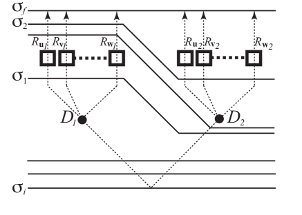
Figure 3: A Bell test experiment for two entangled isospin particles. The dashed lines are the (classical) particle trajectories where particle 1 moves initially to the left and particle 2 moves initially to the right. The vertical represents a timelike direction whilst the horizontal represents a spacelike direction. At $D_{\it 1}$ a device is used to deflect particle 1 towards one of several measuring devices each set up to perform an isospin measurement for a different orientation in isospin space. Spacetime regions $R_{{\bf u}_{\it 1}}$, $R_{{\bf v}_{\it 1}}$,$\ldots$,$R_{{\bf w}_{\it 1}}$ are the different interaction regions corresponding to the different isospin orientations ${\bf u}_{\it 1}$, ${\bf v}_{\it 1}$,$\ldots$,${\bf w}_{\it 1}$. Similarly for particle 2. The state advances through a sequence of spacelike surfaces (bold lines) defining a foliation of spacetime. The example foliation shows particle ${\it 1}$ measured before particle ${\it 2}$.

We now suppose that the experimenters at each wing of the apparatus can choose the orientation of their isospin measurement in isospin space. We suppose that each wing of the experiment now consists of several measuring devices each set up to measure the isospin value for different isospin orientations (see figure 3). Each particle passes through a deflection device, sending it towards any one of these isospin measuring devices. The deflection device can be controlled by the experimenter and each experimenter makes their choice of which isospin orientation to measure independently of the other. Furthermore, the deflection and measuring devices on one wing of the experiment are completely spacelike separated from the deflection and measuring devices on the other wing. This is essentially the experimental design used by Aspect in his tests of Bell inequalities aspe .

We can represent the initial singlet state in terms of isospin eigenstates in a basis defined by the arbitrarily chosen measurement directions. Suppose that the chosen measurement directions correspond to the unit isospin vectors ${\bf n}_{\it 1}$ and ${\bf n}_{\it 2}$ and that the angle between ${\bf n}_{\it 1}$ and ${\bf n}_{\it 2}$ is $\theta$, then

$$|\psi(\sigma_{i})\rangle = \mbox{$\textstyle\frac{1}{\sqrt{2}}$}\left\{\cos\left(\mbox{$\textstyle\frac{\theta}{2}$}\right)|+\mbox{$\textstyle\frac{1}{2}$}\rangle_{{\bf n}_{\it 1}}|-\mbox{$\textstyle\frac{1}{2}$}\rangle_{{\bf n}_{\it 2}}-i\sin\left(\mbox{$\textstyle\frac{\theta}{2}$}\right)|+\mbox{$\textstyle\frac{1}{2}$}\rangle_{{\bf n}_{\it 1}}|+\mbox{$\textstyle\frac{1}{2}$}\rangle_{{\bf n}_{\it 2}}\right.$$ (44)

$$\;\;\;\;\;\;\left.+i\sin\left(\mbox{$\textstyle\frac{\theta}{2}$}\right)|-\mbox{$\textstyle\frac{1}{2}$}\rangle_{{\bf n}_{\it 1}}|-\mbox{$\textstyle\frac{1}{2}$}\rangle_{{\bf n}_{\it 2}}-\cos\left(\mbox{$\textstyle\frac{\theta}{2}$}\right)|-\mbox{$\textstyle\frac{1}{2}$}\rangle_{{\bf n}_{\it 1}}|+\mbox{$\textstyle\frac{1}{2}$}\rangle_{{\bf n}_{\it 2}}\right\},$$

where, for isospin vector operators ${\bf S}_{a}$, the orthonormal eigenstates satisfy

$${\bf n}_{a}\cdot{\bf S}_{a}|+\mbox{$\textstyle\frac{1}{2}$}\rangle_{{\bf n}_{a}}=\mbox{$\textstyle\frac{1}{2}$}|+\mbox{$\textstyle\frac{1}{2}$}\rangle_{{\bf n}_{a}}\;\;;\;\;{\bf n}_{a}\cdot{\bf S}_{a}|-\mbox{$\textstyle\frac{1}{2}$}\rangle_{{\bf n}_{a}}=-\mbox{$\textstyle\frac{1}{2}$}|-\mbox{$\textstyle\frac{1}{2}$}\rangle_{{\bf n}_{a}}.$$ (45)

We denote the spacetime locations of the deflection devices as $D_{a}$ and the particle-measuring device interaction regions as $R_{{\bf u}_{a}}$, $R_{{\bf v}_{a}}$,$\ldots$,$R_{{\bf w}_{a}}$ for the different measurement directions ${\bf u}_{a}$, ${\bf v}_{a}$,$\ldots$,${\bf w}_{a}$ (see figure 3). For each $a$, a choice of measurement direction ${\bf n}_{a}$ is made and only one interaction region $R_{{\bf n}_{a}}$ is activated. Given ${\bf n}_{\it 1}$ and ${\bf n}_{\it 2}$, the equations of motion for the state are now

$$\mbox{$\rm d$}_{x}|\psi(\sigma)\rangle = \left\{2\lambda{\bf n}_{\it 1}\cdot{\bf S}_{\it 1}\mbox{$\rm d$}\xi_{x}^{\it 1}-\mbox{$\textstyle\frac{1}{2}$}\lambda^{2}\mbox{$\rm d$}\omega\right\}|\psi(\sigma)\rangle\;\;{\rm for}\;\;x\in R_{{\bf n}_{\it 1}},$$

$$\mbox{$\rm d$}_{x}|\psi(\sigma)\rangle = \left\{2\lambda{\bf n}_{\it 2}\cdot{\bf S}_{\it 2}\mbox{$\rm d$}\xi_{x}^{\it 2}-\mbox{$\textstyle\frac{1}{2}$}\lambda^{2}\mbox{$\rm d$}\omega\right\}|\psi(\sigma)\rangle\;\;{\rm for}\;\;x\in R_{{\bf n}_{\it 2}},$$

$$\mbox{$\rm d$}_{x}|\psi(\sigma)\rangle = 0\;\;{\rm otherwise},$$ (46)

where the stochastic increments have the generalised properties

$$\mbox{$\rm d$}\xi^{a}_{x} = 0,\;\;\text{for $x\notin R_{{\bf n}_{a}}$};$$

$$\mathbb{E}^{\mathbb{Q}}[\mbox{$\rm d$}\xi^{a}_{x}|{\cal F}_{\sigma}^{\xi}] = 0,\;\;\text{for $x$ to the future of $\sigma$};$$

$$\mbox{$\rm d$}\xi^{a}_{x}\mbox{$\rm d$}\xi^{b}_{y} = \delta^{ab}\delta_{xy}\mbox{$\rm d$}\omega,\;\;\text{for $x\in R_{{\bf n}_{a}}$, $y\in R_{{\bf n}_{b}}$}.$$ (47)

These equations describe state reduction onto isospin eigenstates defined with respect to the ${\bf n}_{\it 1}$ and ${\bf n}_{\it 2}$ directions. Again we consider these equations as effective descriptions of the particle behaviour resulting from interactions with macroscopic measuring devices.

The solution of (46) for an initial isospin singlet state is found to be

$$|\psi(\sigma)\rangle = \mbox{$\textstyle\frac{1}{\sqrt{2}}$}\left\{\cos\left(\mbox{$\textstyle\frac{\theta}{2}$}\right)e^{\lambda\xi_{\sigma}^{\it 1}-\lambda^{2}\omega_{\sigma}^{\it 1}}e^{-\lambda\xi_{\sigma}^{\it 2}-\lambda^{2}\omega_{\sigma}^{\it 2}}|+\mbox{$\textstyle\frac{1}{2}$}\rangle_{{\bf n}_{\it 1}}|-\mbox{$\textstyle\frac{1}{2}$}\rangle_{{\bf n}_{\it 2}}\right.$$ (48)

$$\;\;\;\;\;\;-i\sin\left(\mbox{$\textstyle\frac{\theta}{2}$}\right)e^{\lambda\xi_{\sigma}^{\it 1}-\lambda^{2}\omega_{\sigma}^{\it 1}}e^{\lambda\xi_{\sigma}^{\it 2}-\lambda^{2}\omega_{\sigma}^{\it 2}}|+\mbox{$\textstyle\frac{1}{2}$}\rangle_{{\bf n}_{\it 1}}|+\mbox{$\textstyle\frac{1}{2}$}\rangle_{{\bf n}_{\it 2}}$$

$$\;\;\;\;\;\;+i\sin\left(\mbox{$\textstyle\frac{\theta}{2}$}\right)e^{-\lambda\xi_{\sigma}^{\it 1}-\lambda^{2}\omega_{\sigma}^{\it 1}}e^{-\lambda\xi_{\sigma}^{\it 2}-\lambda^{2}\omega_{\sigma}^{\it 2}}|-\mbox{$\textstyle\frac{1}{2}$}\rangle_{{\bf n}_{\it 1}}|-\mbox{$\textstyle\frac{1}{2}$}\rangle_{{\bf n}_{\it 2}}$$

$$\;\;\;\;\;\;\left.-\cos\left(\mbox{$\textstyle\frac{\theta}{2}$}\right)e^{-\lambda\xi_{\sigma}^{\it 1}-\lambda^{2}\omega_{\sigma}^{\it 1}}e^{\lambda\xi_{\sigma}^{\it 2}-\lambda^{2}\omega_{\sigma}^{\it 2}}|-\mbox{$\textstyle\frac{1}{2}$}\rangle_{{\bf n}_{\it 1}}|+\mbox{$\textstyle\frac{1}{2}$}\rangle_{{\bf n}_{\it 2}}\right\}.$$

As demonstrated in sections III and IV it is straightforward to show that the characteristic function associated with the $\mathbb{Q}$-Brownian processes $\xi^{\it 1}_{\sigma}$ and $\xi^{\it 2}_{\sigma}$ (equation (14)) can be reproduced directly in the $\mathbb{P}$-measure if we define

$$\xi_{\sigma}^{\it 1} = 4\lambda s_{\it 1}\omega_{\sigma}^{\it 1}+B_{\sigma}^{\it 1},$$

$$\xi_{\sigma}^{\it 2} = 4\lambda s_{\it 2}\omega_{\sigma}^{\it 2}+B_{\sigma}^{\it 2},$$ (49)

where $B^{a}_{\sigma}$ are $\mathbb{P}$-Brownian motions and the random variables $s_{a}$ now have the joint conditional probability distribution

$$\mathbb{P}\left(\left.s_{\it 1}=+\mbox{$\textstyle\frac{1}{2}$},s_{\it 2}=-\mbox{$\textstyle\frac{1}{2}$}\right|{\bf n}_{\it 1},{\bf n}_{\it 2}\right) = \mbox{$\textstyle\frac{1}{2}$}\cos^{2}\left(\mbox{$\textstyle\frac{\theta}{2}$}\right),$$

$$\mathbb{P}\left(\left.s_{\it 1}=+\mbox{$\textstyle\frac{1}{2}$},s_{\it 2}=+\mbox{$\textstyle\frac{1}{2}$}\right|{\bf n}_{\it 1},{\bf n}_{\it 2}\right) = \mbox{$\textstyle\frac{1}{2}$}\sin^{2}\left(\mbox{$\textstyle\frac{\theta}{2}$}\right),$$

$$\mathbb{P}\left(\left.s_{\it 1}=-\mbox{$\textstyle\frac{1}{2}$},s_{\it 2}=-\mbox{$\textstyle\frac{1}{2}$}\right|{\bf n}_{\it 1},{\bf n}_{\it 2}\right) = \mbox{$\textstyle\frac{1}{2}$}\sin^{2}\left(\mbox{$\textstyle\frac{\theta}{2}$}\right),$$

$$\mathbb{P}\left(\left.s_{\it 1}=-\mbox{$\textstyle\frac{1}{2}$},s_{\it 2}=+\mbox{$\textstyle\frac{1}{2}$}\right|{\bf n}_{\it 1},{\bf n}_{\it 2}\right) = \mbox{$\textstyle\frac{1}{2}$}\cos^{2}\left(\mbox{$\textstyle\frac{\theta}{2}$}\right).$$ (50)

We assume a filtration ${\cal G}_{\sigma}$ such that $B_{\sigma}^{a}$ and $s_{a}$ are specified. However, since the probability distribution for $s_{\it 1}$ and $s_{\it 2}$ depends on both experimenters’ choice of measurement directions, we cannot simply assume that $s_{a}$ are ${\cal G}_{\sigma_{i}}$-measurable. To understand the structure of the filtration we can treat the parameters ${\bf n}_{\it 1}$ and ${\bf n}_{\it 2}$ as random variables which are independent of any other random variables or processes in the system we are describing. We assume that ${\bf n}_{\it 1}$ and ${\bf n}_{\it 2}$ are specified by ${\cal G}_{\sigma}$ in such a way that ${\bf n}_{a}$ is ${\cal G}_{\sigma}$-measurable if and only if the deflection event for particle $a$ is to the past of $\sigma$. Note that within this filtration, the variable ${\bf n}_{a}$ is associated with the entire surface $\sigma$.

For a given spacetime foliation the isospin measurement on one wing of the apparatus may be complete before the other experimenter has chosen their direction. Suppose for definiteness that a given foliation has $R_{{\bf n}_{\it 1}}$ before $D_{\it 2}$ (see figure 3). In order to realise the process $\xi^{\it 1}_{\sigma}$ say, it is necessary to realise a definite $s_{\it 1}$. Since ${\bf n}_{\it 2}$ is not ${\cal G}_{\sigma}$-measurable for spacelike surfaces which have not crossed $D_{\it 2}$, it is necessary to show that the marginal distribution of $s_{\it 1}$ is independent of ${\bf n}_{\it 2}$.

In fact we have

$$\mathbb{P}\left(\left.s_{\it 1}=+\mbox{$\textstyle\frac{1}{2}$}\right|{\bf n}_{\it 1},{\bf n}_{\it 2}\right) = \mathbb{P}\left(\left.s_{\it 1}=+\mbox{$\textstyle\frac{1}{2}$},s_{\it 2}=-\mbox{$\textstyle\frac{1}{2}$}\right|{\bf n}_{\it 1},{\bf n}_{\it 2}\right)+\mathbb{P}\left(\left.s_{\it 1}=+\mbox{$\textstyle\frac{1}{2}$},s_{\it 2}=+\mbox{$\textstyle\frac{1}{2}$}\right|{\bf n}_{\it 1},{\bf n}_{\it 1}\right)$$ (51)

$$= \mbox{$\textstyle\frac{1}{2}$}\cos^{2}\left(\mbox{$\textstyle\frac{\theta}{2}$}\right)+\mbox{$\textstyle\frac{1}{2}$}\sin^{2}\left(\mbox{$\textstyle\frac{\theta}{2}$}\right)$$

$$= \mbox{$\textstyle\frac{1}{2}$},$$

as required, and similarly for other marginal probabilities. This enables us to draw values of $s_{\it 1}$ from the correct probability distribution without knowledge of ${\bf n}_{\it 2}$ which happens in the future for the given example foliation. In this case we require that $s_{\it 1}$ is ${\cal G}_{\sigma_{1}}$-measurable for some surface $\sigma_{1}$ to the past of $R_{{\bf n}_{\it 1}}$ (figure 3).

We can define some other surface $\sigma_{2}$ that is to the past of $R_{\it 2}$ but to the future of $\sigma_{1}$ and both particle deflection events (see figure 3). Since ${\bf n}_{\it 1}$, ${\bf n}_{\it 2}$, and $s_{\it 1}$, are all ${\cal G}_{\sigma_{2}}$-measurable we can write, for example,

$$\mathbb{P}\left(\left.s_{\it 2}=+\mbox{$\textstyle\frac{1}{2}$}\right|{\cal G}_{\sigma_{2}}\right) = \mathbb{P}\left(\left.s_{\it 2}=+\mbox{$\textstyle\frac{1}{2}$}\right|s_{\it 1}=+\mbox{$\textstyle\frac{1}{2}$};{\bf n}_{\it 1},{\bf n}_{\it 2}\right)$$ (52)

$$= \frac{\mathbb{P}\left(\left.s_{\it 1}=+\mbox{$\textstyle\frac{1}{2}$},s_{\it 2}=+\mbox{$\textstyle\frac{1}{2}$}\right|{\bf n}_{\it 1},{\bf n}_{\it 2}\right)}{\mathbb{P}\left(\left.s_{\it 1}=+\mbox{$\textstyle\frac{1}{2}$}\right|{\bf n}_{\it 1},{\bf n}_{\it 2}\right)}=\sin^{2}\left(\mbox{$\textstyle\frac{\theta}{2}$}\right),$$

and similarly for other conditional probabilities. This enables us to draw values of $s_{\it 2}$ from the correct probability distribution with global knowledge of ${\bf n}_{\it 1}$, ${\bf n}_{\it 2}$, and $s_{\it 1}$. We can therefore say that $s_{\it 2}$ is ${\cal G}_{\sigma_{2}}$-measurable.

For a different foliation where $R_{{\bf n}_{\it 2}}$ precedes $D_{\it 1}$ we would use the marginal probability distribution to determine $s_{\it 2}$ and the conditional distribution to determine $s_{\it 1}$. In any case the joint distribution is the same. The order in which $s_{\it 1}$ and $s_{\it 2}$ are assigned has no physical significance. It is simply related to our arbitrary choice of spacetime foliation within the covariant Tomonaga picture of state evolution. We also stress that the random variables $s_{a}$ were introduced to facilitate solution of the dynamical equations. They are not part of the physical model as originally presented. The purpose of the argument presented here is simply to show that the picture of state evolution is consistent and does not require prior knowledge of the experimenter’s decisions.

VI.1 State reduction

State reduction follows from the solution in the same way as shown in section IV.2. For example, given ${\bf n}_{\it 1}$ and ${\bf n}_{\it 2}$ we condition on the event $s_{\it 1}=+1/2$, $s_{\it 2}=+1/2$. The unnormalised expectation of the spin operator for particle ${\it 1}$ is found from equation (48) to be

$$\langle\psi(\sigma)|{\bf n}_{\it 1}\cdot{\bf S}_{\it 1}|\psi(\sigma)\rangle = \mbox{$\textstyle\frac{1}{2}$}e^{2\lambda B_{\sigma}^{\it 1}+2\lambda^{2}\omega_{\sigma}^{\it 1}}e^{2\lambda B_{\sigma}^{\it 2}+2\lambda^{2}\omega_{\sigma}^{\it 2}}\left\{\cos^{2}\left(\mbox{$\textstyle\frac{\theta}{2}$}\right)\left(e^{-4\lambda B_{\sigma}^{\it 2}-8\lambda^{2}\omega_{\sigma}^{\it 2}}-e^{-4\lambda B_{\sigma}^{\it 1}-8\lambda^{2}\omega_{\sigma}^{\it 1}}\right)\right.$$ (53)

$$\left.+\sin^{2}\left(\mbox{$\textstyle\frac{\theta}{2}$}\right)\left(1-e^{-4\lambda B_{\sigma}^{\it 1}-8\lambda^{2}\omega_{\sigma}^{\it 1}}e^{-4\lambda B_{\sigma}^{\it 2}-8\lambda^{2}\omega_{\sigma}^{\it 2}}\right)\right\},$$

and the state norm is

$$\langle\psi(\sigma)|\psi(\sigma)\rangle = e^{2\lambda B_{\sigma}^{\it 1}+2\lambda^{2}\omega_{\sigma}^{\it 1}}e^{2\lambda B_{\sigma}^{\it 2}+2\lambda^{2}\omega_{\sigma}^{\it 2}}\left\{\cos^{2}\left(\mbox{$\textstyle\frac{\theta}{2}$}\right)\left(e^{-4\lambda B_{\sigma}^{\it 2}-8\lambda^{2}\omega_{\sigma}^{\it 2}}+e^{-4\lambda B_{\sigma}^{\it 1}-8\lambda^{2}\omega_{\sigma}^{\it 1}}\right)\right.$$ (54)

$$\left.+\sin^{2}\left(\mbox{$\textstyle\frac{\theta}{2}$}\right)\left(1+e^{-4\lambda B_{\sigma}^{\it 1}-8\lambda^{2}\omega_{\sigma}^{\it 1}}e^{-4\lambda B_{\sigma}^{\it 2}-8\lambda^{2}\omega_{\sigma}^{\it 2}}\right)\right\}.$$

Using equation (26) we then find that as $\omega^{\it 1}_{\sigma}\rightarrow\infty$,

$$\langle{\bf n}_{\it 1}\cdot{\bf S}_{\it 1}\rangle_{\sigma}=\frac{\langle\psi(\sigma)|{\bf n}_{\it 1}\cdot{\bf S}_{\it 1}|\psi(\sigma)\rangle}{\langle\psi(\sigma)|\psi(\sigma)\rangle}\rightarrow\mbox{$\textstyle\frac{1}{2}$}.$$ (55)

As expected the isospin of particle ${\it 1}$ in the direction ${\bf n}_{\it 1}$ tends to the value $\textstyle\frac{1}{2}$. A similar calculation shows that $\langle{\bf n}_{\it 2}\cdot{\bf S}_{\it 2}\rangle_{\sigma}\rightarrow\mbox{$\textstyle\frac{1}{2}$}$ as $\omega^{\it 2}_{\sigma}\rightarrow\infty$, along with similar results for other given values of $s_{a}$.

It is also straightforward to show that

$$\lim_{\omega^{\it 1}_{\sigma},\omega^{\it 2}_{\sigma}\rightarrow\infty}\langle({\bf n}_{\it 1}\cdot{\bf S}_{\it 1})({\bf n}_{\it 2}\cdot{\bf S}_{\it 2})\rangle_{\sigma}=\left\{\begin{array}[]{rl}\mbox{$\textstyle\frac{1}{4}$}&{\rm with\;probability\;}\sin^{2}\left(\mbox{$\textstyle\frac{\theta}{2}$}\right),\\ \\ -\mbox{$\textstyle\frac{1}{4}$}&{\rm with\;probability\;}\cos^{2}\left(\mbox{$\textstyle\frac{\theta}{2}$}\right),\end{array}\right.$$ (59)

such that

$$\mathbb{E}^{\mathbb{P}}\left[\left.\lim_{\omega^{\it 1}_{\sigma},\omega^{\it 2}_{\sigma}\rightarrow\infty}\langle({\bf n}_{\it 1}\cdot{\bf S}_{\it 1})({\bf n}_{\it 2}\cdot{\bf S}_{\it 2})\rangle_{\sigma}\right|{\cal F}_{\sigma_{i}}^{\xi}\right]=-\mbox{$\textstyle\frac{1}{4}$}\cos\theta=-\mbox{$\textstyle\frac{1}{4}$}{\bf n}_{\it 1}\cdot{\bf n}_{\it 2}.$$ (60)

This agrees with the result predicted by standard quantum theory and is confirmed by Bell test experiments.

VI.2 Parameter independence

The parameter independence condition states that the probability of a given outcome for an isospin measurement on one wing of the experiment is independent of the chosen measurement direction on the other wing. This is an important feature since if the model were parameter dependent we could transmit messages at superluminal speeds.

Parameter independence can be stated as follows:

$$\mathbb{P}\left(\left.\lim_{\omega^{\it 1}_{\sigma}\rightarrow\infty}\langle{\bf n}_{\it 1}\cdot{\bf S}_{\it 1}\rangle_{\sigma}=+\mbox{$\textstyle\frac{1}{2}$}\right|{\cal F}_{\sigma_{i}}^{\xi};{\bf n}_{\it 1},{\bf n}_{\it 2}\right)=\mathbb{P}\left(\left.\lim_{\omega^{\it 1}_{\sigma}\rightarrow\infty}\langle{\bf n}_{\it 1}\cdot{\bf S}_{\it 1}\rangle_{\sigma}=+\mbox{$\textstyle\frac{1}{2}$}\right|{\cal F}_{\sigma_{i}}^{\xi};{\bf n}_{\it 1}\right),$$ (61)

and similarly for $1\leftrightarrow 2$. In order to prove this relation we define projection operators $P^{+}_{{\bf n}_{a}}$ by

$$P^{+}_{{\bf n}_{a}}|+\mbox{$\textstyle\frac{1}{2}$}\rangle_{{\bf n}_{a}}=|+\mbox{$\textstyle\frac{1}{2}$}\rangle_{{\bf n}_{a}}\;\;;\;\;P^{+}_{{\bf n}_{a}}|-\mbox{$\textstyle\frac{1}{2}$}\rangle_{{\bf n}_{a}}=0.$$ (62)

In the limit that $\omega^{\it 1}_{\sigma}\rightarrow\infty$ we can write

$$\mathbb{P}\left(\left.\langle{\bf n}_{\it 1}\cdot{\bf S}_{\it 1}\rangle_{\sigma}=+\mbox{$\textstyle\frac{1}{2}$}\right|{\cal F}_{\sigma_{i}}^{\xi};{\bf n}_{\it 1},{\bf n}_{\it 2}\right) = \mathbb{E}^{\mathbb{P}}\left[\left.\langle P^{+}_{{\bf n}_{\it 1}}\rangle_{\sigma}\right|{\cal F}_{\sigma_{i}}^{\xi};{\bf n}_{\it 1},{\bf n}_{\it 2}\right]$$ (63)

$$= \mathbb{E}^{\mathbb{Q}}\left[\left.\langle\psi(\sigma)|P^{+}_{{\bf n}_{\it 1}}|\psi(\sigma)\rangle\right|{\cal F}_{\sigma_{i}}^{\xi};{\bf n}_{\it 1},{\bf n}_{\it 2}\right]$$

$$= \mbox{$\textstyle\frac{1}{2}$}\mathbb{E}^{\mathbb{Q}}\left[\left.\cos^{2}\left(\mbox{$\textstyle\frac{\theta}{2}$}\right)e^{2\lambda\xi_{\sigma}^{\it 1}-2\lambda^{2}\omega_{\sigma}^{\it 1}}e^{-2\lambda\xi_{\sigma}^{\it 2}-2\lambda^{2}\omega_{\sigma}^{\it 2}}\right|{\cal F}_{\sigma_{i}}^{\xi};{\bf n}_{\it 1},{\bf n}_{\it 2}\right]$$

$$+\mbox{$\textstyle\frac{1}{2}$}\mathbb{E}^{\mathbb{Q}}\left[\left.\sin^{2}\left(\mbox{$\textstyle\frac{\theta}{2}$}\right)e^{2\lambda\xi_{\sigma}^{\it 1}-2\lambda^{2}\omega_{\sigma}^{\it 1}}e^{2\lambda\xi_{\sigma}^{\it 2}-2\lambda^{2}\omega_{\sigma}^{\it 2}}\right|{\cal F}_{\sigma_{i}}^{\xi};{\bf n}_{\it 1},{\bf n}_{\it 2}\right]$$

$$= \mbox{$\textstyle\frac{1}{2}$}\cos^{2}\left(\mbox{$\textstyle\frac{\theta}{2}$}\right)+\mbox{$\textstyle\frac{1}{2}$}\sin^{2}\left(\mbox{$\textstyle\frac{\theta}{2}$}\right)$$

$$= \mbox{$\textstyle\frac{1}{2}$}.$$

The probability of a given outcome for particle 1 is independent of ${\bf n}_{\it 2}$ as required.

VII The free will theorem

The Free Will Theorem of Conway and Kochen fw1 ; fw2 asserts that if an experimenter is free to make decisions about which directions to orient their apparatus in a spin measurement, then the response of the spin particle cannot be a function of information content in the part of the universe that is earlier than the response itself. The conclusion of Conway and Kochen is that this rules out the possibility of being able to formulate a relativistic model of dynamical state reduction. It is claimed that a classical stochastic process which dictates a definite spin measurement outcome must be considered to be information as defined within the theorem. The theorem then states that the particle’s response cannot be determined by this classical information, undermining the construction of dynamical models of state reduction. We do not reproduce the proof of the theorem here (it can be found in fw1 ; fw2 ). In order to understand that the conclusion of Conway and Kochen is inappropriate it will suffice to analyse the three axioms of the Free Will Theorem with reference to the model outlined in this paper.

The first axiom SPIN specifies the existence of a spin-1 particle for which measurements of the squared components of spin performed in three orthogonal directions will always yield the results 1, 0, 1 in some order. The second axiom TWIN asserts that it is possible to form an entangled pair of spin-1 particles in a combined singlet state such that if measurements of the components of squared spin were performed in the same direction for each particle they would yield identical results. These two axioms follow directly from the quantum mechanics of spin particles. A situation is considered where experimenters at spacelike separated locations $D_{\it 1}$ and $D_{\it 2}$ can each choose the orthogonal set of directions in which to measure the components of squared spin for each particle. (The proof of the Free Will Theorem makes use of the Peres configuration of 33 directions for which it can be shown that it is impossible to find a function on the set of directions with the property that its value for any orthogonal set of directions is always 1, 0, 1 in some order.) Although we have considered a different spin system in this paper, the similarities between the experimental set-ups allow us to evaluate the applicability of the Free Will Theorem to dynamical state reduction.

The third axiom MIN (in the latest version of the proof fw2 ) states that the particle response at $R_{{\bf n}_{\it 1}}$ (using our notation where it is understood that the choice of spin measurement direction ${\bf n}_{\it 1}$ corresponds to an orthogonal triple of directions) is independent of the choice of measurement direction at $D_{\it 2}$ and similarly that the particle response at $R_{{\bf n}_{\it 2}}$ is independent of the choice of measurement direction at $D_{\it 1}$. Information is defined in the context of MIN in such a way that any information which influences the measurement outcome at $R_{{\bf n}_{\it 1}}$ is independent of ${\bf n}_{\it 2}$ and any information which influences the measurement outcome at $R_{{\bf n}_{\it 2}}$ is independent of ${\bf n}_{\it 1}$. We can immediately see that this definition of information does not apply to the classical stochastic processes $\xi_{\sigma}^{a}$ considered in our model. As highlighted above, $\xi_{\sigma}^{a}$ can be expressed in terms of a random variable $s_{a}$ whose value corresponds to the eventual spin measurement outcome, and a physical Brownian motion process $B_{\sigma}^{a}$ which acts as a noise term, obscuring the value of $s_{a}$. The realised value of $s_{a}$ indeed depends on the choice of measurement direction at the opposite wing of the experiment in the way shown in section VI. Since the process $\xi_{\sigma}^{a}$ influences the measurement outcome in a way which depends critically on the realised value of $s_{a}$, it does not satisfy the definition of MIN information. Furthermore, there is no reason why the mechanism of state reduction outlined in this paper cannot be applied to any spin system including the TWIN SPIN system used to prove the Free Will Theorem.

More generally we are able to see that the MIN axiom need not be satisfied whilst still maintaining independence from any specific inertial frame. Viewing state evolution in the Tomonaga picture we must choose a foliation of spacetime to provide a framework for a consistent narrative of the state evolution. Covariance enters with the fact that all choices of foliation are equivalent; the state can be defined on any spacelike hypersurface. For a foliation where $R_{{\bf n}_{\it 1}}$ happens before $D_{\it 2}$, the state will collapse across the entire hypersurface as it crosses $R_{{\bf n}_{\it 1}}$, to a new state consistent with the isospin measurement direction ${\bf n}_{\it 1}$. In this way the response of particle ${\it 1}$ is independent of the choice of measurement direction at $D_{\it 2}$ (which happens later in the evolution) but the response of particle ${\it 2}$ depends (via the collapsed state) on the random variable $\theta$. The opposite interpretation can be made for a foliation where $R_{{\bf n}_{\it 2}}$ is before $D_{\it 1}$. Thus the MIN axiom should read that either the particle response at $R_{{\bf n}_{\it 2}}$ is independent of the choice of measurement direction at $D_{\it 1}$ or the particle response at $R_{{\bf n}_{\it 1}}$ is independent of the choice of measurement direction at $D_{\it 2}$, the difference being a matter of interpretation. With this modification the proof of the Free Will Theorem no longer holds.

We stress that the choice of spacetime foliation is analogous to an arbitrary gauge choice. It allows us to form a global covariant picture of state evolution without reference to any individual observer’s frame.

VIII Conclusions

We have argued that the principles of quantum mechanics are in need of modification if we hope to find a unified description of micro and macro behaviour. We have seen that alternatives to quantum dynamics can feasibly be constructed despite the apparent invulnerability of standard quantum theory when faced with experimental evidence. It may even be possible to test new theories against standard quantum theory in the near future pearexpt ; legg .

We have demonstrated a continuous state reduction dynamics describing the measurement of two spacelike separated spin particles in an EPR experiment. The correlation between measured outcomes for the two particles, particularly when the experimenters are free to choose the orientations of their spin measurements, offers an interesting challenge for dynamical models of state reduction. We have seen that the use of the physical probability measure induces a corresponding correlation between the stochastic processes to which the particle states are coupled. State evolution is covariantly described using the Tomonaga picture with no dependence on any chosen frame and no possibility for superluminal communication. The results of measurements agree with standard quantum theory, in particular for the purpose of performing a test of Bell inequalities for the system.

The value of this model is to show that the state reduction process can indeed be described by a relativistically-invariant stochastic dynamics (contrary to the claims of Conway and Kochen). We have shown how to solve the dynamical equations and this has led to new insight into the structure of the filtration. In the physical measure, the covariantly-defined stochastic processes are seen to be constructed from a random variable which relates directly to the measurement outcome and a noise process which obscures the random variable, making it inaccessible from the point of view of the state dynamics. This allows us to reinterpret the problem of solving the stochastic equations of motion as a nonlinear filtering problem whereby the aim is to form a best estimate of the hidden random variable based only on information contained in the observable processes. It is hoped that these insights might help to indicate ways in which we might tackle state reduction dynamics in relativistic quantum field systems.

References

- (1) P. Pearle, Phys. Rev. D13, (1976) 857.
- (2) P. Pearle, Intl. J. Theo. Phys. 18, (1979) 489.
- (3) N. Gisin, Phys. Rev. Lett. 52, (1984) 1657.
- (4) G.C Ghirardi, A. Rimini, & T. Weber, Phys. Rev. D34, (1986) 470.
- (5) L. Diósi, J. Phys. A21, (1988) 2885.
- (6) G.C. Ghirardi, P. Pearle, & A. Rimini. Phys. Rev. A 42, (1990) 78.
- (7) A. Bassi & G.C. Ghirardi, Phys. Rept. 379 (2003) 257.
- (8) P. Pearle, in: Open Systems and Measurement in Relativistic Quantum Field Theory, H. P. Breuer and F. Petruccionne eds., Springer-Verlag (1999).
- (9) P. Pearle, in: Sixty-Two Years of Uncertainty: Historical, Philosophical, and Physics Inqiries into the Foundations of Quantum Physics, A. I. Miller ed., Plenum Press, New York (1990).
- (10) G.C. Ghirardi, R. Grassi, & P. Pearle, Found. Phys. 20 (1990) 1271.
- (11) S. L. Adler & T.A. Brun, J. Phys. A34, (2001) 4797-4809.
- (12) P. Pearle, Phys. Rev. A59, (1999) 80-101.
- (13) O. Nicrosini and A. Rimini, Found. Phys. 33 (2003) 1061.
- (14) R. Tumulka, J. Statist. Phys. 125 (2006) 821.
- (15) P. Pearle, Phys. Rev. A71 (2005) 032101.
- (16) D. J. Bedingham, J. Phys. A40 (2007) F647.
- (17) A. Einstein, B. Podolsky, & N. Rosen, Phys. Rev. 47, (1935) 777.
- (18) J. S. Bell, Physics, 1, (1965) 195.
- (19) A. Aspect, J. Dalibard, & G. Roger, Phys. Rev. Lett. 49, (1982) 1804.
- (20) Y. Aharonov & D. Z. Albert, Phys. Rev. D29, 228 (1984).
- (21) G.C. Ghirardi, Found. Phys. 30, (2000) 1337.
- (22) D. C. Brody & L. P. Hughston, J. Phys. A39, (2006) 833.
- (23) D. C. Brody & L. P. Hughston, J. Math. Phys 43, (2002) 5254.
- (24) J. Conway & S. Kocken, Found. Phys. 36, (2006) 1441 .
- (25) J. Conway & S. Kocken, Notices of the AMS. 56, Number 2, Feb. (2009).
- (26) A. Bassi & G.C. Ghirardi, Found. Phys. 37, (2007) 169.
- (27) R. Tumulka, Found. Phys. 37, (2007) 186.
- (28) J. Conway & S. Kocken, Found. Phys. 37, (2007) 1643.
- (29) S. Tomonaga, Prog. Theo. Phys. 1, (1946) 27.
- (30) J. Schwinger, Phys. Rev. 74, (1948) 1439.
- (31) P. Pearle, Phys. Rev. D29, (1984) 235.
- (32) A. J. Leggett, J. Phys.: Condens. Matter 14 (2002) R415.