Reducing the Dimensionality of Data: Locally Linear Embedding of Sloan Galaxy Spectra

Abstract

We introduce Locally Linear Embedding (LLE) to the astronomical community as a new classification technique, using SDSS spectra as an example data set. LLE is a nonlinear dimensionality reduction technique which has been studied in the context of computer perception. We compare the performance of LLE to well-known spectral classification techniques, e.g. principal component analysis and line-ratio diagnostics. We find that LLE combines the strengths of both methods in a single, coherent technique, and leads to improved classification of emission-line spectra at a relatively small computational cost. We also present a data subsampling technique that preserves local information content, and proves effective for creating small, efficient training samples from a large, high-dimensional data sets. Software used in this LLE-based classification is made available.

1 Introduction

With the development of large-scale, astronomical photometric and spectroscopic surveys such as the Sloan Digital Sky Survey (SDSS; York et al., 2000), the Two Micron Survey (2MASS; Skrutskie et al., 2006), the Panoramic Survey Telescope and Rapid Response System (PanSTARRS; Kaiser et al., 2002), and the Canada France Hawaii Telescope Legacy Survey (CFHTLS), the amount of data available to astronomers has increased dramatically. While these data sets enable much new science, we face the question of how we extract information efficiently from data sets that are many terabytes in size and that contain a large number of measured attributes. In other words, how do we classify objects in a physically meaningful way when the data span a large number of dimensions and we do not know a priori which of those dimensions are important?

The question of the classification of astronomical data remains open. We can, however, draw upon a number of successful classification schemes, such as Hubble’s morphological classification of galaxies and Morgan’s spectral classification of stars, and note the attributes they have in common. First, classifications must be simple: Hubble’s initial classification into seven different types remains the dominant scheme used in astronomy despite numerous extensions based on subtypes (e.g. de Vaucouleurs, 1959; van den Bergh, 1976), concentration indices and asymmetry parameters (Abraham et al., 1994), clumpiness (Conselice, 2003), Gini coefficients (Abraham et al., 2003), and neural networks (Lahav et al., 1996). Second, they must be physically meaningful: the Hubble morphological scheme relates to the dynamical history of the galaxy. Finally, the number of classes must account for the intrinsic uncertainty in the properties of the observed sources (i.e. we do not want to over-fit the data if the scatter in the classifications is large).

These principles can be applied to spectral data, which have the advantage of being easier to map to physical properties of sources than images. Continuum shapes, emission line ratios, and absorption indices can all be used as proxies for star formation rate, stellar age, dust absorption and metallicity (Heavens et al., 2000; Reichardt et al., 2001). As such, spectral classification, and in particular statistical techniques for spectral classification, is more broadly used than morphological classification. Examples of this include classifications based on color (Cramer & Maeder, 1979; Kunzli et al., 1997), spectral indices (e.g. Lick indices; Gulati et al., 1999), model fitting (Bruzual & Charlot, 2003), and more general non-parametric techniques (Connolly et al., 1995; Folkes et al., 1996; Yip et al., 2004a; Richards et al., 2009).

The difficulty that spectral classification poses comes from the inherent size and dimensionality of the data. For example, the SDSS spectroscopic survey comprises over 1.5 million spectra, each with 4000 spectral elements covering 3800Å to 9800Å. Providing a simple and physical classification requires that we reduce the dimensionality of the data in a way that preserves as many of the physical correlations as possible. A number of techniques have been developed. One such approach that has met with success is the Karhunen-Loeve (KL) Transform or Principal Component Analysis (PCA). PCA is a linear projection of data onto a set of orthogonal basis functions (eigenvectors). It has been applied to galaxy spectra (Connolly et al., 1995; Folkes et al., 1996; Sodre & Cuevas, 1997; Bromley et al., 1998; Galaz & de Lapparent, 1998; Ronen et al., 1999; Folkes et al., 1999; Yip et al., 2004a; Budavári et al., 2009), QSOs (Francis et al., 1992; Boroson & Green, 1992; Yip et al., 2004b), stellar spectra (Singh et al., 1998; Bailer-Jones et al., 1998) as well as to measured attributes of stars and galaxies (Efstathiou & Fall, 1984). The PCA projection for galaxy spectra has been shown to correlate with star formation rate (Connolly et al., 1995; Madgwick et al., 2003c) and is now actively used as a classification scheme in the SDSS and 2dF spectroscopic surveys.

As we will discuss within this paper, the linearity of the KL transform, while providing eigenspectra that are relatively simple to interpret, has an underlying weakness. It cannot easily (nor compactly) express inherently non-linear relations within the data (such as dust obscuration or the variation in spectral line widths). Spectra that have a broad range in line-widths require a large number of eignespectra to capture their intrinsic variance which often results in the continuum emission and emission lines being treated independently (Györy et al., 2008). In this paper we consider a new approach to classification, using a dimensionality reduction technique that preserves the local structure within a data set: Local Linear Embedding (LLE; Roweis & Saul, 2000). In Section 2 we will discuss the properties of spectral classification using Principal Component Analysis and line ratios. In Sections 3 and 4 we introduce LLE and apply it to the classification of spectra from the SDSS. In Section 5 we consider some of the practical details to consider when applying the LLE procedure. In Section 6 we discuss the utility of the LLE as a dimensionality reduction scheme as well as its performance relative to classical spectral classification techniques.

2 Dimensionality Reduction and Classification of Spectral Data

2.1 Principal Component Analysis

Over the last decade PCA or KL classification has been applied to a wide range of spectral classification problems. From non-parametric classification (Connolly et al., 1995) to extracting star formation properties (Ferreras et al., 2006) to identifying supernovae within SDSS spectra (Madgwick et al., 2003b, Krughoff et al. in prep), the many applications of PCA have demonstrated the importance of dimensionality reduction in classification. This technique seeks to decompose a dataset into a linear combination of a small number of principal components, such that each principal component describes the maximum possible variance.

$$S(\lambda)=\sum_{i}a_{i}e_{i}(\lambda)$$ (1)

where $S(\lambda)$ is the spectrum to be projected, $a_{i}$ are the expansion coefficients, and $e_{i}(\lambda)$ the orthogonal eigenspectra.

Schematically, PCA is equivalent to finding a best-fit linear subspace to the entire dataset, such that the variance of the data projected into this subspace is maximized. Yip et al. (2004a) present a robust PCA approach to spectral classification of the SDSS spectra. In it, they find that the information within the SDSS main galaxy sample can be almost completely characterized by the first dozen eigenmodes. This represents a reduction in data size by a factor of nearly 400 over the complete spectra. Furthermore, the coefficients of the first three eigencomponents correlate with physical properties of the galaxies such as star-formation rate, and post star-burst activity. In fact, PCA decomposition can lead to a single parameter description of galaxy spectra: the mixing angle $\phi$ between the first and second eigencoefficients. This mixing angle has been shown to correlate well with galaxy spectral type (Connolly et al., 1995; Madgwick et al., 2003a) and can be used for an approximate separation between quiescent and emission-line galaxies.

For continuum emission PCA has a proven record in representing the variation in the spectral properties of galaxies. It does not, however, perform well when reconstructing high-frequency structure within a spectrum (i.e. the distribution of emission lines, lines-ratios, and line-widths). This is due to two effects: principal components preserve the total variance of the system, i.e. the overall color of the spectrum, and principal components express linear relations between components. High frequency, or local, features do not contribute significantly to the total variance and are, therefore, not represented in the primary eigencomponents. Variations in line-widths and, often, line-ratios are also inherently non-linear in nature (due to the impact of dust or variations in the galaxy mass) and are not compactly represented as a linear combination of orthogonal components. This is shown in Yip et al. (2004a) where the majority of galaxies can be represented by three eigenspectra but emission-line galaxies require up to eleven components to express their variance. PCA performs poorly when distinguishing between emission line galaxies, e.g. separating broad-line QSOs from narrow-line QSOs or star-forming galaxies.

2.2 Line-Ratio Diagrams

Line-ratio diagrams, sometimes known as BPT plots (Baldwin et al., 1981) or Osterbrock diagrams (Osterbrock & De Robertis, 1985), are one answer to the problems associated with PCA classification. Where PCA classifies based on the total variance within a spectrum, which weights the continuum emission more than individual emission lines, line-ratio diagrams are sensitive to emission-line characteristics while ignoring continuum properties. This makes them appropriate for diagnostics that distinguish between galaxies with narrow emission lines. Line-ratio diagrams, however, do not account for continuum emission that might provide additional information on the physical state of a galaxy. They are ill-suited to classify non-emitting galaxies and galaxies with low signal-to-noise for individual lines, and fail completely for galaxies with certain types of emission, e.g. broad-line QSOs (often defined as those with emission line FWHM larger than $\sim 1200$ km s^-1). Line-ratio diagrams, then, are useful for the classification of only a small subset of observed objects.

2.3 A Joint Approach to Spectral Classification

Clearly, PCA and line-ratio diagrams serve complimentary purposes. PCA takes into account broad, low-frequency features, and can distinguish galaxies based on their continuum properties. Line-ratio diagrams, by design, depend only on the detailed features of emission lines, and therefore distinguish spectra based on their narrow, high-frequency features. If both types of information could be combined into a joint classification scheme, one that treats the spectrum as a whole rather than trying to isolate individual features, more insight may be gained into the physical state of a given object. This would be particularly helpful for automated classification within spectroscopic surveys, where a single, coherent technique could be used to identify objects which could then be analyzed further by specialized pipelines. The requirements of such a general classification are: it must be sensitive to both low and high frequency spectral information, it must be able to account for non-linear relationships between the spectral properties, it should be robust to outliers within the data and it should be able to express the properties of a galaxy in terms of a small number of physically motivated parameters. In this paper we consider Local Linear Embedding as a solution to these questions.

3 Locally Linear Embedding

Locally Linear Embedding (LLE) is a nonlinear dimensionality reduction technique that seeks to find a low-dimensional projection of a higher dimensional dataset which best preserves the geometry of local neighborhoods within the data (Roweis & Saul, 2000). It can be thought of as a non-linear generalization of PCA: rather than projecting onto a global linear hyper-surface, the projection is to an arbitrary nonlinear surface constrained locally within the overall parameter space (see Figure 1). In this way it is superficially similar to, e.g. Non-Linear PCA and Principal Curves/Manifolds (see Einbeck et al., 2007, for an introduction to and astronomical application of these techniques). These generalizations seek a lower-dimensional projection which optimally represents the information contained in each point, such that the original data can be reconstructed from the projection. LLE, on the other hand, seeks a projection which optimally represents the relationship between nearby points. Accurate reconstruction of data is possible to an extent (see section 5.4), but is not the primary goal of an LLE projection.

The LLE algorithm consists of two parts: first, a set of local weights is found which parametrize the linear reconstruction of each point from its nearest neighbors; second, a global minimization is performed to determine a lower-dimensional analog of the dataset which best preserves these local reconstruction weights.

3.1 Description of the LLE Algorithm

For notational conventions, refer to Appendix A. We initially consider a series of points in a high dimensional space $\mathbf{x_{i}}$ (in the case of SDSS, each spectrum is represented by point in a $D_{in}=4000$ dimensional space) such that the set of these points, $\mathbf{X}$, is given by $\mathbf{X}=[\mathbf{x_{0}},\mathbf{x_{1}},\mathbf{x_{2}},...\mathbf{x_{N}}],\ \mathbf{x_{i}}\in\mathbb{R}^{D_{in}}$. We map this to a lower dimensional space $\mathbf{Y}=[\mathbf{y_{0}},\mathbf{y_{1}},\mathbf{y_{2}},...\mathbf{y_{N}}],\ \mathbf{y_{i}}\in\mathbb{R}^{D_{out}}$, with $D_{in}>D_{out}$. For each point $\mathbf{x_{i}}$, let $\mathbf{n}^{(i)}=[n_{1}^{(i)},n_{2}^{(i)},...n_{K}^{(i)}]^{T}$ be the indices of the nearest neighbors, such that $\mathbf{x}_{n_{j}^{(i)}}$ is the $j$th nearest neighbor of $\mathbf{x_{i}}$. Also, let $\mathbf{w}^{(i)}=[w_{1}^{(i)},w_{2}^{(i)},...w_{K}^{(i)}]^{T}$ represent the reconstruction weights associated with the $K$ nearest neighbors of $\mathbf{x_{i}}$.

The key assumption is that each point $\mathbf{x_{i}}$ lies near a locally-linear, low-dimensional manifold, such that a tangent hyperplane is locally a good fit. If this is the case, a point can be accurately represented as a linear combination of its $K$ nearest neighbors, with $K\geq D_{out}$. The error in reconstruction can be thought of as the distance from this manifold to the point in question. A convenient form of this error is the reconstruction cost function

$$\mathcal{E}_{1}^{(i)}(\mathbf{w}^{(i)})=\Bigg{|}\mathbf{x_{i}}-\sum_{j=1}^{K}w_{j}^{(i)}\mathbf{x}_{n_{j}^{(i)}}\Bigg{|}^{2}.$$ (2)

By minimizing $\mathcal{E}_{1}^{(i)}(\mathbf{w}^{(i)})$ subject to the constraint

$$\sum_{j}w_{j}^{(i)}=1,$$ (3)

we find the optimized local mapping. This local mapping has two important properties: first, it is invariant under scaling, translation, and rotation; second, it encodes the relationship between points of the local neighborhood in a way that is agnostic to the dimensionality of the parameter space, i.e., it equally well encodes the properties of the neighborhood in observational parameter space, as well as the properties of the neighborhood as projected onto the local tangent hyperplane. These two facts lie at the core of the LLE algorithm.

Once the weights $\mathbf{w}^{(i)}$ are determined for each point $\mathbf{x_{i}}$, the same weights are used to determine the projected vectors $\mathbf{y_{i}}$ which minimize the global cost function,

$$\mathcal{E}_{2}(\mathbf{Y})=\sum_{i=1}^{N}\Bigg{|}\mathbf{y_{i}}-\sum_{j=1}^{K}w_{j}^{(i)}\mathbf{y}_{n_{j}^{(i)}}\Bigg{|}.$$ (4)

Notice the symmetry inherent in equations 2 and 4. Intuitively, the fact that the input data $\mathbf{X}$ and the projected data $\mathbf{Y}$ optimize these linear forms shows that the local neighborhoods of $\mathbf{X}$ and $\mathbf{Y}$ have similar properties.

Computationally, each of these steps can be implemented efficiently using optimized linear algebra methods (See, for example, Roweis & Saul, 2000; de Ridder & Duin, 2002). We discuss algorithmic considerations in the Appendices B, C and D.

3.2 Dimensionality Reduction: A Simple Example

We provide a simple and classical example of the performance of the algorithm in Figure 1. The first plot shows a particularly simple nonlinear test set: the “S-curve”, with $N=2000$ data points in three dimensions uniformly selected from the two-dimensional bounded manifold described by

$$\begin{array}[]{ll}\left.\begin{array}[]{l}x=\sin(\theta)\\ z=\frac{\theta}{|\theta|}(\cos(\theta)-1))\\ \end{array}\right\}&-1.5\pi\leq\theta\leq 1.5\pi\\ 0<y<5&\\ \end{array}$$ (5)

A linear dimensionality reduction such as PCA would not recover the inherently nonlinear shape of the two-dimensional manifold: it would find three principal axes within the data. An ideal nonlinear reduction would, in effect, unwrap this manifold, and map it to a flat plane which preserves local clustering – i.e. the colors would remain unmixed.

The second plot in Figure 1 shows the two dimensional LLE projection applied to this data, with $K=15$. It is clear that LLE, in this case, successfully recovers the desired 2-dimensional embedding. Points of similar colors (which are clustered within the higher dimensional space) are clustered in the projected space. As we will discuss in Section 5.2, the effectiveness of this projection will depend on the size of the region that we consider local (i.e. the number of nearest neighbors) as well as the assumed dimensionality of the embedded manifold.

The above test data densely sample a simply-connected manifold. In the case of sparsely sampled, or non-connected manifolds (e.g. due to missing data, survey detection limits, etc.), LLE is less successful at recovering the lower-dimensional projection. This issue can be addressed using various modifications to the algorithm (see, for example, Donoho & Grimes, 2003; Chang & Yeung, 2006; Zhang & Wang, 2007), some of which are implemented in the publicly available source code for this work (see Appendix E).

Figure 1: The canonical “S-curve” test set for nonlinear data-reduction. top: $N=2000$ points randomly sampled from a bounded 2-manifold (eqn. 5) embedded in 3-space. Points are colored to highlight the connection of local neighborhoods. bottom: the 2 dimensional LLE projection of this manifold, with $K=15$. Note that points which are clustered in the 3-dimensional parameter space are also clustered in the 2-dimensional embedding space. This shows that LLE reconstructs the desired embedding.

4 An Application of LLE to Spectral Classification

As a concrete example of the utility of LLE for astronomical classification, we apply LLE to spectra taken from the SDSS DR7 data release (Abazajian & Sloan Digital Sky Survey, 2008). A description of the SDSS can be found in York et al. (2000) with the underlying imaging survey described by Gunn et al. (1998) and the photometric system by Fukugita et al. (1996). The subsample used in this analysis was selected using the technique described in section 5.3.

This subsample comprises 8711 total spectra from DR7, with 6930 from the main galaxy sample (Strauss et al., 2002) and 1781 from the QSO sample (Schneider et al., 2008), with redshifts z$<0.36$. All data have been shifted to a common rest-frame, covering a spectral range of 3830 Å to 9200 Å, resampled to 1000 logarithmically-spaced wavelength bins, corrected for significant sky absorption, and normalized to a constant total flux. Emission-line and absorption-line equivalent widths have been extracted from the DR7 FITS headers. Using these data we further subdivide these spectra based on the automated classifications of the SDSS spectroscopic pipeline. Of the objects with Hydrogen emission line-strengths greater than three times the spectral noise, 888 objects are classified as broad emission line QSOs (where broad means a line-width of $>1200$ km s^-1), 893 are defined as narrow emission line QSOs, and 6068 are defined as emission-line galaxies (emission-line galaxies and narrow-line QSOs are distinguished using the [NII]/H$\alpha$ line-ratio diagnostic from Kewley et al. (2001)). Of the remaining galaxies, 523 are classified as absorption-line galaxies (Balmer absorption strengths greater than 3$\sigma$), and 339 are classified as quiescent galaxies (Balmer emission strengths less than 3$\sigma$).

Figure 2: Robust LLE projection of the data subsample from 1000 down to three dimensions. Broad-line QSOs are identified by spectral classification within the SDSS pipeline, narrow-line QSOs and emission galaxies are distinguished using the [NII]/H$\alpha$ line-ratio diagnostic from Kewley et al. (2001), and emission or absorption refers to galaxies with line strengths at three times the continuum noise. The dashed boxes indicate the “broad-line QSO region” and the “emission galaxy region” discussed in section 4.2

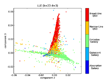
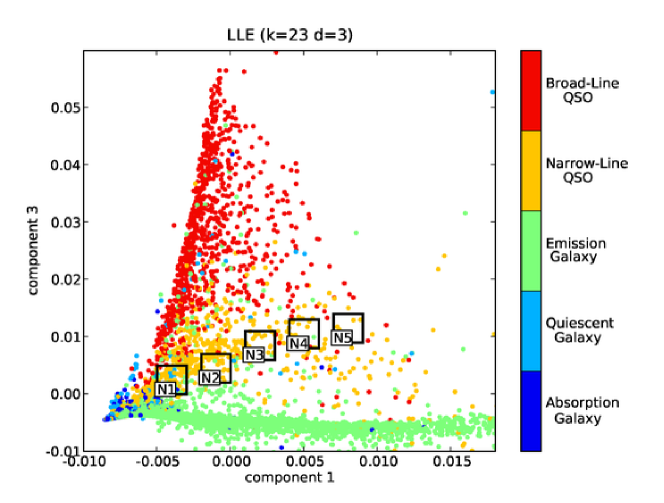
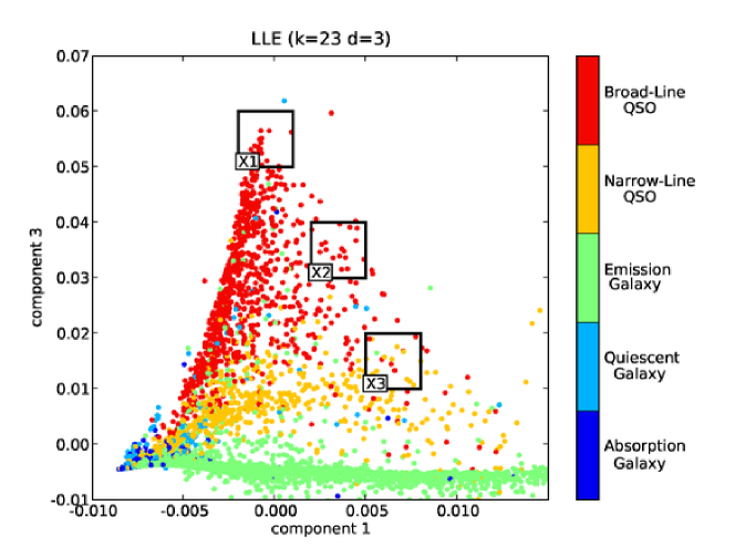
Figure 2 shows the LLE projection of the SDSS spectra from the original 1000 dimensional space to a three dimensional subspace. To minimize the effect of outliers, we use a robust variant of LLE (see section 5.1). We plot the position of all of the sources within this subspace and color-code the points based on the above divisions. Red points are broad-line QSOs, orange points represent narrow-line QSOs, green points are emission-line galaxies and light and dark blue points are galaxies with continuum emission and strong absorption line systems respectively.

The axes of an LLE projection are uniquely defined up to a scaling and a global rotation. The interpretation of the projection comes, therefore, from the relationship between the points rather than from the axes themselves. In Figure 2, it is clear that there are a few well-defined branches in the resulting diagram that separate the sources based on their spectral properties. QSOs (broad and narrow line), emission-line galaxies and continuum galaxies separate in to three basic clusters or classifications. Within these clusters broad and narrow line QSOs can be distinguished as occupying separate parts of the subspace, emission line galaxies are distinct from absorption line systems while the strong absorption line systems closely track the subspace of the continuum galaxies. The positions of galaxies with low emission and absorption line strengths converge to a common region of the 3-dimensional space, which is to be expected as galaxies do not represent a series of individual classifications but rather a continuum of properties.

For the remainder of the paper, all analysis will be done based on the two-dimensional manifold defined by the first and third components (i.e. the larger plot in Figure 2). This sub-projection gives maximal discrimination between the QSO and emission galaxy branches (for further discussion of this choice of projection, see section 5.2).

4.1 Interpretation of the LLE Tracks

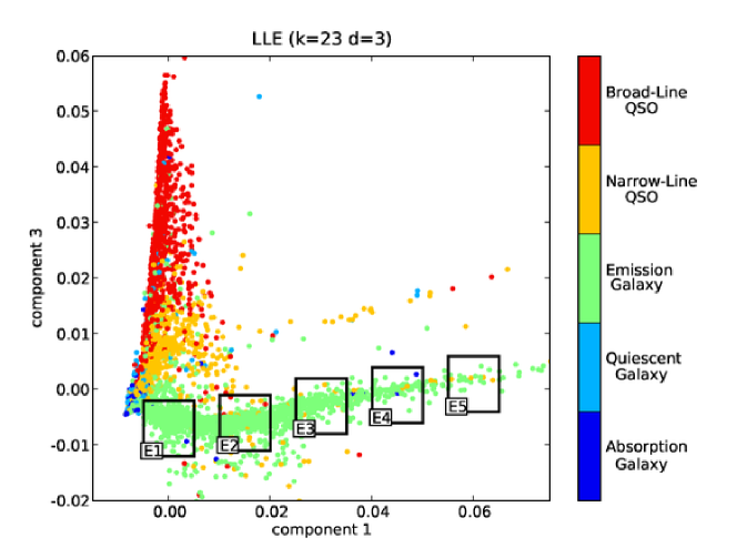
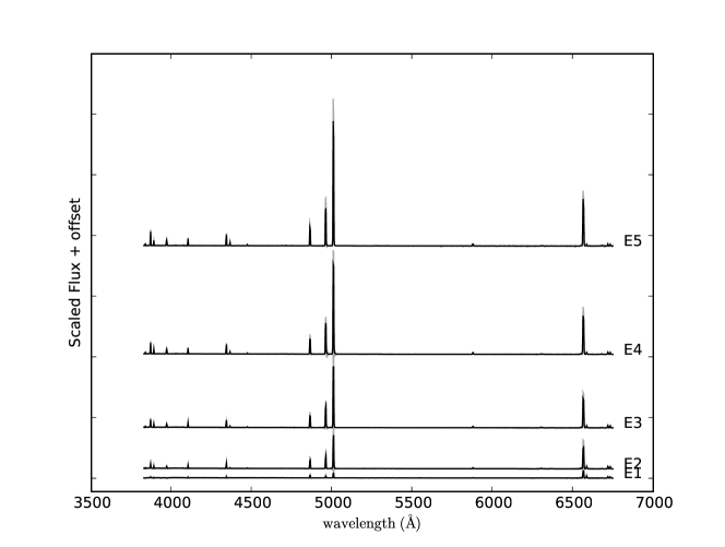
The distance of a galaxy along any one of the branches within Figure 2 correlates well with its physical characteristics (as reflected in their spectra). Figures 3 through 7 show progressions along various regions, along with the mean spectrum of each labeled region. When calculating the mean, we exclude excessively noisy objects, identified as those with flux $F(\lambda)$ satisfying $\int|F(\lambda)|d\lambda>1.5\int F(\lambda)d\lambda$. Because the spectra are preprocessed with a normalization, the few spectra satisfying this inequality would otherwise contribute disproportionately to the mean spectrum in each region.

Figure 3 shows the progression of spectra along the emission galaxy track. To do this we calculate the mean spectrum for galaxies contained within the regions associated with the bounding boxes E1 through E5. As we will show later, this sequence not only tracks increasing line strengths, but also changing line ratios (see Figure 12).

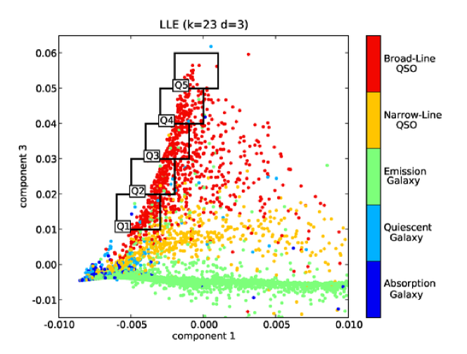
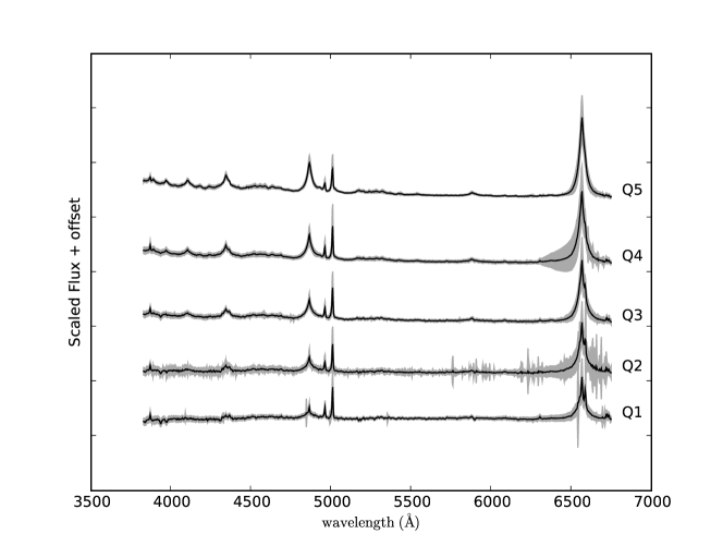
Figure 4 shows the progression of spectra along the broad-line QSO track. We find that, as we move from Q1 to Q5, the spectral type of the QSO evolves from a Seyfert 1.9 to a classic broad line QSO. As would be expected for such a transition the NII emission line strength decreases while the H$\beta$ line strength increases as the spectra become progressively dominated by the accretion disk emission. Associated with these emission line properties we find that the continuum slope of the QSO spectra are bluer for the Q5 class than for Q1. This not only supports the classification of the spectra from Seyfert 1.9 to broad-line AGN, it also demonstrates how LLE can use jointly the information contained within the continuum and line emission.

Figure 5 shows the progression of spectra along the narrow-line QSO track. As with the emission-line galaxy track, the narrow QSO track traces increasing emission from N1 to N5. N1-N3 have narrow H$\beta$ and H$\alpha$, with line-ratios that indicate power-law ionization, and are spectrally consistent with LINERs. N3-N5 have increasingly broad H$\alpha$, which suggests classification as Seyfert 1.9-2.0. Line-ratio diagnostics confirm this (see Figure 12).

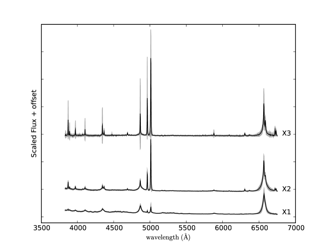
In Figure 6 we consider the progression of spectra across the different spectral groupings (from broad line QSO to galaxies with narrow emission lines) as opposed to along an individual track. The X3 sources are, as before, broad-line QSOs with strong H$\beta$ emission. As we transition to X2 the width of the emission line decreases until X2 has the spectral characteristics of a Seyfert type 1.5. By X1 the spectral properties are consistent with an HII region or narrow emission line galaxy (for wavelengths $<$ 5500 Å) while showing evidence for an AGN component in the broad line H$\alpha$. This one parameter sequence from broad-line QSO to HII region spectra (including regions where the populations are mixed) is described very naturally with this LLE projection.

The last subsample we consider are the quiescent galaxies in Figure 7. The transition from G1 to G5 tracks the same spectral classification from quiescent to active star formation as found using the PCA analysis of Yip et al. (2004a). In terms of spectral properties, galaxies classified as G1 correspond to the E/S0 spectral type from Kennicutt (1998) and galaxies in G5 correspond to the Sbc/Sc Kennicutt spectrum. Along this progression the emission line strengths for H$\alpha$ and NII increase and the strength of the MgIII absorption line decreases. It is also noted that the depth of the break at 4000 Å decreases with increasing index number. Comparisons with the results of Yip et al. (2004a) indicate that this trajectory maps directly to the star formation rate within the galaxy (see Figure 11).

From these initial comparisons it is clear that by projecting onto a three dimensional space using LLE we can differentiate between line-emitting galaxies and those dominated by continuum emission. We can also distinguish between sources as a function of their emission line characteristics. As such, LLE encapsulates both the line emission and continuum emission properties in its classification scheme. That LLE can express the variation in continuum properties of galaxies when projecting from 1000 to 3 dimensions is not altogether surprising as the PCA analyses of Connolly et al. (1995), Yip et al. (2004a) and others have demonstrated that quiescent galaxies occupy only a small region of the available parameter space and that the dominant direction in this space is governed by the star formation rate. For emission line galaxies, and in particular QSOs, standard PCA approaches require between 10 and 50 components to express the variation in line strengths as a function of galaxy type. This is due to the inherently non-linear nature of the reconstruction of emission lines.

The fact that LLE can be used to separate both broad and narrow emission lines into separate groups or families, that the transition between narrow and broad line spectra is smooth, and that the position of a galaxy within each of these groups is dependent on the individual line strengths demonstrates the ability of LLE to concisely represent inherently non-linear systems in an intuitive manner.

Figure 3: Progression of emission galaxy spectra. Each spectrum represents the mean of the spectra within the labeled region. Grey shading indicates the standard deviation about the mean. See caption of Figure 2 for description of colors.

Figure 4: Progression of broad-line QSO spectra. Each spectrum represents the mean of the spectra within the labeled region. Grey shading indicates the standard deviation about the mean. See caption of Figure 2 for description of colors.

Figure 5: Progression of narrow-line QSO spectra. Each spectrum represents the mean of the spectra within the labeled region. Grey shading indicates the standard deviation about the mean. See caption of Figure 2 for description of colors.

Figure 6: Progression from broad to narrow QSO spectra. Each spectrum represents the mean of the spectra within the labeled region. Grey shading indicates the standard deviation about the mean. See caption of Figure 2 for description of colors.

Figure 7: Progression of quiescent galaxy spectra. Each spectrum represents the mean of the spectra within the labeled region. Grey shading indicates the standard deviation about the mean. See caption of Figure 2 for description of colors.

4.2 Separation of Spectral Types

LLE is useful in that it maps a large-dimensional dataset to a smaller dimensional parameter space. Within this projected space, many familiar classification schemes can be applied (see Hastie et al., 2001, for a thorough introduction to the topic). In the case of SDSS spectra, LLE succeeds in mapping physically similar spectra to the same region of parameter space. More importantly, physically different spectra are mapped to distinct, well-separated regions, leading to the possibility of a very intuitive classification scheme.

Because of this, we can quickly locate objects that are misclassified by both the SDSS pipeline and the line-diagnostic plots. Figure 8 displays a few examples of these. M1 is classified by the SDSS pipeline as a broad-line QSO, but falls on the emission-line galaxy track. This mis-classification is likely due to contamination of the H$\alpha$ line from the neighboring Nitrogen features, leading to an erroneous large line-width. M2 is not recognized as an emitting object, because the H$\alpha$ feature is missing. In fact, the entire narrow track on which M2 lies consists of objects which look like emission galaxies/type-2 Seyferts, with the H$\alpha$ line missing due to saturation of the lines, coincident sky lines, and bad pixels. LLE isolates these points on their own track of outliers. M3 and M4 fall on the broad-line QSO track, but are not recognized as broad emitters by the SDSS pipeline, probably due to high background noise. The LLE projection correctly groups these with other strong emitters. Because the LLE projection is entirely neighborhood-based, any given point will have similar properties to nearby points in the projection space.

Next we compare the classification based on LLE to the classification by more traditional methods, e.g. emission line-widths, line-strengths, and line-ratios. This requires a choice of classification technique for points in the LLE-projection space. For illustrative purposes, we create a simple classification scheme and define two well-separated regions which correspond to physically different objects. The “broad-line QSO region” is defined as all points on the broad-line track with LLE component three greater than 0.02. The “emission galaxy region” is defined as all points on the emission galaxy track with LLE component one greater than 0.015 (see figure 2).

Out of the 624 galaxies in the broad-line QSO region, 31 were classified by SDSS as having narrow line emission, and 11 were classified as quiescent. Through visual inspection, 29 of the 31 and 1 of the 11 were found to show broad emission features, with the rest of the spectra too noisy to accurately classify. The SDSS pipeline, therefore, mis-classifies about 5% of their broad-line sources as narrow-line.

Out of the 675 galaxies in the emission galaxy region, 45 have line ratios on the narrow-line QSO side of the Kewley et al. (2001) cutoff, two have H$\alpha$ emission broader than 1200km s^-1, and 4 have prominent emission features not detected by the SDSS pipeline.

Combining the above tallies, we can estimate how successfully LLE clusters physically similar spectra. From a subsample which by design contains a high fraction of abnormal spectra (see Section 5.3), less than one percent of the spectra were physically dissimilar from the average population in each region. These errors are due primarily to very noisy spectra. For other cases, e.g. the 45 spectra where classifications based on LLE and Kewley et al. (2001) line diagnostics disagree, it is not immediately clear which classification is correct, if any. The majority of these sources are transitional, falling near the dividing boundary of the line-ratio diagram. This dividing line is an arbitrary analytic separation between two regions of a certain subset of the parameter space. We note, however, that the LLE-based classification is without any a priori training. We do not preselect sources based on known properties nor fine-tune the parametrization of the classification, as opposed to the optimized SDSS pipelines.

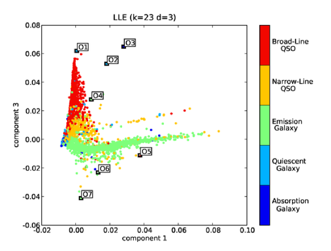
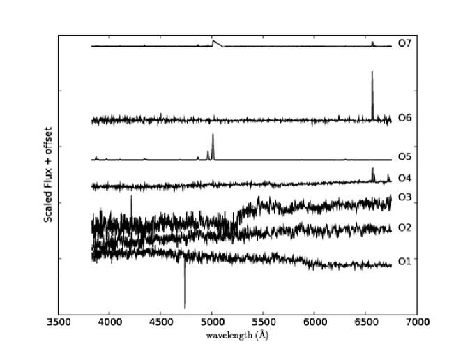
Figure 9 shows a sample of some significant outliers identified with LLE. O1-O3 are outliers due to their noise. O4 and O6 appear to be sky spectra which were misclassified based on emission features. O5 appears to be a QSO with its H$\alpha$ line missing, possibly due to atmospheric absorption. O7 has an artificial feature likely due to faulty sky-noise subtraction. In all of these cases, the spectrum’s status as an outlier based on LLE reflects its unusual spectral characteristics.

Figure 8: A sample of objects with discrepant classifications See caption of Figure 2 for description of colors.

Figure 9: A sample of outliers from the LLE projection See caption of Figure 2 for description of colors.

5 Considerations when applying LLE

5.1 Robust LLE: dealing with noisy and missing data

As with any classification scheme it is important that we can account for missing and noisy data in a robust manner. As LLE is a locally weighted projection it is expected that outliers (even outliers for a single pixel) can impact the definition of the local neighborhood and might bias any classification scheme.

In practice it is difficult to treat this problem completely as it essentially replaces the least squares analysis of each neighborhood with a Total Least Squares/Errors in Variables analysis for each of the $N$ points. These cannot be solved in closed-form, and require a computationally expensive iterative process (see van Huffel & Vandewalle, 1991, for a detailed exploration of the Total Least Squares problem).

We can, however, follow the methodology of Chang & Yeung (2006) and address the problem of outliers using a Robust LLE (RLLE) technique. In RLLE, a reliability score for each data point is determined based on its efficacy in predicting the location of the points in its neighborhood. Outliers will have two general properties: first, they will not be members of large number of local neighborhoods; second, within the neighborhoods in which they appear, they will be far from the best-fit hyperplane. With this in mind, reliability scores are calculated using the following method:

1. For each point, an iteratively reweighted least squares analysis (Holland & Welsch, 1977) is performed to determine optimal weights for a weighted PCA reconstruction of the point from its neighbors. Schematically, this is akin to finding the best-fit hyperplane, weighting points based on their distance from that hyperplane, and repeating until the process converges. As a result of this process, each point in a local neighborhood is assigned a local weight which quantifies its contribution to the local tangent space.

2. Each point may be a member of many neighborhoods. The reliability score for a point is determined by taking the sum of its local weights from each neighborhood of which it is a member.

Thus, a higher score will be given to points which are part of many neighborhoods, and points which contribute more to the reconstruction in each neighborhood. With this in mind, outliers can be identified based on their low reliability score.

In Figure 10 we compare the performance of LLE and RLLE on the S-curve dataset from section 3.2. In this case we assign 15% of the points within the data set to be randomly selected from the full parameter space. The lower left panel shows the application of the standard LLE approach. As is clear from this Figure, outliers can change the local weights of the nearest neighbors and, thereby, distort the resulting lower dimensional manifold; causing the points of different colors to be heavily mixed. Effectively, the random noise within the point distribution fills in enough of the three-dimensional space that LLE cannot extract the lower dimensional manifold. For RLLE, as long as the number of random points is small relative to the number of nearest neighbors, we can isolate and exclude the contaminating points from the local weights. Figure 10 shows that we can recover the underlying two-dimensional manifold in the presence of noise and outliers through this approach.

Figure 10: Top: $N=2000$ points randomly sampled from a bounded 2-manifold embedded in 3-space, with 15% of the points random outliers sampled from the entire parameter space. Bottom Left: the 2-dimensional LLE projection of this manifold, with $k=15$. Note the mixing of the colors: the outliers obscure the 2-dimensional manifold to the point that LLE cannot recover it. Bottom Right: the 2 dimensional RLLE projection of this manifold, with $k=15$, constructed using 80% of the points with the highest reliability scores. RLLE recovers the desired projection.

5.2 Choosing Optimal Parameters

There are three free parameters that must be chosen for LLE: $K$, the number of nearest neighbors, $D_{out}$, the output dimension, and $r$, the regularization parameter. $K$ and $D_{out}$ will be discussed here, while $r$, which depends on details of the implementation, is addressed in appendix B.

Often in PCA, instead of specifying an output dimension $D_{out}$, one chooses to specify a percentage of the sample variance which should be preserved. In LLE, dimensionality can be determined in an analogous way for each local neighborhood (de Ridder & Duin, 2002). In the computation of an LLE projection, a variant of the covariance matrix is computed for each local neighborhood. This matrix differs from the covariance matrix used in PCA by only a translation and scaling, neither of which affect the relative magnitudes of the eigenvalues. Taking the lead from PCA, we can specify a percentage of the local variance which we would like to conserve, and thereby find the minimum number of dimensions required locally, simply by doing an eigenanalysis of the local covariance matrix. Taking the mean of the $N$ local dimensionality determinations gives an estimate of the optimal value of $D_{out}$ for the global projection. For our SDSS analysis, the first three components contain an average of 75% of the local variance. The first ten components contain 92% of the local variance, significantly less than the 99.9% of total variance within the first ten PCA eigenspectra of Yip et al. (2004a). This discrepancy is likely due to noise and intrinsic variation at the local level, which contributes more to the small, local neighborhoods which LLE probes than to the overall variance that PCA probes. Also, our sampling technique (Section 5.3) chooses sources based on dissimilarity, leading to more intrinsic variation in the subsample.

Choosing the number of nearest neighbors is more difficult. In fact, $K$ need not be constant across all neighborhoods. It could be specified based on local properties of the manifold or the density of sources at a given point. The literature on LLE offers no consensus on how to choose the optimal value of $K$. Too large a value, and the manifold is oversampled, destroying the assumption of local linearity, and leading to an inherently larger dimensional space. Too low, and the manifold is undersampled, which leads to a loss of information on the relationships between neighborhoods and more sensitivity to the presence of outliers and noise. In this work we take an empirical approach and try to estimate a series of heuristics that can be applied to the spectral data. We take a range of values for $K$ ($10<K<30$) and determine our ability to maximally distinguish between galaxy populations in the resulting LLE classifications. In the case of galaxy spectra, the $K$ is chosen which maximizes the opening angle between the QSO and emission-line galaxy sequences, measured between any two of the three leading projection dimensions. We find that a value of $K=23$ provides the maximal discrimination but that values of $K$ from 20 to 27 are comparable.

It should be noted that the final LLE projection is unique only up to a global translation and rotation. Because of this, the exact nature of the projection is highly dependent on the subset of data chosen, as well as the above-mentioned input parameters. What is invariant, however, is the relationship between each point and its neighbors. In particular, an outlying point in one projection will be an outlier in another projection. This is what makes LLE useful: it allows one to easily visualize the relationships between points in a high-dimensional parameter space.

5.3 Fast LLE: efficient sampling strategies

The LLE algorithm, even when optimized, is computationally expensive. The main bottleneck is the neighbor search, which, for a single point is $\mathcal{O}[ND_{in}]$. Using brute-force for all $N$ points is, at worst, $\mathcal{O}[N^{2}D_{in}]$. While more advanced tree-based algorithms can significantly improve on this, it remains a computational hurdle, especially for high-dimensional datasets (see Berchtold et al., 1998, for a review of fast nearest-neighbor algorithms).

The second bottleneck is the computation of the global projection, which involves determining the bottom $D_{out}+1$ eigenvectors of a $[N\times N]$ sparse matrix (see appendix C). By using iterative techniques such as Arnoldi/Lanczos Decomposition, it is possible to determine these eigenvectors without performing a full matrix diagonalization (see Wright & Trefethen, 2001, for one well-tested optimized algorithm).

Even fully optimized, it is not feasible to learn the LLE projection from the full SDSS spectral sample, which would amount to hundreds of thousands of points in a 4000-dimensional dataspace. What is more, a random subsample of these data will be too sparsely populated in some regions of space (e.g. for strong line emitters that account for $<0.01$% of a randomly sample of spectra from the SDSS), and too densely populated in others (e.g. around L^∗ galaxies). In this case LLE will not sufficiently probe the entire structure of the manifold. For this reason, a strategy is needed to define a subsample that best spans the entire parameter space, without overpopulating the most probable neighborhoods.

To do this, we follow de Ridder & Duin (2002) and appeal to the fundamental assumption of local linearity on the manifold. For a given point $\mathbf{x_{i}}$, the first step of LLE is to compute the weights required to construct it from its $K$ neighbors. The procedure outlined in section 5.2 for determining the intrinsic dimensionality can be used to find the local reconstruction error: i.e., the percentage of total variance not captured in the $D_{in}$-dimensional projection. Points for which this local projection error is small add very little information to the overall projection. They can be discarded without much effect. Points for which this reconstruction error is large are not well-approximated by a linear combination of neighbors, and, therefore, contain information not present in the local best-fit hyperplane. If they are thrown out, the projected manifold will change significantly.

With this in mind, the following strategy was used to reduce the $\sim 170,000$ unique spectra to a manageable $9,000$:

1. Divide the sample into groups of $2000$ spectra each.

2. For each group:

   1. find the eigenvalues of the local covariance matrix of each point, and create a cumulative distribution based on the local reconstruction error.

   2. randomly select 20% of the points based on this cumulative distribution, such that those with the largest reconstruction error are preferentially selected.

3. merge every 5 subsamples into a new sample of $2000$ spectra

4. repeat this procedure until the total subsample is of the desired size.

5.4 Applying LLE to new data sets

Once the projection is determined for a given training sample, it is straightforward to determine the projection of new data onto the training surface. For each new point, the $K$ nearest neighbors are determined within the training data. Weights are determined by minimizing the form of Equation 2. These weights are then used within Equation 4 to determine the projection of the point. Note that this second step amounts to nothing more than a weighted sum of the projected neighbors. This is a key point in the application of LLE: once a projection is defined for a representative training sample, the computational cost of the classification of a set of test-points is largely due to a $K$-nearest-neighbor search within the training set. This can be done optimally in $\mathcal{O}[D_{in}\log N]$.

Reconstructing unknown data from projected coordinates requires the reverse of the above procedure. Weights are determined by minimizing the corollary of Equation 2 within the projected space, and these weights are used to reconstruct the point in the original data space.

6 Discussion

As we have shown in section 4, LLE provides an efficient and automated way of classifying high dimensional data (in our case galaxy spectra) that can account for inherent non-linearities within these data. For spectroscopic observations LLE can jointly classify spectra based on their emission-line and continuum properties which makes it well suited to the task of automated classification for large spectroscopic surveys. In the following section we compare the output from the LLE classifications with those from standard spectral classification techniques and discuss how LLE might be adopted for the next generation of spectroscopic surveys.

Figure 11 shows the PCA mixing-angle plot using the publicly available Yip et al. (2004a) SDSS galaxy eigenspectra (see Figure 8 in that work). The average spectral sequences from Figures 3-7 are over-plotted for comparison. As discussed by Yip et al. (2004a), $\phi_{KL}$ correlates with spectral type (see also Connolly et al., 1995) or star formation rate. It is, however, not well-suited to distinguishing between various types of line emission: broad-line QSOs, narrow-line QSOs, and emission-line galaxies overlap the same region of the projection space. This is a reflection of the fact that PCA is sensitive to continuum information rather than to line emission. Accounting for line emission in a PCA framework requires extracting the emission lines and applying PCA to the line equivalent widths (Györy et al., 2008).

Figure 11: Principal component mixing-angle diagram for the SDSS spectra subsample. The labeled tracks correspond to average spectra plotted in figures 3-7. See caption of Figure 2 for description of colors.

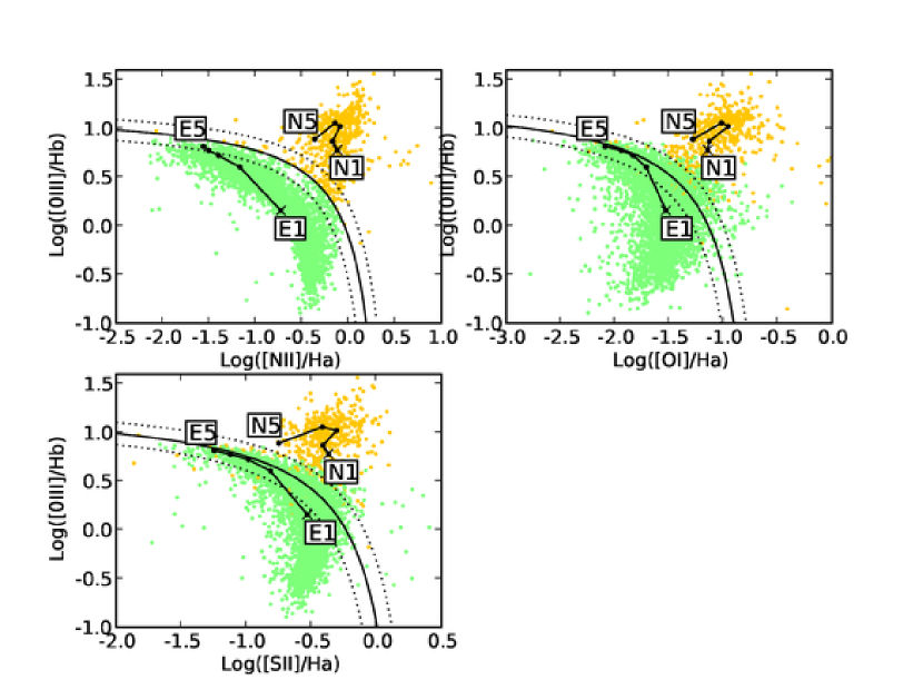
Figure 12 shows the typical line-ratios used to distinguish between star-forming galaxies and narrow-line QSOs. The dividing lines between the populations are due to Kewley et al. (2001). The tracks on the plot correspond to the average spectra in Figures 3 and 5 (Note that line-ratio diagrams do not meaningfully classify broad-line QSOs, which uniformly occupy the entire space of the line-ratio plots). Kewley et al. (2001) use stellar synthesis models to show that emission characteristics of the objects below the dividing line can be attributed to ionization due to young stellar populations, with the ionization parameter $q$ increasing toward the upper-left. This gives a physical interpretation of the emission galaxy (E) sequence of Figure 3: increasing star formation from E1 to E5.

The region above the dividing line, therefore, is due to ionization which cannot be attributed to star formation. Ho et al. (1997) show empirically that this region can be subdivided into transitional objects near the dividing line, LINERs which lie near N1-N2, and Seyfert-2 galaxies which lie near N3-N5. The narrow-line QSO (N) sequence of Figure 5 traces this transition.

Figure 12: Line-ratio diagram of the objects in the subsample which display $3\sigma$ emission with a width $<1200km$. Points above the cutoff are considered narrow-line QSOs, while points below the cutoff are considered emission-line galaxies. Note that broad-line QSOs are not meaningfully classified by these diagrams, and are omitted. Lines show the boundaries between narrow-line QSOs and star-forming galaxies given in Kewley et al. (2001). The tracks labeled E and N are the average spectra from Figures 3 and 5, respectively.

The above discussion points to the usefulness of LLE for automatic classification, without requiring the extraction of line parameters from the spectroscopic data. As with most classification schemes, the bulk of the work happens in the training of the LLE. Once the projection parameters (Section 5.2) and training subsample (Section 5.3) are chosen, the resulting projection provides the basis for a unique, repeatable classification scheme, with computational cost dominated by a $K$-nearest neighbor search within the training sample (Section 5.4). As such LLE can provide an accurate initial classification and anomaly detection step for any automated spectroscopic pipeline, requiring only the extraction of spectroscopic redshifts.

LLE is not limited to spectroscopic information. In principle, LLE can be used to visualize any type of data, even non-homogeneous data sets, e.g. a combination of fluxes, redshifts, angular size, etc. Care must be taken, though, to make sure that non-homogeneous dimensions contribute equally to the nearest neighbor search. This can be assured through modification of the distance metric for the nearest-neighbor search such that the distance between point $\mathbf{x}$ and point $\mathbf{y}$ are

$$d_{\mathbf{xy}}=\sqrt{\sum_{i}w_{i}(x_{i}-y_{i})^{2}}$$ (6)

where $w_{i}$ is a weight associated with measurement dimension $i$. For example, if the measurements in question are fluxes that range from $0$ to $1000$ and redshifts that range from $0$ to $1$, $w_{i}$ could be set to reflect the parameter range: $w_{i}=[\max(x_{i})-\min(x_{i})]^{-1}$. This normalization of the data prior to the LLE step is common to any dimensional reduction technique, including PCA.

The computational cost of learning the LLE required that we develop a subsampling technique that preserves the complexity of the underlying data (i.e. as opposed to a random sampling that will be dominated by the typical sources within a population). Neighborhood-based subsampling is important in two key areas: it yields a subsample which fills the entire observational parameter space, and the data are uniformly sampled throughout. Furthermore, the local nature of the process means that subtle nonlinear effects are not obscured in the process. This subsampling technique, described in Section 5.3, is broadly applicable, regardless of the classification scheme being employed. It could be applied to any problem that requires sampling of a large data set – such as spectroscopic follow-up of optical or radio selected galaxies or spectroscopic observations of galaxies for training galaxy photometric redshifts.

7 Conclusions

Fast classification of large data sets is an increasingly present problem in astronomy. With this paper we show Locally Linear Embedding to be a powerful tool in the classification SDSS spectra that is sensitive to both low-frequency and high-frequency information. As such, is an improvement over standard techniques such as PCA/KL decomposition and line-ratio diagnostics. LLE is still in its infancy, and more understanding is needed to take into account measurement uncertainties, missing data, and undersampled manifolds. We discuss the limitations of LLE due to the computational cost of operating on large data sets and how these can be addressed through intelligent sampling of the training data. Our sampling technique is based on local information content and yields a training subsample which preserves the nonlinear traits of the sample as a whole. As a dimensionality reduction technique, LLE is both fast and accurate, and sensitive to all the information contained in measurement data. Because of this, it has potential to become a useful step in efficient classification of large astronomical data sets.

LLE software used in this paper is publicly available at http://ssg.astro.washington.edu/software (see appendix E).

Appendix A Notational Conventions

Throughout this paper, matrices are denoted by bold capital letters ($\mathbf{X}$, $\mathbf{Y}$, etc.), vectors are given by bold lowercase letters ($\mathbf{x}$, $\mathbf{y}$, etc.), while scalar values are in normal-face type ($X$, $y$, $\lambda$, etc.). Subscripts reference the individual elements of matrices, such that $X_{ij}$ is the element in the $i$th row and $j$th column of matrix $\mathbf{X}$. The $i$th column vector of matrix $\mathbf{X}$ is given by $\mathbf{x_{i}}$. Note the potential for confusion with this convention: $(\mathbf{x_{j}})_{i}=X_{ij}$. To limit this source of confusion, individual elements of a matrix will always be referenced via the latter formulation. $\mathbf{I}$ is the square identity matrix, such that $I_{ij}=\delta_{ij}$, where $\delta_{ij}$ is the Kroniker delta function. $\mathbf{0}$ is the zero matrix, such that $0_{ij}=0$ for all $i$ and $j$. The sizes of these two matrices should be clear from the context in which they are used. The derivations in the following sections are based on those found in Roweis & Saul (2000) and de Ridder & Duin (2002), with the addition of a few clarifying details.

Appendix B Determining the Optimal Weights

The optimal weights $\mathbf{w}^{(i)}$ are determined by minimizing the reconstruction error given in equation 2:

$$\mathcal{E}_{1}^{(i)}(\mathbf{w}^{(i)})=\Bigg{|}\mathbf{x_{i}}-\sum_{j=1}^{K}w_{j}^{(i)}\mathbf{x}_{n_{j}^{(i)}}\Bigg{|}^{2}$$ (B1)

This can be straightforwardly solved in closed form, using the method of Lagrangian multipliers. Consider a neighborhood about the point $x_{i}$, with weights $w_{j}$ that satisfy

$$\sum_{j=1}^{K}w^{(i)}_{j}=1.$$ (B2)

This constraint is useful because it imposes translational invariance to the projection. Using this condition, the above sum can be rewritten

$$\mathcal{E}_{1}^{(i)}(\mathbf{w}^{(i)})=\Bigg{|}\sum_{j=1}^{K}w_{j}^{(i)}\Big{(}\mathbf{x_{i}}-\mathbf{x}_{n_{j}^{(i)}}\Big{)}\Bigg{|}^{2}.$$ (B3)

Now defining the local covariance matrix

$$C^{(i)}_{jk}=\Big{(}\mathbf{x_{i}}-\mathbf{x}_{n_{j}^{(i)}}\Big{)}^{T}\Big{(}\mathbf{x_{i}}-\mathbf{x}_{n_{k}^{(i)}}\Big{)}$$ (B4)

We find

$$\mathcal{E}_{1}^{(i)}(\mathbf{w}^{(i)})=\sum_{j=1}^{K}\sum_{k=1}^{K}w_{j}^{(i)}w_{k}^{(i)}C^{(i)}_{jk}$$ (B5)

We can minimize this by applying a Lagrange multiplier $\lambda_{i}$ to enforce the constraint given in equation B2:

$$\mathcal{E}_{1}^{(i)}(\mathbf{w}^{(i)})=\sum_{j=1}^{K}\sum_{k=1}^{K}w_{j}^{(i)}w_{k}^{(i)}C^{(i)}_{jk}+2\lambda_{i}\Big{(}1-\sum_{j}w_{j}^{(i)}\Big{)}$$ (B6)

Minimizing $\mathcal{E}_{1}^{(i)}(\mathbf{w}^{(i)})$ with respect to $\mathbf{w}^{(i)}$ gives the condition of minimization:

$$\mathbf{C}^{(i)}\mathbf{w}^{(i)}=\lambda_{i}\mathbf{\vec{1}},$$ (B7)

where $\mathbf{\vec{1}}=[1,1,...1]^{T}$. Defining $\mathbf{R}^{(i)}$ to be the inverse of the local covariance matrix $\mathbf{C}^{(i)}$, we are left with

$$\mathbf{w}^{(i)}=\lambda_{i}\mathbf{R}^{(i)}\mathbf{\vec{1}}$$ (B8)

Now imposing the constraint (B2) leads to

$$\lambda_{i}=\Big{(}\sum_{j=1}^{N}\sum_{k=1}^{N}R^{(i)}_{jk}\Big{)}^{-1}.$$ (B9)

Evaluation of $\mathbf{w}^{(i)}$ with equations B8 and B9 requires explicit inversion of the local covariance matrix. In practice, a more efficient method of calculation is to solve a variation of equation B7,

$$\mathbf{C}^{(i)}\mathbf{w}^{(i)}=[1,1,1...1]^{T},$$ (B10)

and then rescale the resulting $\mathbf{w}^{(i)}$ such that the constraint in equation B2 is satisfied.

In general, the local covariance matrix $\mathbf{C}^{(i)}$ may be nearly singular. In this case, the weights $\mathbf{w}^{(i)}$ are not well defined. de Ridder & Duin (2002) note that the matrix can be regularized based on its eigenvalues $\mathbf{\lambda}^{(i)}$. Because, in the end, we are doing a global projection to a dimension $D_{out}$, we can follow probabilistic PCA and define

$$r=\frac{1}{K-D_{out}}\sum_{j=D_{out}+1}^{K}\lambda_{j}^{(i)},$$ (B11)

i.e., the mean of the eigenvalues of the unused eigenvectors, and regularize our matrix as $\mathbf{C}^{(i)}=\mathbf{C}^{(i)}+r\mathbf{I}$. In practice, this would require an explicit eigenvalue decomposition for each local covariance matrix, which is very computationally expensive. We can obtain a similar regularization parameter by noting that $\sum\lambda_{i}={\rm tr}(\mathbf{C}^{(i)})$. If our $D_{out}$-dimensional projection contains the majority of the variance (which, under the assumptions of the algorithm, it should), we see that $r$ will be very small compared to the trace of $\mathbf{C}^{(i)}$. For this paper, the value $r=(10^{-3}){\rm tr}(\mathbf{C}^{(i)})$ was used.

Appendix C Determining The Optimal Projection

The projection error is given by equation 4:

$$\mathcal{E}_{2}(\mathbf{Y})=\sum_{i=1}^{N}\Bigg{|}\mathbf{y_{i}}-\sum_{j=1}^{K}w_{j}^{(i)}\mathbf{y}_{n_{j}^{(i)}}\Bigg{|}.$$ (C1)

To simplify this, we define a sparse weight matrix $\mathbf{W}$ with columns populated by the weight vectors $\mathbf{w}^{(i)}$, such that

$$W_{ik}=\left\{\begin{array}[]{ll}w_{j}^{(i)}&\mathrm{if\ }k=n_{j}^{(i)}\\ 0&\mathrm{if\ }k\notin\mathbf{n}^{(i)}\end{array}\right.$$ (C2)

The projection error can then be rewritten in a more compact form:

$$\mathcal{E}_{2}(\mathbf{Y})=\Big{|}\mathbf{Y}-\mathbf{Y}\mathbf{W}\Big{|}^{2}.$$ (C3)

It can be shown that this is equivalent to the quantity

$$\mathcal{E}_{2}(\mathbf{Y})=\mathrm{tr}\Big{(}\mathbf{YMY}^{T}\Big{)},$$ (C4)

where we have defined

$$\mathbf{M}=(\mathbf{I}-\mathbf{W})(\mathbf{I}-\mathbf{W})^{T}.$$ (C5)

It is clear that equation C4 is trivially minimized by $\mathbf{Y}=\mathbf{0}$. In order to find solutions of interest, we will impose the constraint

$$(\mathbf{YY}^{T})=\mathbf{I}.$$ (C6)

That is, the rows of $\mathbf{Y}$ are orthonormal. We can then use Lagrangian multipliers $\lambda_{i}$ to constrain equation C4:

$$\mathcal{E}_{2}(\mathbf{Y})=\mathrm{tr}\Big{(}\mathbf{YMY}^{T}+\mathbf{\Lambda}(\mathbf{I}-\mathbf{YY}^{T})\Big{)}$$ (C7)

where $\mathbf{\Lambda}$ is the diagonal matrix of Lagrangian multipliers, with $\Lambda_{ii}=\lambda_{i}$. Minimizing this with respect to $\mathbf{Y}$ gives the condition

$$\mathbf{MY}^{T}-\mathbf{Y}^{T}\mathbf{\Lambda}=\mathbf{0},$$ (C8)

Denoting the rows of $\mathbf{Y}$ with the vectors $\mathbf{y}^{(i)}$, this can be written in a more familiar form:

$$\mathbf{My}^{(i)}-\lambda_{i}\mathbf{y}^{(i)}=\mathbf{0}.$$ (C9)

We see that $\lambda_{i}$ and $\mathbf{y}^{(i)}$ are simply the eigenvalues and eigenvectors of the symmetric-real matrix $\mathbf{M}$. Equation C8 can then be rewritten $\mathbf{YMY}^{T}=\mathbf{\Lambda}$ and our reconstruction error (C4) is simply

$$\mathcal{E}_{2}(\mathbf{Y})=\mathrm{tr}(\mathbf{\Lambda})=\sum_{i}\lambda_{i}.$$ (C10)

Evidently, the desired projection is contained in the eigenvectors of $\mathbf{M}$ corresponding to the smallest eigenvalues. Because of the constraint in equation B2, it is clear that $\mathbf{y}^{(0)}\propto[1,1,1,...1]^{T}$ is a solution with eigenvalue $\lambda_{0}=0$. This solution amounts to a translation in space, and can be neglected.

Thus, we see that the $D_{out}$-dimensional projection $\mathbf{Y}$ of a data matrix $\mathbf{X}$ is given simply by the $(D_{out}+1)$-dimensional null-space of matrix $\mathbf{M}=(\mathbf{I}-\mathbf{W})(\mathbf{I}-\mathbf{W})^{T}$, with the lowest eigenvector neglected.

Fortunately, a full matrix diagonalization is not necessary to find only a few extreme eigenvectors. Iterative methods such as Arnoldi decomposition or Lanczos factorization can be used to determine this null-space rather efficiently. What is more, though the matrix $\mathbf{I}-\mathbf{W}$ is a sparse $[N\times N]$ matrix, with only $K+1$ nonzero entries per column. Thus, the LLE algorithm has large potential for optimization in both computational and storage requirements.

Appendix D LLE Algorithm

Here is a description of the basic LLE algorithm, taking into account the above discussion. Given $N$ points in $D_{in}$ dimensions, to be projected to $D_{out}$ dimensions, using the $K$ nearest neighbors of each point:

1. for $i=1\to N$

   1. find the $K$ nearest neighbors of point $i$

   2. construct the local covariance matrix, $\mathbf{C}^{(i)}$ (eqn. B4)

   3. regularize the local covariance matrix by adding a fraction of its trace to the diagonal: $\mathbf{C}^{(i)}=\mathbf{C}^{(i)}+\delta\cdot{\rm tr}(\mathbf{C}^{(i)})\mathbf{I}$. Choosing $\delta=10^{-3}$ works well in practice (See appendix B.)

   4. determine $\mathbf{w}^{(i)}$ by solving equation B10.

   5. use $\mathbf{w}^{(i)}$ to populate column $i$ of the weight matrix $\mathbf{W}$, with $W_{ji}=0$ if point $j$ is not a neighbor of point $i$.

2. Construct the matrix $\mathbf{M}=(\mathbf{I}-\mathbf{W})(\mathbf{I}-\mathbf{W})^{T}$

3. Determine the $D_{out}+1$ eigenvectors of matrix $\mathbf{M}$ corresponding to the smallest eigenvalues. The LLE projection is given by these, neglecting the lowest (which is merely a translation).

Appendix E Description of DimReduce code

DimReduce is a C++ code which performs LLE and some of its variants on large datasets. To handle the computationally intensive pieces of the algorithm, it includes a basic interface to the optimized FORTRAN routines in BLAS, LAPACK, and ARPACK.

The DimReduce interface works with data saved in the FITS format, a commonly used binary file format used for astronomical images and data. Four variants of LLE are available:

LLE:

This is the basic LLE algorithm. The user must provide input data, the number of nearest neighbors, and either the output dimension or a desired variance to preserve within each neighborhood.

HLLE:

This is a variant of LLE which uses a Hessian estimator within each neighborhood which better preserves angles in each neighborhood. The algorithm is based on Donoho & Grimes (2003). Inputs are similar to LLE, with the added restriction that $K$ must be larger than $D_{in}$, the input dimension.

RLLE1:

This is a robust variant of LLE, based on an algorithm outlined in Chang & Yeung (2006). To detect outliers, an iteratively reweighted PCA is performed on each neighborhood. A reliability score is assigned to each point based on the number of neighborhoods in which it appears, as well as its iteratively determined contribution within each neighborhood. The user provides inputs similar to those of LLE, as well as an reliability cutoff: a number between zero and one that represents the fraction of points believed to be outliers.

RLLE2:

This is another robust variant of LLE outlined in Chang & Yeung (2006), where outliers are handled on a neighborhood by neighborhood basis. Reliability scores are computed as described above, and within each neighborhood the nearest $K+R$ nearest neighbors are found, and then the $R$ neighbors with the lowest reliability scores are discarded. The user provides inputs similar to those of LLE, as well as the number $R$ of excess neighbors to find within each neighborhood.

LLEsig:

This is a utility routine which can be used in the data selection procedure described in section 5.3. Given an input matrix, a number of nearest neighbors, and an output dimension, this will compute the local linear reconstruction error for each point. The result is the local reconstruction error for each point.

In addition, a python utility is provided to plot and examine the results, using the open source packages scipy and matplotlib. All of the source code is available on the web, along with test data and example scripts.

There are a few possible optimizations to DimReduce which have not yet been implemented. First of all, the sparse weight matrix is presently stored in dense format. Storage requirements and execution time could be greatly reduced by taking advantage of its sparsity. Secondly, the $K$-nearest neighbor search is presently performed using a non-optimized brute-force algorithm. Use of a ball-tree, cover-tree, or similar algorithm would greatly speed up the performance, especially when projecting new test data onto a training surface. Thirdly, the entire package could be fairly easily restructured to take advantage of parallel computing capabilities. Parallelized versions of BLAS, LAPACK, and ARPACK are all publicly available, and the computation of nearest neighbors and construction of the weight matrix lends itself easily to parallelization. Implementation of these improvements, along with the use of the data sampling strategies outlined in section 5.3 give LLE the possibility of being used for automated classification of objects in a large variety of contexts.

References

- Abazajian & Sloan Digital Sky Survey (2008) Abazajian, K., & Sloan Digital Sky Survey, f. t. 2008, ArXiv e-prints
- Abraham et al. (1994) Abraham, R. G., Valdes, F., Yee, H. K. C., & van den Bergh, S. 1994, ApJ, 432, 75
- Abraham et al. (2003) Abraham, R. G., van den Bergh, S., & Nair, P. 2003, ApJ, 588, 218
- Bailer-Jones et al. (1998) Bailer-Jones, C. A. L., Irwin, M., & von Hippel, T. 1998, MNRAS, 298, 361
- Baldwin et al. (1981) Baldwin, J. A., Phillips, M. M., & Terlevich, R. 1981, PASP, 93, 5
- Berchtold et al. (1998) Berchtold, S., Ertl, B., Keim, D. A., peter Kriegel, H., & Seidl, T. 1998, in In Proceedings of the 14th International Conference on Data Engineering, 209–218
- Boroson & Green (1992) Boroson, T. A., & Green, R. F. 1992, ApJS, 80, 109
- Bromley et al. (1998) Bromley, B. C., Press, W. H., Lin, H., & Kirshner, R. P. 1998, ApJ, 505, 25
- Bruzual & Charlot (2003) Bruzual, G., & Charlot, S. 2003, MNRAS, 344, 1000
- Budavári et al. (2009) Budavári, T., Wild, V., Szalay, A. S., Dobos, L., & Yip, C.-W. 2009, MNRAS, 394, 1496
- Chang & Yeung (2006) Chang, H., & Yeung, D.-Y. 2006, Pattern Recogn., 39, 1053
- Connolly et al. (1995) Connolly, A. J., Szalay, A. S., Bershady, M. A., Kinney, A. L., & Calzetti, D. 1995, AJ, 110, 1071
- Conselice (2003) Conselice, C. J. 2003, VizieR Online Data Catalog, 214, 70001
- Cramer & Maeder (1979) Cramer, N., & Maeder, A. 1979, A&A, 78, 305
- de Ridder & Duin (2002) de Ridder, S., & Duin, R. 2002, Pattern Recognition Group, Department of Science and Technology, Delft University of Technology, Technical Report PH-2002-01
- de Vaucouleurs (1959) de Vaucouleurs, G. 1959, Handbuch der Physik, 53, 275
- Donoho & Grimes (2003) Donoho, D. L., & Grimes, C. 2003, PNAS, 100, 5591
- Efstathiou & Fall (1984) Efstathiou, G., & Fall, S. M. 1984, MNRAS, 206, 453
- Einbeck et al. (2007) Einbeck, J., Evers, L., & Bailer-Jones, C. 2007, ArXiv e-prints
- Ferreras et al. (2006) Ferreras, I., Pasquali, A., de Carvalho, R. R., de la Rosa, I. G., & Lahav, O. 2006, MNRAS, 370, 828
- Folkes et al. (1999) Folkes, S. et al. 1999, MNRAS, 308, 459
- Folkes et al. (1996) Folkes, S. R., Lahav, O., & Maddox, S. J. 1996, MNRAS, 283, 651
- Francis et al. (1992) Francis, P. J., Hewett, P. C., Foltz, C. B., & Chaffee, F. H. 1992, ApJ, 398, 476
- Fukugita et al. (1996) Fukugita, M., Ichikawa, T., Gunn, J. E., Doi, M., Shimasaku, K., & Schneider, D. P. 1996, AJ, 111, 1748
- Galaz & de Lapparent (1998) Galaz, G., & de Lapparent, V. 1998, A&A, 332, 459
- Gulati et al. (1999) Gulati, R. K., Bravo, A., Padilla, G., & Altamirano R, L. 1999, in IAU Symposium, Vol. 192, The Stellar Content of Local Group Galaxies, ed. P. Whitelock & R. Cannon, 369–+
- Gunn et al. (1998) Gunn, J. E. et al. 1998, AJ, 116, 3040
- Györy et al. (2008) Györy, Z., Szalay, A. S., Budavári, T., Csabai, I., & Charlot, S. 2008, submitted to Astronomical Journal
- Hastie et al. (2001) Hastie, T., Tibshirani, R., & Friedman, J. 2001, The Elements of Statistical Learning, Springer Series in Statistics (New York, NY, USA: Springer New York Inc.)
- Heavens et al. (2000) Heavens, A. F., Jimenez, R., & Lahav, O. 2000, MNRAS, 317, 965
- Ho et al. (1997) Ho, L. C., Filippenko, A. V., & Sargent, W. L. W. 1997, ApJS, 112, 315
- Holland & Welsch (1977) Holland, P. W., & Welsch, R. E. 1977, Comm. Statistics Theory and Methods
- Kaiser et al. (2002) Kaiser, N. et al. 2002, in Society of Photo-Optical Instrumentation Engineers (SPIE) Conference Series, Vol. 4836, Society of Photo-Optical Instrumentation Engineers (SPIE) Conference Series, ed. J. A. Tyson & S. Wolff, 154–164
- Kennicutt (1998) Kennicutt, Jr., R. C. 1998, ARA&A, 36, 189
- Kewley et al. (2001) Kewley, L. J., Dopita, M. A., Sutherland, R. S., Heisler, C. A., & Trevena, J. 2001, ApJ, 556, 121
- Kunzli et al. (1997) Kunzli, M., North, P., Kurucz, R. L., & Nicolet, B. 1997, A&AS, 122, 51
- Lahav et al. (1996) Lahav, O., Naim, A., Sodré, Jr., L., & Storrie-Lombardi, M. C. 1996, MNRAS, 283, 207
- Madgwick et al. (2003a) Madgwick, D. S. et al. 2003a, ApJ, 599, 997
- Madgwick et al. (2003b) Madgwick, D. S., Hewett, P. C., Mortlock, D. J., & Wang, L. 2003b, ApJ, 599, L33
- Madgwick et al. (2003c) Madgwick, D. S., Somerville, R., Lahav, O., & Ellis, R. 2003c, MNRAS, 343, 871
- Osterbrock & De Robertis (1985) Osterbrock, D. E., & De Robertis, M. M. 1985, PASP, 97, 1129
- Reichardt et al. (2001) Reichardt, C., Jimenez, R., & Heavens, A. F. 2001, MNRAS, 327, 849
- Richards et al. (2009) Richards, J. W., Freeman, P. E., Lee, A. B., & Schafer, C. M. 2009, ApJ, 691, 32
- Ronen et al. (1999) Ronen, S., Aragon-Salamanca, A., & Lahav, O. 1999, MNRAS, 303, 284
- Roweis & Saul (2000) Roweis, S., & Saul, L. 2000, Science, 290, 2323
- Schneider et al. (2008) Schneider, D. P. et al. 2008, VizieR Online Data Catalog, 7252, 0
- Singh et al. (1998) Singh, H. P., Gulati, R. K., & Gupta, R. 1998, MNRAS, 295, 312
- Skrutskie et al. (2006) Skrutskie, M. F. et al. 2006, AJ, 131, 1163
- Sodre & Cuevas (1997) Sodre, L., & Cuevas, H. 1997, MNRAS, 287, 137
- Strauss et al. (2002) Strauss, M. A. et al. 2002, AJ, 124, 1810
- van den Bergh (1976) van den Bergh, S. 1976, ApJ, 206, 883
- van Huffel & Vandewalle (1991) van Huffel, S., & Vandewalle, J. 1991, The Total Least Squares Problem: Computational Aspects and Analysis (SIAM, Philadelphia)
- Wright & Trefethen (2001) Wright, T. G., & Trefethen, L. N. 2001, SIAM J. Sci. Comput., 23, 591
- Yip et al. (2004a) Yip, C. W. et al. 2004a, AJ, 128, 585
- Yip et al. (2004b) —. 2004b, AJ, 128, 2603
- York et al. (2000) York, D. G. et al. 2000, AJ, 120, 1579
- Zhang & Wang (2007) Zhang, Z., & Wang, J. 2007, in Advances in Neural Information Processing Systems 19, ed. B. Schölkopf, J. Platt, & T. Hoffman (Cambridge, MA: MIT Press), 1593–1600