Exact density oscillations in the Tonks-Girardeau gas and their optical detection

Abstract

We construct the exact time dependent density profile for a superposition of the ground and singly excited states of a harmonically trapped one dimensional Bose-Einstein condensate in the limit of strongly interacting particles, the Tonks-Girardeau gas. Results of an off resonant light scattering experiment probing the system could allow to determine the number of particles contained in the gas, as well as the coefficients of the superposition.

Density fluctuations in dilute Bose-Einstein condensates were traditionally described by using a mean-field theory GP61 ; DGPS99 , and a similar approach has also been proposed specifically for the explanation of the properties of elongated pencil shaped samples KNSQ00 , observed also in experiments MSKE03 ; BBDH01 . Theoretical descriptions of such quasi one-dimensional systems have used the hydrodynamic approximation MVCT01 ; MS02 and have described the properties of the fluctuations as corrections to an approximate static density. Problems, however with time dependent mean field theories have been pointed out in GW00 . More recent experiments reported the confinement of Rb atoms in a quantum wire geometry PWM04 ; KWW04 , where the ratio of the interaction to kinetic energy significantly exceeds unity thus approaching the Tonks-Girardeau (TG) limit. These works have turned the purely mathematical model considered in classic papers T36 ; G60 ; LL63 into a real physical system with potential applications. For recent reviews see PS08 ; BDZ08 .

In the case of strongly interacting bosons, when the TG model can be applied PSW00 ; DLO01 ; OD03 ; PS03 one can start from the many body wave function of the system and consider the exact time dependence of the density determined by the trapping frequency. These space and time dependent oscillations give rise to a modulation of a weak probing field which can be observed in principle, and can provide information on the properties of the condensate without destroying it.

We give first a microscopic explanation of the observed oscillations based on the theory of a strongly interacting, one dimensional, harmonically trapped Bose gas. In this framework the ground state wave function of the system is equivalent to a noninteracting one dimensional Fermi system G60 . Its density oscillations are the consequence of the quantum mechanical superposition of the ground state with energy $E_{0}$, and one or a few excited states. Considering the simplest case of having only a single excitation with energy $\hbar\omega$, where $\omega$ is the angular frequency determined by the harmonic trapping potential, the wave function  of the condensate is

$$\Psi_{\mathrm{S}}(x_{1},\ldots,x_{N},t)=c_{0}\Psi_{0}e^{-i\frac{E_{0}}{\hbar}t}+c_{1}\Psi_{1}e^{-i(\frac{E_{0}}{\hbar}+\omega)t}$$ (1)

where $\Psi_{0}$ is the ground state and $\Psi_{1}$ is the first excited stationary state, both being symmetric functions of the particle coordinates: $x_{1},\ldots,x_{N}.$ This wave function yields the time dependent particle density

$$\varrho(x,t)=N{\textstyle\int}|\Psi_{\mathrm{S}}(x,x_{2}\ldots,x_{N},t)|^{2}dx_{2}\ldots dx_{N}$$ (2)

which will obviously exhibit oscillations with frequency $\omega.$ The explicit form of these are

$$\varrho(x,t)\!=\!\left|c_{0}\right|^{2}\!\varrho_{0}(x)+\left|c_{1}\right|^{2}\!\varrho_{1}(x)+2\operatorname{Re}c_{1}^{\ast}c_{0}\varrho_{01}(x)e^{-i\omega t}$$ (3)

where $\varrho_{0}$ and $\varrho_{1}$ are the particle densities of the ground and excited states respectively, while $\varrho_{01}(x)=N{\textstyle\int}\Psi_{0}^{\ast}(x,x_{2}\ldots,x_{N})\Psi_{1}(x,x_{2}\ldots,x_{N})dx_{2}\ldots dx_{N}$ determines the spatial pattern of the density oscillations.

In order to calculate explicitly the terms in this sum we recall the construction given for $\Psi_{0}$ G60 ; GWT01 . The ground state $N$ particle wave function can be written as

$$\Psi_{0}=\frac{1}{\sqrt{N!}}\det_{(n,j)=0,1}^{(N-1,N)}\varphi_{n}(x_{j}){\textstyle\prod\limits_{1\leq j<k\leq N}}\text{sign}(x_{k}-x_{j})$$ (4)

where

$$\varphi_{n}(x_{j})=\sqrt{\frac{1}{2^{n}\,n!\ell\sqrt{\pi}}}e^{-x_{j}^{2}/2\ell^{2}}H_{n}\left(x_{j}/\ell\right)$$ (5)

is the $n$th normalized harmonic oscillator eigenfunction, where $\ell=(\hbar/m\omega)^{1/2}$, $m$ is the mass of a particle, while the product of the sign functions ensures the symmetric nature of the total wave function. In the case of real one-particle eigenfunctions – as is the case now – instead of multiplying the determinant with the product of the sign function we can take the absolute value of the determinant. Similarly the first excited many body state $\Psi_{1}$ is obtained by replacing the last row in the determinant in Eq. (4) by functions of the $N$-th excited state of the oscillator. Then, expanding according to the last row we get

$$\Psi_{1}=\left|\frac{1}{\sqrt{N!}}{\textstyle\sum\limits_{j=1}^{N}}(-1)^{N+j-1}\varphi_{N}(x_{j})D_{j}\right|$$ (6)

where $D_{j}$ denotes the $(N,j)$-th minor of the determinant in $\Psi_{0}.$ Due to the orthogonality of the single particle functions we obtain

$$\varrho_{0}(x)=\!{\textstyle\sum\limits_{n=0}^{N-1}}\left|\varphi_{n}(x)\right|^{2},\quad\varrho_{1}(x)=\!{\textstyle\sum\limits_{n=0}^{N-2}}\left|\varphi_{n}(x)\right|^{2}+\left|\varphi_{N}(x)\right|^{2}$$ (7)

which can be quickly calculated using a summation formula for orthogonal polynomials GR07 yielding

$$\varrho_{0}(x)=\frac{e^{-x^{2}/\ell^{2}}}{2^{N}\ell\sqrt{\pi}(N-1)!}(H_{N-1}(x/\ell)H_{N}^{\prime}(x/\ell)-H_{N-1}^{\prime}(x/\ell)H_{N}(x/\ell))$$ (8)

and similarly for $\varrho_{1}.$ The time dependent cross term contains the product of two determinants both of which can be expanded by their last rows and we obtain

$$\Psi_{0}\Psi_{1}=\frac{1}{N!}{\textstyle\sum\limits_{j=1}^{N}}(-1)^{j-1}\varphi_{N-1}(x_{j})D_{j}\times{\textstyle\sum\limits_{j=1}^{N}}(-1)^{j-1}\varphi_{N}(x_{j})D_{j}$$ (9)

Because of the orthogonality of the single particle functions we obtain

$$\varrho_{01}(x)=\varphi_{N-1}(x)\varphi_{N}(x)$$ (10)

which is exact in the one dimensional Tonks model with harmonic trapping.

Figure 1 shows the time dependent density for 10 atoms in comparison with the ground state average density DLO01 $\bar{\varrho}(x)=\bar{\varrho}_{0}(1-(x/x_{T})^{2})^{1/2}$, where $\bar{\varrho}_{0}=\sqrt{2N}/(\pi\ell)$, and $x_{T}=$ $\sqrt{2N}\ell$  is the ground state 1D radius of the system. $\varrho(x,t)\!$ shown here is the fundamental swinging mode of the system, and as the number of atoms increases, it approaches the average density, while the number of spatial oscillations increases.

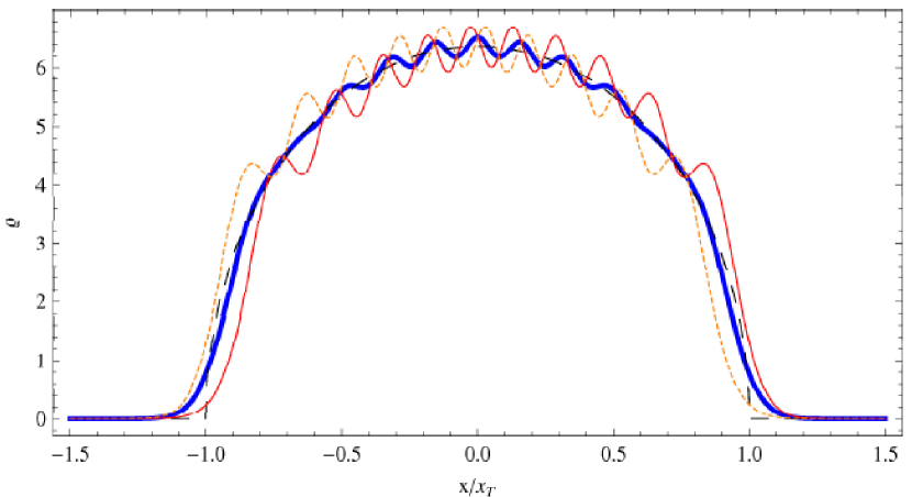
Figure 1: Plot of the time dependent particle density $\varrho(x,t)$ for 10 atoms as function of $x$ measured in units of the radius $x_{T}$. The thin solid line (red in color) is at $t=0$, the thick solid line (blue in color) is at $t=\pi/2\omega$ and the thin dotted line (orange in color) is at $t=\pi/\omega$. We plot the average density $\bar{\varrho}(x)$ for comparison as a black dashed line.

We now consider the signatures of these oscillations in the time-dependent transmission of a weak CW field $\mathcal{E}(x,t),$ which is sent through the condensate along its axis. This field is assumed to be far-detuned from a resonant transition of the atoms of the condensate, and will create a polarization density along the sample. The latter can be given as $\mathcal{P}=\mathcal{N}d^{2}\mathcal{E}/\hbar(\Delta-i\gamma)$, where $\mathcal{N}$ is the volume density of the atoms, $d$ is the dipole matrix element and $\gamma$ is the width of the transition in question, while $\Delta=\omega_{0}-\omega_{L}$ is the detuning between the resonant transition frequency $\omega_{0}$ and the carrier of the probing field $\omega_{L}$. We write $\mathcal{N=N}_{a}\varrho(x,t)$, where $\mathcal{N}_{a}$ is the average number of atoms in unit cross section. In real experiments MSKE03 ; PWM04 ; KWW04 one has a lattice of pencil shaped  samples, therefore the actual value of $\mathcal{N}_{a}$ is the inverse of the cross section of one such “pencil”. (We do not consider here the effect of light propagating between these pencils.) The polarization, $\mathcal{P}$ leads to a space and time dependent susceptibility and index of refraction

$$n(x,t)=\left(1+\frac{\mathcal{N}_{a}d^{2}}{\epsilon_{0}\hbar(\Delta-i\gamma)}\varrho(x,t)\right)^{1/2}$$ (11)

As the  time dependence of the harmonic trap is very slow with respect to the frequency of the optical fields, instead of the wave equation we shall solve the one dimensional amplitude equation for the electric field:

$$\frac{\partial^{2}}{\partial x^{2}}E(x,t)+n^{2}(x,t)k^{2}E(x,t)=0$$ (12)

where $k=2\pi/\lambda_{0}$ is the corresponding wave number in vacuum. Here $E(x,t)$ is the temporally slowly varying amplitude of the full electric field: $\mathcal{E}(x,t)=E(x,t)e^{-i\omega_{L}t}$. The solution of this equation with a given incoming plane wave from the negative $x$ direction shall yield the transmitted wave $E_{\mathrm{tr}}(t)e^{ikx}$ for $x\gg x_{T},$ as well as a reflected wave at $x\ll-x_{T}$. The results of a numerical solution will be discussed below. In order to get a better insight into the nature of the problem we also present  an approximate analytic solution to (12) by a 2nd order WKB approximation obtained for the forward propagating wave as

$$E_{\mathrm{f}}(x,t)=\frac{1}{\sqrt{n(x,t)}}E_{0}\exp\left(ik{\textstyle\int\limits_{x_{0}}^{x}}n(x^{\prime},t)dx^{\prime}-i\frac{n^{\prime}(x)}{4kn^{2}(x)}-i\int_{x_{0}}^{x}\frac{(n^{\prime}(x^{\prime}))^{2}}{8kn^{3}(x^{\prime})}dx^{\prime}\right),$$ (13)

where $E_{0}$ is the incident field amplitude at $x_{0}$, far before the condensate. The transmission coefficient of the condensate depends only on time for $x\gg x_{T}$, i.e. far beyond the condensate:

$$T(t)=\left|\frac{E_{\mathrm{f}}(x,t)}{E_{0}}\right|^{2}=\exp\left(-2k\int_{x_{0}}^{x}\operatorname{Im}n(x^{\prime},t)dx^{\prime}+\frac{1}{4k}\int_{x_{0}}^{x}\operatorname{Im}\frac{(n^{\prime}(x^{\prime}))^{2}}{n^{3}(x^{\prime})}dx^{\prime}\right)$$ (14)

since $n(x,t)=1$ for $x\gg x_{T}$. In case of an off-resonant external field we can expand the index of refraction given by (11) under the integral up to second order as

$$n(x,t)=1+\beta\varrho(x,t)/2-\beta^{2}\varrho^{2}(x,t)/8$$ (15)

with $\beta=\mathcal{N}_{a}d^{2}/(\epsilon_{0}\hbar(\Delta-i\gamma))$. In the following we consider the light source at $x_{0}=-\infty$, and a photodetector at $x=\infty$. Substituting the second order expansion of the refractive index into the formula for the transmission we have:

$$T(t)=\exp\left(-Nk\operatorname{Im}\beta+\frac{k\operatorname{Im}\beta^{2}}{4}\int_{-\infty}^{\infty}\varrho^{2}(x,t)dx+\frac{\operatorname{Im}\beta^{2}}{16k}\int_{-\infty}^{\infty}(\varrho^{\prime}(x,t))^{2}dx\right)$$ (16)

We write $\varrho(x,t)=r_{0}(x)+r_{1}(x)\cos(\omega t+\alpha)$, where $r_{0}(x)=|c_{0}|^{2}\varrho_{0}(x)+|c_{1}|^{2}\varrho_{1}(x)$ is an even function and $r_{1}(x)=2|c_{0}||c_{1}|\varrho_{01}(x)$ is an odd function of $x$, and $\alpha$ denotes the relative phase of $c_{0}$ and $c_{1}$. Substituting this into (16) and using the parity of $r_{0}$ and $r_{1}$, we obtain the following formula for the transmission:

$$T(t)=T_{N}\exp\left[\zeta\cos\left(2(\omega t+\alpha)\right)\right],$$ (17)

where

$$T_{N}=\exp\left(-Nk\operatorname{Im}\beta+\frac{k}{4}\operatorname{Im}(\beta^{2})\int_{-\infty}^{\infty}\left(r_{0}^{2}(x)+\frac{1}{2}r_{1}^{2}(x)\right)dx+\frac{\operatorname{Im}\beta^{2}}{16k}\int_{-\infty}^{\infty}\left((r_{0}^{\prime 2}+\frac{1}{2}(r_{1}^{\prime 2}\right)dx\right)$$

does not depend on time, $\alpha=\arg(c_{0}-c_{1})$, and

$$\zeta=(2|c_{0}||c_{1}|)^{2}\operatorname{Im}(\beta^{2})(kR_{1}(N)/8+R_{2}(N)/32k)$$ (18)

with the integrals

$$R_{1}(N)=\int_{-\infty}^{\infty}\varrho_{01}^{2}(x)dx,\ \ R_{2}(N)=\int_{-\infty}^{\infty}(\varrho_{01}^{\prime 2}(x))dx$$

depending only on the number of particles in the sample. $R_{1}$ and $R_{2}$ can be easily calculated up to several hundreds of atoms with a finite sum expression, which can be derived using known formulas for products of Hermite polynomials GR07 .

We can expand the time dependent factor in (17) into a Jacobi form AS65 , which is directly related to the discrete Fourier transform of the time dependent transmission:

$$T(t)=T_{N}\left[I_{0}(\zeta)+2\sum_{s=1}^{\infty}I_{s}(\zeta)\cos\left(2s(\omega t+\alpha)\right)\right]$$ (19)

where $I_{s}(\zeta)$ are the modified Bessel functions. This means that the complex Fourier coefficients $\tilde{T}$ of the time-dependent transmisson are proportional to modified Bessel functions with the same argument, $s=0,1,2,...$ :

$$\tilde{T}(2s\omega)\sim I_{s}(\zeta)e^{-2si\alpha}.$$ (20)

$I_{1}(\zeta)$ is real, therefore the phase of $\tilde{T}(2\omega)$ yields the relative phase of the states $\Psi_{0}$ and $\Psi_{1}$: $\alpha=-\frac{1}{2}\arg\tilde{T}(2\omega)$, in the case of a positive detuning. ($I_{1}$ is odd for real arguments, and the sign of $\zeta$ is the sign of $\Delta$.) A well known relation for the Bessel functions AS65 enables us to calculate $\zeta$ from the transmission spectrum:

$$\zeta=\frac{2I_{1}(\zeta)}{I_{0}(\zeta)-I_{2}(\zeta)}=\frac{2\tilde{T}(2\omega)e^{2i\alpha}}{\tilde{T}(0)-|\tilde{T}(4\omega)|}$$ (21)

Since $\zeta$ is composed of quantities which characterize the condensate and its interaction with the CW field, the knowledge of $\zeta$ gives information about these quantities. E.g. if we know everything in $\zeta$ except for the coefficients $c_{0}$ and $c_{1}$, then a measurement of the time-dependent transmission yields the value of $|c_{0}||c_{1}|$ and the relative phase $\alpha$ which (using $|c_{0}|^{2}+|c_{1}|^{2}=1$) allows us to calculate $c_{0}$ and $c_{1}$ up to a global phase factor. Alternatively, the number of particles in the condensate can be calculated from the Fourier coefficients of the time-dependent transmission, if the other quantities in $\zeta$ are already known. This means that one can accurately measure the number of particles in a condensate without destroying it.

We illustrate the use of the modulated transmission for this latter case, by processing a simulated transmisson signal which we obtain from the numerical solution of the second order amplitude equation (12). We assume a sample where ⁸⁷Rb atoms are trapped in an array of pencil shaped condensates MSKE03 ; PWM04 ; KWW04 containing 30 atoms in a superposition state (1) with $c_{0}=c_{1}=1/\sqrt{2}$. The laser light for the transmission measurement is assumed to be detuned with an angular frequency $\Delta=2\pi\times 90$ MHz from the center of the $D_{1}$ line ($\lambda_{0}=$794.978 nm), and we use $\gamma=1.80647\times 10^{7}$ 1/s and $d=1.4651\times 10^{-29}$ Cm RbData . Fig. 2 shows the density $\varrho(x,t=0)$ and the electric field amplidude $E(x,t=0)$ for 30 atoms obtained from the solution of Eq. (12). Fig. 3 shows the Fourier amplitudes of the time-dependent transmission, assuming a longitudinal trap angular frequency $\omega=2\pi\times 100$ Hz. A calculation based on the data shown in this figure and using Eqs. (18) and (21) reproduce correctly that the sample contains 30 or 31 atoms.

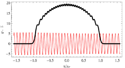
Figure 2: Plot of the electric field amplitude $E(x/x_{T},t=0)$, resulting from the numerical solution of Eq. (12), with thin solid line (red in color), in arbitrary units, as a probing field passing through the condensate of 30 atoms with particle density $\varrho(x/x_{T},t=0)$, plotted as a thick black line. The approximate analytic solution given by Eq.(13) differs from the numerical result by less then the line thickness in this figure.

Figure 3: Plot of the magnitude of the Fourier coefficients of the time dependent transmission.

In conclusion, we have constructed an exact many body superposition state for the Tonks gas, exhibiting a time-dependent particle density in a swinging mode. Generalizations for superpositions involving higher excited modes are straightforward. The model for the interaction of the Tonks gas with a weak laser beam opens the possibility of measuring the effect of these density oscillations as a weak but measurable oscillation in the transmission signal. The approximate analytic formula obtained for this time-dependent transmission allows for the calculation of the quantities which characterize the condensate and its interaction with the CW field: the coefficients of the many body superposition state, or the number of atoms in the Tonks gas could be measured without destroying the sample.

This work was supported by the Hungarian Scientific Research Fund OTKA under Contracts No. T48888, M36803, M045596. We thank P. Földi for useful discussions.

References

- (1) E.P. Gross, Il Nuovo Cimento 20 454 (1961), L.P. Pitaevskii, Soviet Physics JETP 13, 451-454 (1961).
- (2) F. Dalfovo, S. Giorgini, L. P. Pitaevskii, and S. Stringari, Rev. Mod. Phys. 71, 463 (1999).
- (3) E. B. Kolomeisky, T. J. Newman, J. P. Straley, and X. Qi, Phys. Rev. Lett. 85, 1146 (2000).
- (4) H. Moritz, T. Stöferle, M. Köhl, and T. Esslinger, Phys. Rev. Lett. 91, 250402 (2003).
- (5) K. Bongs, S. Burger, S. Dettmer, et al, Phys. Rev. A 63, 31602 (2001)
- (6) A. Minguzzi, P. Vignolo, M. L. Chiofalo, and M. P. Tosi, Phys. Rev. A 64, 033605 (2001).
- (7) C. Menotti, S. Stringari, Phys. Rev. A 66, 043610 (2002).
- (8) M. D. Girardeau, E. M. Wright, Phys. Rev. Lett. 84, 5239 (2000).
- (9) B. Paredes, A. Widera, V. Murg et al., Nature 429, 277 (2004).
- (10) T. Kinoshita,T.Wenger, D.S.Weiss, Science, 305, 1125 (2004).
- (11) L. Tonks, Phys. Rev. 50, 955 (1936).
- (12) M. D. Girardeau, J. Math. Phys. 1, 516 (1960).
- (13) E. Lieb, W. Liniger, Phys. Rev. 130, 1605 (1963).
- (14) C. J. Pethick, H. Smith, Bose-Einstein condensation in dilute gases, (Cambridge, 2008).
- (15) I. Bloch, J. Dalibard, W. Zwerger, Rev. Mod. Phys., 885 (2008).
- (16) D. S. Petrov, G. V Shlaypnikov, and J. T. M Walraven, Phys. Rev. Lett. 85, 3745 (2000).
- (17) V. Dunjko, V. Lorent, M. Olshanii, Phys. Rev. Lett. 86, 5413 (2001).
- (18) M. Olshanii, V. Dunjko, Phys. Rev. Lett. 91, 090401 (2003).
- (19) P. Pedri, L. Santos, Phys. Rev. Lett. 91, 110401 (2003).
- (20) M. D. Girardeau, E. M. Wright, J. M. Triscari, Phys. Rev. A 63, 033601 (2001).
- (21) I. S. Gradshtein, I. M. Ryzhik, Table of Integrals, Series, and products 7-th ed. (Academic Press, Amsterdam, 2007).
- (22) Handbook of Mathematical Functions, edited by M. Abramowitz and I. Stegun (Dover, New York, 1965).
- (23) Daniel A. Steck, ”Rubidium 87 D Line Data”, available online at http://steck.us/alkalidata (revision 2.1.1, 30 April 2009).