Quasi-Newton methods on Grassmannians and multilinear approximations of tensors

Abstract

In this paper we proposed quasi-Newton and limited memory quasi-Newton methods for objective functions defined on Grassmannians or a product of Grassmannians. Specifically we defined bfgs and l-bfgs updates in local and global coordinates on Grassmannians or a product of these. We proved that, when local coordinates are used, our bfgs updates on Grassmannians share the same optimality property as the usual bfgs updates on Euclidean spaces. When applied to the best multilinear rank approximation problem for general and symmetric tensors, our approach yields fast, robust, and accurate algorithms that exploit the special Grassmannian structure of the respective problems, and which work on tensors of large dimensions and arbitrarily high order. Extensive numerical experiments are included to substantiate our claims.

1 Introduction

1.1 Quasi-Newton and limited memory quasi-Newton algorithms on Grassmannians

We develop quasi-Newton and limited memory quasi-Newton algorithms for functions defined on a Grassmannian $\operatorname*{Gr}(n,r)$ as well as a product of Grassmannians $\operatorname*{Gr}(n_{1},r_{1})\times\dots\times\operatorname*{Gr}(n_{k},r_{k})$, with bfgs and l-bfgs updates. These are algorithms along the lines of the class of algorithms studied by Edelman, Arias, and Smith in [24] and more recently, the monograph of Absil, Mahony, and Sepulchre in [2]. They are algorithms that respect the Riemannian metric structure of the manifolds under consideration, and not mere applications of the usual bfgs and l-bfgs algorithms for functions on Euclidean space. The actual computations of our bfgs and l-bfgs algorithms on Grassmannians, like the algorithms in [24], require nothing more than standard numerical linear algebra routines and can therefore take advantage of the many high quality softwares developed for matrix computations [3, 40]. In other words, manifold operations such as movement along geodesics and parallel transport of tangent vectors and linear operators do not require actual numerical solutions of the differential equations defining these operations; instead they are characterized as matrix operations on local and global coordinate representations (as matrices) of points on the Grassmannians or points on an appropriate vector bundle.

A departure and improvement from existing algorithms for manifold optimization [1, 2, 24, 27] is that we undertake a local coordinates approach. This allows our computational costs to be reduced to the order of the intrinsic dimension of the manifold as opposed to the dimension of ambient Euclidean space. For a Grassmannian embedded in the Euclidean space of $n\times r$ matrices, i.e.$\ \operatorname*{Gr}(n,r)\subseteq\mathbb{R}^{n\times r}$, computations in local coordinates have $r(n-r)$ unit cost whereas computations in global coordinates, like the ones in [24], have $nr$ unit cost. This difference becomes more pronounced when we deal with products of Grassmannians $\operatorname*{Gr}(n_{1},r_{1})\times\dots\times\operatorname*{Gr}(n_{k},r_{k})\subseteq\mathbb{R}^{n_{1}\times r_{1}}\times\dots\times\mathbb{R}^{n_{k}\times r_{k}}$—for $n_{i}=O(n)$ and $r_{i}=O(r)$, we have a computational unit cost of $O(kr(n-r))$ and $O(krn)$ flops between the local and global coordinates versions the bfgs algorithms. More importantly, we will show that our bfgs update in local coordinates on a product of Grassmannians (and Grassmannian in particular) shares the same well-known optimality property of its Euclidean counterpart, namely, it is the best possible update of the current Hessian approximation that satisfies the secant equations and preserves symmetric positive definiteness (cf. Theorem 9). For completeness and as an alternative, we also provide the global coordinate version of our bfgs and l-bfgs algorithms analogous to the algorithms described in [24]. However the aforementioned optimality is not possible for bfgs in global coordinates.

While we have limited our discussions to bfgs and l-bfgs updates, it is straightforward to substitute these updates with other quasi-Newton updates (e.g. dfp or more general Broyden class updates) by applying the same principles in this paper.

1.2 Multilinear approximations of tensors and symmetric tensors

In part to illustrate the efficiency of these algorithms, this paper also addresses the following two related problems about the multilinear approximations of tensors and symmetric tensors, which are also important problems in their own right with various applications in analytical chemistry [53], bioinformatics [47], computer vision [55], machine learning [44, 41], neuroscience [45], quantum chemistry [35], signal processing [10, 13, 18], etc. See also the very comprehensive bibliography of the recent survey [38]. In data analytic applications, the multilinear approximation of general tensors is the basis behind the Tucker model [54] while the multilinear approximation of symmetric tensors is used in independent components analysis [14, 18] and principal cumulant components analysis [44, 41]. The algorithms above provide a natural method to solve these problems that exploits their unique structures.

The first problem is that of finding a best multilinear rank-$(p,q,r)$ approximation to a tensor, i.e. approximating a given tensor $\mathcal{A}\in\mathbb{R}^{l\times m\times n}$ by another tensor $\mathcal{B}\in\mathbb{R}^{l\times m\times n}$ of lower multilinear rank [31, 20],

$$\min_{\operatorname*{rank}(\mathcal{B})\leq(p,q,r)}\lVert\mathcal{A}-\mathcal{B}\rVert.$$

For concreteness we will assume that the norm in question is the Frobenius or Hilbert-Schmidt norm $\lVert\,\cdot\,\rVert_{F}$. In notations that we will soon define, we seek matrices $X,Y,Z$ with orthonormal columns and a tensor $\mathcal{C}\in\mathbb{R}^{p\times q\times r}$ such that

$$\operatorname*{argmin}_{X\in\operatorname*{O}(l,p),Y\in\operatorname*{O}(m,q),Z\in\operatorname*{O}(n,r),\mathcal{C}\in\mathbb{R}^{l\times m\times n}}\lVert\mathcal{A}-(X,Y,Z)\cdot\mathcal{C}\rVert_{F}.$$ (1)

The second problem is that of finding a best multilinear rank-$r$ approximation to a symmetric tensor $\mathcal{S}\in\mathsf{S}^{3}(\mathbb{R}^{n})$. In other words, we seek a matrix $Q$ whose columns are mutually orthonormal, and a symmetric tensor $\mathcal{C}\in\mathsf{S}^{3}(\mathbb{R}^{r})$ such that a multilinear transformation of $\mathcal{C}$ by $Q$ approximates $\mathcal{S}$ in the sense of minimizing a sum-of-squares loss. Using the same notation as in (1), the problem is

$$\operatorname*{argmin}_{Q\in\operatorname*{O}(n,r),\mathcal{C}\in\mathsf{S}^{3}(\mathbb{R}^{r})}\lVert\mathcal{S}-(Q,Q,Q)\cdot\mathcal{C}\rVert_{F}.$$ (2)

This problem is significant because many important tensors that arise in applications are symmetric tensors.

We will often refer to the first problem as the general case and the second problem as the symmetric case. Most discussions are presented for the case of $3$-tensors for notational simplicity but key expressions are given for tensors of arbitrary order to facilitate structural analysis of the problem and algorithmic implementation. The matlab codes of all algorithms in this paper are available for download at [50, 51]. All of our implementations will handle $3$-tensors and in addition, our implementation of the bfgs with scaled identity as initial Hessian approximation will handle tensors of arbitrary order. In fact the reader will find an example of a tensor of order-$10$ in Section 11, included to show that our algorithms indeed work on high-order tensors.

Our approach is summarized as follows. Observe that due to the unitary invariance of the sum-of-squares norm $\lVert\,\cdot\,\rVert_{F}$, the orthonormal matrices $U,V,W$ in (1) and the orthonormal matrix $Q$ in (2) are only determined up to an action of $\operatorname*{O}(p)\times\operatorname*{O}(q)\times\operatorname*{O}(r)$ and an action of $\operatorname*{O}(r)$, respectively. We exploit this to our advantage by reducing the problems to an optimization problem on a product of Grassmannians and a Grassmannian, respectively. Specifically, we reduce (1), a minimization problem over a product of three Stiefel manifolds and a Euclidean space $\operatorname*{O}(l,p)\times\operatorname*{O}(m,q)\times\operatorname*{O}(n,r)\times\mathbb{R}^{p\times q\times r}$, to a maximization problem over a product of three Grassmannians $\operatorname*{Gr}(l,p)\times\operatorname*{Gr}(m,q)\times\operatorname*{Gr}(n,r)$; and likewise we reduce (2) from $\operatorname*{O}(n,r)\times\mathsf{S}^{3}(\mathbb{R}^{r})$ to a maximization problem over $\operatorname*{Gr}(n,r)$. This reduction of (1) to product of Grassmannians has been exploited in [25, 34, 33]. The algorithms in [25, 34, 33] involve the Hessian, either explicitly or implicitly via its approximation on a tangent. Whichever the case, the reliance on Hessian in these methods results in them quickly becoming infeasible as the size of the problem increases. With this in mind, we consider the quasi-Newton and limited memory quasi-Newton approaches described in the first paragraph of this section.

An important case not addressed in [25, 34, 33] is the multilinear approximation of symmetric tensors (2). Note that the general (1) and symmetric (2) cases are related but different, not unlike the way the singular value problem differs from the symmetric eigenvalue problem for matrices. The problem (1) for general tensors is linear in the entries of $U,V,W$ (quadratic upon taking norm-squared) whereas the problem (2) for symmetric tensors is cubic in the entries of $Q$ (sextic upon taking norm-squared). To the best of our knowledge, all existing solvers for (2) are unsatisfactory because they rely on algorithms for (1). A typical heuristic is as follows: find three orthonormal matrices $Q_{1},Q_{2},Q_{3}$ and a nonsymmetric $\mathcal{C}^{\prime}\in\mathbb{R}^{r\times r\times r}$ that approximates $\mathcal{S}$,

$$\mathcal{S}\approx(Q_{1},Q_{2},Q_{3})\cdot\mathcal{C}^{\prime},$$

then artificially set $Q_{1}=Q_{2}=Q_{3}=Q$ by either averaging or choosing the last iterate and then symmetrize $\mathcal{C}^{\prime}$. This of course is not ideal. Furthermore, using the framework developed for the general tensor approximation to solve the symmetric tensor approximation problem will be computationally much more expensive. In particular, to optimize $\mathcal{S}\approx(Q_{1},Q_{2},Q_{3})\cdot\mathcal{C}^{\prime}$ without taking the symmetry into account incurs a $k$-fold increase in computational cost relative to $\mathcal{S}\approx(Q,\dots,Q)\cdot\mathcal{C}$. The algorithm proposed in this paper solves (2) directly. It finds a single $Q\in\operatorname*{O}(n,r)$ and a symmetric $\mathcal{C}\in\mathsf{S}^{3}(\mathbb{R}^{r})$ with

$$\mathcal{S}\approx(Q,Q,Q)\cdot\mathcal{C}.$$

The symmetric case can often be more important than the general case, not surprising since symmetric tensors are common in practice, arising as higher order derivatives of smooth multivariate real-valued functions, higher order moments and cumulants of a vector-valued random variable, etc.

Like the Grassmann-Newton algorithms in [25, 34] and the trust-region approach in [33, 32], the quasi-Newton algorithms proposed in this article have guaranteed convergence to stationary points and represent an improvement over Gauss-Seidel type coordinate-cycling heuristics like alternating least squares (als), higher-order orthogonal iteration (hooi), or higher-order singular value decomposition (hosvd) [14]. And as far as accuracy is concerned, our algorithms perform as well as the algorithms in [25, 32, 34] and outperform Gauss-Seidel type strategies in many cases. As far as robustness and speed are concerned, our algorithms work on much larger problems and perform vastly faster than Grassmann-Newton algorithm. Asymptotically the memory storage requirements of our algorithms are of the same order-of-magnitude as Gauss-Seidel type strategies. For large problems, our Grassmann l-bfgs algorithm outperforms even Gauss-Seidel strategies (in this case hooi), which is not unexpected since it has the advantage of requiring only a small number of prior iterates.

We will give the reader a rough idea of the performance of our algorithms. Using matlab on a laptop computer, we attempted to find a solution to an accuracy within machine precision, i.e. $\approx 10^{-13}$. For general $3$-tensors of size $200\times 200\times 200$, our Grassmann l-bfgs algorithm took less than $13$ minutes while for general $4$-tensors of size $50\times 50\times 50\times 50$, it took about $7$ minutes. For symmetric $3$-tensors of size $200\times 200\times 200$, our Grassmann bfgs algorithm took about $5$ minutes while for symmetric $4$-tensors of size $50\times 50\times 50\times 50$, it took less than $2$ minutes. In all cases, we seek a rank-$(5,5,5)$ or rank-$(5,5,5,5)$ approximation. For a general order-$10$ tensor of dimensions $5\times\dots\times 5$, a rank-$(2,\dots,2)$ approximation took about $15$ minutes to reach the same accuracy as above. More extensive numerical experiments are reported in Section 11. The reader is welcomed to try our algorithms, which have been made publicly available at [50, 51].

1.3 Outline

The structure of the article is as follows. In Sections 2 and 3, we present a more careful discussion of tensors, symmetric tensors, multilinear rank, and their corresponding multilinear approximation problems. In Section 4 we will discuss how quasi-Newton methods in Euclidean space may be extended to Riemannian manifolds and, in particular, Grassmannians. Section 5 contains a discussion on geodesic curves and transport of vectors on Grassmannians. In Section 6 we present the modifications on quasi-Newton methods with bfgs updates in order for them to be well-defined on Grassmannians. Also, the reader will find proof of the optimality properties of bfgs updates on products of Grassmannians. Section 7 gives the corresponding modifications for limited memory bfgs updates. Section 8 states the corresponding expressions for the tensor approximation problem, which are defined on a product of Grassmannians. The symmetric case is detailed in section 9. Section 10 contains a few examples with numerical calculations illustrating the presented concepts. The implementation and the experimental results are found in Section 11. Related work and the conclusions are discussed in Section 12 and 13 respectively.

1.4 Notations

Tensors will be denoted by calligraphic letters, e.g. $\mathcal{A}$, $\mathcal{B}$, $\mathcal{C}$. Matrices will be denoted in upper case letters, e.g. $X$, $Y$, $Z$. We will also use upper case letters $X$, $X_{k}$ to denote iterates or elements of a Grassmannian since we represent them as (equivalence classes of) matrices with orthonormal columns. Vectors and iterates in vector form are denoted with lower case letters, e.g. $x$, $y$, $x_{k}$, $y_{k}$, where the subscript is the iteration index. To denote scalars we use lower case Greek letters, e.g. $\alpha$, $\beta$, and $t$, $t_{k}$.

We will use the usual symbol $\mathbin{\scalebox{0.88}{$\displaystyle\otimes$}}$ to denote the outer product of tensors and a large boldfaced version $\mathbin{\scalebox{1.12}{$\displaystyle\varotimes$}}$ to denote the Kronecker product of operators. For example, if $A\in\mathbb{R}^{m\times n}$ and $B\in\mathbb{R}^{p\times q}$ are matrices, then $A\mathbin{\scalebox{0.88}{$\displaystyle\otimes$}}B$ will be a $4$-tensor in $\mathbb{R}^{m\times n\times p\times q}$ whereas $A\mathbin{\scalebox{1.12}{$\displaystyle\varotimes$}}B$ will be a matrix in $\mathbb{R}^{mp\times nq}$. In the former case, we regard $A$ and $B$ as $2$-tensors while in the latter case, we regard them as matrix representations of linear operators. The contracted products used in this paper are defined in Appendix A.

For $r\leq n$, we will let $\operatorname*{O}(n,r)=\{X\in\mathbb{R}^{n\times r}\mid X^{\mathsf{T}}X=I\}$ denote the Stiefel manifold of $n\times r$ matrices with orthonormal columns. The special case $r=n$, i.e. the orthogonal group, will be denoted $\operatorname*{O}(n)$. For $r\leq n$, $\operatorname*{O}(r)$ acts on $\operatorname*{O}(n,r)$ via right multiplication. The set of orbit classes $\operatorname*{O}(n,r)/\operatorname*{O}(r)$ is a manifold called the Grassmann manifold or Grassmannian (we adopt the latter name throughout this article) and will be denoted $\operatorname*{Gr}(n,r)$.

In this paper, we will only cover a minimal number of notions and notations required to describe our algorithm. Further mathematical details concerning tensors, tensor ranks, tensor approximations, as well as the counterpart for symmetric tensors may be found in [8, 20, 25]. Specifically we will use the notational and analytical framework for tensor manipulations introduced in [25, Section 2] and assume that these concepts are familiar to the reader.

2 General and symmetric tensors

Let $V_{1},\dots,V_{k}$ be real vector spaces of dimensions $n_{1},\dots,n_{k}$ respectively and let $\mathbf{A}$ be an element of the tensor product $V_{1}\mathbin{\scalebox{0.88}{$\displaystyle\otimes$}}\dots\mathbin{\scalebox{0.88}{$\displaystyle\otimes$}}V_{k}$, i.e. $\mathbf{A}$ is a tensor of order $k$ [30, 39, 56]. Up to a choice of bases on $V_{1},\dots,V_{k}$, one may represent a tensor $\mathbf{A}$ as a $k$-dimensional hypermatrix $\mathcal{A}=[a_{i_{1}\cdots i_{k}}]\in\mathbb{R}^{n_{1}\times\dots\times n_{k}}$. Similarly, let $V$ be a real vector space of dimension $n$ and $\mathbf{S}\in\mathsf{S}^{k}(V)$ be a symmetric tensor of order $k$ [30, 39, 56]. Up to a choice of basis on $V$, $\mathbf{S}$ may be represented as a $k$-dimensional hypermatrix $\mathcal{S}=[s_{i_{1}\cdots i_{k}}]\in\mathbb{R}^{n\times\dots\times n}$ whose entries are invariant under any permutation of indices, i.e.

$$s_{i_{\sigma(1)}\cdots i_{\sigma(k)}}=s_{i_{1}\cdots i_{k}}\qquad\text{for every }\sigma\in\mathfrak{S}_{k}$$ (3)

We will write $\mathsf{S}^{k}(\mathbb{R}^{n})$ for the subspace of $\mathbb{R}^{n\times\dots\times n}$ satisfying (3). Henceforth, we will assume that there are some predetermined bases and will not distinguish between a tensor $\mathbf{A}\in V_{1}\mathbin{\scalebox{0.88}{$\displaystyle\otimes$}}\dots\mathbin{\scalebox{0.88}{$\displaystyle\otimes$}}V_{k}$ and its hypermatrix representation $\mathcal{A}\in\mathbb{R}^{n_{1}\times\dots\times n_{k}}$ and likewise for a symmetric tensor $\mathbf{S}\in\mathsf{S}^{k}(V)$ and its hypermatrix representation $\mathcal{S}\in\mathsf{S}^{k}(\mathbb{R}^{n})$. Furthermore we will sometimes present our discussions for the case $k=3$ for notational simplicity. We often call an order-$k$ tensor simply as a $k$-tensor and an order-$k$ symmetric tensor as a symmetric $k$-tensor.

As we have mentioned in Section 1, symmetric tensors are common in applications, largely because of the two examples below. The use of higher-order statistics in signal processing and neuroscience, most notably the technique of independent component analysis, symmetric tensors often play a central role. The reader is referred to [8] for further discussion of symmetric tensors.

Example 1.

Let $m\in\{1,2,\dots,\infty\}$ and $\Omega\subseteq\mathbb{R}^{n}$ be an open subset. If $f\in C^{m}(\Omega)$, then for $k=1,\dots,m$, the $k$th derivative of $f$ at $\mathbf{a}\in\Omega$ is a symmetric tensor of order $k$,

$$D^{k}f(\mathbf{a})=\left[\frac{\partial^{k}f}{\partial x_{1}^{i_{1}}\dots\partial x_{n}^{i_{n}}}(\mathbf{a})\right]_{i_{1}+\dots+i_{n}=k}\in\mathsf{S}^{k}(\mathbb{R}^{n}).$$

For $k=1,2$, the vector $D^{1}f(\mathbf{a})$ and the matrix $D^{2}f(\mathbf{a})$ are the gradient and Hessian of $f$ at $\mathbf{a}$, respectively.

Example 2.

Let $X_{1},\dots,X_{n}$ be random variables with respect to the same probability distribution $\mu$. The moments and cumulants of the random vector $\mathbf{X}=(X_{1},\dots,X_{n})$ are symmetric tensors of order $k$ defined by

$$m_{k}(\mathbf{X)} =\bigl{[}E(x_{i_{1}}x_{i_{2}}\cdots x_{i_{k}})\bigr{]}_{i_{1},\dots,i_{k}=1}^{n}$$

$$=\left[\idotsint x_{i_{1}}x_{i_{2}}\cdots x_{i_{k}}~{}d\mu(x_{i_{1}})\cdots d\mu(x_{i_{k}})\right]_{i_{1},\dots,i_{k}=1}^{n}$$

and

$$\kappa_{k}(\mathbf{X})=\left[\sum\nolimits_{\begin{subarray}{c}A_{1}\sqcup\dots\sqcup A_{p}\\ =\{i_{1},\dots,i_{k}\}\end{subarray}}(-1)^{p-1}(p-1)!E({\textstyle\prod\nolimits_{i\in A_{1}}}x_{i})\cdots E({\textstyle\prod\nolimits_{i\in A_{p}}}x_{i})\right]_{i_{1},\dots,i_{k}=1}^{n}$$

respectively. The sum above is taken over all possible partitions $\{i_{1},\dots,i_{k}\}=A_{1}\sqcup\dots\sqcup A_{p}$. It is not hard to show that both $m_{k}(\mathbf{X)}$ and $\kappa_{k}(\mathbf{X)}\in\mathsf{S}^{k}(\mathbb{R}^{n})$. For $n=1$, the quantities $\kappa_{k}(\mathbf{X})$ for $k=1,2,3,4$ have well-known names: they are the expectation, variance, skewness, and kurtosis of the random variable $X$, respectively.

3 Multilinear transformation and multilinear rank

Matrices can act on other matrices through two independent multiplication operations: left-multiplication and right-multiplication. If $C\in\mathbb{R}^{p\times q}$ and $X\in\mathbb{R}^{m\times p}$, $Y\in\mathbb{R}^{n\times q}$, then the matrix $C$ may be transformed into the matrix $A\in\mathbb{R}^{m\times n}$, by

$$A=XCY^{\mathsf{T}},\qquad a_{ij}=\sum_{\alpha=1}^{p}\sum_{\beta=1}^{q}x_{i\alpha}y_{j\beta}c_{\alpha\beta}\,.$$ (4)

Matrices act on order-$3$ tensors via three different multiplication operations. As in the matrix case, these can be combined into a single formula. If $\mathcal{C}\in\mathbb{R}^{p\times q\times r}$ and $X\in\mathbb{R}^{l\times p}$, $Y\in\mathbb{R}^{m\times q}$, $Z\in\mathbb{R}^{n\times r}$, then the $3$-tensor $\mathcal{C}$ may be transformed into the $3$-tensor $\mathcal{A}\in\mathbb{R}^{l\times m\times n}$ via

$$a_{ijk}=\sum_{\alpha=1}^{p}\sum_{\beta=1}^{q}\sum_{\gamma=1}^{r}x_{i\alpha}y_{j\beta}z_{k\gamma}c_{\alpha\beta\gamma}\,.$$ (5)

We call this operation the trilinear multiplication of $\mathcal{A}$ by matrices $X$, $Y$ and $Z$, which we write succinctly as

$$\mathcal{A}=(X,Y,Z)\cdot{\mathcal{C}}.$$ (6)

This is nothing more than the trilinear equivalent of (4), which in this notation has the form

$$A=XCY^{\mathsf{T}}=(X,Y)\cdot{C}.$$

Informally, (5) amounts to multiplying the $3$-tensor $\mathcal{A}$ on its three ‘sides’ or modes by the matrices $X$, $Y$, and $Z$ respectively.

An alternative but equivalent way of writing (5) is as follows. Define the outer product of vectors $x\in\mathbb{R}^{l}$, $y\in\mathbb{R}^{m}$, $z\in\mathbb{R}^{n}$ by

$$x\mathbin{\scalebox{0.88}{$\displaystyle\otimes$}}y\mathbin{\scalebox{0.88}{$\displaystyle\otimes$}}z=[x_{i}y_{j}z_{k}]\in\mathbb{R}^{l\times m\times n},$$

and call a tensor of the form $x\mathbin{\scalebox{0.88}{$\displaystyle\otimes$}}y\mathbin{\scalebox{0.88}{$\displaystyle\otimes$}}z$ a decomposable tensor or, if non-zero, a rank-$1$ tensor. One may also view (5) as a trilinear combination (as opposed to a linear combination) of the decomposable tensors given by

$$\mathcal{A}=\sum_{\alpha=1}^{p}\sum_{\beta=1}^{q}\sum_{\gamma=1}^{r}c_{\alpha\beta\gamma}x_{\alpha}\mathbin{\scalebox{0.88}{$\displaystyle\otimes$}}y_{\beta}\mathbin{\scalebox{0.88}{$\displaystyle\otimes$}}z_{\gamma}.$$ (7)

The vectors $x_{1},\dots,x_{p}\in\mathbb{R}^{l}$, $y_{1},\dots,y_{q}\in\mathbb{R}^{m}$, $z_{1},\dots,z_{r}\in\mathbb{R}^{n}$ are, of course, the column vectors of the respective matrices $X,Y,Z$ above. In this article, we find it more natural to present our algorithms in the form (6) and therefore we refrain from using (7).

More abstractly, given linear transformations of real vector spaces $T_{u}:U\rightarrow U^{\prime}$, $T_{v}:V\rightarrow V^{\prime}$, $T_{w}:W\rightarrow W^{\prime}$, the functoriality of tensor product [30, 39] (denoted by the usual notation $\mathbin{\scalebox{0.88}{$\displaystyle\otimes$}}$ below) implies that one has an induced linear transformation between the tensor product of the respective vector spaces

$$T_{u}\mathbin{\scalebox{0.88}{$\displaystyle\otimes$}}T_{v}\mathbin{\scalebox{0.88}{$\displaystyle\otimes$}}T_{w}:U\mathbin{\scalebox{0.88}{$\displaystyle\otimes$}}V\mathbin{\scalebox{0.88}{$\displaystyle\otimes$}}W\rightarrow U^{\prime}\mathbin{\scalebox{0.88}{$\displaystyle\otimes$}}V^{\prime}\mathbin{\scalebox{0.88}{$\displaystyle\otimes$}}W^{\prime}.$$

The trilinear matrix multiplication above is a coordinatized version of this abstract transformation. In the special case where $U=U^{\prime}$, $V=V^{\prime}$, $W=W^{\prime}$ and $T_{u}$, $T_{v}$, $T_{w}$ are (invertible) change-of-basis transformations, the operation in (5) describes the manner a (contravariant) $3$-tensor transforms under change-of-coordinates of $U$, $V$ and $W$.

Associated with the trilinear matrix multiplication (6) is the following notion of tensor rank that generalizes the row-rank and column-rank of a matrix. Let $\mathcal{A}\in\mathbb{R}^{l\times m\times n}$. For fixed values of $j\in\{1,\dots,m\}$ and $k\in\{1,\dots,n\}$, consider the column vector, written in a matlab-like notation, $\mathcal{A}(:,j,k)\in\mathbb{R}^{l}$. Likewise we may consider $\mathcal{A}(i,:,k)\in\mathbb{R}^{m}$ for fixed values of $i,k$, and $\mathcal{A}(i,j,:)\in\mathbb{R}^{n}$ for fixed values of $i,j$. Define

$$r_{1}(\mathcal{A}) :=\dim(\operatorname{span}\{\mathcal{A}(:,j,k)\mid 1\leq j\leq m,1\leq k\leq n\}),$$

$$r_{2}(\mathcal{A}) :=\dim(\operatorname{span}\{\mathcal{A}(i,:,k)\mid 1\leq i\leq l,1\leq k\leq n\}),$$

$$r_{3}(\mathcal{A}) :=\dim(\operatorname{span}\{\mathcal{A}(i,j,:)\mid 1\leq i\leq l,1\leq j\leq m\}).$$

Note that $\mathbb{R}^{l\times m\times n}$ may also be viewed as $\mathbb{R}^{l\times mn}$. Then $r_{1}(\mathcal{A})$ is simply the rank of $\mathcal{A}$ regarded as an $l\times mn$ matrix, see the discussion on tensor matricization in [25] with similar interpretations for $r_{2}(\mathcal{A})$ and $r_{3}(\mathcal{A})$. The multilinear rank of $\mathcal{A}$ is the $3$-tuple $(r_{1}(\mathcal{A}),r_{2}(\mathcal{A}),r_{3}(\mathcal{A}))$ and we write

$$\operatorname*{rank}(\mathcal{A})=(r_{1}(\mathcal{A}),r_{2}(\mathcal{A}),r_{3}(\mathcal{A})).$$

We need to ‘store’ all three numbers as $r_{1}(\mathcal{A})\neq r_{2}(\mathcal{A})\neq r_{3}(\mathcal{A})$ in general—a clear departure from the case of matrices where row-rank and column-rank are always equal. Note that a rank-$1$ tensor must necessarily have multilinear rank $(1,1,1)$, i.e.$\ \operatorname*{rank}(x\mathbin{\scalebox{0.88}{$\displaystyle\otimes$}}y\mathbin{\scalebox{0.88}{$\displaystyle\otimes$}}z)=(1,1,1)$ if $x,y,z$ are non-zero vectors.

For symmetric tensors, one would be interested in transformation that preserves the symmetry. For a symmetric matrix $C\in\mathsf{S}^{2}(\mathbb{R}^{n})$, this would be

$$S=XCX^{\mathsf{T}},\qquad s_{ij}=\sum_{\alpha=1}^{r}\sum_{\beta=1}^{r}x_{i\alpha}x_{j\beta}c_{\alpha\beta}\,.$$ (8)

Matrices act on symmetric order-$3$ tensors $\mathcal{S}\in\mathsf{S}^{3}(\mathbb{R}^{n})$ via the symmetric version of (10)

$$s_{ijk}=\sum_{\alpha=1}^{r}\sum_{\beta=1}^{r}\sum_{\gamma=1}^{r}x_{i\alpha}x_{j\beta}x_{k\gamma}c_{\alpha\beta\gamma}\,.$$ (9)

We call this operation the symmetric trilinear multiplication of $\mathcal{S}$ by matrix $X$, which in the notation above, is written as

$$\mathcal{S}=(X,X,X)\cdot{\mathcal{C}}.$$

This is nothing more than the cubic equivalent of (8), which in this notation becomes

$$S=XCX^{\mathsf{T}}=(X,X)\cdot{C}.$$

Informally, (9) amounts to multiplying the $3$-tensor $\mathcal{A}$ on its three ‘sides’ or modes by the same matrix $X$. In the multilinear combination form, this is

$$\mathcal{S}=\sum_{\alpha=1}^{r}\sum_{\beta=1}^{r}\sum_{\gamma=1}^{r}c_{\alpha\beta\gamma}x_{\alpha}\mathbin{\scalebox{0.88}{$\displaystyle\otimes$}}x_{\beta}\mathbin{\scalebox{0.88}{$\displaystyle\otimes$}}x_{\gamma}$$

where the vectors $x_{1},\dots,x_{r}\in\mathbb{R}^{n}$ are the column vectors of the matrix $X$ above.

More abstractly, given a linear transformation of real vector spaces $T:V\rightarrow V^{\prime}$, the functoriality of symmetric tensor product [30, 39] implies that one has an induced linear transformation between the tensor product of the respective vector spaces

$$\mathsf{S}^{k}(T):\mathsf{S}^{k}(V)\rightarrow\mathsf{S}^{k}(V^{\prime}).$$

The symmetric trilinear matrix multiplication above is a coordinatized version of this abstract transformation. In the special case where $V=V^{\prime}$ and $T$ is an (invertible) change-of-basis transformation, the operation in (9) describes the manner a symmetric $3$-tensor transforms under change-of-coordinates of $V$.

For a symmetric tensor $\mathcal{S}\in\mathsf{S}^{3}(\mathbb{R}^{n})$, we must have

$$r_{1}(\mathcal{S})=r_{2}(\mathcal{S})=r_{3}(\mathcal{S})$$

by its symmetry. See Lemma 11 for a short proof. The symmetric multilinear rank of $\mathcal{S}$ is the common value, denoted $r_{\mathsf{S}}(\mathcal{S})$. When referring to a symmetric tensor in this article, rank would always mean symmetric multilinear rank; e.g. a rank-$s$ symmetric tensor $\mathcal{S}$ would be one with $r_{\mathsf{S}}(\mathcal{S})=s$.

We note that there is a different notion of tensor rank and symmetric tensor rank, defined as the number of terms in a minimal decomposition of a tensor (resp. symmetric tensor) into rank-$1$ tensors (resp. rank-$1$ symmetric tensors). Associated with this notion of rank are low-rank approximation problems for tensors and symmetric tensors analogous to the ones discussed in this paper. Unfortunately, these are ill-posed problems that may not even have a solution [8, 20]. As such, we will not discuss this other notion of tensor rank. It is implicitly assumed that whenever we discuss tensor rank or symmetric tensor rank, it is with the multilinear rank or symmetric multilinear rank defined above in mind.

3.1 Multilinear approximation as maximization over Grassmannians

Let $\mathcal{A}\in\mathbb{R}^{l\times m\times n}$ be a given third order tensor and consider the problem

$$\min\{\lVert\mathcal{A}-\mathcal{B}\rVert_{F}\mid\operatorname*{rank}(\mathcal{B})\leq(p,q,r)\}.$$

Under this rank constraint, we can write $\mathcal{B}$ in factorized form

$$\mathcal{B}=(X,Y,Z)\cdot{\mathcal{C}},\quad b_{ijk}=\sum_{\alpha=1}^{p}\sum_{\beta=1}^{q}\sum_{\gamma=1}^{r}x_{i\alpha}y_{j\beta}z_{k\gamma}c_{\alpha\beta\gamma},$$ (10)

where $\mathcal{C}\in\mathbb{R}^{p\times q\times r}$ and $X\in\mathbb{R}^{l\times p}$, $Y\in\mathbb{R}^{m\times q}$, $Z\in\mathbb{R}^{n\times r}$, are full rank matrices. In other words, one would like to solve the following best multilinear rank approximation problem,

$$\min_{X,Y,Z,\mathcal{C}}\lVert\mathcal{A}-(X,Y,Z)\cdot{\mathcal{C}}\rVert_{F}.$$ (11)

This is the optimization problem underlying the Tucker model [54] that originated in psychometrics but has become increasingly popular in other areas of data analysis. In fact, there is no loss of generality if we assume $X^{\mathsf{T}}X=I$, $Y^{\mathsf{T}}Y=I$ and $Z^{\mathsf{T}}Z=I$. This is verified as follows, for any full column-rank matrices $\widetilde{X}$, $\widetilde{Y}$ and $\widetilde{Z}$ we can compute their qr-factorizations

$$\widetilde{X}=XR_{X},\quad\widetilde{Y}=YR_{Y},\quad\widetilde{Z}=ZR_{Z}$$

and multiply the right triangular matrices into the core tensor, i.e.

$$\lVert\mathcal{A}-(\widetilde{X},\widetilde{Y},\widetilde{Z})\cdot{\widetilde{\mathcal{C}}\rVert_{F}}=\lVert\mathcal{A}-(X,Y,Z)\cdot{\mathcal{C}}\rVert_{F}\quad\text{where}\quad\mathcal{C}=(R_{X},R_{Y},R_{Z})\cdot{\widetilde{\mathcal{C}}}\,.$$

With the orthonormal constraints on $X$ ,$Y$ and $Z$ the tensor approximation problem can be viewed as an optimization problem on a product of Stiefel manifolds. Using the identity

$$(U^{\mathsf{T}},V^{\mathsf{T}},W^{\mathsf{T}})\cdot\mathcal{A}\equiv{\mathcal{A}}\cdot(U,V,W),$$

we can rewrite the tensor approximation problem as a maximization problem with the objective function

$$\Phi(X,Y,Z)=\frac{1}{2}\left\|\mathcal{A}\cdot(X,Y,Z)\right\|_{F}^{2}\quad\text{s.t.}\quad X^{\mathsf{T}}X=I,\quad Y^{\mathsf{T}}Y=I,\quad Z^{\mathsf{T}}Z=I,$$ (12)

in which the small core tensor $\mathcal{C}$ is no longer present. See references [16, 25] for the elimination of $\mathcal{C}$. The objective function $\Phi(X,Y,Z)$ is invariant under orthogonal transformation of the variable matrices $X,Y,Z$ from the right. Specifically, for any orthogonal matrices $Q_{1}\in\operatorname*{O}(p)$, $Q_{2}\in\operatorname*{O}(q)$ and $Q_{3}\in\operatorname*{O}(r)$ it holds that $\Phi(X,Y,Z)=\Phi(XQ_{1},YQ_{2},ZQ_{3})$. This homogeneity property implies that $\Phi(X,Y,Z)$ is in fact defined on a product of three Grassmannians $\operatorname*{Gr}(l,p)\times\operatorname*{Gr}(m,q)\times\operatorname*{Gr}(n,r)$.

Let $\mathcal{S}\in\mathsf{S}^{3}(\mathbb{R}^{n})$ be a given symmetric $3$-tensor and consider the problem

$$\min\{\lVert\mathcal{S}-\mathcal{T}\rVert_{F}\mid\mathcal{T}\in\mathsf{S}^{3}(\mathbb{R}^{n}),\;r_{\mathsf{S}}(\mathcal{S})\leq r\}.$$

Under this rank constraint, we can write $\mathcal{T}$ in factorized form

$$\mathcal{T}=(X,X,X)\cdot{\mathcal{C}},\quad t_{ijk}=\sum_{\alpha=1}^{r}\sum_{\beta=1}^{r}\sum_{\gamma=1}^{r}x_{i\alpha}x_{j\beta}x_{k\gamma}c_{\alpha\beta\gamma},$$

where $\mathcal{C}\in\mathsf{S}^{3}(\mathbb{R}^{r})$ and $X\in\mathbb{R}^{n\times r}$ is a full-rank matrix. In other words, one would like to solve the following best symmetric multilinear rank approximation problem,

$$\min\{\lVert\mathcal{A}-(X,X,X)\cdot{\mathcal{C}}\rVert_{F}\mid X\in\operatorname*{O}(n,r),\;\mathcal{C}\in\mathsf{S}^{3}(\mathbb{R}^{r})\}.$$

As with the general case, there is no loss of generality if we assume $X^{\mathsf{T}}X=I$. With the orthonormal constraints on $X$, the tensor approximation problem can be viewed as an optimization problem on a single Stiefel manifold (as opposed to a product of Stiefel manifolds in (12)). Using the identity

$$(V^{\mathsf{T}},V^{\mathsf{T}},V^{\mathsf{T}})\cdot\mathcal{S}\equiv{\mathcal{S}}\cdot(V,V,V),$$

we may again rewrite the tensor approximation problem as a maximization problem with the objective function

$$\Phi(X)=\frac{1}{2}\left\|\mathcal{S}\cdot(X,X,X)\right\|_{F}^{2}\quad\text{s.t.}\quad X^{\mathsf{T}}X=I,$$

in which the core-tensor $\mathcal{C}$ is no longer present. As with the general case, the objective function $\Phi(X)$ also has an invariance property, namely $\Phi(X)=\Phi(XQ)$ for any orthogonal $Q\in\operatorname*{O}(r)$. As before, this homogeneity property implies that $\Phi(X)$ is well-defined on a single Grassmannian $\operatorname*{Gr}(n,r)$.

These multilinear approximation problems may be viewed as ‘dimension reduction’ or ‘rank reduction’ for tensors and symmetric tensors respectively. In general, a matrix requires $O(n^{2})$ storage and an order-$k$ tensor requires $O(n^{k})$ storage. While it is sometimes important to perform dimension reduction to a matrix, a dimension reduction is almost always necessary if one wants to work effectively with a tensor of higher order. A dimension reduction of a matrix $A\in\mathbb{R}^{n\times n}$ of the form $A\approx UCV^{\mathsf{T}}$, where $U,V\in\operatorname*{O}(n,r)$ and diagonal $C\in\mathbb{R}^{r\times r}$ reduces dimension from $O(n^{2})$ to $O(nr+r)$. A dimension reduction of a tensor $\mathcal{A}\in\mathbb{R}^{n\times\dots\times n}$ of the form $\mathcal{A}\approx(Q_{1},\dots,Q_{k})\cdot\mathcal{C}$ where $Q_{1},\dots,Q_{k}\in\operatorname*{O}(n,r)$ and $\mathcal{C}\in\mathbb{R}^{r\times\dots\times r}$, reduces dimension from $O(n^{k})$ to $O(knr+r^{k})$. If $r$ is significantly smaller than $n$, e.g. $r=O(n^{1/k})$, then a dimension reduction in the higher order case could reduce problem size by orders of magnitude.

4 Optimization in Euclidean space and on Riemannian manifolds

In this section we discuss the necessary modifications for generalizing an optimization algorithm from Euclidean space to Riemannian manifolds. Specifically we consider the quasi-Newton methods with bfgs and limited memory bfgs (l-bfgs) updates. First we state the expressions in Euclidean space and then we point out what needs to be modified. The convergence properties of quasi-Newton methods defined on manifolds were established by Gabay [27]. Numerical treatment of algorithms on the Grassmannian are given in [24, 1, 52, 42, 32]. A recent book on optimization on manifolds is [2]. In this and the next three sections, i.e. Sections 4 through 7, we will discuss our algorithms in the context of minimization problems, as is conventional. It will of course be trivial to modify them for maximization problem. Indeed the tensor approximation problems discussed in Sections 8 through 11 will all be solved as maximization problems on Grassmannians or product of Grassmannians.

4.1 BFGS updates in Euclidean Space

Assume that we want to minimize a nonlinear real valued function $f(x)$ where $x\in\mathbb{R}^{n}$. As is well-known, in quasi-Newton methods, one solves

$$H_{k}p_{k}=-g_{k},$$ (13)

to obtain the direction of descent $p_{k}$ from the current iterate $x_{k}$ and the gradient $g_{k}=\nabla f(x_{k})$ at $x_{k}$. Unlike Newton method, which uses the exact Hessian for $H_{k}$, in (13) $H_{k}$ is only an approximation of the Hessian at $x_{k}$. After computing the (search) direction $p_{k}$ one obtains the next iterate as $x_{k+1}=x_{k}+t_{k}p_{k}$ in which the step length $t_{k}$ is usually given by a line search method satisfying the Wolfe or the Goldstein conditions [46]. Instead of recomputing the Hessian at each new iterate $x_{k+1}$, it is updated from the previous approximation. The bfgs update has the following form,

$$H_{k+1}=H_{k}-\frac{H_{k}s_{k}s_{k}^{\mathsf{T}}H_{k}}{s_{k}^{\mathsf{T}}H_{k}s_{k}}+\frac{y_{k}y_{k}^{\mathsf{T}}}{y_{k}^{\mathsf{T}}s_{k}},$$ (14)

where

$$s_{k} =x_{k+1}-x_{k}=t_{k}p_{k},$$ (15)

$$y_{k} =g_{k+1}-g_{k}.$$ (16)

Quasi-Newton methods with bfgs updates are considered to be the most computationally efficient algorithms for minimization of general nonlinear functions. This efficiency is obtained by computing a new Hessian approximation as a rank-$2$ modification of the previous Hessian. The convergence of quasi-Newton methods is super-linear in a vicinity of a local minimum. In most cases the quadratic convergence of the Newton method is outperformed by quasi-Newton methods since each iteration is computationally much cheaper than a Newton iteration. A thorough study of quasi-Newton methods may be found in [46, 23]. The reader is reminded that quasi-Newton methods do not necessarily converge to local minima but only to stationary points. Nevertheless, using the Hessians that we derived in Sections 8.1 and 9.3 (for the general and symmetric cases respectively), the nature of these stationary points can often be determined.

4.2 Quasi-Newton methods on a Riemannian manifold

We will give a very brief overview of Riemannian geometry tailored specifically to our needs in this paper. First we sketch the modifications that are needed in order for an optimization algorithm to be well-defined when the objective function is defined on a manifold. For details and proof, the reader should refer to standard literature on differential and Riemannian geometry [11, 5, 2]. Informally a manifold, denoted with $M$, is an object locally homeomorphic to $\mathbb{R}^{n}$. We will regard $M$ as a submanifold of some high-dimensional ambient Euclidean space $\mathbb{R}^{N}$. Our objective function $f:M\rightarrow\mathbb{R}$ will be assumed to have (at least) continuous second order partial derivatives. We will write $f(x)$, $g(x)$, and $H(x)$ for the value of the function, the gradient, and the Hessian at $x\in M$. These will be reviewed in greater detail in the following.

Equations (13)–(16) are the basis of any algorithmic implementation involving bfgs or l-bfgs updates. The key operations are (1) computation of the gradient, (2) computation of the Hessian or its approximation, (3) subtraction of iterates, e.g. to get $s_{k}$ or $x_{k+1}$ and (4) subtraction of gradients. Each of these points needs to be modified in order for these operations to be well-defined on manifolds.

Computation of the gradient

The gradient $g(x)=\operatorname{grad}f(x)=\nabla f(x)$ at $x\in M$ of a real-valued function defined on a manifold, $f:M\rightarrow\mathbb{R}$, $M\ni x\mapsto f(x)\in\mathbb{R}$, is a vector in the tangent space $\mathbf{T}_{x}=\mathbf{T}_{x}(M)$ of the manifold at the given point $x$. We write $g\in\mathbf{T}_{x}$.

To facilitate computations, we will often embed our manifold $M$ in some ambient Euclidean space $\mathbb{R}^{N}$ and in turn endow $M$ with a system of global coordinates $(x_{1},\dots,x_{N})$ where $N$ is usually larger than $d:=\dim(M)$, the intrinsic dimension of $M$. The function $f$ then inherits an expression in terms of $x_{1},\dots,x_{N}$, say, $f(x)=\tilde{f}(x_{1},\dots,x_{N})$. We would like to caution our readers that computing $\nabla f$ on $M$ is not a matter of simply taking partial derivatives of $\tilde{f}$ with respect to $x_{1},\dots,x_{N}$. An easy way to observe this is that $\nabla f$ is a $d$-tuple when expressed in local coordinates whereas $\left(\partial\tilde{f}/\partial x_{1},\dots,\partial\tilde{f}/\partial x_{N}\right)$ is an $N$-tuple.

Computation of the Hessian or its approximation

The Hessian $H(x)=\operatorname*{Hess}f(x)=\nabla^{2}f(x)$ at $x\in M$ of a function $f:M\rightarrow\mathbb{R}$ is a linear transformation of the tangent space $\mathbf{T}_{x}$ to itself, i.e.

$$H(x):\mathbf{T}_{x}\rightarrow\mathbf{T}_{x}.$$ (17)

As in the case of gradient, when $f$ is expressed in terms of global coordinates, differentiating the expression twice will in general not give the correct Hessian.

Updating the current iterate

Given an iterate $x_{k}\in M$, a step length $t_{k}$ and a search direction $p_{k}\in\mathbf{T}_{x_{k}}$ the update $x_{k+1}=x_{k}+t_{k}p_{k}$ will in general not be a point on the manifold. The corresponding operation on a manifold is to move along the geodesic curve of the manifold given by the direction $p_{k}$. Geodesics on manifolds correspond to straight lines in Euclidean spaces. The operation $s_{k}=x_{k+1}-x_{k}$ is undefined in general when the points on the right hand side belong to a general manifold.

Updating vectors and operators

The quantities $s_{k}$ and $y_{k}$ are in fact tangent vectors and the Hessians (or Hessian approximations) are linear operators all defined at a specific point of the manifold. A given Hessian $H(x)$ is only defined at a point $x\in M$ and correspondingly only acts on vectors in the tangent space $\mathbf{T}_{x}$. In the right hand side of the bfgs update (14) all quantities need to be defined at the same point $x_{k}$ in order to have well-defined operations between the terms. In addition the resulting sum will define an operator at a new point $x_{k+1}$. The notion of parallel transporting vectors along geodesic curves resolves all of these issues. The operations to the Hessian are similar and involves parallel transport operation back and forth between two different points.

5 Grassmann geodesics and parallel transport of vectors

In this paper, the Riemannian manifold $M$ of most interest to us is $\operatorname*{Gr}(n,r)$, the Grassmannian or Grassmannian of $r$-planes in $\mathbb{R}^{n}$. Our discussion will proceed with $M=\operatorname*{Gr}(n,r)$.

5.1 Algorithmic considerations

Representing points on Grassmannians as (equivalence classes of) matrices allows us to take advantage of matrix arithmetic and matrix algorithms, as well as the readily available libraries of highly optimized and robust matrix computational softwares developed over the last five decades [3, 40]. A major observation of [24] is the realization that common differential geometric operations on points of Grassmann and Stiefel manifolds can all be represented in terms of matrix operations. For our purposes, the two most important operations are (1) the determination of a geodesic at a point along a tangent vector and (2) the parallel transport of a tangent vector along a geodesic. On a product of Grassmannians, these operations may likewise be represented in terms of matrix operations [25]. We will give explicit expressions for geodesic curves on Grassmannians and two different ways of parallel transporting tangent vectors.

5.2 Grassmannians in terms of matrices

First we will review some preliminary materials from [24]. A point $\langle X\rangle$ on the Grassmannian $\operatorname*{Gr}(n,r)$ is an equivalence class of orthonormal matrices whose columns form an orthonormal basis for an $r$-dimensional subspace of $\mathbb{R}^{n}$. Explicitly, we write

$$\langle X\rangle=\{XQ\in\operatorname*{O}(n,r)\mid Q\in\operatorname*{O}(r)\},$$

where $X\in\operatorname*{O}(n,r)$, i.e. $X$ is an $n\times r$ matrix and $X^{\mathsf{T}}X=I_{r}$. The set $\operatorname*{O}(n,r)=\{X\in\mathbb{R}^{n\times r}\mid X^{\mathsf{T}}X=I_{r}\}$ is also a manifold, often called the Stiefel manifold. When $n=r$, $\operatorname*{O}(r,r)=\operatorname*{O}(r)$ is the orthogonal group. It is easy to see that the dimensions of these manifolds are

$$\dim(\operatorname*{O}(r))=\frac{1}{2}r(r-1),\quad\dim(\operatorname*{O}(n,r))=nr-\frac{1}{2}r(r+1),\quad\dim(\operatorname*{Gr}(n,r))=r(n-r).$$

In order to use standard linear algebra in our computations, we will not be able to work with a whole equivalence class of matrices. So by a point on a Grassmannian, we will always mean some $X\in\langle X\rangle$ that represents the equivalence class. The functions $f$ that we optimize in this paper will take orthonormal matrices in $\operatorname*{O}(n,r)$ as arguments but will always be well-defined on Grassmannians: given two representatives $X_{1},X_{2}\in\langle X\rangle$, we will have $f(X_{1})=f(X_{2})$, i.e.

$$f(XQ)=f(X)\quad\text{for every }Q\in\operatorname*{O}(r).$$

Abusing notations slightly, we will sometimes write $f:\operatorname*{Gr}(n,r)\rightarrow\mathbb{R}$.

The tangent space $\mathbf{T}_{X}$, where $X\in\operatorname*{Gr}(n,r)$, is an affine vector space with elements in $\mathbb{R}^{n\times r}$. It can be shown that any element $\Delta\in\mathbf{T}_{X}$ satisfies

$$X^{\mathsf{T}}\Delta=0.$$

The projection on the tangent space is

$$\Pi_{X}=I-XX^{\mathsf{T}}=X_{\perp}X_{\perp}^{\mathsf{T}},$$

where $X_{\perp}$ is an orthogonal complement of $X$, i.e. the square matrix $[X\,X_{\perp}]$ is an $n\times n$ orthogonal matrix. Since by definition $X^{\mathsf{T}}X_{\perp}=0$, any tangent vector can also be written as $\Delta=X_{\perp}D$ where $D$ is an $(n-r)\times r$ matrix. This shows that the columns of $X_{\perp}$ may be interpreted as a basis for $\mathbf{T}_{X}$. We say that $\Delta$ is a global coordinate representation and $D$ is a local coordinate representation of the same tangent. Note that the number of degrees of freedom in $D$ equals the dimension of the tangent space $\mathbf{T}_{X}$, which is $r(n-r)$. It follows that for a given tangent in global coordinates $\Delta$, its local coordinate representation is given by $D=X_{\perp}^{\mathsf{T}}\Delta$. Observe that to a given local representation $D$ of a tangent there is an associated basis matrix $X_{\perp}$. Tangent vectors are also embedded in $\mathbb{R}^{nr}$ since in global coordinates they are given by $n\times r$ matrices. We will define algorithms using both global coordinates as well as intrinsic local coordinates. When using global coordinates, the Grassmannian $\operatorname*{Gr}(n,r)$ is (isometrically) embedded in the Euclidean space $\mathbb{R}^{n\times r}$ and a product of Grassmannians in a corresponding product of Euclidean spaces. The use of Plücker coordinates to represent points on Grassmannian is not useful for our purpose.

5.3 Geodesics

Let $X\in\operatorname*{Gr}(n,r)$ and $\Delta$ be a tangent vector at $X$, i.e. $\Delta\in\mathbf{T}_{X}$. The geodesic path from $X$ in the direction $\Delta$ is given by

$$X(t)=[XV\,\,\,\,U]\begin{bmatrix}\cos\Sigma t\\ \sin\Sigma t\end{bmatrix}V^{\mathsf{T}},$$ (18)

where $\Delta=U\Sigma V^{\mathsf{T}}$ is the thin svd and we identify $X(0)\equiv X$. Observe that omitting the last $V$ in (18) will give the same path on the manifold but with a different representation. This information is useful because some algorithms require a consistency in the matrix representations along a path but other algorithms do not. For example, in a Newton-Grassmann algorithm we may omit the second $V$ [25] but in quasi-Newton-Grassmann algorithms $V$ is necessary.

5.4 Parallel transport in global and local coordinates

Let $X$ be a point on a Grassmannian and consider the geodesic given by the tangent vector $\Delta\in\mathbf{T}_{X}$. The matrix expression for the parallel transport of an arbitrary tangent vector $\Delta_{2}\in\mathbf{T}_{X}$ is given by

$$\mathbf{T}_{X(t)}\ni\Delta_{2}(t)=\left([XV\,\,\,\,U]\begin{bmatrix}-\sin\Sigma t\\ \cos\Sigma t\end{bmatrix}U^{\mathsf{T}}+(I-UU^{\mathsf{T}})\right)\Delta_{2}\equiv T_{X,\Delta}(t)\Delta_{2},$$ (19)

where $\Delta=U\Sigma V^{T}$ is the thin svd and we define $T_{X,\Delta}(t)$ to be the parallel transport matrix from the point $X$ in the direction $\Delta$. If $\Delta_{2}=\Delta$ expression (19) can be simplified.

Let $X\in\operatorname*{Gr}(n,r)$, $\Delta\in\mathbf{T}_{X}$, and $X_{\perp}$ be an orthogonal complement of $X$ so that $[X\,\,X_{\perp}]$ is orthogonal. Recall that we may write $\Delta=X_{\perp}D$, where we view $X_{\perp}$ as a basis for $\mathbf{T}_{X}$ and $D$ as a local coordinate representation of the tangent vector $\Delta$. Assuming that $X(t)$ is the geodesic curve given in (18), the parallel transport of the corresponding basis $X_{\perp}(t)$ for $\mathbf{T}_{X(t)}$ is given by

$$X_{\bot}(t)=T_{X,\Delta}(t)X_{\perp},$$ (20)

where $T_{X,\Delta}(t)$ is the transport matrix defined in (19). It is straightforward to show that the matrix $[X(t)\,\,X_{\perp}(t)]$ is orthogonal for all $t$, i.e.

$$X_{\bot}^{\mathsf{T}}(t)X_{\bot}(t)=I_{n-r}\quad\text{ and }\quad X_{\bot}^{\mathsf{T}}(t)X(t)=0\quad\text{for every }t.$$

Using (20) we can write the parallel transport of a tangent vector $\Delta_{2}$ as

$$\Delta_{2}(t)=T(t)\Delta_{2}=T(t)X_{\perp}D_{2}=X_{\perp}(t)D_{2}.$$ (21)

Equation (21) shows that the local coordinate representation of the tangent vector is constant at all points of the geodesic path $X(t)$ when the basis for $\mathbf{T}_{X(t)}$ is given by $X_{\perp}(t)$. The global coordinate representation, on the other hand, varies with $t$. This is an important observation since explicit parallel transport of tangents and Hessians (cf. Section 6.5) can be avoided if the algorithm is implemented using local coordinates. The computational complexity for these two operations are $O(n^{2}r)$ and $O(n^{3}r^{2})$ respectively. The cost saved in avoiding parallel transports of tangents and Hessians is paid instead in the parallel transport of the basis $X_{\perp}$. This matrix is computed in the first iteration at a cost of at most $O(n^{3})$ operations, and in each of the consecutive iterations, it is parallel transported at a cost of $O(n^{2}(n-r))$ operations. There are also differences in memory requirements: In global coordinates tangents are stored as $n\times r$ matrices and Hessians as $nr\times nr$ matrices, whereas in local coordinates tangents and Hessians are stored as $(n-r)\times r$ and $(n-r)r\times(n-r)r$ matrices respectively. Local coordinate implementation also requires the additional storage of $X_{\perp}$ as an $n\times(n-r)$ matrix. In most cases, the local coordinate implementation provides greater computational and memory savings, as we observed in our numerical experiments.

By introducing the thin svd of $D=\bar{U}\bar{\Sigma}\bar{V}^{\mathsf{T}}$, we can also write (20) as

$$X_{\bot}(t)=T(t)X_{\perp}=\begin{bmatrix}X\bar{V}&X_{\perp}\bar{U}\end{bmatrix}\begin{bmatrix}-\sin\bar{\Sigma}t\\ \cos\bar{\Sigma}t\end{bmatrix}\bar{U}^{\mathsf{T}}+X_{\bot}\left(I-\bar{U}\bar{U}^{\mathsf{T}}\right).$$

This follows from the identities

$$\bar{U}=X_{\bot}^{\mathsf{T}}U,\quad\bar{\Sigma}=\Sigma,\quad\bar{V}=V,$$

which are obtained from $\Delta=U\Sigma V^{\mathsf{T}}=X_{\perp}D$. Using this, we will derive a general property of inner products for our later use.

Theorem 3.

Let $X\in\operatorname*{Gr}(n,r)$ and $\Delta,\Delta_{1},\Delta_{2}\in\mathbf{T}_{X}$. Define the transport matrix in the direction $\Delta$

$$T_{X,\Delta}(t)=T(t)=\begin{bmatrix}XV&U\end{bmatrix}\begin{bmatrix}-\sin\Sigma t\\ \cos\Sigma t\end{bmatrix}U^{\mathsf{T}}+(I-UU^{\mathsf{T}}),$$

where $\Delta=U\Sigma V^{\mathsf{T}}$ is the thin svd. Then

$$\langle\Delta_{1},\Delta_{2}\rangle=\langle\Delta_{1}(t),\Delta_{2}(t)\rangle\qquad\text{for every }t,$$

where $\Delta_{1}(t)=T_{X,\Delta}(t)\Delta_{1}$ and $\Delta_{2}(t)=T_{X,\Delta}(t)\Delta_{2}$ are parallel transported tangents.

Proof.

The proof is a direct consequence of the Levi-Civita connection used in the definition of the parallel transport of tangents. Or we can use the canonical inner product on the Grassmannian $\langle\Delta_{1},\Delta_{2}\rangle=\operatorname*{tr}(\Delta_{1}^{\mathsf{T}}\Delta_{2})$. Then, inserting the parallel transported tangents we obtain

$$\langle\Delta_{1}(t),\Delta_{2}(t)\rangle =\operatorname*{tr}\bigl{(}{\Delta_{1}(t)}^{\mathsf{T}}\Delta_{2}(t)\bigr{)}=\operatorname*{tr}\bigl{(}\Delta_{1}^{\mathsf{T}}{T(t)}^{\mathsf{T}}T(t)\Delta_{2}\bigr{)}$$

$$=\operatorname*{tr}\left(\Delta_{1}^{\mathsf{T}}\left(I-U\sin(\Sigma t)V^{\mathsf{T}}X^{\mathsf{T}}-XV\sin(\Sigma t)U^{\mathsf{T}}\right)\Delta_{2}\right)$$

$$=\operatorname*{tr}\left(\Delta_{1}^{\mathsf{T}}\Delta_{2}\right)-\operatorname*{tr}\left(\Delta_{1}^{\mathsf{T}}U\sin(\Sigma t)V^{\mathsf{T}}X^{\mathsf{T}}\Delta_{2}\right)-\operatorname*{tr}\left(\Delta_{1}^{\mathsf{T}}XV\sin(\Sigma t)U^{\mathsf{T}}\Delta_{2}\right).$$

The proof is concluded by observing that the second and third terms after the last equality are zero because $X^{\mathsf{T}}\Delta_{2}=0$ and $\Delta_{1}^{\mathsf{T}}X=0$. ∎

Remark

We would like to point out that it is the tangents that are parallel transported. In global coordinates tangents are represented by $n\times r$ matrices and their parallel transport is given by (19). On the other hand, in local coordinates, tangents are represented by $(n-r)\times r$ matrices and this representation does not change when the basis for the tangent space is parallel transported according to (20). In other words, in local coordinates, parallel transported tangents are represented by the same matrix at every point along a geodesic. This is to be contrasted with the global coordinate representation of points on the manifold $\operatorname*{Gr}(n,r)$, which are $n\times r$ matrices that differ from point to point on a geodesic.

6 Quasi-Newton methods with BFGS updates on a Grassmannian

In this section we will present the necessary modifications in order for bfgs updates to be well-defined on a Grassmannian. We will write $f(X)$ instead of $f(x)$ since the argument to the function is a point on a Grassmannian and represented by a matrix $X=[x_{ij}]_{i,j=1}^{n,r}\in\mathbb{R}^{n\times r}$. Similarly the quantities $s_{k}$ and $y_{k}$ from equations (15) and (16) will be written as matrices $S_{k}$ and $Y_{k}$, respectively.

6.1 Computations in global coordinates

We describe here the expressions of various quantities required for defining bfgs updates in global coordinates. The corresponding expressions in local coordinates are in the next section.

Gradient

The Grassmann gradient of the objective function $f(X)$ is given by

$$\nabla f(X)=\Pi_{X}\frac{\partial f}{\partial X},\quad\frac{\partial f}{\partial X}:=\left[\frac{\partial f}{\partial x_{ij}}\right]_{i,j=1}^{n,r},$$ (22)

where $\Pi_{X}=I-XX^{\mathsf{T}}$ is the projection on the tangent space $\mathbf{T}_{X}$.

Computing $S_{k}$

We will now modify the operations in equation (15), i.e.

$$s_{k}=x_{k+1}-x_{k}=t_{k}p_{k},$$

so that it is valid on a Grassmannian. Let $X_{k+1}$ be given by $X_{k+1}=X_{k}(t_{k})$ where the geodesic path originating from $X_{k}$ is defined by the tangent (or search direction) $\Delta\in\mathbf{T}_{X_{k}}$. The step size is given by $t_{k}$. We will later assume that $S_{k}\in\mathbf{T}_{X_{k+1}}$ and with the tangent $\Delta\in\mathbf{T}_{X_{k}}$, corresponding to $p_{k}$, we conclude that

$$S_{k}=t_{k}\Delta(t_{k})=t_{k}T(t_{k})\Delta,$$ (23)

where $T(t_{k})$ is the transport matrix defined in (19).

Computing $Y_{k}$

Similarly, we will translate

$$y_{k}=g_{k+1}-g_{k}=\nabla f(x_{k+1})-\nabla f(x_{k})$$

from equation (16). Computing the Grassmann gradient at $X_{k+1}$ we get $\nabla f(X_{k+1})\in\mathbf{T}_{X_{k+1}}$. Parallel transporting $\nabla f(X_{k})\in\mathbf{T}_{X_{k}}$ along the direction $\Delta$ and subtracting the two gradients as in equation (16) we get

$$\mathbf{T}_{X_{k+1}}\ni Y_{k}=\nabla f(X_{k+1})-T(t_{k})\nabla f(X_{k}),$$ (24)

where we again use the transport matrix (19). Recall that $Y_{k}$ corresponds to $y_{k}$.

The expressions for $\nabla f$, $S_{k}$ and $Y_{k}$ are given in matrix form, i.e. they have the same dimensions as the variable matrix $X$. It is straightforward to obtain the corresponding vectorized expressions. For example, with $\partial f/\partial X\in\mathbb{R}^{n\times r}$, the vector form of the Grassmann gradient is given by

$$\operatorname*{vec}(\nabla f)=\left(I_{r}\mathbin{\scalebox{1.12}{$\displaystyle\varotimes$}}\Pi_{X}\right)\operatorname*{vec}\left(\frac{\partial f}{\partial X}\right)\in\mathbb{R}^{nr}.$$

where $\operatorname*{vec}(\cdot)$ is the ordinary column-wise vectorization of a matrix. For simplicity we switch to this presentation when working with the Hessian.

Updating the Hessian (approximation)

Identify the tangents (matrices) $\Delta\in\mathbb{R}^{n\times r}$ with vectors in $\mathbb{R}^{nr}$ and assume that the Grassmann Hessian

$$\mathbb{R}^{nr\times nr}\ni H_{k}=H(X_{k}):\mathbf{T}_{X_{k}}\rightarrow\mathbf{T}_{X_{k}}$$

at the iterate $X_{k}$ is given. Then

$$\bar{H_{k}}=(I_{r}\mathbin{\scalebox{1.12}{$\displaystyle\varotimes$}}T(t_{k}))H_{k}(I_{r}\mathbin{\scalebox{1.12}{$\displaystyle\varotimes$}}\widetilde{T}(t_{k})):\mathbf{T}_{X_{k+1}}\rightarrow\mathbf{T}_{X_{k+1}},$$ (25)

is the transported Hessian defined at iterate $X_{k+1}$. As previously $T(t_{k})$ is the transport matrix from $X_{k}$ to $X_{k+1}$ given in (19) and $\widetilde{T}(t_{k})$ is the transport matrix from $X_{k+1}$ to $X_{k}$ along the same geodesic path. Informally we can describe the operations in (25) as follows. Tangent vectors from $\mathbf{T}_{X_{k+1}}$ are transported with $\widetilde{T}(t_{k})$ to $\mathbf{T}_{X_{k}}$ on which $H_{k}$ is defined. The Hessian $H_{k}$ transforms the transported vectors on $\mathbf{T}_{X_{k}}$ and the result is then forwarded with $T(t_{k})$ to $\mathbf{T}_{X_{k+1}}$.

Since all vectors and matrices are now defined at $X_{k+1}$, the bfgs update is computed using equation (14) in which we replace $H_{k}$ with $(I_{r}\mathbin{\scalebox{1.12}{$\displaystyle\varotimes$}}T(t_{k}))H_{k}(I_{r}\mathbin{\scalebox{1.12}{$\displaystyle\varotimes$}}\widetilde{T}(t_{k}))$ and use $s_{k}=\operatorname*{vec}(S_{k})$ and $y_{k}=\operatorname*{vec}(Y_{k})$ from equations (23) and (24) respectively.

6.2 Computations in local coordinates

Using local coordinates we obtain several simplifications. First given the current iterate $X$ we need the orthogonal complement $X_{\perp}$. When it is obvious we will omit the iteration subscript $k$.

Grassmann gradient

In local coordinates the Grassmann gradient is given by

$$\nabla\widehat{f}=X_{\perp}^{\mathsf{T}}\nabla f=X_{\perp}^{\mathsf{T}}\Pi_{X}\frac{\partial f}{\partial X}=X_{\perp}^{\mathsf{T}}\frac{\partial f}{\partial X},$$ (26)

where we have used the global coordinate representation for the Grassmann gradient (22). We denote quantities in local coordinates with a hat to distinguish them from those in global coordinates.

Parallel transporting the basis $X_{\perp}$

It is necessary to parallel transport the basis matrix $X_{\perp}$ from the current iterate $X_{k}$ to the next iterate $X_{k+1}$. Only in this basis will the local coordinates of parallel transported tangents be constant. The parallel transport of the basis matrix is given by equation (20).

Computing $\widehat{S}_{k}$ and $\widehat{Y}_{k}$

According to the discussion in Section 5.4, in the transported tangent basis $X_{\perp}(t)$, the local coordinate representation of any tangent is constant. Specifically this is true for $\widehat{S}_{k}$ and $\widehat{Y}_{k}$. The two quantities are obtained with the same expressions as in the Euclidean space.

Updating the Hessian (approximation)

Since explicit parallel transport is not required in local coordinates, the Hessian remains constant as well. The local coordinate representations for $H_{k}$ in the basis $X_{\perp}(t)$ for points on the geodesic path $X(t)$ are the same. This statement is proven in Theorem 7.

The effect of using local coordinates on the Grassmannian is only in the geodesic transport of the current point $X_{k}$ and its orthogonal complement $X_{k\perp}$. The transported orthogonal complement $X_{k\perp}(t_{k})$ is used to compute the Grassmann gradient $\nabla\widehat{f}(X_{k+1})$ in local coordinates at the new iterate $X_{k+1}=X_{k}(t_{k})$. Assuming tangents are in local coordinates at $X_{k}$ in the basis $X_{k\perp}$ and tangents at $X_{k+1}$ are given in the basis $X_{k\perp}(t_{k})$, the bfgs update is given by (14), i.e. exactly the same update as in the Euclidean space. This is a major advantage compared with the global coordinate update of $H_{k}$. In global coordinates $H_{k}$ is multiplied by matrices from the left and from the right (25). This is relatively expensive since the bfgs update itself is just a rank-$2$ update, see equation (14).

6.3 BFGS update in tensor form

It is not difficult to see that if the gradient $\nabla f(X)$ is written as an $n\times r$ matrix, then the second derivative will take the form of a 4-tensor $\mathcal{H}_{k}\in\mathbb{R}^{n\times r\times n\times r}$. The bfgs update (14) can be written in a different form using the tensor structure of the Hessian. The action of this operator will map matrices to matrices. Assuming $s_{k}=\operatorname*{vec}(S_{k})$ and $H_{k}$ is a matricized form of $\mathcal{H}_{k}$, the matrix-vector contraction $H_{k}s_{k}$ can be written as $\langle\mathcal{H}_{k},S_{k}\rangle_{1,2}$. Obviously the result of the first operation is a vector whereas the result of the second operation is a matrix, and of course $H_{k}s_{k}=\operatorname*{vec}\left(\langle\mathcal{H}_{k},S_{k}\rangle_{1,2}\right)$.

Furthermore keeping the tangents, e.g. $S_{k}$ or $Y_{k}$, in matrix form, the parallel transport of the Hessian in equation (25) can be written as a multilinear product between $\mathcal{H}_{k}\in\mathbb{R}^{n\times r\times n\times r}$ and the two transport matrices $T(t_{k})$ and $\widetilde{T}(t_{k})$, both in $\mathbb{R}^{n\times n}$, along the first and third modes,

$$\mathbb{R}^{n\times r\times n\times r}\ni\bar{\mathcal{H}}=\mathcal{H}_{k}\cdot(T(t_{k}),I,\widetilde{T}(t_{k}),I).$$

Finally, noting that the outer product between vectors corresponds to tensor products between matrices the bfgs update becomes

$$\mathcal{H}_{k+1}=\bar{\mathcal{H}}_{k}+\frac{\langle\bar{\mathcal{H}}_{k},S_{k}\rangle_{1,2}\mathbin{\scalebox{0.88}{$\displaystyle\otimes$}}\langle\bar{\mathcal{H}}_{k},S_{k}\rangle_{1,2}}{\langle\langle\bar{\mathcal{H}}_{k},S_{k}\rangle_{1,2},S_{k}\rangle}+\frac{Y_{k}\mathbin{\scalebox{0.88}{$\displaystyle\otimes$}}Y_{k}}{\langle S_{k},Y_{k}\rangle},$$ (27)

where the matrices $S_{k},Y_{k}\in\mathbf{T}_{X_{k+1}}$ are given by (23) and (24) respectively.

In local coordinates the update is even simpler since we do not have to parallel transport the Hessian operator,

$$\widehat{\mathcal{H}}_{k+1}=\widehat{\mathcal{H}}_{k}+\frac{\langle\widehat{\mathcal{H}}_{k},\widehat{S}_{k}\rangle_{1,2}\mathbin{\scalebox{0.88}{$\displaystyle\otimes$}}\langle\widehat{\mathcal{H}}_{k},\widehat{S}_{k}\rangle_{1,2}}{\langle\langle\widehat{\mathcal{H}}_{k},\widehat{S}_{k}\rangle_{1,2},\widehat{S}_{k}\rangle}+\frac{\widehat{Y}_{k}\mathbin{\scalebox{0.88}{$\displaystyle\otimes$}}\widehat{Y}_{k}}{\langle\widehat{S}_{k},\widehat{Y}_{k}\rangle},$$ (28)

where $\widehat{\mathcal{H}}_{k}\in\mathbb{R}^{(n-r)\times r\times(n-r)\times r}$ and $\widehat{S}_{k},\widehat{Y}_{k}\in\mathbb{R}^{(n-r)\times r}$. The hat indicates that the corresponding variables are in local coordinates.

6.4 BFGS update on a product of Grassmannians

Assume now that the objective function $f$ is defined on a product of three Grassmannians, i.e.

$$f:\operatorname*{Gr}(l,p)\times\operatorname*{Gr}(m,q)\times\operatorname*{Gr}(n,r)\rightarrow\mathbb{R},$$

and is twice continuously differentiable. We write $f(X,Y,Z)$ where $X\in\operatorname*{Gr}(l,p)$, $Y\in\operatorname*{Gr}(m,q)$ and $Z\in\operatorname*{Gr}(n,r)$. The Hessian of the objective function will have a ‘block tensor’ structure but the blocks will not have conforming dimensions. The action of a (approximate) Hessian operator on tangents $\Delta_{X}\in\mathbf{T}_{X}$, $\Delta_{Y}\in\mathbf{T}_{Y}$ and $\Delta_{Z}\in\mathbf{T}_{Z}$ may be written symbolically as

$$\mathrel{\phantom{=}}\begin{bmatrix}\mathcal{H}_{XX}&\mathcal{H}_{XY}&\mathcal{H}_{XZ}\\ \mathcal{H}_{YX}&\mathcal{H}_{YY}&\mathcal{H}_{YZ}\\ \mathcal{H}_{ZX}&\mathcal{H}_{ZY}&\mathcal{H}_{ZZ}\end{bmatrix}\begin{bmatrix}\Delta_{X}\\ \Delta_{Y}\\ \Delta_{Z}\end{bmatrix}$$ (29)

$$=\begin{bmatrix}\langle\mathcal{H}_{XX},\Delta_{X}\rangle_{3,4;1,2}+\langle\mathcal{H}_{XY},\Delta_{Y}\rangle_{3,4;1,2}+\langle\mathcal{H}_{XZ},\Delta_{Z}\rangle_{3,4;1,2}\\ \langle\mathcal{H}_{YX},\Delta_{X}\rangle_{3,4;1,2}+\langle\mathcal{H}_{YY},\Delta_{Y}\rangle_{3,4;1,2}+\langle\mathcal{H}_{YZ},\Delta_{Z}\rangle_{3,4;1,2}\\ \langle\mathcal{H}_{ZX},\Delta_{X}\rangle_{3,4;1,2}+\langle\mathcal{H}_{ZY},\Delta_{Y}\rangle_{3,4;1,2}+\langle\mathcal{H}_{ZZ},\Delta_{Z}\rangle_{3,4;1,2}\end{bmatrix}$$

$$=\begin{bmatrix}\langle\mathcal{H}_{XX},\Delta_{X}\rangle_{1,2}+\langle\mathcal{H}_{YX},\Delta_{Y}\rangle_{1,2}+\langle\mathcal{H}_{ZX},\Delta_{Z}\rangle_{1,2}\\ \langle\mathcal{H}_{XY},\Delta_{X}\rangle_{1,2}+\langle\mathcal{H}_{YY},\Delta_{Y}\rangle_{1,2}+\langle\mathcal{H}_{ZY},\Delta_{Z}\rangle_{1,2}\\ \langle\mathcal{H}_{XZ},\Delta_{X}\rangle_{1,2}+\langle\mathcal{H}_{YZ},\Delta_{Y}\rangle_{1,2}+\langle\mathcal{H}_{ZZ},\Delta_{Z}\rangle_{1,2}\end{bmatrix}.$$

The blocks of the Hessian are $4$-tensors and elements of the tangent spaces are matrices. The result of the operation is a triplet where each element is in the corresponding tangent space. For example $\mathcal{H}_{XX}$ is an $l\times p\times l\times p$ tensor which acts on the tangent matrix $\Delta_{X}$ of size $l\times p$ with the result $\langle\mathcal{H}_{XX},\Delta_{X}\rangle_{1,2}\in\mathbf{T}_{X}$. Off diagonal example may look as follows, $\mathcal{H}_{YZ}$ is an $m\times q\times n\times r$ tensor which acts on the tangent matrix $\Delta_{Z}$ of size $n\times r$ with the result $\langle\mathcal{H}_{YZ},\Delta_{Z}\rangle_{3,4;1,2}=\langle\mathcal{H}_{ZY},\Delta_{Z}\rangle_{1,2}\in\mathbf{T}_{Y}$. The equality in the last step follows from the fact that the $n\times r\times m\times q$ tensor $\mathcal{H}_{ZY}$ is a permutation of the $m\times q\times n\times r$ tensor $\mathcal{H}_{YZ}$. This is expected since for twice continuously differentiable functions $f_{xy}=f_{yx}$. But in our case they have different ‘shapes’. The three tangent spaces $\mathbf{T}_{X}$, $\mathbf{T}_{Y}$ and $\mathbf{T}_{Z}$ are interconnected through the Hessian of $f(X,Y,Z)$ in the sense that every block in (29) is a linear operator mapping matrices from one tangent space to another tangent space. For example $\mathcal{H}_{YX}:\mathbf{T}_{X}\rightarrow\mathbf{T}_{Y}$ and $\mathcal{H}_{ZX}:\mathbf{T}_{X}\rightarrow\mathbf{T}_{Z}$.

The corresponding bfgs in the product manifold case has basically the same form as equations (27) and (28) where the action of the Hessian on $S_{k}$, which will be a triplet with an element on each tangent space, is replaced with formulas as in (29). Also the tensor/outer product needs to be modified in the obvious way, i.e. if $\Delta=(\Delta_{X},\Delta_{Y},\Delta_{Z})$ and $\Gamma=(\Gamma_{X},\Gamma_{Y},\Gamma_{Z})$ then we let

$$\Delta\mathbin{\scalebox{0.88}{$\displaystyle\hat{\otimes}$}}\Gamma =(\Delta_{X},\Delta_{Y},\Delta_{Z})\mathbin{\scalebox{0.88}{$\displaystyle\hat{\otimes}$}}(\Gamma_{X},\Gamma_{Y},\Gamma_{Z})$$ (30)

$$:=\begin{bmatrix}\Delta_{X}\mathbin{\scalebox{0.88}{$\displaystyle\otimes$}}\Gamma_{X}&\Delta_{X}\mathbin{\scalebox{0.88}{$\displaystyle\otimes$}}\Gamma_{Y}&\Delta_{X}\mathbin{\scalebox{0.88}{$\displaystyle\otimes$}}\Gamma_{Z}\\ \Delta_{Y}\mathbin{\scalebox{0.88}{$\displaystyle\otimes$}}\Gamma_{X}&\Delta_{Y}\mathbin{\scalebox{0.88}{$\displaystyle\otimes$}}\Gamma_{Y}&\Delta_{Y}\mathbin{\scalebox{0.88}{$\displaystyle\otimes$}}\Gamma_{Z}\\ \Delta_{Z}\mathbin{\scalebox{0.88}{$\displaystyle\otimes$}}\Gamma_{X}&\Delta_{Z}\mathbin{\scalebox{0.88}{$\displaystyle\otimes$}}\Gamma_{Y}&\Delta_{Z}\mathbin{\scalebox{0.88}{$\displaystyle\otimes$}}\Gamma_{Z}\end{bmatrix},$$

where the results are conveniently stored in a ‘block matrix’ whose blocks are tensors of different dimensions (possibly nonconforming).

6.5 Optimality of BFGS on Grassmannians

The bfgs update in quasi-Newton methods is optimal because it is the solution to

$$\min_{H\in\mathbb{R}^{n\times n}}\lVert H-H_{k}\rVert_{F}\qquad\text{subject to}\qquad H=H^{\mathsf{T}},\qquad Hs_{k}=y_{k},$$

where $s_{k}$ and $y_{k}$ are given by (15) and (16) respectively [46]. For the Euclidean case it is immaterial whether $H$ is considered as an abstract operator or explicitly represented as a matrix. The final conclusion with respect to optimality is the same—it amounts to a rank-$2$ change of $H_{k}$. The situation is different when considering the corresponding optimality problem on Grassmannians. In particular, a given Hessian (or approximate Hessian) matrix $H_{k}$ considered in a global coordinate representation and defined at $X_{k}\in\operatorname*{Gr}(n,r)$ has the following form when parallel transported along a geodesic,

$$\bar{H_{k}}=(I_{r}\mathbin{\scalebox{1.12}{$\displaystyle\varotimes$}}T(t_{k}))H_{k}(I_{r}\mathbin{\scalebox{1.12}{$\displaystyle\varotimes$}}\widetilde{T}(t_{k})).$$

This is the same expression as equation (25). While the Hessian operator should not change by a parallel transport to a new point on the manifold, its representation evidently changes. This has important numerical and computational ramifications. In fact, the global coordinate representation of the Hessian at the previous point is usually very different from the global coordinate representation of the transported Hessian at the current point.

Assume now the Hessian matrix (or its approximation) is given in local coordinates $\widehat{H}_{k}$ at $X_{k}\in\operatorname*{Gr}(n,r)$ and let $X_{k\,\perp}$ be the associated basis matrix for the tangent space. Representation of the parallel transported Hessian will not change if the associated basis matrix $X_{k\,\perp}(t)$ is transported according to (20). The updated Hessian at the current point is a rank-$2$ modification of the Hessian from the previous point given by the bfgs update. The optimality of bfgs update on Euclidean spaces is with respect to a change in successive Hessian matrices; we will prove that in the correct tangent space basis and in local coordinates, the bfgs update is also optimal on Grassmannians.

We now give a self contained proof for this statement. First we will state the optimality results for the Euclidean case. The proofs of Theorem 4, Lemma 5, and Theorem 6 are based on [21, 22]. We will then use these to deduce the corresponding optimality result on a product of Grassmannians in Theorem 9.

Theorem 4.

Let $B\in\mathbb{R}^{n\times n}$, $y\in\mathbb{R}^{n}$, $0\neq s\in\mathbb{R}^{n}$. The solution to

$$\min\{\lVert A-B\rVert_{F}\mid A\in\mathbb{R}^{n\times n},\;As=y\}$$

is given by

$$\bar{B}=B+\frac{(y-Bs)s^{\mathsf{T}}}{s^{\mathsf{T}}s}.$$

Proof.

Note that while the set $Q(y,s):=\{A\in\mathbb{R}^{n\times n}\mid As=y\}$ is non-compact (closed but unbounded), for a fixed $B$, the function $f:Q(y,s)\rightarrow\mathbb{R}$, $f(A)=\lVert A-B\rVert_{F}$ is coercive and therefore a minimizer $A_{\ast}\in Q(y,s)$ is attained. This demonstrates existence. The minimizer is also unique since $Q(y,s)$ is convex while $f$ is strictly convex. We claim that $A_{\ast}=\bar{B}$: Observe that $\bar{B}s=y$ and so $\bar{B}\in Q(y,s)$; for any $A\in Q(y,s)$,

$$\lVert\bar{B}-B\rVert_{F}=\left\|\frac{ys^{\mathsf{T}}}{s^{\mathsf{T}}s}-\frac{Bss^{\mathsf{T}}}{s^{\mathsf{T}}s}\right\|_{F}=\left\|(A-B)\frac{ss^{\mathsf{T}}}{s^{\mathsf{T}}s}\right\|_{F}\leq\lVert A-B\rVert_{F}\left\|\frac{ss^{\mathsf{T}}}{s^{\mathsf{T}}s}\right\|_{F}=\lVert A-B\rVert_{F}.$$

∎

Lemma 5.

Let $y\in\mathbb{R}^{n}$, $0\neq s\in\mathbb{R}^{n}$. Then the set $Q(y,s)=\{A\in\mathbb{R}^{n\times n}\mid As=y\}$ contains a symmetric positive definite matrix iff $y=Lv$ and $v=L^{\mathsf{T}}s$ for some $0\neq v\in\mathbb{R}^{n}$ and $L\in\operatorname*{GL}(n)$.

Proof.

If such $v$ and $L$ exist, then $y=Lv=LL^{\mathsf{T}}s$ and so $LL^{\mathsf{T}}$ is a symmetric positive definite matrix in $Q(y,s)$. On the other hand, if $A\in Q(y,s)$ is symmetric positive definite, its Cholesky factorization $A=LL^{\mathsf{T}}$ yields an $L\in\operatorname*{GL}(n)$. If we let $v=L^{\mathsf{T}}s$, then $Lv=As=y$, as required. ∎

Theorem 6.

Let $y\in\mathbb{R}^{n}$, $0\neq s\in\mathbb{R}^{n}$. Let $L\in\operatorname*{GL}(n)$ and $H=LL^{\mathsf{T}}$. There is a symmetric positive definite matrix $H_{+}\in Q(y,s)$ iff $y^{\mathsf{T}}s>0$. In this case, the bfgs update $H_{+}=L_{+}L_{+}^{\mathsf{T}}$ is one where

$$L_{+}=L+\frac{(y-\alpha Hs)(L^{\mathsf{T}}s)^{\mathsf{T}}}{\alpha s^{\mathsf{T}}Hs}\quad\text{ with }\quad\alpha=\pm\sqrt{\frac{y^{\mathsf{T}}s}{s^{\mathsf{T}}Hs}}.$$ (31)

Proof.

In order for the update (31) to exist it is necessary that there exists $0\neq v\in\mathbb{R}^{n}$ and $L_{+}\in\operatorname*{GL}(n)$ such that $y=L_{+}v$ and $v=L_{+}^{\mathsf{T}}s$. Hence

$$0<v^{\mathsf{T}}v=(L_{+}^{\mathsf{T}}s)^{\mathsf{T}}(L_{+}^{-1}y)=s^{\mathsf{T}}y$$

as required.

If $v$ is known, then the nearest matrix to $L$ that takes $v$ to $y$ would be the update given in Theorem 4, i.e.

$$L_{+}=L+\frac{(y-Lv)v^{\mathsf{T}}}{v^{\mathsf{T}}v}.$$

Hence we need to find the vector $v$. By Lemma 5,

$$v=L_{+}^{\mathsf{T}}s=L^{\mathsf{T}}s+\frac{y^{\mathsf{T}}s-v^{\mathsf{T}}L^{\mathsf{T}}s}{v^{\mathsf{T}}v}v$$ (32)

and so

$$v=\alpha L^{\mathsf{T}}s$$ (33)

for some $\alpha\in\mathbb{R}$. Now it remains to find the scalar $\alpha$. Plugging (33) into (32) and using $H=LL^{\mathsf{T}}$, we get

$$\alpha=1+\frac{y^{\mathsf{T}}s-\alpha s^{\mathsf{T}}Hs}{\alpha^{2}s^{\mathsf{T}}Hs}\cdot\alpha\quad\Rightarrow\quad\alpha^{2}=\frac{y^{\mathsf{T}}s}{s^{\mathsf{T}}Hs}.$$

If $y^{\mathsf{T}}s>0$, this defines an update in $Q(y,s)$ that is symmetric positive definite. It is straightforward to verify that $H_{+}=L_{+}L_{+}^{\mathsf{T}}$ yields the bfgs update

$$H_{+}=H-\frac{Hss^{\mathsf{T}}H}{s^{\mathsf{T}}Hs}+\frac{yy^{\mathsf{T}}}{y^{\mathsf{T}}s}.$$

∎

Theorem 7.

Let $X\in\operatorname*{Gr}(n,r)$ and $X_{\perp}$ be the orthogonal complement to $X$, i.e. $[X\,X_{\perp}]$ is orthogonal. Let $\Delta\in\mathbf{T}_{X}$ and $X_{\Delta}(t)$ be a geodesic with $T_{X,\Delta}(t)$ the corresponding transport matrix, defined according to equations (18) and (19). Identify $\mathbf{T}_{X}$ with $\mathbb{R}^{(n-r)r}$ and consider a linear operator in local coordinates $\hat{A}:\mathbb{R}^{(n-r)r}\rightarrow\mathbb{R}^{(n-r)r}$. Consider the corresponding linear operator in global coordinates $A:\mathbb{R}^{nr}\rightarrow\mathbb{R}^{nr}$, in which tangents in $\mathbf{T}_{X}$ are embedded. The relation between the two operators is given by

$$A =(I\mathbin{\scalebox{1.12}{$\displaystyle\varotimes$}}X_{\perp})\hat{A}(I\mathbin{\scalebox{1.12}{$\displaystyle\varotimes$}}X_{\perp}^{\mathsf{T}}),$$ (34)

$$\hat{A} =(I\mathbin{\scalebox{1.12}{$\displaystyle\varotimes$}}X_{\perp}^{\mathsf{T}})A(I\mathbin{\scalebox{1.12}{$\displaystyle\varotimes$}}X_{\perp}).$$ (35)

Furthermore, the parallel transported operator $\hat{A}$ has the same representation for all $t$ along the geodesic $X(t)$, i.e. $\hat{A}(t)\equiv\hat{A}$.

Proof.

Let $d_{1}\in\mathbb{R}^{(n-r)r}$ be a tangent vector with corresponding global coordinate matrix representation $\Delta_{1}=X_{\perp}D_{1}\in\mathbf{T}_{X}$. Obviously $d_{1}=\operatorname*{vec}(D_{1})$. We may write $\operatorname*{vec}(\Delta_{1})=(I\mathbin{\scalebox{1.12}{$\displaystyle\varotimes$}}X_{\perp})d_{1}$. Set $d_{2}=\hat{A}d_{1}$ and it follows that $\operatorname*{vec}(\Delta_{2})=(I\mathbin{\scalebox{1.12}{$\displaystyle\varotimes$}}X_{\perp})d_{2}.$ The corresponding operation in global coordinates are

$$\operatorname*{vec}(\Delta_{2})=A\operatorname*{vec}(\Delta_{1})\quad \Leftrightarrow\quad(I\mathbin{\scalebox{1.12}{$\displaystyle\varotimes$}}X_{\perp})d_{2}=A(I\mathbin{\scalebox{1.12}{$\displaystyle\varotimes$}}X_{\perp})d_{1}$$

$$\Leftrightarrow\quad d_{2}=(I\mathbin{\scalebox{1.12}{$\displaystyle\varotimes$}}X_{\perp}^{\mathsf{T}})A(I\mathbin{\scalebox{1.12}{$\displaystyle\varotimes$}}X_{\perp})d_{1}$$

and it follows that $\hat{A}=(I\mathbin{\scalebox{1.12}{$\displaystyle\varotimes$}}X_{\perp}^{\mathsf{T}})A(I\mathbin{\scalebox{1.12}{$\displaystyle\varotimes$}}X_{\perp})$, which proves (35).

For any tangent $\Delta_{\ast}\in\mathbf{T}_{X}$ it holds that $\Delta_{\ast}=\Pi_{X}\Delta_{\ast}=X_{\perp}X_{\perp}^{\mathsf{T}}\Delta_{\ast}$, where $\Pi_{X}$ is a projection onto $\mathbf{T}_{X}$, and consequently $\operatorname*{vec}(\Delta_{\ast})=(I\mathbin{\scalebox{1.12}{$\displaystyle\varotimes$}}X_{\perp}X_{\perp}^{\mathsf{T}})\operatorname*{vec}(\Delta_{\ast})$. Thus the operations in global coordinates also satisfy

$$\operatorname*{vec}(\Delta_{2}) =(I\mathbin{\scalebox{1.12}{$\displaystyle\varotimes$}}X_{\perp}X_{\perp}^{\mathsf{T}})A(I\mathbin{\scalebox{1.12}{$\displaystyle\varotimes$}}X_{\perp}X_{\perp}^{\mathsf{T}})\operatorname*{vec}(\Delta_{1})$$

$$=(I\mathbin{\scalebox{1.12}{$\displaystyle\varotimes$}}X_{\perp})\hat{A}(I\mathbin{\scalebox{1.12}{$\displaystyle\varotimes$}}X_{\perp}^{\mathsf{T}})\operatorname*{vec}(\Delta_{1})$$

$$\equiv A\operatorname*{vec}(\Delta_{1}).$$

This proves equation (34).

For the third part we have $A:\mathbf{T}_{X}\rightarrow\mathbf{T}_{X}$ and $A(t):\mathbf{T}_{X(t)}\rightarrow\mathbf{T}_{X(t)}$ with $A(0)\equiv A$. We want to prove that $\hat{A}(t)\equiv\hat{A}$ for all $t$. The operator $A(t)$ is defined in the following sense: a tangent $\Delta_{1}(t)\in\mathbf{T}_{X(t)}$ is parallel transported with $\widetilde{T}_{X(t),-\Delta(t)}(t)$ to $X(0)$ along $X(t)$, the operator transformations is performed in $\mathbf{T}_{X}$, thus $\Delta_{2}=A(\Delta_{1}(0))\in\mathbf{T}_{X}$ and the result is forwarded to $\mathbf{T}_{X(t)}$, i.e. $\Delta_{2}(t)=T_{X,\Delta}(t)\Delta_{2}$. The parallel transported operator in global coordinates takes the form

$$A(t)=(I\mathbin{\scalebox{1.12}{$\displaystyle\varotimes$}}T_{X,\Delta}(t))A(I\mathbin{\scalebox{1.12}{$\displaystyle\varotimes$}}\widetilde{T}_{X(t),-\Delta(t)}(t)).$$ (36)

Then, in the basis $X_{\perp}(t)$, the local coordinate representation of the operator is

$$\hat{A}(t)=(I\mathbin{\scalebox{1.12}{$\displaystyle\varotimes$}}X_{\perp}^{\mathsf{T}}(t))A(t)(I\mathbin{\scalebox{1.12}{$\displaystyle\varotimes$}}X_{\perp}(t)).$$ (37)

Substituting (36) into (37), we obtain

$$\hat{A}(t)=(I\mathbin{\scalebox{1.12}{$\displaystyle\varotimes$}}X_{\perp}^{\mathsf{T}}(t)T_{X,\Delta}(t)X_{\perp})\hat{A}(I\mathbin{\scalebox{1.12}{$\displaystyle\varotimes$}}X_{\perp}^{\mathsf{T}}\widetilde{T}_{X(t),-\Delta(t)}(t)X_{\perp}(t)).$$

Recall that $T_{X,\Delta}(t)X_{\perp}=X_{\perp}(t)$ and thus $X_{\perp}^{\mathsf{T}}(t)T_{X,\Delta}(t)X_{\perp}=I$. Similarly one can show that $X_{\perp}^{\mathsf{T}}\widetilde{T}_{X(t),-\Delta(t)}(t)X_{\perp}(t)=I$ and we get $\hat{A}(t)=\hat{A}$ for all $t$. ∎

A different proof of essentially the same statement may be found in [52].

Lemma 8.

Let $X_{i}\in\operatorname*{Gr}(n_{i},r_{i})$, $i=1,\dots,k,$ with corresponding tangent spaces $\mathbf{T}_{X_{i}}$. Let $Y_{i}$ be given such that $[X_{i}\,\,Y_{i}]$ is orthogonal. On each Grassmannian $\operatorname*{Gr}(n_{i},r_{i})$, let $X_{i}(t)$ be a geodesic and $Y_{i}(t)$ be its orthogonal complement corresponding to the tangent $\Delta_{i}\in\mathbf{T}_{X_{i}}$. Then a local coordinate representation of the linear operator

$$\hat{A}:\mathbf{T}_{X_{1}}\times\dots\times\mathbf{T}_{X_{k}}\rightarrow\mathbf{T}_{X_{1}}\times\dots\times\mathbf{T}_{X_{k}}$$

is independent of $t$ when parallel transported along the geodesics $X_{i}(t)$ and in the tangent basis $Y_{i}(t)$.

Proof.

First we observe that the operator $\hat{A}$ must necessarily have the structure

$$\hat{A}=\begin{bmatrix}\hat{A}_{11}&\cdots&\hat{A}_{1k}\\ \vdots&\ddots&\vdots\\ \hat{A}_{k1}&\cdots&\hat{A}_{kk}\end{bmatrix}$$

where each $\hat{A}_{ij}$, $1\leq i,j\leq k$ is such that $\hat{A}_{ij}:\mathbf{T}_{X_{j}}\rightarrow\mathbf{T}_{X_{i}}$. Now, applying a similar procedure as in Theorem 7 on each block $\hat{A}_{ij}$ proves that local coordinate representation of $\hat{A}_{ij}$ and thus $\hat{A}$ is independent of $t$ along the geodesics $X_{i}(t)$ in the tangent space basis $Y_{i}(t)$. ∎

Now we will give an explicit expression for the general bfgs update in tensor form and in local coordinates. We omit the hat and iteration index below for clarity. For a function defined on a product of $k$ Grassmannians $f:\operatorname*{Gr}(n_{1},r_{1})\times\dots\times\operatorname*{Gr}(n_{k},r_{k})\rightarrow\mathbb{R}$, we write $f(X_{1},\dots,X_{k})$ and $S=(S_{1},\dots,S_{k})$, $Y=(Y_{1},\dots,Y_{k})$ where $X_{i}\in\operatorname*{Gr}(n_{i},r_{i})$ and $S_{i},Y_{i}\in\mathbf{T}_{X_{i}}$ for $i=1,\dots,k$. The Hessian or its approximation has the symbolic form

$$\mathcal{H}=\begin{bmatrix}\mathcal{H}_{11}&\cdots&\mathcal{H}_{1k}\\ \vdots&\ddots&\vdots\\ \mathcal{H}_{k1}&\cdots&\mathcal{H}_{kk}\end{bmatrix}$$

where each block is a $4$-tensor. The bfgs update takes the form,

$$\mathcal{H}_{+}=\mathcal{H}+\frac{\langle\mathcal{H},S\rangle_{1,2}\mathbin{\scalebox{0.88}{$\displaystyle\hat{\otimes}$}}\langle\mathcal{H},S\rangle_{1,2}}{\langle\langle\mathcal{H},S\rangle_{1,2},S\rangle}+\frac{Y\mathbin{\scalebox{0.88}{$\displaystyle\hat{\otimes}$}}Y}{\langle S,Y\rangle},$$ (38)

where the $\langle\mathcal{H},S\rangle_{1,2}$ is given by a formula similar to (29) with the result being a $k$-tuple, the tensor product between $k$-tuples of tangents is an obvious generalization of (30), and of course $\langle S,Y\rangle=\sum_{i=1}^{d}\langle S_{i},Y_{i}\rangle$.

Finally, we have all the ingredients required to prove the optimality of the bfgs update on a product of Grassmannians.

Theorem 9 (Optimality of bfgs update on product of Grassmannians).

Consider a function $f(X_{1},\dots,X_{k})$ in the variables $X_{i}\in\operatorname*{Gr}(n_{i},r_{i})$, $i=1,\dots,k,$ that we want to minimize. Let $X_{i}(t)$ be geodesic defined by $\Delta_{i}\in\mathbf{T}_{X_{i}}$ with the corresponding tangent space basis matrices $Y_{i}(t)$. In these basis for the tangent spaces, the bfgs updates in (38) on the product Grassmannians have the same optimality properties as a function with variables in a Euclidean space, i.e. it is the least change update of the current Hessian approximation that satisfies the secant equations.

Proof.

First we observe that the Grassmann Hessian of $f(X_{1},\dots,X_{k})$ (or its approximation) is a linear operator

$$H_{f}:\mathbf{T}_{X_{1}}\times\dots\times\mathbf{T}_{X_{k}}\rightarrow\mathbf{T}_{X_{1}}\times\dots\times\mathbf{T}_{X_{k}}$$

and according to Lemma 8 its local coordinate representation is constant along the geodesics $X_{i}(t)$. Given this, the bfgs optimality result on product Grassmannians is a consequence from Theorem 6—the optimality of bfgs in Euclidean space. ∎

Remark

An important difference on (product) Grassmannians is that we need to keep track of the basis for the tangent spaces—$Y_{i}(t)$ from equation (20). Only then will the local coordinate representation of an operator be independent of $t$ when transported along geodesics.

Note that Theorem 9 is a coordinate dependent result. If we regard Hessians as abstract operators, there will no longer be any difference between the global and the local scenario. But the corresponding optimality as the least amount of change in successive Hessians cannot be obtained in global coordinate representation and is thus not true if the Hessians are regarded as abstract operators.

6.6 Other alternatives

Movement along geodesics and parallel transport of tangents are the most straightforward and natural generalizations to the key operations from Euclidean spaces to manifolds. There are also methods for dealing with the manifold structure in optimization algorithms based on different principles. For example, instead of moving along geodesics from one point to another on the manifold one could use the notion of retractions, which is a smooth mapping from the tangent bundle of the manifold onto the manifold. Another example is the notion of vector transport that generalizes the parallel translation/transport of tangents used in this paper. All these notions are defined and described in [2]. It is not clear how the use of the more general vector transport would effect the convergence properties of the resulting bfgs methods.

7 Limited memory BFGS

We give a brief summary of the limited memory quasi-Newton method with l-bfgs updates on Euclidean spaces [6] that we need later for our Grassmann variant. See also the discussion in [52, Chapter 7]. In Euclidean space the bfgs update can be represented in the following compact form

$$H_{k}=H_{0}+\begin{bmatrix}S_{k}&H_{0}Y_{k}\end{bmatrix}\begin{bmatrix}R_{k}^{-\mathsf{T}}(D_{k}+Y_{k}^{\mathsf{T}}H_{0}Y_{k})R_{k}^{-1}&-R_{k}^{-\mathsf{T}}\\ -R_{k}^{-1}&0\end{bmatrix}\begin{bmatrix}S_{k}^{\mathsf{T}}\\ Y_{k}^{\mathsf{T}}H_{0}\end{bmatrix},$$ (39)

where $S_{k}=\left[s_{0},\dots,s_{k-1}\right]$, $Y_{k}=\left[y_{0},\dots,y_{k-1}\right]$, $D_{k}=\operatorname*{diag}\left[s_{0}^{\mathsf{T}}y_{0},\dots,s_{k-1}^{\mathsf{T}}y_{k-1}\right]$ and

$$R_{k}=\begin{bmatrix}s_{0}^{\mathsf{T}}y_{0}&s_{0}^{\mathsf{T}}y_{1}&\cdots&s_{0}^{\mathsf{T}}y_{k-1}\\ 0&s_{1}^{\mathsf{T}}y_{1}&\cdots&s_{1}^{\mathsf{T}}y_{k-1}\\ \vdots&&\ddots&\vdots\\ 0&\cdots&0&s_{k-1}^{\mathsf{T}}y_{k-1}\end{bmatrix},$$

are obtained using equations (15) and (16). Observe that in this section $S_{k}$ and $Y_{k}$ are not the same as in (23) and (24) respectively. The limited memory version of the algorithm is obtained when replacing the initial Hessian $H_{0}$ by a sparse matrix, usually this is a suitably scaled identity matrix $\gamma_{k}I$, and only keep the $m$ most resent $s_{j}$ and $y_{j}$ in the update (39). Since $m\ll n$ the amount of storage and computations in each iteration is only a small fraction compared to the regular bfgs. According to [46] satisfactory results are often achieved with $5\leq m\leq 20$, even for large problems. Our experiments confirm this heuristic. Thus for the limited memory bfgs we have

$$H_{k}=\gamma_{k}I+\begin{bmatrix}S_{k}&\gamma_{k}Y_{k}\end{bmatrix}\begin{bmatrix}R_{k}^{-\mathsf{T}}(D_{k}+\gamma_{k}Y_{k}^{\mathsf{T}}Y_{k})R_{k}^{-1}&-R_{k}^{-\mathsf{T}}\\ -R_{k}^{-1}&0\end{bmatrix}\begin{bmatrix}S_{k}^{\mathsf{T}}\\ \gamma_{k}Y_{k}^{\mathsf{T}}\end{bmatrix},$$ (40)

where now

$$S_{k}=\left[s_{k-m},\dots,s_{k-1}\right],\quad Y_{k}=\left[y_{k-m},\dots,y_{k-1}\right],\quad D_{k}=\operatorname*{diag}\left[s_{k-m}^{\mathsf{T}}y_{k-m},\dots,s_{k-1}^{\mathsf{T}}y_{k-1}\right]$$

and

$$R_{k}=\begin{bmatrix}s_{k-m}^{\mathsf{T}}y_{k-m}&s_{k-m}^{\mathsf{T}}y_{k-m+1}&\cdots&s_{k-m}^{\mathsf{T}}y_{k-1}\\ 0&s_{k-m+1}^{\mathsf{T}}y_{k-m+1}&\cdots&s_{k-m+1}^{\mathsf{T}}y_{k-1}\\ \vdots&&\ddots&\vdots\\ 0&\cdots&0&s_{k-1}^{\mathsf{T}}y_{k-1}\end{bmatrix}.$$

7.1 Limited memory BFGS on Grassmannians

Analyzing the l-bfgs update above with the intent of modifying it to be applicable on Grassmannians, we observe the following:

1. The columns in the matrices $S_{k}$ and $Y_{k}$ represent tangents, and as such, they are defined on a specific point of the manifold. In each iteration we need to parallel transport these vectors to the next tangent space. Assuming $s_{k}$ and $y_{k}$ are vectorized forms of (23) and (24) the transport amounts to computing $\bar{S_{k}}=(I_{r}\mathbin{\scalebox{1.12}{$\displaystyle\varotimes$}}T(t_{k}))S_{k}$ and $\bar{Y_{k}}=(I_{r}\mathbin{\scalebox{1.12}{$\displaystyle\varotimes$}}T(t_{k}))Y_{k}$ where $T(t_{k})$ is the Grassmann transport matrix.

2. The matrices $R_{k}$ and $D_{k}$ contain inner products between tangents. Fortunately, the inner products are invariant with respect to parallel transporting. Given vectors $u,v\in\mathbf{T}_{X_{k}}$ and a transport matrix $T$ from $\mathbf{T}_{X_{k}}$ to $\mathbf{T}_{X_{k+1}}$, i.e. $Tu,Tv\in\mathbf{T}_{X_{k+1}}$, we have that $\langle Tu,Tv\rangle=\langle u,v\rangle$. This is a direct result from Theorem 3, showing that there is no need for modifying $R_{k}$ or $D_{k}$. Because of this property one may wonder whether the transport matrix $T$ is orthogonal, but this is not the case, $T^{\mathsf{T}}T\neq I$.

3. Recalling the relation from equation (34) between local and global coordinate representation of an operator, we conclude that the global representation is necessarily a singular matrix, simply because the local coordinate representation of the operator is a smaller matrix. The same is true for the Hessian using global coordinates. But by construction, the l-bfgs update $H_{k}$ in (40) is positive definite and thus nonsingular. This causes no problem since $\mathbf{T}_{X_{k}}$ is an invariant subspace of $H_{k}$, i.e. if $v\in\mathbf{T}_{X_{k}}$ then $H_{k}v\in\mathbf{T}_{X_{k}}$, see Lemma 10. Similarly for the solution of the (quasi-)Newton equations (13) since $y_{k}\in\mathbf{T}_{X_{k}}$ and $H_{k}:\mathbf{T}_{X_{k}}\rightarrow\mathbf{T}_{X_{k}}$, then obviously $p_{k}\in\mathbf{T}_{X_{k}}$. This is valid for $H_{k}$ from both (39) and (40).

Lemma 10.

The tangent space $\mathbf{T}_{X_{k}}$ is an invariant subspace of the operator obtained by the l-bfgs update.

Proof.

This is straightforward. Simply observe that for a vector $v_{k}\in\mathbf{T}_{X_{k}}$ we have that $H_{k}v_{k}$ is a linear combination of vectors, and all of them belong to $\mathbf{T}_{X_{k}}$. ∎

l-bfgs algorithms are intended for large scale problems where the storage of the full Hessian may not be possible. With this in mind we realize that the computation and storage of the orthogonal complement $X_{\perp}$, which is used in local coordinate implementations, may not be practical. For large and sparse problems it is more economical to do the parallel transports explicitly than to update a basis for the tangent space. The computational time is reasonable since only $2(m-1)$ vectors are parallel transported each step and $m$ is usually very small compared to the dimensions of the Hessian.

8 Quasi-Newton methods for the best multilinear rank approximation of a tensor

In this section we apply the algorithms developed in the last three sections to the tensor approximation problem described earlier. Recall from Section 3.1 that the best multilinear rank-$(p,q,r)$ approximation of a general tensor is equivalent to the maximization of

$$\Phi(X,Y,Z)=\frac{1}{2}\lVert\mathcal{A}\cdot(X,Y,Z)\rVert_{F}^{2}\quad\text{ s.t. }\quad X^{\mathsf{T}}X=I,\quad Y^{\mathsf{T}}Y=I,\quad Z^{\mathsf{T}}Z=I,$$

where $\mathcal{A}\in\mathbb{R}^{l\times m\times n}$ and $X\in\mathbb{R}^{l\times p}$, $Y\in\mathbb{R}^{m\times q}$, $Z\in\mathbb{R}^{n\times r}$. Recall also that $X,Y,Z$ may be regarded as elements of $\operatorname*{Gr}(l,p)$, $\operatorname*{Gr}(m,q)$, and $\operatorname*{Gr}(n,r)$ respectively and $\Phi$ may be regarded as a function defined on a product of the three Grassmannians. The Grassmann gradient of $\Phi$ will consist of three parts. Setting $\mathcal{F}=\mathcal{A}\cdot(X,Y,Z)$, one can show that in global coordinates the gradient is the triplet $\nabla\Phi=(\Pi_{X}\Phi_{x},\Pi_{Y}\Phi_{y},\Pi_{Z}\Phi_{z})$, where

$$\Pi_{X}\Phi_{x} =\langle\mathcal{A}\cdot(\Pi_{X},Y,Z),\mathcal{F}\rangle_{-1}\quad\in\mathbb{R}^{l\times p}, \Pi_{X}=I-XX^{\mathsf{T}},$$ (41)

$$\Pi_{Y}\Phi_{y} =\langle\mathcal{A}\cdot(X,\Pi_{Y},Z),\mathcal{F}\rangle_{-2}\quad\in\mathbb{R}^{m\times q}, \Pi_{Y}=I-YY^{\mathsf{T}},$$ (42)

$$\Pi_{Z}\Phi_{z} =\langle\mathcal{A}\cdot(X,Y,\Pi_{Z}),\mathcal{F}\rangle_{-3}\quad\in\mathbb{R}^{n\times r}, \Pi_{Z}=I-ZZ^{\mathsf{T}},$$ (43)

and $\Phi_{x}=\partial\Phi/\partial X$, $\Phi_{y}=\partial\Phi/\partial Y$ and $\Phi_{z}=\partial\Phi/\partial Z$, see equation (22). For derivation of these formulas see [25].

To obtain the corresponding expressions in local coordinates we observe that a projection matrix can also be written as $\Pi_{X}=X_{\perp}X_{\perp}^{\mathsf{T}}$. Then for tangent vectors $\Delta_{x}\in\mathbf{T}_{X}$, we have

$$\Delta_{x}=\Pi_{X}\Delta_{x}=X_{\perp}X_{\perp}^{\mathsf{T}}\Delta_{x}\equiv X_{\perp}D_{x},$$

which gives the local coordinates of $\Delta_{x}$ as $X_{\perp}^{\mathsf{T}}\Delta_{x}=D_{x}$. The practical implication of these manipulations is that in local coordinates we simply replace the projection matrices $\Pi_{X},\Pi_{Y},\Pi_{Z}$ with $X_{\perp}^{\mathsf{T}},Y_{\perp}^{\mathsf{T}},Z_{\perp}^{\mathsf{T}}$. We get $\nabla\widehat{\Phi}=(X_{\perp}^{\mathsf{T}}\Phi_{x},Y_{\perp}^{\mathsf{T}}\Phi_{y},Z_{\perp}^{\mathsf{T}}\Phi_{z})$, where

$$X_{\perp}^{\mathsf{T}}\Phi_{x} =\langle\mathcal{A}\cdot(X_{\perp},Y,Z),\mathcal{F}\rangle_{-1}\quad\in\mathbb{R}^{(l-p)\times p},$$ (44)

$$Y_{\perp}^{\mathsf{T}}\Phi_{y} =\langle\mathcal{A}\cdot(X,Y_{\perp},Z),\mathcal{F}\rangle_{-2}\quad\in\mathbb{R}^{(m-q)\times q},$$ (45)

$$Z_{\perp}^{\mathsf{T}}\Phi_{z} =\langle\mathcal{A}\cdot(X,Y,Z_{\perp}),\mathcal{F}\rangle_{-3}\quad\in\mathbb{R}^{(n-r)\times r}.$$ (46)

Note that the expressions of the gradient in global and local coordinates are different. In order to distinguish between them we put a hat on the gradient, i.e. $\nabla\widehat{\Phi}$, when it is expressed in local coordinates.

8.1 General expression for Grassmann gradients and Hessians

In the general case we will have an order-$k$ tensor $\mathcal{A}\in\mathbb{R}^{n_{1}\times\dots\times n_{k}}$ and the objective function takes the form

$$\Phi(X_{1},\dots,X_{k})=\frac{1}{2}\lVert\mathcal{A}\cdot(X_{1},\dots,X_{k})\rVert_{F}^{2}.$$

The low rank approximation problem becomes

$$\max\Phi(X_{1},\dots,X_{k})\quad\text{ s.t. }\quad X_{i}^{\mathsf{T}}X_{i}=I,\quad i=1,\dots,k.$$

The same procedure used to derive the gradients for the order-3 case can be used for the general case. The results are obvious modifications of what we have for 3-tensors. First we introduce matrices $X_{i\perp}$, $i=1,\dots,k,$ such that each $[X_{i}\,\,X_{i\perp}]$ forms an orthogonal matrix and we define the tensors

$$\mathcal{F} =\mathcal{A}\cdot(X_{1},X_{2},X_{3},\dots,X_{k}),$$

$$\mathcal{B}_{1} =\mathcal{A}\cdot(X_{1\perp},X_{2},X_{3},\dots,X_{k}),$$

$$\mathcal{B}_{2} =\mathcal{A}\cdot(X_{1},X_{2\perp},X_{3},\dots,X_{k}),$$

$$\vdots$$ (47)

$$\mathcal{B}_{k-1} =\mathcal{A}\cdot(X_{1},\dots,X_{k-2},X_{k-1,\perp},X_{k}),$$

$$\mathcal{B}_{k} =\mathcal{A}\cdot(X_{1},\dots,X_{k-2},X_{k-1},X_{k\perp}).$$

The Grassmann gradient of the objective function in local coordinates is given by the $k$-tuple

$$\nabla\widehat{\Phi}=\left(\Phi_{1},\Phi_{2},\dots,\Phi_{k}\right),\qquad\Phi_{i}=\langle\mathcal{B}_{i},\mathcal{F}\rangle_{-i},\quad i=1,2,\dots,k.$$

Each $\Phi_{i}$ is an $(n_{i}-r_{i})\times r_{i}$ matrix representing a tangent in $\mathbf{T}_{X_{i}}$. To obtain the corresponding global coordinate representation, simply replace each $X_{i\perp}$ with the projection $\Pi_{X_{i}}=I-X_{i}X_{i}^{\mathsf{T}}$.

We will also give the expression of the Hessian since we may wish to initialize our approximate Hessian with the exact Hessian. Furthermore, in our numerical experiments in Section 11, the expression for the Hessian will be useful for checking whether our algorithms have indeed arrived at a local maximum. In order to express the Hessian, we will need to introduce the additional variables

$$\begin{matrix}\mathcal{C}_{12}&&&\\ \mathcal{C}_{13}&\mathcal{C}_{23}&&\\ \vdots&\vdots&\ddots&\\ \mathcal{C}_{1,k}&\mathcal{C}_{2,k}&\cdots&\mathcal{C}_{k-1,k}\end{matrix}$$ (48)

where each term is a multilinear tensor-matrix product involving the tensor $\mathcal{A}$ and a subset of the matrices in $\{X_{1},\dots,X_{k},X_{1\perp},\dots,X_{k\perp}\}$. The subscripts $i$ and $j$ in $\mathcal{C}_{ij}$ indicate that $X_{i\perp}$ and $X_{j\perp}$ are multiplied in the $i$th and $j$th mode of $\mathcal{A}$, respectively. All other modes are multiplied with the corresponding $X_{d}$, $d\neq i$ and $d\neq j$. For example we have

$$\mathcal{C}_{12} =\mathcal{A}\cdot(X_{1\perp},X_{2\perp},X_{3},\dots,X_{k}),$$

$$\mathcal{C}_{24} =\mathcal{A}\cdot(X_{1},X_{2\perp},X_{3},X_{4\perp},X_{5},\dots,X_{k}),$$

$$\mathcal{C}_{k-1,k} =\mathcal{A}\cdot(X_{1},\dots,X_{k-2},X_{k-1,\perp},X_{k\perp}).$$

Together with $\mathcal{B}_{1},\dots,\mathcal{B}_{k}$, introduced earlier, one can express the complete Grassmann Hessian of the objective function $\Phi(X_{1},\dots,X_{k})$. The derivation of the Hessian is somewhat tricky. The interested reader should refer to [25] for details. In this paper we only state the final result in a form that can be directly implemented in a solver.

The diagonal blocks of the Hessian are Sylvester operators and have the form

$$\mathcal{H}_{ii}(D_{i}) =\langle\mathcal{B}_{i},\mathcal{B}_{i}\rangle_{-i}D_{i}-D_{i}\langle\mathcal{F},\mathcal{F}\rangle_{-i},\quad i=1,2,\dots,k.$$

The off-diagonal block operators are

$$\mathcal{H}_{12}(D_{2}) =\langle\langle\mathcal{C}_{12},\mathcal{F}\rangle_{-(1,2)},D_{2}\rangle_{2,4;1,2}+\langle\langle\mathcal{B}_{1},\mathcal{B}_{2}\rangle_{-(1,2)},D_{2}\rangle_{4,2;1,2},$$

$$\vdots$$

$$\mathcal{H}_{ij}(D_{j}) =\langle\langle\mathcal{C}_{ij},\mathcal{F}\rangle_{-(i,j)},D_{j}\rangle_{2,4;1,2}+\langle\langle\mathcal{B}_{i},\mathcal{B}_{j}\rangle_{-(i,j)},D_{j}\rangle_{4,2;1,2},$$

where $i\neq j$, $i<j$ and $i,j=1,2,\dots,k.$ See Appendix A for definition of the contracted products $\langle\ \cdot,\cdot\rangle_{-(i,j)}$.

9 Best multilinear rank approximation of a symmetric tensor

Recall from Section 2 that an order-$k$ tensor $\mathcal{S}\in\mathbb{R}^{n\times\dots\times n}$ is called symmetric if

$$s_{i_{\sigma(1)}\cdots i_{\sigma(k)}}=s_{i_{1}\cdots i_{k}},\qquad i_{1},\dots,i_{k}\in\{1,\dots,n\},$$

where $\sigma\in\mathfrak{S}_{k}$, the set of all permutations with $k$ integers. For example, a third order cubical tensor $\mathcal{S}\in\mathbb{R}^{n\times n\times n}$ is symmetric iff

$$s_{ijk}=s_{ikj}=s_{jik}=s_{jki}=s_{kij}=s_{kji}$$

for all $i,j,k\in\{1,\dots,n\}$. The definition given above is equivalent to the usual definition given in, say [30]; see [8] for a proof of this simple equivalence. Recall also that the set of all order-$k$ dimension-$n$ symmetric tensors is denoted $\mathsf{S}^{k}(\mathbb{R}^{n})$. This is a subspace of $\mathbb{R}^{n\times\dots\times n}$ and

$$\dim\mathsf{S}^{k}(\mathbb{R}^{n})=\dbinom{n+k-1}{k}.$$

Lemma 11.

If $\mathcal{S}\in\mathsf{S}^{k}(\mathbb{C}^{n})$ and $\operatorname*{rank}(\mathcal{S})=(r_{1},\dots,r_{k})$, then

$$r_{1}=\dots=r_{k}.$$

In other words, the multilinear rank of a symmetric tensor is always of the form $(r,\dots,r)$ for some $r$. We will write $r_{\mathsf{S}}(\mathcal{S})$ for this common value. Furthermore, we have a multilinear decomposition of the following form

$$\mathcal{S}=(X,X,\dots,X)\cdot{\mathcal{C}},$$ (49)

where $\mathcal{C}\in\mathsf{S}^{k}(\mathbb{R}^{r})$ and $X\in\operatorname*{O}(n,r)$.

Proof.

The ranks $r_{i}$ being equal follows from observing that the matricizations $S^{(1)},\dots,S^{(k)}$ of $\mathcal{S}$ are, due to symmetry, all equal. The factorization (49) is a consequence of the higher order singular value decomposition (hosvd) [15]. ∎

In application where noise is an inevitable factor, we would like to study instead the approximation problem

$$\mathcal{S}\approx(X,X,\dots,X)\cdot{\mathcal{C}},$$

instead of the exact decomposition in (49). More precisely, we want to solve

$$\min\{\lVert\mathcal{S}-\mathcal{T}\rVert_{F}\mid\text{$\mathcal{T}\in$}\mathsf{S}^{k}(\mathbb{R}^{n}),\;r_{\mathsf{S}}(\mathcal{T})\leq r\}.$$ (50)

Similar analysis as in the general case shows that the minimization problem (50) can be reformulated as a maximization of $\lVert\mathcal{S}\cdot(X,\dots,X)\rVert_{F}$, with the constraint $X^{\mathsf{T}}X=I$. The objective function becomes $\Phi(X)=\frac{1}{2}\langle\mathcal{F},\mathcal{F}\rangle$ where now $\mathcal{F}=\mathcal{S}\cdot(X,\dots,X)$. Observe that the symmetric tensor approximation problem is defined on one Grassmannian only, regardless of the order of the tensor. These problems require much less storage and computations compared to a general problem of the same dimensions. Applications involving symmetric tensors are found in signal processing, independent component analysis, and the analysis of multivariate cumulants in statistics [10, 8, 37, 14, 18, 19, 9, 44, 41]. We refer interested readers to [8] for discussion of a different notion of rank for symmetric tensors.

9.1 The symmetric Grassmann gradient

The same procedure for deriving the gradient for the general case can be used to obtain the gradient for the symmetric case. In particular it involves the very same terms as the nonsymmetric gradient with obvious modifications. It is straightforward to show that, due to symmetry of $\mathcal{S}$,

$$\langle\mathcal{S}\cdot(\Pi_{X},X,X),\mathcal{F}\rangle_{-1}=\langle\mathcal{S}\cdot(X,\Pi_{X},X),\mathcal{F}\rangle_{-2}=\langle\mathcal{S}\cdot(X,X,\Pi_{X}),\mathcal{F}\rangle_{-3}.$$

We will use the first expression without loss of generality. In which case, the Grassmann gradient in global coordinates becomes

$$\nabla\Phi=\Pi_{X}\Phi_{x}=3\langle\mathcal{S}\cdot(\Pi_{X},X,X),\mathcal{F}\rangle_{-1},$$ (51)

where $\Pi_{X}=I-XX^{\mathsf{T}}$; and in local coordinate it is

$$\nabla\widehat{\Phi}=X_{\perp}\Phi_{x}=3\langle\mathcal{S}\cdot(X_{\perp},X,X),\mathcal{F}\rangle_{-1},$$ (52)

where $X_{\perp}$ is the orthogonal complement of $X$. Compare these with equations (41)–(43) for the general case.

9.2 The symmetric Grassmann Hessian

As for the general case discussed in [25], we may identify the second order terms in the Taylor expansion of $\Phi(X_{\Delta}(t))$. There are 15 second order terms and all have the form

$$\langle\Delta,\mathcal{H}_{\ast}(\Delta)\rangle,\quad\Delta\in\mathbf{T}_{X}\text{ and }X\in\operatorname*{Gr}(n,r),$$

for some linear operator $\mathcal{H}_{\ast}$. Two specific examples are

$$\langle\Delta,\mathcal{H}_{11}(\Delta)\rangle =\left\langle\Delta,\langle\mathcal{B}_{1},\mathcal{B}_{1}\rangle_{-1}\Delta-\Delta\langle\mathcal{F},\mathcal{F}\rangle_{-1}\right\rangle,$$

$$\langle\Delta,\mathcal{H}_{12}(\Delta)\rangle =\left\langle\Delta,\langle\langle\mathcal{C}_{12},\mathcal{F}\rangle_{-(1,2)},\Delta\rangle_{2,4;1,2}+\langle\langle\mathcal{B}_{1},\mathcal{B}_{2}\rangle_{-(1,2)},\Delta\rangle_{4,2;1,2}\right\rangle,$$

where $\mathcal{B}_{1}=\mathcal{S}\cdot(\Pi_{X},X,X)$, $\mathcal{B}_{2}=\mathcal{S}\cdot(X,\Pi_{X},X)$ and $\mathcal{C}_{12}=\mathcal{S}\cdot(\Pi_{X},\Pi_{X},X)$. The subscripts $1$ and $2$ indicate that the projection matrix $\Pi_{X}$ is multiplied with $\mathcal{S}$ in the first and second mode respectively. Not surprisingly, analysis of these terms reveals equality among the second order terms due to the symmetry of $\mathcal{S}$. Gathering like terms and summing up the expressions, we see that the Hessian is a sum of three different terms,

$$\langle\Delta,\mathcal{H}_{1}(\Delta)\rangle= \langle\Delta,3\langle\mathcal{B}_{1},\mathcal{B}_{1}\rangle_{-1}\Delta-3\Pi_{X}\Delta\langle\mathcal{F},\mathcal{F}\rangle_{-1}\rangle,$$ (53)

$$\langle\Delta,\mathcal{H}_{2}(\Delta)\rangle= \langle\Delta,6\langle\langle\mathcal{C}_{12},\mathcal{F}\rangle_{-(1,2)},\Delta\rangle_{2,4;1,2}\rangle,$$ (54)

$$\langle\Delta,\mathcal{H}_{3}(\Delta)\rangle= \langle\Delta,6\langle\langle\mathcal{B}_{1},\mathcal{B}_{2}\rangle_{-(1,2)},\Delta\rangle_{4,2;1,2}\rangle.$$ (55)

So the action of the Hessian on a tangent is simply

$$\mathcal{H}(\Delta)=\mathcal{H}_{1}(\Delta)+\mathcal{H}_{2}(\Delta)+\mathcal{H}_{3}(\Delta).$$

Observe that the second term in (53) arises from the fact that the objective function is defined on a Grassmannian, see [24] for details.

9.3 General expression for Grassmann gradients and Hessians for a symmetric tensor

With the analysis and expressions for symmetric $3$-tensors at hand, generalization to symmetric $k$-tensors is straightforward. We will only state the final results and in local coordinates. Assume we have an order-$k$ symmetric tensor $\mathcal{S}\in\mathsf{S}^{k}(\mathbb{R}^{n})$. The corresponding symmetric low rank tensor approximation problem is written as

$$\max\Phi(X)=\max\frac{1}{2}\lVert\mathcal{S}\cdot(X,\dots,X)\rVert_{F}^{2}\quad\text{ s.t. }\quad X\in\operatorname*{Gr}(n,r).$$

Using the tensor products

$$\mathcal{F} =\mathcal{S}\cdot(X,X,\dots,X)\qquad\text{$X$ appears $k$ times},$$

$$\mathcal{B}_{1} =\mathcal{S}\cdot(X_{\perp},X,\dots,X)\qquad\text{$X$ appears $k-1$ times},$$

where $X_{\perp}$ is such that $[X\,\,X_{\perp}]$ forms an orthogonal matrix, the Grassmann gradient becomes

$$\nabla\Phi=k\langle\mathcal{B}_{1},F\rangle_{-1}.$$

Observe that the symmetric case involves the very same tensor products $\mathcal{B}_{i}$ as in the general case (given in Section 8.1) but due to the symmetry of the problem all terms are equal.

We also introduce tensor-matrix multilinear products $\mathcal{C}_{ij}$ similar to those in equation (48). Two specific examples are

$$\mathcal{C}_{12} =\mathcal{S}\cdot(X_{\perp},X_{\perp},X,\dots,X),$$

$$\mathcal{C}_{24} =\mathcal{S}\cdot(X,X_{\perp},X,X_{\perp},X,\dots,X).$$

In general $\mathcal{C}_{ij}$, where $i\neq j$, $i<j$ and $i,j=1,\dots,k$, is a multilinear product of two $X_{\perp}$’s that are multiplied in the $i$th and $j$th mode of $\mathcal{S}$. All other modes are multiplied with $X$.

The second order terms of the Taylor expansion of $\Phi(X)$ contain the following diagonal block operators

$$H_{ii}(D)=\langle\mathcal{B}_{i},\mathcal{B}_{i}\rangle_{-i}D-\Delta\langle\mathcal{F},\mathcal{F}\rangle_{-i},\quad i=1,2,\dots,k.$$

Again, due to symmetry all these are identical and summing them up we get

$$H_{\text{diag}}(D)=k\left(\langle\mathcal{B}_{1},\mathcal{B}_{1}\rangle_{-1}D-D\langle\mathcal{F},\mathcal{F}\rangle_{-1}\right).$$

The off-diagonal block operators have the form

$$\mathcal{H}_{12}(D) =\langle\langle\mathcal{C}_{12},\mathcal{F}\rangle_{-(1,2)},D\rangle_{2,4;1,2}+\langle\langle\mathcal{B}_{1},\mathcal{B}_{2}\rangle_{-(1,2)},D\rangle_{4,2;1,2},$$

$$\vdots$$

$$\mathcal{H}_{ij}(D) =\langle\langle\mathcal{C}_{ij},\mathcal{F}\rangle_{-(i,j)},D\rangle_{2,4;1,2}+\langle\langle\mathcal{B}_{i},\mathcal{B}_{j}\rangle_{-(i,j)},D\rangle_{4,2;1,2},$$

where $i\neq j$, $i<j$ and $i,j=1,\dots,k.$ Similarly, due to symmetry all of them are identical. We have

$$H_{\text{off-diag}}(D)=k(k-1)\left(\langle\langle\mathcal{C}_{12},\mathcal{F}\rangle_{-(1,2)},D\rangle_{2,4;1,2}+\langle\langle\mathcal{B}_{1},\mathcal{B}_{2}\rangle_{-(1,2)},D\rangle_{4,2;1,2}\right).$$

The complete Grassmann Hessian operator is simply

$$H=H_{\text{diag}}+H_{\text{off-diag}}.$$

9.4 Matricizing the Hessian operator

The second order terms are described using the canonical inner product on Grassmannians and contracted tensor products. Next we will derive the expression of the Hessian as a matrix acting on the vector $d=\operatorname*{vec}(\Delta)$.

The terms in (53) involve only matrix operations and vectorizing the second argument in the inner product yields

$$\operatorname*{vec}\left((\mathcal{H}_{1}(\Delta)\right) =\operatorname*{vec}(3\langle\mathcal{B}_{1},\mathcal{B}_{1}\rangle_{-1}\Delta-3\Pi_{X}\Delta\langle\mathcal{F},\mathcal{F}\rangle_{-1})$$

$$=3\left(I\mathbin{\scalebox{1.12}{$\displaystyle\varotimes$}}\langle\mathcal{B}_{1},\mathcal{B}_{1}\rangle_{-1}-\langle\mathcal{F},\mathcal{F}\rangle_{-1}\mathbin{\scalebox{1.12}{$\displaystyle\varotimes$}}\Pi_{X}\right)\operatorname*{vec}(\Delta)$$

$$\equiv H_{1}d.$$

The vectorization of the terms from (54) and (55) involve the 4-tensors

$$\mathcal{H}_{2} =\langle\mathcal{C}_{12},\mathcal{F}\rangle_{-(1,2)}\in\mathbb{R}^{n\times n\times r\times r},$$

$$\mathcal{H}_{3} =\langle\mathcal{B}_{1},\mathcal{B}_{2}\rangle_{-(1,2)}\in\mathbb{R}^{n\times r\times r\times n},$$

and is done using the tensor matricization described in [25]. We get

$$\operatorname*{vec}(\langle\mathcal{H}_{2},\Delta\rangle_{2,4;1,2})=H_{2}^{(3,1;4,2)}\operatorname*{vec}(\Delta)\equiv H_{2}d,$$ (56)

$$\operatorname*{vec}(\langle\mathcal{H}_{3},\Delta\rangle_{4,2;1,2})=H_{3}^{(3,1;2,4)}\operatorname*{vec}(\Delta)\equiv H_{3}d.$$ (57)

In $\mathcal{H}_{2}$ we map indices of the first and third mode to row-indices and indices of the second and fourth mode to column-indices obtaining the matrix $H_{2}^{(3,1;4,2)}$. In this way the contractions in the matrix-vector product coincide with the tensor-matrix contractions. Similarly for $H_{3}$. The matrix form of the Hessian becomes

$$H=H_{1}+H_{2}+H_{3}.$$

To obtain the Hessian in local coordinates we replace $\Pi_{X}$ with $X_{\perp}$ in the computations of the factors involved and thereafter perform the same matricization procedure.

10 Examples

We will now give two small explicit examples to illustrate the computations involved in the algorithms for tensor approximation described before.

Example 12.

In this example we will compute the gradient of the objective function, both in global and in local coordinates. Let the $3\times 3\times 3$ tensor $\mathcal{A}$ be given by

$$\mathcal{A}(:,:,1)=\begin{bmatrix}9&-3&8\\ 2&7&0\\ 7&0&-1\end{bmatrix},\,\mathcal{A}(:,:,2)=\begin{bmatrix}2&7&0\\ -7&5&-3\\ 0&-3&1\end{bmatrix},\,\mathcal{A}(:,:,3)=\begin{bmatrix}3&0&-2\\ 0&4&-1\\ 0&-2&1\end{bmatrix}.$$

Let the current point of the product manifold be given by $(X,Y,Z)$ where

$$X=Y=Z=\begin{bmatrix}1\\ 0\\ 0\end{bmatrix},\quad\text{ and }\quad\Pi_{X}=\Pi_{Y}=\Pi_{Z}=\begin{bmatrix}0&0&0\\ 0&1&0\\ 0&0&1\end{bmatrix}$$

are the corresponding projection matrices onto the three tangent spaces. The expression for the Grassmann gradient at the current iterate is given by (41)–(43). The intermediate quantities, cf. equation (47), needed in the calculations of the Grassmann gradient are

$$\mathcal{F} =\mathcal{A}\cdot(X,Y,Z)=9,$$

$$\mathcal{B}_{x} =\mathcal{A}\cdot(\Pi_{X},Y,Z)=(0\,\,\,2\,\,\,7)^{\mathsf{T}},$$ (58)

$$\mathcal{B}_{y} =\mathcal{A}\cdot(X,\Pi_{Y},Z)=(0\,\,\,-3\,\,\,8)^{\mathsf{T}},$$

$$\mathcal{B}_{z} =\mathcal{A}\cdot(X,Y,\Pi_{Z})=(0\,\,\,2\,\,\,3)^{\mathsf{T}},$$

and the Grassmann gradient in global coordinates is given by

$$\nabla\Phi=\left(\langle\mathcal{B}_{x},\mathcal{F}\rangle_{-1},\langle\mathcal{B}_{y},\mathcal{F}\rangle_{-2},\langle\mathcal{B}_{z},\mathcal{F}\rangle_{-3}\right)=\left(\begin{bmatrix}0\\ 18\\ 63\end{bmatrix},\begin{bmatrix}0\\ -27\\ 72\end{bmatrix},\begin{bmatrix}0\\ 18\\ 27\end{bmatrix}\right).$$

To compute the Grassmann gradient in local coordinates we need a basis for the tangent spaces. For the current iterate we choose

$${X}_{\perp}=Y_{\perp}=Z_{\perp}=\begin{bmatrix}0&0\\ 1&0\\ 0&1\end{bmatrix},$$

as the corresponding basis matrices for the tangent spaces at $X$, $Y$ and $Z$. Obviously $[X\,\,X_{\perp}]$, $[Y\,\,Y_{\perp}]$ and $[Z\,\,Z_{\perp}]$ are orthogonal and $X^{\mathsf{T}}X_{\perp}=Y^{\mathsf{T}}Y_{\perp}=Z^{\mathsf{T}}Z_{\perp}=0$. Replacing the projection matrices $\Pi_{X}$, $\Pi_{Y}$ and $\Pi_{Z}$ by the orthogonal complements $X_{\perp}$, $Y_{\perp}$ and $Z_{\perp}$ in (58), we obtain $\widehat{\mathcal{B}}_{x},\widehat{\mathcal{B}}_{y},\widehat{\mathcal{B}}_{z}$, and thus the local coordinate representation of the Grassmann gradient is given by

$$\nabla\widehat{\Phi}=(\langle\widehat{\mathcal{B}}_{x},\mathcal{F}\rangle_{-1},\langle\widehat{\mathcal{B}}_{y},\mathcal{F}\rangle_{-2},\langle\widehat{\mathcal{B}}_{z},\mathcal{F}\rangle_{-3})=\left(\begin{bmatrix}18\\ 63\end{bmatrix},\begin{bmatrix}-27\\ 72\end{bmatrix},\begin{bmatrix}18\\ 27\end{bmatrix}\right).$$

Recall that we use a hat to distinguish local coordinate representation from global coordinate representation. The local coordinate representation is depending on the choice of basis matrices for the tangent spaces. A different choice of $X_{\perp}$, $Y_{\perp}$ and $Z_{\perp}$ would yield a different representation of $\nabla\widehat{\Phi}$.

Example 13.

Next we will illustrate the parallel transport of tangent vectors along geodesics on a product of Grassmannians. Let the tensor $\mathcal{A}$, the current iterate, and the corresponding gradient be the same as in the previous example. Introduce tangent vectors

$$\Delta=(\Delta_{x},\,\Delta_{y},\,\Delta_{z})=\left(\begin{bmatrix}0\\ -1\\ 0\end{bmatrix},\begin{bmatrix}0\\ 0\\ 1\end{bmatrix},\begin{bmatrix}0\\ 1\\ 0\end{bmatrix}\right).$$

Clearly we have $X^{\mathsf{T}}\Delta_{x}=Y^{\mathsf{T}}\Delta_{y}=Z^{\mathsf{T}}\Delta_{z}=0$. The tangent $\Delta$ will determine the geodesic path from the current point and in turn the transport of the Grassmann gradient (see Figure 1). We may also verify that $\nabla\Phi$ is indeed a tangent of the product Grassmannian at the current iterate.

The thin or compact svds, written $\Delta_{\ast}=U_{\ast}\cdot\Sigma_{\ast}\cdot{V_{\ast}^{\mathsf{T}}},$ of the tangents are

$$\Delta_{x}=\begin{bmatrix}0\\ -1\\ 0\end{bmatrix}\cdot 1\cdot 1,\quad\Delta_{y}=\begin{bmatrix}0\\ 0\\ 1\end{bmatrix}\cdot 1\cdot 1,\quad\Delta_{z}=\begin{bmatrix}0\\ 1\\ 0\end{bmatrix}\cdot 1\cdot 1.$$

The transport matrix, cf. equation (19), in the direction $\Delta_{x}$ at $X$ with a step size $t=\pi/4$ is given by

$$\left.T_{X,\Delta_{x}}(t)\right|_{t=\pi/4}=\begin{bmatrix}XV_{x}&U_{x}\end{bmatrix}\begin{bmatrix}-\sin\Sigma_{x}(\pi/4)\\ \cos\Sigma_{x}(\pi/4)\end{bmatrix}{U_{x}^{\mathsf{T}}}+(I-U_{x}{U}_{x}^{\mathsf{T}})=\begin{bmatrix}1&1/\sqrt{2}&0\\ 0&1/\sqrt{2}&0\\ 0&0&1\end{bmatrix}.$$

Similarly, it is straightforward to calculate

$$\left.T_{Y,\Delta_{y}}(t)\right|_{t=\pi/4}=\begin{bmatrix}1&0&-1/\sqrt{2}\\ 0&1&0\\ 0&0&1/\sqrt{2}\end{bmatrix}\quad\text{ and }\quad\left.T_{Z,\Delta_{z}}(t)\right|_{t=\pi/4}=\begin{bmatrix}1&-1/\sqrt{2}&0\\ 0&1/\sqrt{2}&0\\ 0&0&1\end{bmatrix}.$$

Parallel transporting one tangent we get $T_{X,\Delta_{x}}(\pi/4)\Delta_{x}=(-1/\sqrt{2},\,\,-1/\sqrt{2},\,\,0)^{\mathsf{T}}$. For all tangents in $\Delta$ and $\nabla\Phi$ we get

$$\Delta(t)|_{t=\pi/4} =\left(\begin{bmatrix}-1/\sqrt{2}\\ -1/\sqrt{2}\\ 0\end{bmatrix},\begin{bmatrix}-1/\sqrt{2}\\ 0\\ 1/\sqrt{2}\end{bmatrix},\begin{bmatrix}-1/\sqrt{2}\\ 1/\sqrt{2}\\ 0\end{bmatrix}\right),$$

$$\nabla\Phi(t)|_{t=\pi/4} =\left(\begin{bmatrix}18/\sqrt{2}\\ 18/\sqrt{2}\\ 63\end{bmatrix},\begin{bmatrix}-72/\sqrt{2}\\ -27\\ 72/\sqrt{2}\end{bmatrix},\begin{bmatrix}-18/\sqrt{2}\\ 18/\sqrt{2}\\ 27\end{bmatrix}\right).$$

The above are calculations in global coordinates. In local coordinates we parallel transport the basis matrices $X_{\perp}$, $Y_{\perp}$ and $Z_{\perp}$ so that the local coordinate representation of a tangent is the same as in the previous point. The computations are given by equation (20) and in this example we get

$$X_{\perp}(\pi/4)=\begin{bmatrix}1/\sqrt{2}&0\\ 1/\sqrt{2}&0\\ 0&1\end{bmatrix},\,\,Y_{\perp}(\pi/4)=\begin{bmatrix}0&-1/\sqrt{2}\\ 1&0\\ 0&1/\sqrt{2}\end{bmatrix},\,\,Z_{\perp}(\pi/4)=\begin{bmatrix}-1/\sqrt{2}&0\\ 1/\sqrt{2}&0\\ 0&1\end{bmatrix},$$

i.e. the second and third columns of each transport matrix due to the specific choice of $X_{\perp}$, $Y_{\perp}$ and $Z_{\perp}$.

Taking a step of size $t=\pi/4$ from $X$, $Y$ and $Z$ along the specified geodesic we arrive at

$$X(\pi/4)=\begin{bmatrix}1/\sqrt{2}\\ -1/\sqrt{2}\\ 0\end{bmatrix},\quad Y(\pi/4)=\begin{bmatrix}1/\sqrt{2}\\ 0\\ 1/\sqrt{2}\end{bmatrix},\quad Z(\pi/4)=\begin{bmatrix}1/\sqrt{2}\\ 1/\sqrt{2}\\ 0\end{bmatrix}.$$

The value of the objective function at the starting point is $\Phi(X,Y,Z)=40.5$ and at the new point is $\Phi\left(X(\pi/4),Y(\pi/4),X(\pi/4)\right)\approx 45.5625$, an increment as expected.

Figure 1 illustrates the procedures involved in the algorithms on the Grassmannian $\operatorname*{Gr}(3,1)$, which we may regard as the $2$-sphere $S^{2}$ (unit sphere in $\mathbb{R}^{3}$). For the best rank-$1$ tensor approximation of a $3\times 3\times 3$ tensor, the optimization takes place on a product of three spheres $S^{2}\times S^{2}\times S^{2}$, one for each vector that needs to be determined. The procedure starts at a point $X_{1}$ and a direction of ascent, the tangent $\Delta_{1}\in\mathbf{T}_{X_{1}}$, is obtained through some method. Next we perform a movement of the point $X_{1}$ along the geodesic defined by $\Delta_{1}$. Geodesics on spheres are just great circles. At the new point $X_{2}\in\operatorname*{Gr}(3,1)$ we repeat the procedure, i.e. determine a new direction of ascent $\Delta_{2}$ and take a geodesic step in this direction.

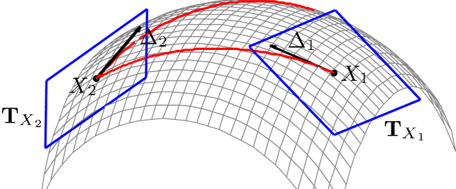
Fig. 1: Pictorial depiction of the main algorithmic procedure for the Grassmannian $\operatorname*{Gr}(3,1)$, which is simply the sphere $S^{2}$.

11 Numerical experiments and computational complexity

All algorithms described here and the object oriented Grassmann classes required for them are available for download as two matlab packages [50] and [51]. We encourage our readers to try them out.

11.1 Initialization and stopping condition

We will now test the actual performance of our algorithms with a few large numerical examples. All algorithms in a given test are started with the same initial points on a Grassmannian, represented as truncated singular matrices from the hosvd and a number of additional higher order orthogonal iterations—hooi iterations [15, 16], which are introduced to make the initial Hessian of $\Phi$ negative definite. The number of initial hooi iterations ranges between $5$ and $50$ depending on the size of the problem. The bfgs algorithm is either started with (possibly a modification of) the exact Hessian or a scaled identity matrix according to [46, pp. 143]. The l-bfgs algorithm is always started with a scaled identity matrix but one can modify the number of columns $m$ in the matrices representing the Hessian approximation, see equation (40). This number is between $5$ and $30$. Although we use the hosvd to initialize our algorithms, any other reasonable initialization procedure would work as long as the initial Hessian approximate is negative definite. The quasi-Newton methods can be used as stand-alone algorithms for solving the tensor approximation problem as well as other problems defined on Grassmannians.

In the following figures, the $y$-axis measures the norm of the relative gradient, i.e. $\lVert\nabla\Phi(X)\rVert/\lVert\Phi(X)\rVert$, and the $x$-axis shows iterations. This ratio is also used as our stopping condition, which typically requires that $\lVert\nabla\Phi(X)\rVert/\lVert\Phi(X)\rVert\approx 10^{-13}$, the machine precision of our computer. At a true local maximizer the gradient of the objective function is zero and its Hessian is negative definite. In the various figures we present convergence results for four principally different algorithms. These are (1) quasi-Newton-Grassmann with bfgs, (2) quasi-Newton-Grassmann with l-bfgs, (3) Newton-Grassmann, denoted with ng and (4) hooi which is an alternating least squares approach. In addition, the tags for bfgs methods may be accompanied by i or h indicating whether the initial Hessian was a scaled identity matrix or the exact Hessian, respectively.

11.2 Experimental results

We run all our numerical experiments in matlab on a MacBook with a $2.4$-GHz Intel Core 2 Duo processor and $4$ GB of physical memory.

Figure 2 shows convergence results for two tests with tensors generated with $N(0,1)$-distributed values.

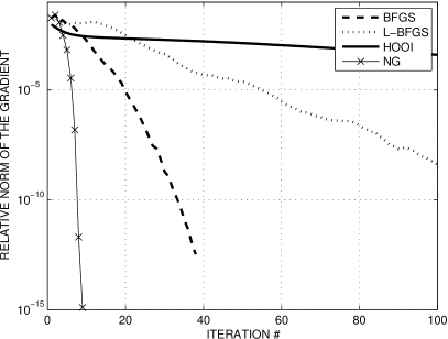
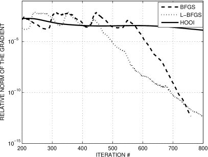
Fig. 2: Left: A $20\times 20\times 20$ tensor is approximated by a rank-$(5,5,5)$ tensor. bfgs initiated with the exact Hessian; In l-bfgs $m=5$. Right: A $100\times 100\times 100$ tensor is approximated by a rank-$(5,10,20)$ tensor. In this case the initial Hessian is a scaled identity and $m=10$.

In the left plot a $20\times 20\times 20$ tensor is approximated with a rank-$(5,5,5)$ tensor. One can observe superlinear convergence in the bfgs method. The right plot shows convergence results of a $100\times 100\times 100$ tensor approximated with a rank-$(5,10,20)$ tensor. Both bfgs and l-bfgs methods exhibit rapid convergence in the vicinity of a stationary point.

Figure 3 (left) shows convergence for an even larger $200\times 200\times 200$ tensor approximated by a tensor of rank-$(10,10,10)$ using l-bfgs with $m=20$.

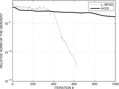
Fig. 3: Left: Convergence plots of a $200\times 200\times 200$ tensor approximated by a rank-$(10,10,10)$ tensor. Right: Effect of varying $m$ in l-bfgs. A $50\times 50\times 50$ tensor approximated by a rank-$(20,20,20)$ tensor with $m=5,10,15,20,25,30$.

In the right plot we approximate a $50\times 50\times 50$ tensor by a rank-$(20,20,20)$ tensor where we vary over a range of values of $m$ in the l-bfgs algorithm, namely, $m=5,10,15,20,25,30$. $m=5$ gives (in general) slightly poorer performance, otherwise the different runs cannot be distinguished. In other words, our Grassmann l-bfgs algorithm can in practice work as well as our Grassmann bfgs algorithm, just as one would expect (from the numerical experiments performed) in the Euclidean case.

Figure 4 shows convergence plots for two symmetric tensor approximation problems.

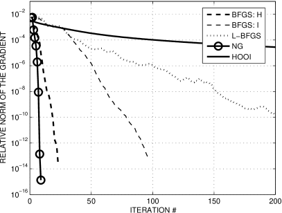
Fig. 4: Left: A $50\times 50\times 50$ symmetric tensor is approximated by a rank-$5$ symmetric tensor; $m=10$. Right: Here we have a $100\times 100\times 100$ symmetric tensor approximated by a rank-$20$ symmetric tensor; $m=10$.

In the left plot we approximate a symmetric $50\times 50\times 50$ tensor by a rank-$5$ symmetric tensor. We observe that bfgs initialized with the exact Hessian (bfgs:h tag) converges much more rapidly, almost as fast as the Newton-Grassmann method, than when initialized with a scaled identity matrix (bfgs:i tag). In the right plot we give convergence results for a $100\times 100\times 100$ symmetric tensor approximated by a rank-$20$ symmetric tensor. In both cases $m=10$.

In Figure 5 we show the performance of a local coordinate implementation of the bfgs algorithm on problems with $4$-tensors. The first plot shows convergence results for a $50\times 50\times 50\times 50$ tensor approximated by a rank-$(5,5,5,5)$ tensor. The second convergence plot is for a symmetric $4$-tensor with the same dimensions approximated by a symmetric rank-$5$ tensor.

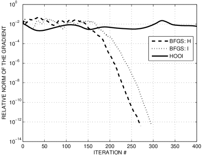
Fig. 5: Left: A $50\times 50\times 50\times 50$ tensor is approximated by a rank-$(5,5,5,5)$ tensor. Right: Here we have a $50\times 50\times 50\times 50$ symmetric tensor approximated by a rank-$5$ symmetric tensor.

Again the h and i tags indicate whether the exact Hessian or a scaled identity is used for initialization.

We end this section with two unusual examples to illustrate the extent of our algorithms’ applicability: a high order tensor and an objective function that includes tensors of different orders. The left plot in Figure 6 is a high-order example: it shows the convergence of bfgs verses hooi when approximating an order-$10$ tensor with dimensions $5\times 5\times\cdots\times 5$ with a rank-$(2,2,\dots,2)$ tensor. The right plot in Figure 6 has an unusual objective function that involves an order-$2$, an order-$3$, and an order-$4$ tensor,

$$\Phi(X)=\frac{1}{2!}\lVert S_{2}\cdot(X,X)\rVert_{F}^{2}+\frac{1}{3!}\lVert\mathcal{S}_{3}\cdot(X,X,X)\rVert_{F}^{2}+\frac{1}{4!}\lVert\mathcal{S}_{4}\cdot(X,X,X,X)\rVert_{F}^{2}$$

where $S_{2}$ is a $30\times 30$ symmetric matrix, $\mathcal{S}_{3}$ is a $30\times 30\times 30$ symmetric $3$-tensor, and $\mathcal{S}_{4}$ is a $30\times 30\times 30\times 30$ symmetric $4$-tensor. Such objective functions have appeared in independent component analysis with soft whitening [18] and in principal cumulants components analysis [44, 41] where $S_{2},\mathcal{S}_{3},\mathcal{S}_{4}$ measure the multivariate variance, kurtosis, skewness respectively (cf. Example 2).

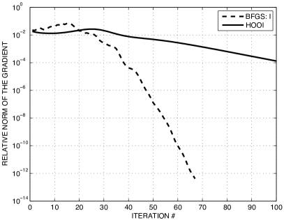
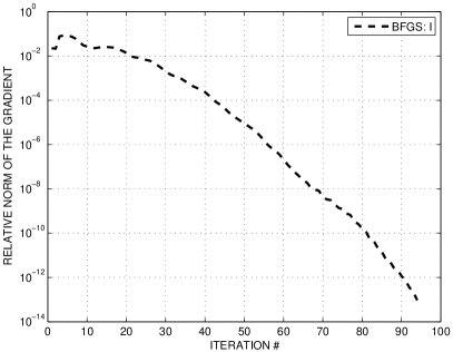
Fig. 6: Left: A $5\times 5\times\cdots\times 5$ tensor of order-10 is approximated with a rank-$(2,2,\dots,2)$. Right: A ‘simultaneous’ rank-$5$ approximation of a weighted sum of tensors of orders $2$, $3$, and $4$.

In both examples we observe a fast rate of convergence at the vicinity of a local minimizer for the bfgs algorithm.

It is evident from the convergence plots here that bfgs and l-bfgs have faster rate of convergence compared with hooi. The Newton-Grassmann algorithm takes few iterations but is computationally more expensive, specifically for larger problems. Our implementation of the different algorithms in matlab give shortest runtime for the bfgs and l-bfgs methods. The time for one iteration of bfgs, l-bfgs and hooi is of the same magnitude for smaller problems. In larger problems, the l-bfgs performs much faster than all other methods.

Our algorithms use the basic arithmetic and data types in the TensorToolbox [4] for convenience. We use our own object-oriented routines for operations on Grassmannians and product of Grassmannians, e.g. geodesic movements and parallel transports [51]. We note that there are several different ways to implement bfgs updates [46]; for simplicity reasons, we have chosen to update the inverse of the Hessian approximation. A possibly better alternative will be to update the Cholesky factors of the approximate Hessians so that one may monitor the approximate Hessians for indefiniteness during the iterations [23, 28, 7].

11.3 Computational complexity, curse of dimensionality, and convergence

The Grassmann quasi-Newton methods presented in this report all fit within the procedural framework given in Algorithm 1.

Algorithm 1 Algorithmic framework for bfgs and l-bfgs on Grassmannians.

  Given tensor $\mathcal{A}$ and starting points $(X_{0},Y_{0},Z_{0})\in\operatorname*{Gr}^{3}$ and an initial Hessian $H_{0}$

  repeat

     1 Compute the Grassmann gradient.

     2 Parallel transport the Hessian approximation to the new point.

     3 Update the Hessian or its compact representation.

     4 Solve the quasi-Newton equations to obtain $\Delta=(\Delta_{x},\Delta_{y},\Delta_{z})$.

     5 Move the points $(X_{k},Y_{k},Z_{k})$ along the geodesic curve given by $\Delta$.

  until  $\lVert\nabla\widehat{\Phi}\rVert/\Phi<$ TOL

General case

In analyzing computational complexity, we will assume for simplicity that $\mathcal{A}$ is a general $n\times n\times n$ $3$-tensor being approximated with a rank-$(r,r,r)$ $3$-tensor. A problem of these dimensions will give rise to a $3nr\times 3nr$ Hessian matrix in global coordinates and a $3(n-r)r\times 3(n-r)r$ Hessian matrix in local coordinates. Table 1 gives approximately the amount of computations required in each step of Algorithm 1. Recall that in l-bfgs $m$ is a small number, see Section 7.

	bfgs-gc	bfgs-lc	l-bfgs
1	$6n^{3}r+12n^{2}r^{2}$	$6n^{3}r+{6}n^{2}r^{2}+6n(n-r)r^{3}$	$6n^{3}r+12n^{2}r^{2}$
2	$18n^{3}r^{2}$	—	$12n^{2}rm$
3	$36n^{2}r^{2}$	$36(n-r)^{2}r^{2}$	—
4	$18n^{2}r^{2}$	$18(n-r)^{2}r^{2}$	$24nrm$

Table 1: Computational complexity of the bfgs-gc (global coordinates), bfgs-lc (local coordinates) and l-bfgs algorithms. The numbers in the first column correspond to the steps in Algorithm 1.

We have omitted terms of lower asymptotic complexity as well as the cost of point 5 since that is negligible compared with the costs of points 1–4. For example, the geodesic movement of $X_{k}$ requires the thin svd $U_{x}\Sigma_{x}V_{x}^{\mathsf{T}}=\Delta_{x}\in\mathbb{R}^{n\times r}$ which takes $6nr^{2}+20r^{3}$ flops (floating point operations) [29]. On the other hand, given the step length $t$ and $U,\Sigma,V$ in (18), the actual computation of $X(t)$ amounts to only $4nr^{2}$ flops.

Symmetric case

The symmetric tensor approximation problem involves the determination of one $n\times r$ matrix, resulting in an $nr\times nr$ Hessian in global coordinates and an $(n-r)r\times(n-r)r$ Hessian in local coordinates. Therefore the complexity of the symmetric problem differs only by a constant factor from that of the general case.

Curse of dimensionality

The approximation problem will suffer from the curse of dimensionality when the order of a tensor increases. In general, an $n\times\dots\times n$ order-$k$ tensor requires the storage of $n^{k}$ entries in memory. The additional memory requirement, mainly for storing the Hessian, is of order $O(n^{2}r^{2}k^{2})$ for the bfgs methods and $O(2nrkm)$ for the l-bfgs method, respectively. In the current approach we assume that the tensor is explicitly given. Our proposed algorithms are applicable as long as the given tensor fits in memory. There have been various proposals to deal with the curse of dimensionality using tensors [35, 36, 48]. For cases where the tensor is represented in compact or functional forms our methods can take direct advantage of these simply by computing the necessary gradients (and Hessians) using the specific representations. In fact this was considered in [43] for symmetric tensor approximations.

Convergence

There is empirical evidence suggesting that als based algorithms have fast convergence rate for specific tensors. This was also pointed out in [12]. These are tensors that have inherently low multilinear rank and the approximating tensor has the correct low ranks, or tensors that have fast decay in its multilinear singular values [15], or a substantial gap in the multilinear singular values at the site of truncation, e.g. the source tensor is given by a low rank tensor with noise added. On the other hand not all tensors have gaps or fast decaying multilinear singular vales. This is specifically true for sparse tensors. It is still desirable to obtain low rank approximations for these “more difficult” tensors. And on these tensors als performs very poorly, but methods using first and second order derivatives of the objective function, including the methods presented in this paper perform good. Among the methods that are currently available, quasi-Newton methods presented in this paper have the best computational efficiency.

12 Related work

There are several different approaches to solve the tensor approximation problem. In this section we will briefly describe them and point out the main differences with our work. The algorithms most closely related to the quasi-Newton methods are given in [25, 34, 33]. All three references address the best low rank tensor approximation based on the Grassmannian structure of the problem and use explicit computation of the Hessian. The obtained Newton equations are solved either fully [25, 34] or approximately [33]. In the latter case the authors used a truncated conjugate gradient approach to approximately solve the Newton equations. The iterates are updated using the more general notion of retractions instead of taking a step along the geodesic on the manifold. In addition a trust region scheme is incorporated making the procedure more stable with respect to occasional indefinite Hessians. The computation of the Hessian is a limiting factor in these algorithms. This is the case even when the Hessian is not formed explicitly but used implicitly via its action on a tangent. In our experiments, on moderate-sized problems, e.g. $3$-tensors of dimensions around $20\times 20\times 20$, the bfgs methods noticeably outperformed Hessian-based methods; and for dimensions around $100\times 100\times 100$, we were unable to get any methods relying on Hessians to work despite our best efforts.

There is a different line of algorithms for related tensor approximation problems based on als and mutltigrid accelerated als [35, 36]. In our experience, the convergence of als-type methods depend on the decay of the multilinear singular values of the given tensor. The exact dependence is unclear but the relation seems to be that the faster the decay, the faster the convergence of als. In this regard the class of functions and operators considered in [35, 36] appears to possess these favorable properties.

Yet a third approach to obtain low multilinear rank tensor approximations are the cross methods in [49, 48, 26]. The novelty of such methods is that they discard some given information and retain only a fraction of the original tensor, and as such it is markedly different from our approach, which uses all given information to achieve maximal accuracy. In addition, there is an assumption on the tensor that there exist approximations within pre-specified bounds and of specific low ranks while we make no such assumptions.

13 Conclusion

In this paper we studied quasi-Newton algorithms adapted to optimization problems on Riemannian manifolds. More specifically, we proposed algorithms with bfgs and l-bfgs updates on a product of Grassmannians that (1) respect the Riemannian metric structure and (2) require only standard matrix operations in their implementations. Two different algorithmic implementations are presented: one based on local/intrinsic coordinates while the other one uses global/embedded coordinates. In particular, our use of local coordinates is a novelty not previously explored in other manifold optimization [1, 2, 24, 27]. We proved the optimality of our Grassmannian bfgs updates in local coordinates, showing that the well-known bfgs optimality [21, 22] extends to Grassmannian and products of Grassmannians.

We also applied these algorithms to the problem of determining a best multilinear rank approximation of a tensor and the analogous (but very different) problem for a symmetric tensor. While a Newton version of this was proposed in [25], here we make substantial improvements with respect to the Grassmann-Newton algorithm in terms of speed and robustness. Furthermore, we presented specialized algorithms that take into account the symmetry in the multilinear approximation of symmetric tensors and related problems. In addition to the numerical experiments in this paper, we have made our codes freely available for download [50, 51] so that the reader may verify the speed, accuracy, and robustness of these algorithms for himself.

Appendix A Notation for tensor contractions

In this section we define the contracted tensor product notation used throughout this paper. For given third order tensors $\mathcal{A}$ and $\mathcal{B}$ we define the following contracted products:

$$\mathcal{C}=\langle\mathcal{A},\mathcal{B}\rangle_{1},\qquad c_{ijkl}=\sum_{\lambda}a_{\lambda ij}b_{\lambda kl}.$$ (59)

When contracting several indices, with the corresponding indices of the two arguments being the same, we write

$$\mathcal{C}=\langle\mathcal{A},\mathcal{B}\rangle_{1,2},\qquad c_{ij}=\sum_{\lambda,\nu}a_{\lambda\nu i}b_{\lambda\nu j}.$$ (60)

The subscript ‘1’ in $\langle\mathcal{A},\mathcal{B}\rangle_{1}$ and subscripts ‘1,2’ in $\langle\mathcal{A},\mathcal{B}\rangle_{1,2}$ indicate that the contraction is over the first index and both the first and second indices respectively. If instead the contraction is to be performed on different indices, we write

$$\mathcal{C}=\langle\mathcal{A},\mathcal{B}\rangle_{1;2},\quad c_{ijkl}=\sum_{\lambda}a_{\lambda ij}b_{k\lambda l}\quad\text{or}\quad\mathcal{C}=\langle\mathcal{A},\mathcal{B}\rangle_{1,3;2,1},\quad c_{ij}=\sum_{\lambda,\nu}a_{\lambda i\nu}b_{\nu\lambda j}.$$

The subscripts indicating the indices to be contracted are separated by a semicolon. It is also convenient to introduce a notation when contraction is performed in all but one or a few indices. For example the products in (60) and (60) may also be written

$$\langle\mathcal{A},\mathcal{B}\rangle_{1,2}=\langle\mathcal{A},\mathcal{B}\rangle_{-3}\quad\text{or}\quad\langle\mathcal{A},\mathcal{B}\rangle_{1}=\langle\mathcal{A},\mathcal{B}\rangle_{-(2,3)}.$$

References

- [1] P.-A. Absil, C. G. Baker, and K. A. Gallivan, Trust-region methods on Riemannian manifolds, Found. Comput. Math., 7 (2007), no. 3, pp. 303–330.
- [2] P.-A. Absil, R. Mahony, and R. Sepulchre, Optimization Algorithms on Matrix Manifolds, Princeton University Press, Princeton, NJ, 2008.
- [3] E. Anderson, Z. Bai, C. H. Bischof, J. W. Demmel, J. J. Dongarra, J. J. Du Croz, A. Greenbaum, S. J. Hammarling, A. McKenney, S. Ostrouchov, and D. C. Sorensen, LAPACK Users’ Guide, 3rd Ed., SIAM, Philadelphia, PA, 1999.
- [4] B. W. Bader and T. G. Kolda, Algorithm 862: MATLAB tensor classes for fast algorithm prototyping, ACM Trans. Math. Software, 32 (2006), no. 4, pp. 635–653.
- [5] W. M. Boothby, An Introduction to Differentiable Manifolds and Riemannian Geometry, 2nd Ed., Academic Press, Orlando, FL, 1986.
- [6] R. H. Byrd, J. Nocedal, and R. B. Schnabel, Representations of quasi-Newton matrices and their use in limited memory methods, Math. Program., 63 (1994), no. 2, pp. 129–156.
- [7] S. H. Cheng and N. J. Higham, A modified cholesky algorithm based on a symmetric indefinite factorization, SIAM J. Matrix Anal. Appl., 19 (1998), no. 4, pp. 1097–1110.
- [8] P. Comon, G. Golub, L.-H. Lim, and B. Mourrain, Symmetric tensors and symmetric tensor rank, SIAM J. Matrix Anal. Appl., 39 (2008), no. 3, pp. 1254–1279.
- [9] ———, Genericity and rank deficiency of high order symmetric tensors, Proc. IEEE Int. Conf. Acoustics, Speech, and Signal Process. (ICASSP ’06), 31 (2006), pp. 125–128.
- [10] P. Comon and B. Mourrain, Decomposition of quantics in sums of powers of linear forms, Signal Process., 53 (1996), pp. 93–107.
- [11] L. Conlon, Differentiable Manifolds, 2nd Ed., Birkhäuser, Boston, MA, 2001.
- [12] L. De Lathauwer, Tucker compression, parallel factor analysis and block term decompositions: New results, European Meeting on Challenges in Modern Massive Data Sets (EMMDS ’09), Copenhagen, Denmark, 2009.
- [13] ———, Signal Processing Based on Multilinear Algebra, Ph.D. thesis, Department of Electrical Engineering, Katholieke Universiteit Leuven, Leuven, Belgium, 1997.
- [14] L. De Lathauwer, B. De Moor, and J. Vandewalle, An introduction to independent component analysis, J. Chemometrics, 14 (2000), pp. 123–149.
- [15] ———, A multilinear singular value decomposition, SIAM J. Matrix Anal. Appl., 21 (2000), no. 4, pp. 1253–1278.
- [16] ———, On the best rank- and rank- approximation of higher-order tensors, SIAM J. Matrix Anal. Appl., 21 (2000), no. 4, pp. 1324–1342.
- [17] L. De Lathauwer, L. Hoegaerts, and J. Vandewalle, A Grassmann-Rayleigh quotient iteration for dimensionality reduction in ICA, Proc. Int. Conf. Independent Component Analysis and Blind Signal Separation (ICA ’04), 5 (2004), pp. 335–342.
- [18] L. De Lathauwer and J. Vandewalle, Dimensionality reduction in higher-order signal processing and rank- reduction in multilinear algebra, Linear Algebra Appl., 391 (2004), pp. 31–55.
- [19] ———, Dimensionality reduction in ICA and rank- reduction in multilinear algebra, Proc. Int. Conf. Independent Component Analysis and Blind Signal Separation (ICA ’04), 5 (2004), pp. 295–302.
- [20] V. De Silva and L.-H. Lim, Tensor rank and the ill-posedness of the best low-rank approximation problem, SIAM J. Matrix Anal. Appl., 30 (2008), no. 3, pp. 1084–1127.
- [21] J. E. Dennis and J. Moré, Quasi-newton methods, motivation and theory, SIAM Rev., 19 (1997), no. 1, pp. 46–89.
- [22] J. E. Dennis and R. B. Schnabel, A new derivation of symmetric positive definite secant updates, Nonlinear Program., 4 (1981), pp. 167–199.
- [23] ———, Numerical Methods for Unconstrained Optimization and Nonlinear Equations, SIAM, Philadelphia, PA, 1996.
- [24] A. Edelman, T. A. Arias, and S. T. Steven, The geometry of algorithms with orthogonality constraints, SIAM J. Matrix Anal. Appl., 20 (1999), no. 2, pp. 303–353.
- [25] L. Eldén and B. Savas, A Newton–Grassmann method for computing the best multilinear rank- approximation of a tensor, SIAM J. Matrix Anal. Appl., 31 (2009), no. 2, pp. 248–271.
- [26] H.-J. Flad, B. N. Khoromskij, D. Savostianov, and E. Tyrtyshnikov, Verification of the cross 3D algorithm on quantum chemistry data, Russian J. Numer. Anal. Math. Modelling, 4 (2008), pp. 1–16.
- [27] D. Gabay, Minimizing a differentiable function over a differential manifold, J. Optim. Theory Appl., 37 (1982), no. 2, pp. 177–219.
- [28] D. Goldfarb, Factorized variable metric methods for unconstrained optimization, Math. Comp., 30 (1976), no. 136, pp. 796–811.
- [29] G. H. Golub and C. F. Van Loan, Matrix Computations, 3rd Ed., Johns Hopkins University Press, Baltimore, MD, 1996.
- [30] W. Greub, Multilinear Algebra, 2nd Ed., Springer-Verlag, New York, NY, 1978.
- [31] F. L. Hitchcock, The expression of a tensor or a polyadic as a sum of products, J. Math. Phys., 6 (1927), no. 1, pp. 164–189.
- [32] M. Ishteva, L. De Lathauwer, P.-A. Absil, and S. Van Huffel, Dimensionality reduction for higher-order tensors: Algorithms and applications, Int. J. Pure Appl. Math., 42 (2008), no. 3, pp. 337–343.
- [33] ———, Best low multilinear rank approximation of higher-order tensors, based on the Riemannian trust-region scheme, Tech. Rep., 09-142, ESAT-SISTA, Katholieke Universiteit Leuven, Leuven, Belgium, 2009.
- [34] ———, Differential-geometric newton algorithm for the best rank- approximation of tensors, Numer. Algorithms, 51 (2009), no. 2, pp. 179–194.
- [35] B. N. Khoromskij and V. Khoromskaia, Low rank Tucker-type tensor approximation to classical potentials, Cent. Eur. J. Math., 5 (2007), no. 3, pp. 523–550.
- [36] ———, Multigrid accelerated tensor approximation of function related multidimensional arrays, SIAM J. Sci. Comput., 31 (2009), no. 4, pp. 3002–3026.
- [37] E. Kofidis and P. A. Regalia, On the best rank-1 approximation of higher-order supersymmetric tensors, SIAM J. Matrix Anal. Appl., 23 (2002), no. 3, pp. 863–884.
- [38] T. G. Kolda and B. W. Bader, Tensor decompositions and applications, SIAM Rev., 51(2009), no. 3, pp. 455–500.
- [39] S. Lang, Algebra, Rev. 3rd Ed., Springer-Verlag, New York, NY, 2002.
- [40] R. Lehoucq, D. Sorensen, and C. Yang, ARPACK Users’ Guide, SIAM, Philadelphia, PA, 1998.
- [41] L.-H. Lim and J. Morton, Cumulant component analysis: a simultaneous generalization of PCA and ICA, Computational Algebraic Statistics, Theories and Applications (CASTA ’08), Kyoto University, Kyoto, Japan, December 10–11 2008.
- [42] E. Lundström and L. Eldén, Adaptive eigenvalue computations using Newton’s method on the Grassmann manifold, SIAM J. Matrix Anal. Appl., 23 (2002), no. 3, pp. 819–839.
- [43] J. Morton, Scalable implicit symmetric tensor approximation, preprint, 2010.
- [44] J. Morton and L.-H. Lim, Principal cumulant components analysis, preprint, 2009.
- [45] M. Mørup, L. K. Hansen, S. M. Arnfred, ERPWAVELAB: A toolbox for multi-channel analysis of time-frequency transformed event related potentials, J. Neurosci. Methods, 161 (2007), no. 2, pp. 361–368.
- [46] J. Nocedal and S. J. Wright, Numerical Optimization, 2nd Ed., Springer, New York, NY, 2006.
- [47] L. Omberg, G. H. Golub, and O. Alter, A tensor higher-order singular value decomposition for integrative analysis of DNA microarray data from different studies, Proc. Natl. Acad. Sci., 104 (2007), no. 47, pp. 18371–18376.
- [48] I. V. Oseledets, Compact matrix form of the -dimensional tensor decomposition, Tech. Rep., Institute of Numerical Mathematics, Russian Academy of Science, Moscow, Russia, 2009.
- [49] I. V. Oseledets, D. V. Savostianov, and E. E. Tyrtyshnikov, Tucker dimensionality reduction of three-dimensional arrays in linear time, SIAM J. Matrix Anal. Appl., 30 (2008), no. 3, pp. 939–956.
- [50] B. Savas, Algorithm package manual: Best low rank tensor approximation, Department of Mathematics, Linköping Univeristy, Linköping, Sweden, 2008. (http://www.mai.liu.se/~besav/soft.html)
- [51] ———, Toolbox for Grassmann manifold computations, Department of Mathematics, Linköping Univeristy, Linköping, Sweden, 2008. (http://www.mai.liu.se/~besav/soft.html)
- [52] L. Simonsson, Subspace Computations via Matrix Decompositions and Geometric Optimization, Linköping studies in science and technology, 1052, Linköping University, Linköping, Sweden, 2007.
- [53] A. Smilde, R. Bro, and P. Geladi, Multi-way Analysis: Applications in the Chemical Sciences, John Wiley, West Sussex, England, 2004.
- [54] L. R. Tucker, Some mathematical notes on three-mode factor analysis, Psychometrika, 31 (1966), no. 3, pp. 279–311.
- [55] M. A. O. Vasilescu and D. Terzopoulos, Multilinear subspace analysis of image ensembles, Proc. Comput. Vis. Pattern Recognition Conf. (CVPR ’03), 2 (2003), pp. 93–99.
- [56] T. Yokonuma, Tensor Spaces and Exterior Algebra, AMS, Providence, RI, 1992.