Tracking azimuthons in nonlocal nonlinear media

Abstract

We study the formation of azimuthons, i.e., rotating spatial solitons, in media with nonlocal focusing nonlinearity. We show that whole families of these solutions can be found by considering internal modes of classical non-rotating stationary solutions, namely vortex solitons. This offers an exhaustive method to identify azimuthons in a given nonlocal medium. We demonstrate formation of azimuthons of different vorticities and explain their properties by considering the strongly nonlocal limit of accessible solitons.

1 Introduction

There has been growing interest in studies of propagation of optical beams in nonlocal media. These are media where the nonlinear response of the material in a specific spatial location is determined not only by the wave intensity in the same location but also in its neighborhood. The extent of this neighborhood in comparison to the beam width determines the degree of nonlocality. The nonlinear nonlocal response appears to be ubiquitous to many physical settings. For instance, it is common to media where certain transport processes such as heat (Dabby and Whinnery, 1968; Litvak et al, 1975; Davydova and Fishchuk, 1995) or charge transfer (Calvo et al, 2002), diffusion and/or drift of atoms (Suter and Blasberg, 1993; Skupin et al, 2007) are responsible for the nonlinearity. It also occurs in systems involving long-range interaction of atoms or molecules as it is the case of nematic liquid crystals (Conti et al, 2004, 2003) or dipolar Bose-Einstein condensate (Goral et al, 2000; Nath et al, 2007; Koch et al, 2008). It has been shown that nonlocal nonlinear response has profound consequences on the wave propagation and formation of localized structures (Krolikowski et al, 2004). In particular, nonlocality prevents collapse by providing a stabilization mechanism and enables robust existence of various types of localized structures and spatial solitons (Kolchugina et al, 1980; Bang et al, 2002; Briedis et al, 2005; Skupin et al, 2006; Lashkin, 2007; Lashkin et al, 2007). In local nonlinear media the wave perturbation in a particular place affects the nonlinearity which in turn, influences the wave itself often instigating its breakup or spatial transformation (Desyatnikov et al, 2005b). On the other hand, in nonlocal media such perturbation is spatially averaged, and hence has a much weaker impact on the wave itself, leading to its stabilization. In particular, it has been shown that nonlocality support stable propagation of optical vortices, and multi-peak solitonic structures which are structurally unstable in material with local response (Buccoliero et al, 2008, 2007b, 2007a). A range of particular types of fundamental as well as higher order nonlocal solitons and their interactions have been even demonstrated experimentally in materials with nonlocal response of thermal origin (Rotschild et al, 2006b, a). Recently, it has been also shown theoretically that spatial nonlocal response enables realization of the so called azimuthons i.e. multiple peak ring-shaped solitons which exhibit angular rotation in propagation (Desyatnikov et al, 2005a; Lopez-Aguayo et al, 2006b, a; Skupin et al, 2008). While few specific types of azimuthons have been investigated in various nonlocal models, using variational techniques mentioned above as well as numerical relaxation procedure (Lashkin, 2008b, a), no general approach to find stable nonlocal azimuthons has been demonstrated so far. In this work we study the formation of azimuthons in nonlocal media with gaussian response. We show that whole families of these solitons can be tracked down by analyzing bifurcations originating from the nonlinear optical potential of vortex solitons.

2 Azimuthons

We consider physical systems governed by the two-dimensional nonlocal nonlinear Schrödinger equation

$$i\frac{\partial}{\partial z}\psi+\Delta_{\perp}\psi+\theta\psi=0.$$ (1)

where $\theta$ represents the spatially nonlocal nonlinear response of the medium. Its form depends on the details of a particular physical system. In the following, we will assume that the nonlinear response $\theta$ can be expressed in terms of the nonlocal response function $R(r)$

$$\theta=\iint R(|\vec{r}-\vec{r}^{\prime}|)\left|\psi(\vec{r}^{\prime},z)\right|^{2}d^{2}\vec{r}^{\prime},$$ (2)

where $\vec{r}=x\vec{e}_{x}+y\vec{e}_{y}$ denotes the transverse coordinates. In this work we will use the so-called Gaussian model of nonlocality as an illustrative example,

$$\theta=\frac{1}{2\pi}\iint\mathrm{e}^{-\frac{|\vec{r}-\vec{r}^{\prime}|^{2}}{2}}\left|\psi(\vec{r}^{\prime},z)\right|^{2}d^{2}\vec{r}^{\prime}.$$ (3)

However, the proposed solutions should exist in many other nonlocal models (Litvak et al, 1975; Rotschild et al, 2006a; Suter and Blasberg, 1993; Skupin et al, 2007; Assanto and Peccianti, 2003; Conti et al, 2004; Peccianti et al, 2006; Denschlag et al, 2000; Pedri and Santos, 2005; Koch et al, 2008).

Azimuthons are a straightforward generalization of the usual ansatz for stationary solutions (solitons) (Desyatnikov et al, 2005a). They represent spatially rotating structures and hence involve an additional parameter, the angular frequency $\Omega$ (see also Skryabin et al (2002))

$$\psi(r,\phi,z)=U(r,\phi-\Omega z)\mathrm{e}^{i\lambda z},$$ (4)

where $U$ is the complex amplitude function and $\lambda$ the propagation constant. For $\Omega=0$, azimuthons become ordinary (nonrotating) solitons. The simplest example of a family of azimuthons is the one connecting the dipole soliton with the single charged vortex soliton (Lopez-Aguayo et al, 2006b). A single charged vortex consists of two equal-amplitude dipole-shaped structures with the relative phase of $\pi/2$ representing real and imaginary part of $U$. If these two components differ in amplitudes the resulting structure forms a ”rotating dipole” azimuthon. If one of the components is zero we deal with the nonrotating dipole soliton. In the following we will denote the amplitude ratio of these two vortex components by $\alpha$, which also determines the angular modulation depth of the resulting ring-like structure by “$1-\alpha$”. When higher order (e.g. single charged triple-hump) azimuthons are concerned, we can not always identify the angular modulation depth with amplitude ratios of real and imaginary part of $U$. Hence we define the generalized structural parameter $\alpha$ as

$$\alpha=1-\frac{\min_{\phi}|U(r_{\rm max},\phi)|}{|U(r_{\rm max},\phi_{\rm max})|},$$ (5)

where the tuple $(r_{\rm max},\phi_{\rm max})$ denotes the coordinates of the maximum value $\max_{r,\phi}{|U|}$.

After inserting the ansatz (4) into Eqs. (1) and (2), multiplying with $U^{*}$ and $\partial_{\phi}U^{*}$ resp., and integrating over the transverse coordinates we end up with

$$-\lambda M+\Omega L_{z}+I+N =0$$ (6a)

$$-\lambda L_{z}+\Omega M^{\prime}+I^{\prime}+N^{\prime} =0.$$ (6b)

This system relates the propagation constant $$\lambda \Omega$$ and the rotation frequency of the azimuthons to integrals over their stationary amplitude profiles, namely

$$M =\iint\left|U(\vec{r})\right|^{2}d^{2}\vec{r}$$ (6c)

$$L_{z} =-i\iint U^{*}(\vec{r})\frac{\partial}{\partial\phi}U(\vec{r})d^{2}\vec{r}$$ (6d)

$$I =\iint U^{*}(\vec{r})\Delta_{\perp}U(\vec{r})d^{2}\vec{r}$$ (6e)

$$N =\iiiint R(|\vec{r}-\vec{r}^{\prime}|)\left|U(\vec{r}^{\prime})\right|^{2}\left|U(\vec{r})\right|^{2}d^{2}\vec{r}^{\prime}d^{2}\vec{r}$$ (6f)

$$M^{\prime} =\iint\left|\frac{\partial}{\partial\phi}U(\vec{r})\right|^{2}d^{2}\vec{r}$$ (6g)

$$I^{\prime} =i\iint\left[\frac{\partial}{\partial\phi}U^{*}(\vec{r})\right]\Delta_{\perp}U(\vec{r})d^{2}\vec{r}$$ (6h)

$$N^{\prime} =i\iiiint R(|\vec{r}-\vec{r}^{\prime}|)\left|U(\vec{r}^{\prime})\right|^{2}\left[\frac{\partial}{\partial\phi}U^{*}(\vec{r})\right]U(\vec{r})d^{2}\vec{r}^{\prime}d^{2}\vec{r}.$$ (6i)

The first two quantities have straightforward physical meanings, namely ”mass” ($M$) and ”angular momentum” ($L_{z}$). We can formally solve for the rotation frequency and obtain (for an alternative derivation see (Rozanov, 2004)

$$\Omega=\frac{M\left(I^{\prime}+N^{\prime}\right)-L_{z}\left(I+N\right)}{L_{z}^{2}-MM^{\prime}}.$$ (7)

Note that this expression is undetermined for a vortex beam. For $\alpha=1$ [vortex soliton $V(r)\exp(iq\phi+i\lambda_{0}z$)], we can assume any value for $\Omega$ by just shifting the propagation constant $\lambda=\lambda_{0}+\Omega$ accordingly ($\lambda_{0}$ accounts for the propagation constant in the non-rotating laboratory frame). However, with respect to a particular azimuthon in the limit $\alpha\rightarrow 1$, the value of $\Omega$ is fixed. In what follows, we denote this value by $\Omega|_{\alpha=1}$.

3 Internal modes and azimuthons

In this section we will discuss the formation of azimuthons via the process of bifurcation from a stationary non-rotating soliton solution, namely a vortex. We assume a certain deformation of the soliton profile while going over from the vortex to azimuthons in the limit $\alpha\rightarrow 1$. Therefore it has to be the shape of vortex deformation which determines $\Omega$, since a vortex formally allows for all possible rotation frequencies (see the discussion on shifting $\lambda$ at the end of Sec. 2).

Let us now look at the azimuthon originating (bifurcating) from a vortex soliton with charge $q$. For this purpose, we recall the eigenvalue problem for internal modes of the nonlinear potential $\theta$ which is usually treated in the context of linear stability of nonlinear soliton solutions (Firth and Skryabin, 1997; Desyatnikov et al, 2005b). We introduce a small perturbation $\delta V$ to the vortex soliton $V$,

$$\psi=\left(V+\delta V\right)\mathrm{e}^{iq\phi+i\lambda_{0}z},$$ (8)

plug it into Eqs. (1) and (2) and linearize those equations with respect to the perturbation. Note that the perturbation $\delta V(r,\phi,z)$ is complex, whereas the vortex profile $V(r)$ is real (w.l.o.g.). The resulting evolution equation for the perturbation $\delta V$ is then given by

$$\begin{split}\left[i\frac{\partial}{\partial z}-\lambda_{0}+\frac{1}{r}\frac{\partial}{\partial r}\left(r\frac{\partial}{\partial r}\right)+\frac{1}{r^{2}}\left(\frac{\partial}{\partial\phi}+iq\right)^{2}+\iint R(|\vec{r}-\vec{r}^{\prime}|)V^{2}(r^{\prime})d^{2}\vec{r}^{\prime}\right]\delta V&\\ +V\iint R(|\vec{r}-\vec{r}^{\prime}|)V(r^{\prime})\left[\delta V(\vec{r}^{\prime},z)+\delta V^{*}(\vec{r}^{\prime},z)\right]d^{2}\vec{r}^{\prime}&=0.\end{split}$$ (9)

With the ansatz

$$\delta V=\delta V_{1}(r)\mathrm{e}^{im\phi+i\kappa z}+\delta V^{*}_{2}(r)\mathrm{e}^{-im\phi-i\kappa^{*}z}$$ (10)

we derive the eigenvalue problem for the internal modes

$$\left[\frac{1}{r}\frac{\partial}{\partial r}\left(r\frac{\partial}{\partial r}\right)-\frac{(m+q)^{2}}{r^{2}}-\lambda_{0}+\iint R(|\vec{r}-\vec{r}^{\prime}|)V^{2}(r^{\prime})d^{2}\vec{r}^{\prime}\right]\delta V_{1}$$

$$+V\iint R(|\vec{r}-\vec{r}^{\prime}|)V(r^{\prime})\left[\delta V_{1}(r^{\prime})+\delta V_{2}(r^{\prime})\right]\cos[m(\phi-\phi^{\prime})]d^{2}\vec{r}^{\prime} =\kappa\delta V_{1}$$ (11a)

$$-\left[\frac{1}{r}\frac{\partial}{\partial r}\left(r\frac{\partial}{\partial r}\right)-\frac{(m-q)^{2}}{r^{2}}-\lambda_{0}+\iint R(|\vec{r}-\vec{r}^{\prime}|)V^{2}(r^{\prime})d^{2}\vec{r}^{\prime}\right]\delta V_{2}$$

$$-V\iint R(|\vec{r}-\vec{r}^{\prime}|)V(r^{\prime})\left[\delta V_{2}(r^{\prime})+\delta V_{1}(r^{\prime})\right]\cos[m(\phi-\phi^{\prime})]d^{2}\vec{r}^{\prime} =\kappa\delta V_{2}.$$ (11b)

Note that since $|\vec{r}-\vec{r}^{\prime}|=\sqrt{r^{2}+r^{\prime 2}-2rr^{\prime}\cos(\phi-\phi^{\prime})}$, all integrals in (11) are independent of $\phi$. Real-valued eigenvalues of Eq. (11) ($\kappa=\kappa^{*}$) are termed orbitally stable and the corresponding eigenvector $(\delta V_{1},\delta V_{2})$ can be chosen as real. If we perturb the vortex $V$ with an orbitally stable eigenvector, the resulting wave-function $\psi$ can be written in the form of Eq. (4) with $\Omega=-\kappa/m$ and $\lambda=\lambda_{0}-q\kappa/m$. Thus, it is possible to construct azimuthons in the vicinity of the vortex ($\alpha\approx 1$) from $\delta V$:

$$U(r,\phi)|_{z=0}=\left[V(r)+A_{r}\delta V_{1}(r)\mathrm{e}^{im\phi}+A_{r}\delta V_{2}(r)\mathrm{e}^{-im\phi}\right]\mathrm{e}^{iq\phi}.$$ (12)

Used as an initial condition in the propagation equation (1) this object is expected to rotate with an angular frequency $\Omega|_{\alpha=1}=-\kappa/m$. Here, $A_{r}>0$ was introduced as the amplitude of the perturbation $\delta V$ with respect to $V$. Since we are operating in a linearized system, the amplitude of the perturbation as a solution of Eq. (11) is not fixed (just the ratio between the components $\delta V_{1}$ and $\delta V_{2}$ is prescribed), but will eventually determine the value of the structural parameter $\alpha$. Generally speaking, the smaller the resulting $\alpha$ the greater the error in the constructed initial condition. However, the great robustness of the azimuthons, at least in the Gaussian model, allows one to use the initial condition (12) for quite large perturbation amplitudes $A_{r}$. Those strongly perturbed initial conditions result in oscillations of the azimuthon upon propagation. However, the azimuthon is structurally stable and does not decay into other soliton solutions like the single-hump ground state. Moreover, such initial conditions play a role of excellent ”initial guesses” for solver routines to find numerically exact azimuthons.

4 Higher order azimuthons

In a recent publication we have used the approach presented above to characterize the rotating dipole azimuthon, which connects the single charged vortex ($q=1$) to the stationary dipole soliton (Skupin et al, 2008). As already mentioned there, solving the eigenvalue problem (11) can be used as an exhaustive method for finding families of azimuthons which originate from a vortex soliton. However, it should be stressed that not all orbitally stable eigenvalues can be linked to a family of azimuthons. This is obvious for eigenvalues with $|\kappa|>|\lambda_{0}|$ in the continuous part of the spectrum. Hence, we can conclude that $|\Omega|_{\alpha=1}|<|\lambda_{0}|/m$ for azimuthons in the vicinity of the vortex ($\alpha\simeq 1$). Note that the parameter $m$ determines the number of humps of the rotating structure.

Looking at a higher order azimuthon, e.g., a single charged rotating triple hump ($q=1,m=3$), the natural question one may pose is whether this particular family of azimuthons is connected to a second bifurcation from a vortex soliton, as predicted by variational calculations (Desyatnikov et al, 2005a; Lopez-Aguayo et al, 2006a). In the case of the rotating double hump we had a natural candidate, namely the stationary dipole; the existence of an analogous solution like a stationary tripole is not evident. It turns out that the rotating triple hump azimuthon with lowest absolute rotation frequency $\Omega$ connects single and double charged vortex with opposite sign of charge, in contrast to variational predictions (Lopez-Aguayo et al, 2006a). At least in the highly nonlocal regime the rotating frequency does not change much when we follow the family with constant mass (here $M=630$ and $-3>\Omega>-3.5$), we do not find a solution with $\Omega=0$. What we do find is a solution with vanishing angular momentum $L_{z}$, because the two limiting vortices have opposite sign of charge.

Analysis of internal modes of both vortices ($V$) (charge $q=1$ and $q=-2$, charge of perturbation $m=3$) reveals eigenvalues and eigenvectors where the family of azimuthons emerges. Figure 1 shows the two eigenvectors for mass $M=630$, the resulting rotation frequency is $\Omega=-\kappa/3$. Now we can track the family starting from both vortices ($q=1$ and $q=-2$) perturbed with the appropriate eigenvectors and constant mass $M=630$. Equation (12) serves as initial condition (we increase the perturbation amplitude) to a Newton solver. We follow both branches till we reach $L_{z}=0$, where the two solutions coincide (see last plot in each row of Fig. 2). Interestingly, we observe that the triple hump azimuthon with $L_{z}=0$ is not the one with maximum modulation depth $1-\alpha$.

   

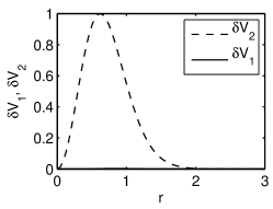
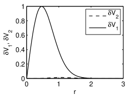
Figure 1: Internal modes ($m=3$) of the single charges vortex ($q=1$) with eigenvalue $\kappa=10.3$ (left) and the double charged vortex ($q=-2$) with eigenvalue $\kappa=9.1$ (right). $\delta V_{2}$ clearly dominates the nearly invisible $\delta V_{1}$ component in the left picture, whereas the opposite is the case in the right one.

       

       

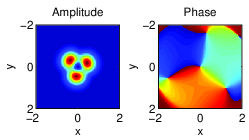
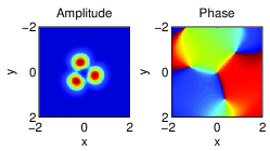
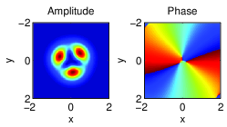
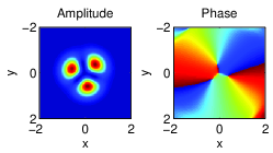
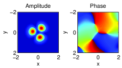
Figure 2: (First row) Tracking the family starting from the single charged vortex ($q=1$), the respective angular momenta and structural parameter are (from left to right) $L_{z}=450$, $\alpha=0.65$; $L_{z}=270$, $\alpha=0.53$; and $L_{z}=0$, $\alpha=0.4$. (Second row) Tracking the family starting from the double charged vortex ($q=-2$); $L_{z}=-1100$, $\alpha=0.55$; $L_{z}=-770$, $\alpha=0.3$; and $L_{z}=0$, $\alpha=0.4$ (from left to right).

From a topological point of view, the above findings are somehow surprising because the two limiting vortices have different charge ($q=1$ and $q=-2$). It is possible to understand this interesting feature when looking at the azimuthon close to the respective vortices. Starting from the double charged vortex ($q=-2$), the azimuthon is created by adding a counter-rotating single charged vortex ($m+q=1,$ see right panel in Fig. 1). However small the amplitude of this single charged vortex might be, in the vicinity of the origin it will always be dominant as it grows as $\sim r$, whereas the double charged vortex as $\sim r^{2}$. Thus, the azimuthon has a $q=1$ vorticity at the origin, and on a ring where the amplitudes of the two vortices are equal lie three phase singularities with charge $-1$ (see Fig. 3 for a schematic sketch). As we can see in Fig. 2, the radius of this ring grows when we follow the family of azimuthons towards the single charged vortex, and the three singularities with total charge $-3$ move far away from the origin and finally disappear when we approach the vortex with total charge $q=1$ (see discussion below). It is important to note that these three phase singularities have fixed positions with respect to the position of the three humps and follow the amplitude rotation of the azimuthon (co-rotating).

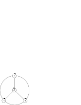
Figure 3: Sketch of the co-rotating topological charges observed in the azimuthon family of Fig. 2.

We will now discuss in a greater detail the three co-rotating phase singularities, in particular, how they disappear when we approach the vortex with total charge $q=1$. To this end, we analyze the asymptotic behavior for large $r$ of the three components of the azimuthon $V$, $\delta V_{1}$ and $\delta V_{2}$ [see Eq. (12)]. For sufficiently large $r$, the convolution term $\theta$ in Eqs. (1) and (11) can be neglected when compared to the term $\sim 1/r^{2}$ in the transverse Laplacian. Then, using the modified Bessel functions, one can find the asymptotic behavior of the involved functions easily:

$$\delta V_{1} \sim\frac{1}{\sqrt{r}}e^{-\sqrt{\kappa+\lambda_{0}}r}\left[1+\frac{4\left(m+q\right)^{2}-1}{8r\sqrt{\kappa+\lambda_{0}}}+\mathcal{O}\left(\frac{1}{r^{2}}\right)\right]$$ (13a)

$$\delta V_{2} \sim\frac{1}{\sqrt{r}}e^{-\sqrt{\lambda_{0}-\kappa}r}\left[1+\frac{4\left(m-q\right)^{2}-1}{8r\sqrt{\kappa+\lambda_{0}}}+\mathcal{O}\left(\frac{1}{r^{2}}\right)\right]$$ (13b)

$$V \sim\frac{1}{\sqrt{r}}e^{-\sqrt{\lambda_{0}}r}\left[1+\frac{4q^{2}-1}{8r\sqrt{\lambda_{0}}}+\mathcal{O}\left(\frac{1}{r^{2}}\right)\right].$$ (13c)

To find the radius $r_{s}$ where the phase singularities appear, one has to equal the amplitudes in the following manner:

$$\left|V\left(r\right)\right|=A_{r}\left|\delta V_{1}\left(r\right)+\delta V_{2}\left(r\right)\right|.$$ (14)

It is obvious from Eqs. (13a) that such a radius exists for arbitrary small $A_{r}$, because one of the $\delta V_{i}$ decays always slower than $V$ for $r\rightarrow\infty$. In our example we have $\kappa>0$, and therefore $\delta V_{2}$ is responsible for creating our three co-rotating phase singularities. For $A_{r}\rightarrow 0$ we find that $r_{s}\rightarrow\infty$, the singularities move to infinite distances form the origin and (formally) vanish for $A_{r}=0$. However, for practical observations in, e.g., numerical simulations those co-rotating phase singularities become irrelevant when the surrounding amplitude becomes small.

The observation that the above triple hump azimuthon has almost constant angular frequency when we follow the family for constant mass $M$ regime can be explained going over to the highly nonlocal limit. This rotation is not a purely nonlinear phenomenon, but is mainly a consequence of mode beating. Let us have a look at the related linear limit where we replace the nonlocal response $\Theta$ by the Gaussian kernel times mass $M$ (similar to Snyder-Mitchel model (Snyder and Mitchell, 1997)). In this linear problem we can find several eigenmodes (see Fig. 4). Mode beating between single ($q=1$) and double ($q=-2$) charged vortices predicts $\Omega\sim(\lambda_{G_{4}}-\lambda_{G_{2}})/3=-4.2$, which is not too far from the rotation frequency observed in the nonlocal nonlinear problem.

       

       

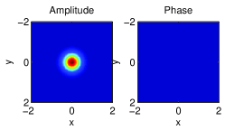
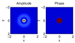
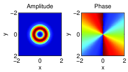
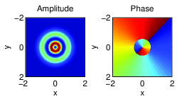
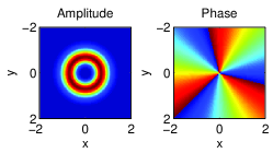
Figure 4: First six linear modes of a Gaussian potential with mass 630: Ground state $G_{1}(r)$, $\lambda_{G_{1}}=86.6$; single charged vortex $G_{2}(r)\exp(i\phi)$, $\lambda_{G_{2}}=73.5$; humped ring state $G_{3}(r)$, $\lambda_{G_{3}}=61.5$; double charged vortex $G_{4}(r)\exp(i2\phi)$, $\lambda_{G_{4}}=60.9$; single charged double ring $G_{5}(r)\exp(i\phi)$, $\lambda_{G_{5}}=50$; triple charged vortex $G_{6}(r)\exp(i3\phi)$, $\lambda_{G_{6}}=48.9$ (from left to right, top to down).

Another evidence that the linear contribution to the rotation of the triple hump dominates is that $|\Omega|$ increases strongly with mass $M$ (and $\lambda$), as expected from $\Omega\sim(\lambda_{G_{4}}-\lambda_{G_{2}})/3$. E.g., for $M=200$ we find $\Omega\sim-1.2$. In contrast to that, the double hump azimuthon connecting single charged vortex and stationary dipole shows almost no dependency of $\Omega$ on the mass (Skupin et al, 2008). This resembles the fact that in the linear problem mentioned above, mode beating predicts $\Omega\sim(\lambda_{G_{2}}-\lambda_{G_{2}})/2=0$ for this structure. In fact, following a reasoning similar to Buccoliero et al (2008), we can identify in the expression (7) for the rotation frequency a linear and nonlinear contribution, $\Omega=\Omega_{ln}+\Omega_{nln}$. In the limit $\Theta=M\exp(-r^{2}/2)/2\pi$ and $U$ a superposition of ”linear” modes we readily see that $MN^{\prime}-L_{z}N=0$, and any rotation is due to

$$\Omega_{ln}=\frac{MI^{\prime}-L_{z}I}{L_{z}^{2}-MM^{\prime}}.$$ (15)

In the special case that $U$ is a superposition of degenerated linear modes, we find $MI^{\prime}-L_{z}I=0$ and thus $\Omega_{ln}=0$. However, if we consider the original nonlinear system where $\Theta$ is given by Eq. (2), an additional (nonzero) nonlinear contribution

$$\Omega_{nln}=\frac{MN^{\prime}-L_{z}N}{L_{z}^{2}-MM^{\prime}}$$ (16)

to the rotation frequency occurs.

Once we have computed the internal mode of a vortex, we can construct all azimuthons branching from it. For example, Fig. 5 shows a rotating five-hump azimuthon emanating from our double charged vortex ($q=-2$). The corresponding internal mode shows a typical $~{}r^{(5-2)}$ dependence near the origin in $\delta V_{1}$, the amplitude of $\delta V_{2}$ is very small. Hence, for the azimuthon, we see the double charged phase singularity ($q=-2$) of the vortex in the origin. As observed for the rotatin triple-hump above, five singularities with $q=1$ appear on a ring, and they are expected to move inwards when we follow the azimuthon family towards the triple charged vortex with $q=3$.

   

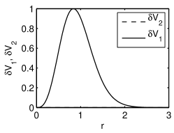
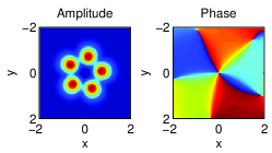
Figure 5: Internal mode ($m=5$) of the double charged vortex ($q=-2$) with eigenvalue $\kappa=-8.6$, and corresponding emanating azimuthon ($M=630$, $\alpha=0.56$). $\delta V_{1}$ clearly dominates the small $\delta V_{2}$ component in the left picture.

We can also easily identify families of azimuthons previously found using a special ansatz. For instance, the double charged vortex ($q=-2$) shows another internal mode for $m=2$ with eigenvalue $\kappa=-3.1$. As can be seen in Fig. 6, the resulting azimuthon belongs to the family connecting Hermite-Gaussian and Laguerre-Gaussian self-trapped modes HN₂₀ and LN₂₀ (Buccoliero et al, 2008). Note that for this solution our definition of the structural parameter $\alpha$ does not make sense, hence in the caption of Fig. 6 we give the rotation frequency $\Omega$ instead, to characterize the azimuthon.

   

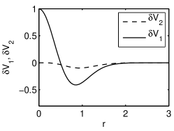
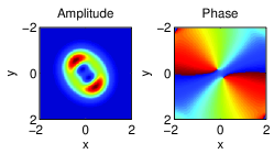
Figure 6: Internal mode ($m=2$) of the double charged vortex ($q=-2$) with eigenvalue $\kappa=3.1$, and corresponding emanating azimuthon ($M=630$, $\Omega=-1.44$).

Last but not least, we want to note here that the concept of azimuthons branching from solitons is not limited to vortices. E.g., the single-hump ground state ($M=630$, $q=0$) features a $m=2$ internal mode with $\kappa=-23.3$. The emanating azimuthon looks like a rotating bone, and possesses two phase singularities with opposite charges on an axis perpendicular to the ”bone” axis (see Fig. 7). The very high rotation frequency is again a manifestation of linear mode beating, we find $\Omega\sim(\lambda_{G_{1}}-\lambda_{G_{4}})/2=12.9$.

   

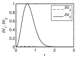
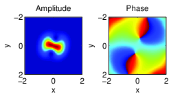
Figure 7: Internal mode ($m=2$) of the groundstate ($q=0$) with eigenvalue $\kappa=-23.3$, and corresponding emanating azimuthon ($M=630$, $\Omega=14.3$).

If we reduce mass and therefore, in our scaling, reduce nonlocality these results may change. First of all, solitons and azimuthons are expected to become unstable. Moreover, we observe that the second component of the perturbation becomes larger in amplitude when we leave the highly nonlocal regime (note that it is almost invisible in Figs. 1, 5, 5, and 7). Also, certain types of internal modes may vanish or new ones may appear. Hence, careful analysis of the internal spectra of soliton solutions is necessary to predict structure of azimuthons in a given regime or model, e.g., the local nonlinear Schrödinger equation.

5 Conclusion

In conclusion, we have demonstrated a simple method for identifying rotating solutions in nonlocal nonlinear media. We computed azimuthon solutions and their rotation frequencies numerically and showed that in the limit of minimal azimuthal amplitude modulation, i.e., close to a vortex soliton, the rotation frequency is determined uniquely by eigenvalues of the bound modes of the linearized version of the respective stationary nonlocal solution. Moreover, the intensity profile of the resulting azimuthons can be constructed from the corresponding linear eigensolution. This offers a straightforward and exhaustive method to identify rotating soliton solutions in a given nonlinear medium. At least, in the highly nonlocal regime, we find families of azimuthons which connect vortex solitons with different topological charge.