An energy-preserving Discrete Element Method for elastodynamics

Abstract

We develop a Discrete Element Method (DEM) for elastodynamics using polyhedral elements. We show that for a given choice of forces and torques, we recover the equations of linear elastodynamics in small deformations. Furthermore, the torques and forces derive from a potential energy, and thus the global equation is an Hamiltonian dynamics. The use of an explicit symplectic time integration scheme allows us to recover conservation of energy, and thus stability over long time simulations. These theoretical results are illustrated by numerical simulations of test cases involving large displacements.

000010

L. Monasse, C. MariottiAn energy-preserving D.E.M. for elastodynamics

Laurent Monasse, Université Paris-Est, CERMICS, 6 et 8 avenue Blaise Pascal, Cité Descartes – Champs-sur-Marne, 77455 Marne-la-Vallée Cedex 2, France

1 Introduction

Particle methods are meshless simulation techniques in which a continuum medium is approximated through the dynamics of a set of interacting particles. Two main classes of particle methods can be distinguished : Discrete Element methods (DEM), which rely on the contact interaction of material particles by means of forces and torques, and Smooth Particle Hydrodynamics (SPH) methods, in which the continuum is discretized by localized kernel functions.

Discrete Element methods consist in the resolution of the equations of motion of a set of particles submitted to forces and torques. It is thus possible to account for a variety of phenomena (behaviour laws, models, scales,…) using a single numerical method. A wide variety of Discrete Elment methods have been designed changing the expression of the forces, with particular attention devoted to specific aspects. Discrete Element methods have first been developed by Hoover, Arhurst and Olness [20] in models for crystalline materials. Their application to geotechnical problems was carried out by Cundall and Strack [4], and their use in granular materials and rock simulation is still widespread [37, 36]. Discrete Element Methods have also been used to simulate thermal conduction in granular assemblies [10] or fluid-structure interaction [16]. The model is also able to account for grain size effects [21], and to treat fracture in a natural way. Discrete Element methods used for granular materials generally describe particles as spherical elements interacting via noncohesive, frictional contact forces [37]. For brittle materials, models also use unilateral contact forces, combined with bonds which simulate cohesion [36]. Kun and Herrmann developed a combination of the contact model with a lattice model of beams to account for the cohesion [26], which has been extended to Reissner models of beams to simulate large rotations of the material [5, 21]. The authors use Voronoi tesselations to generate the polygonal particles. However, the results obtained still depend on the size of the discretization (which physically corresponds to the size of heterogeneities) [21]. The effective macroscopic Young modulus and Poisson ratio highly depend on the isotropy of the distribution of the particles and are only empirically linked to their microscopic value for the Reissner beams [26].

In a different approach, SPH methods describe the particles as smooth density kernel functions. The kernel functions are an approximation of the partition of unity. The continuous equations of evolution of the fluid or solid material therefore induce the dynamics of the particles. Originating from astrophysical compressible fluid simulations [12, 33], SPH was extended to incompressible fluids [35] and to elastic and plastic dynamics [32], and used for fluid-structure interaction with both domains discretized with SPH [2]. A state of the art review of the method with applications to solid mechanics is presented in [19]. SPH preserves the total mass of the system exactly. However, in tensile regime, unphysical clusters of particles tend to appear in situations where a homogeneous response is expected [40]. Hicks, Swegle and Attaway advocate the smoothing of the variables between neighbouring particles to stabilize the method, rather than introducing artificial viscosities [18]. Bonet and Lok have addressed the issue of angular momentum preservation, and show that rotational invariance is equivalent to the exact evaluation of the gradients of linear velocity fields, which can be achieved either through correction of the kernel function or through a modification of its gradient [3]. In order to circumvent the difficulties affecting SPH, Yserentant developed the Finite Mass method, in which particles of fixed size and shape also possess a rotational degree of freedom (spin). The method achieves effective partition of unity, and thus preserves momentum, angular momentum and energy, ensuring stability [42].

The Moving Particle Semi-implicit (MPS) method is a variant of the SPH method developed by Koshizuka. It consists in the derivation of the dynamics of a set of points from a discrete Hamiltonian [23]. As in the SPH method, the differential operators are approximated by a kernel function of compact support. The expression of the approximated differential operators is inserted in the classical Hamiltonian of the system, and by application of Hamilton’s equations, the dynamics of the discretized system is obtained. To preserve the Hamiltonian structure of the dynamic of the system through time discretization, the authors use symplectic schemes [39]. The MPS method has been used initially for free-surface flows [23, 24], and has been extended to nonlinear elastodynamics [25, 39] and to fluid-structure interaction [29]. Using similar ideas, by deriving the dynamics of the system from a discrete Hamiltonian, Fahrenthold has simulated compressible flows [22] and impact events with breaking of the target [8, 9].

These methods show the importance of the preservation of momentum and energy for the accuracy and stability of the scheme over long-time simulation. The use of symplectic schemes ensures the preservation of the structure of Hamilton’s equations by the numerical time integration, and therefore the preservation of momentum and energy [15]. Simo, Tarnow and Wong note, however, that while ensuring the stability of the simulation for small time steps, the symplectic schemes fail to preserve exactly energy and become unstable for larger time steps [38]. They derive a general class of implicit time-stepping algorithms which exactly enforce the conservation of momentum, angular momentum and energy. The algorithms are built in order to preserve linear and angular momentum, and energy conservation is enforced either with a projection method (projection on the manifold of constant energy) or with a collocation method. The algorithm is used for nonlinear elasticity in large deformation using finite element methods [38, 13, 28] and for low-velocity impact [17].

In this article, we extend and analyze the Discrete Element method initially introduced by Mariotti [34]. Combining a Discrete Element Method with a lattice model of beams, we are able to account for the cohesion of the material, and analytically recover the macroscopic behaviour of the continuous material. The method, Mka3D, has been successfully used to simulate the propagation of seismic waves in linear elastic medium [34]. Here, we extend the properties of the algorithm to the case of large displacements without fracture. Contrary to usual Discrete Element methods, we are able to derive the microscale forces and torques analytically from the macroscopic Young modulus and Poisson ratio, and to prove the convergence of the method as the grid is refined. In addition, as in MPS methods, we derive the forces and torques between particles from a Hamiltonian formulation. Using a symplectic scheme, we ensure the preservation of energy over long-time simulations, and thus stability of the method. This allows for the simulation of three-dimensional wave propagation as well as shell or multibody dynamics. The paper is organized as follows. In section 2, we describe the lattice model used. We introduce the Hamiltonian of the system and we derive the expression of forces and torques chosen to simulate linear elasticity. In section 3, we show that these expressions lead to a macroscopic behaviour of the material equivalent to a Cosserat continuum, with a characteristic length of the order of the size of the particles. Hence, the model is consistent with a Cauchy continuum medium up to second-order accuracy, in the case of small displacement and small deformation. The microscopic values of Young modulus and Poisson ratio yield directly the macroscopic values, and we can choose Poisson ratio in the whole interval $(-1,0.5)$. In section 4, we then describe the symplectic RATTLE time-scheme [15], which allows us to preserve a discrete energy over long-time simulations. These theoretical results are illustrated by numerical simulations of test cases involving large displacements in section 5.

2 Description of the method

2.1 Geometrical description of the system

In order to discretize the continuum material, several methods have been suggested for Discrete Element Methods. Most authors working on granular materials use hard spheres, in order to simplify the computation of contacts between particles, as the exact form of the particles is mainly unknown. However, in the case of the simulation of a continuous material, this method is not adapted as the interstitial vacuum between spheres is inconsistent with the compactness of the solid. In addition, the difficulty to obtain a dense packing of hard spheres, and the problem of the expression of cohesion between the particles, have led us to use Voronoi tesselations instead, as suggested in [26, 5]. The particles are therefore convex polyhedra which define a partition of the entire domain. As we shall see, this method allows us to handle any Poisson ratio $\nu$ strictly between $-1$ and $0.5$, independently from the size of the particles. On the contrary, most granular sphere packing methodologies account for a limited range of $\nu$, which is size dependent.

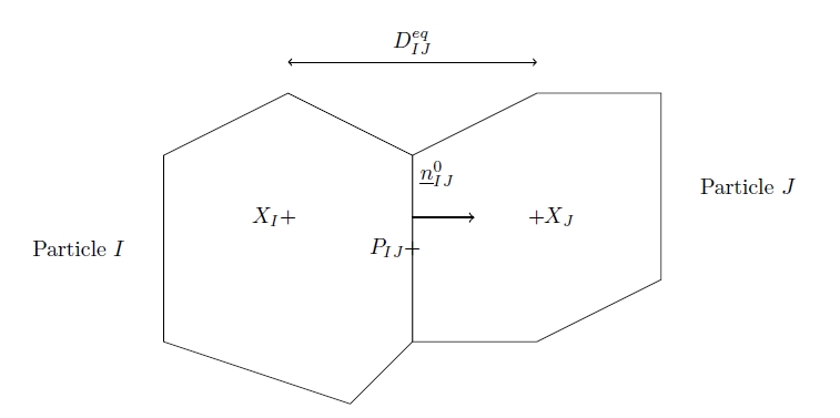
Figure 1: Geometric description of the particles

The following parameters are relevant to describe the motion of a given particle $I$ : $\underline{X}_{I}$ and $\underline{v}_{I}$ denote respectively the position and velocity of its center of mass ($\underline{v}_{I}=\frac{d\underline{X}_{I}}{dt}$), $\underline{\underline{Q}}_{I}$ denotes the orthogonal rotation matrix of the frame attached to the rigid particle, and the angular velocity vector $\underline{\Omega}_{I}$ is uniquely defined by :

$$\underline{\underline{j}}(\underline{\Omega}_{I})=\frac{d\underline{\underline{Q}}_{I}}{dt}\underline{\underline{Q}}_{I}^{T},$$ (1)

where the map $\underline{\underline{j}}:\mathbb{R}^{3}\rightarrow\mathbb{R}^{3\times 3}$ is such that :

$$\forall\underline{x}\in\mathbb{R}^{3},\;\forall\underline{y}\in\mathbb{R}^{3},\;\underline{\underline{j}}(\underline{x})\cdot\underline{y}=\underline{x}\wedge\underline{y}$$

Finally, the material of particle $I$ is described by its mass $m_{I}$, its volume $V_{I}$ and its principal moments of inertia $I_{I}^{1}$, $I_{I}^{2}$ and $I_{I}^{3}$. We suppose the local frame attached to the particle is attached to the principal axes of inertia $(\underline{e}^{1}_{I},\underline{e}^{2}_{I},\underline{e}^{3}_{I})$. The matrix of inertia in the fixed frame is given by :

$$\underline{\underline{R}}_{I}=\underline{\underline{Q}}_{I}\cdot\underline{\underline{R}}_{I}^{0}\cdot\underline{\underline{Q}}_{I}^{-1}$$ (2)

where $\underline{\underline{R}}_{I}^{0}$ is the matrix of inertia $\underline{\underline{R}}_{I}^{0}$ written in the inertial frame :

$$\underline{\underline{R}}_{I}^{0}=\left(\begin{array}[]{ccc}I_{I}^{1}&0&0\\ 0&I_{I}^{2}&0\\ 0&0&I_{I}^{3}\end{array}\right)$$

We also define the parameters $d_{I}^{1}$, $d_{I}^{2}$ and $d_{I}^{3}$ as :

$$d_{I}^{i}=\frac{I_{I}^{1}+I_{I}^{2}+I_{I}^{3}}{2}-I_{I}^{i},\quad i=1,2,3$$

and we introduce the following matrix $\underline{\underline{D}}_{I}$ defined in the inertial frame :

$$\underline{\underline{D}}_{I}=\left(\begin{array}[]{ccc}d_{I}^{1}&0&0\\ 0&d_{I}^{2}&0\\ 0&0&d_{I}^{3}\end{array}\right)$$

The Discrete Element Method relies on the computation of forces and torques between nearest neighbours particles. We denote by $\mathcal{V}_{I}$ the list of the neighbouring particles linked to particle $I$. For each link between two particles $I$ and $J$, we define $P_{IJ}$ the center of mass of the interface, $S_{IJ}$ the surface of the interface, the distance between particles $I$ and $J$ :

$$D_{IJ}=\lVert\underline{X_{I}X_{J}}\rVert,$$

and the initial exterior normal vector for link $IJ$ :

$$\underline{n}_{IJ}=\frac{1}{D_{IJ}}\underline{X_{I}X_{J}}$$

We define two normalized orthogonal vectors of the interface $\underline{s}_{IJ}$ and $\underline{t}_{IJ}=\underline{n}_{IJ}\wedge\underline{s}_{IJ}$, serving as references to evaluate the torsion between particles $I$ and $J$.

These parameters are given a fixed value at the beginning of the computation. $D_{IJ}^{0}$ and $\underline{n}_{IJ}^{0}$ respectively denote the initial values for $D_{IJ}$ and $\underline{n}_{IJ}$. The particles are therefore assumed to be rigid. However, compressibility effects are taken into account through the expression of interaction potentials.

In addition, we define the following quantities :

• the displacement at the interface between particles $I$ and $J$ :

  $$\underline{\Delta u}_{IJ}=\underline{X_{J}}-\underline{X_{I}}+\underline{\underline{Q}}_{J}\cdot\underline{X_{J}^{0}P_{IJ}}-\underline{\underline{Q}}_{I}\cdot\underline{X_{I}^{0}P_{IJ}}$$

• When particle $I$ has several free interfaces (i.e. not linked to another particle), these surfaces are marked as stress-free. To account for the free deformation of the particle in these directions, free-volume $V_{I}^{l}$ is defined as the sum of the volumes of all pyramidal polyhedra with a free surface as basis and $X_{I}^{0}$ as summit.

• the volumetric deformation $\varepsilon_{I}^{v}$ of particle $I$  is defined as the sum of all contributions of the deformations of the material links of particle $I$. We have assumed that the bending of the link between two particles does not affect volume, as long as the centers of the interface of the two particles stay in contact. The corrective term on the volume is active only on particles having a free surface, and accounts for the boundary condition $\underline{\underline{\sigma}}\cdot\underline{n}=\underline{0}$. We derive it in Appendix A.

  $$\varepsilon_{I}^{v}=\sum_{J\in\mathcal{V}_{I}}{\frac{1}{2}\frac{S_{IJ}}{V_{I}+3\frac{\nu}{1-2\nu}V_{I}^{l}}\underline{\Delta u}_{IJ}\cdot\underline{n}_{IJ}}$$

• The interpolated volumetric deformation for link $(IJ)$ :

  $$\varepsilon_{IJ}^{v}=\frac{1}{2}(\varepsilon_{I}^{v}+\varepsilon_{J}^{v})$$

2.2 Expression of the Hamiltonian of the system

We denote by $E$ the Young’s modulus and by $\nu$ the Poisson’s ratio for the material. The Hamiltonian formulation of the elastodynamic equations on a domain $\Omega$ is as follows :

$$H(\underline{q},\underline{p})=\int_{\Omega}{\frac{1}{2\rho}\underline{p}\cdot\underline{p}}+U(\underline{q})$$ (3)

where $\underline{q}$ is the displacement field and $\underline{p}=\rho\underline{v}$ is the density of momentum. $U(\underline{q})$ is the potential energy of the system. It can be expressed in terms of the stress tensor $\underline{\underline{\sigma}}$ and the linearized strain tensor $\underline{\underline{\varepsilon}}=\frac{1}{2}(\underline{\underline{\nabla}}\underline{q}+{\underline{\underline{\nabla}}\underline{q}}^{\text{T}})$ :

$$U(\underline{q})=W(\underline{\underline{\varepsilon}})=\frac{1}{2}\int_{\Omega}{\underline{\underline{\sigma}}(\underline{\underline{\varepsilon}}):\underline{\underline{\varepsilon}}}$$ (4)

In the case of Cauchy linear elasticity, we use the constitutive relation

$$\underline{\underline{\sigma}}(\underline{\underline{\varepsilon}})=\frac{E}{1+\nu}\underline{\underline{\varepsilon}}+\frac{E\nu}{(1+\nu)(1-2\nu)}\text{tr~{}}(\underline{\underline{\varepsilon}})\underline{\underline{Id}}$$ (5)

to derive the expressions of $W(\varepsilon)$ and $U(\underline{q})$ :

$$W(\underline{\underline{\varepsilon}})=\frac{1}{2}\int_{\Omega}{\frac{E}{1+\nu}\underline{\underline{\varepsilon}}:\underline{\underline{\varepsilon}}+\frac{E\nu}{(1+\nu)(1-2\nu)}\text{tr~{}}(\underline{\underline{\varepsilon}})^{2}}$$ (6)

$$U(\underline{q})=\frac{1}{2}\int_{\Omega}{\frac{E}{2(1+\nu)}\underline{\underline{\nabla}}\underline{q}:\underline{\underline{\nabla}}\underline{q}+\frac{E}{2(1+\nu)(1-2\nu)}(\text{div}\text{~{}}\underline{q})^{2}}$$ (7)

We choose to discretize the Hamiltonian formulation as a discrete Hamiltonian $H_{h}$. The displacement field $\underline{q}$ is derived from the values of $(\underline{X}_{I},\underline{\underline{Q}}_{I})$. The density of momentum derives from :

$$\underline{T}_{I} =m_{I}\underline{v}_{I}$$ (8)

$$\underline{\underline{P}}_{I} =\underline{\underline{j}}(\underline{\Omega}_{I})\cdot\underline{\underline{Q}}_{I}\cdot\underline{\underline{D}}_{I}$$ (9)

We define :

$$H_{h}(\underline{X},\underline{\underline{Q}},\underline{T},\underline{\underline{P}})=\frac{1}{2}\sum_{I}{\frac{1}{m_{I}}\underline{T}_{I}\cdot\underline{T}_{I}}+\frac{1}{2}\sum_{I}{\text{tr~{}}(\underline{\underline{P}}_{I}\cdot\underline{\underline{D}}_{I}^{-1}\cdot{\underline{\underline{P}}_{I}}^{\text{T}})}+U_{h}(\underline{X},\underline{\underline{Q}})$$ (10)

The discretized potential energy is split into three terms :

$$U_{h}(\underline{X},\underline{\underline{Q}})=U_{t}(\underline{X},\underline{\underline{Q}})+U_{d}(\underline{X},\underline{\underline{Q}})+U_{f}(\underline{\underline{Q}})$$

$U_{t}(\underline{X},\underline{\underline{Q}})$ corresponds to the first term of (6) : we approach the strain of the link $(IJ)$ in the direction $\underline{n}_{IJ}$ $\underline{\underline{\varepsilon}}\cdot\underline{n}_{IJ}$ by the normalized displacement $\frac{1}{D_{IJ}^{0}}\underline{\Delta u}_{IJ}$, and we use the approximation :

$$\underline{\underline{\varepsilon}}:\underline{\underline{\varepsilon}}\approx\sum_{J\in\mathcal{V}_{I}}{(\underline{\underline{\varepsilon}}\cdot\underline{n}_{IJ})^{2}}$$ (11)

We therefore write :

$$U_{t}(\underline{X},\underline{\underline{Q}})=\frac{1}{2}\sum_{(IJ)}{S_{IJ}\frac{E}{1+\nu}\frac{\underline{\Delta u}_{IJ}\cdot\underline{\Delta u}_{IJ}}{D_{IJ}^{0}}}$$

This energy accounts for the deformation of each link between two particles.

$U_{d}(\underline{X},\underline{\underline{Q}})$ corresponds to the second term of (6) : we approach the trace of the strain $\text{tr}(\underline{\underline{\varepsilon}})$ in particle $I$ by the sum of the normalized displacements $\varepsilon_{I}^{v}$ for links surrounding $I$. A corrective term is added for cells having a free boundary :

$$U_{d}(\underline{X},\underline{\underline{Q}})=\frac{1}{2}\sum_{I}{\frac{E\nu}{(1+\nu)(1-2\nu)}(V_{I}+3\frac{\nu}{1-2\nu}V_{I}^{l})(\varepsilon_{I}^{v})^{2}}$$

This energy accounts for the global volumetric deformation of each particle.

The former two terms are sufficient to recover the equations of elastodynamics inside the solid. However, for the method to be able to cope with thin one-element shells, we add the pure flexion term $U_{f}(\underline{\underline{Q}})$ :

$$U_{f}(\underline{\underline{Q}})=-\sum_{(IJ)}{\frac{S_{IJ}}{D_{IJ}^{0}}\left(\alpha_{n}(\underline{\underline{Q}}_{J}\cdot\underline{n}_{IJ}^{0})\cdot(\underline{\underline{Q}}_{I}\cdot\underline{n}_{IJ}^{0})\right.}\left.+\alpha_{s}(\underline{\underline{Q}}_{J}\cdot\underline{s}_{IJ})\cdot(\underline{\underline{Q}}_{I}\cdot\underline{s}_{IJ})+\alpha_{t}(\underline{\underline{Q}}_{J}\cdot\underline{t}_{IJ})\cdot(\underline{\underline{Q}}_{I}\cdot\underline{t}_{IJ})\right)$$

This term accounts for the flexion between particles. The coefficients $\alpha_{n}$, $\alpha_{s}$ and $\alpha_{t}$ are chosen to recover the exact flexion and torsion of a beam, and are detailed in Appendix B.

2.3 Derivation of the forces and torques between particles

We use Hamilton’s equations for the system (10) :

$$\underline{\dot{X}}_{I} =\frac{\partial H_{h}}{\partial\underline{T}_{I}}$$ (12)

$$\underline{\underline{\dot{Q}}}_{I} =\frac{\partial H_{h}}{\partial\underline{\underline{P}}_{I}}$$ (13)

$$\underline{\dot{T}}_{I} =-\frac{\partial H_{h}}{\partial\underline{X}_{I}}$$ (14)

$$\underline{\underline{\dot{P}}}_{I} =-\frac{\partial H_{h}}{\partial\underline{\underline{Q}}_{I}}+\underline{\underline{\Lambda}}_{I}\cdot\underline{\underline{Q}}_{I}$$ (15)

where $\underline{\underline{\Lambda}}_{I}$ is the symmetric matrix of the Lagrange multipliers associated with the constraint ${\underline{\underline{Q}}_{I}}^{\text{T}}\cdot\underline{\underline{Q}}_{I}=\underline{\underline{Id}}$.

Equations (12) and (13) give us the usual kinematic relations between position and velocity :

$$\underline{\dot{X}}_{I} =m_{I}^{-1}\underline{T}_{I}=\underline{v}_{I}$$

$$\underline{\underline{\dot{Q}}}_{I} =\underline{\underline{P}}_{I}\cdot\underline{\underline{D}}_{I}^{-1}=\underline{\underline{j}}(\underline{\Omega}_{I})\cdot\underline{\underline{Q}}_{I}$$

The derivation of forces and torques from the potential energies is carried out in Appendix C. We obtain $m_{I}\underline{\dot{v}}_{I}=\underline{F}_{IJ}$ where $\underline{F}_{IJ}$, the force exerted by particle $I$ on particle $J$, is given by :

$$\underline{F}_{IJ}=\frac{S_{IJ}}{D_{IJ}^{0}}\frac{E}{1+\nu}\underline{\Delta u}_{IJ}+S_{IJ}\frac{E\nu}{(1+\nu)(1-2\nu)}\varepsilon_{IJ}^{v}\left(\underline{n}_{IJ}+\frac{1}{D_{IJ}}\underline{\Delta u}_{IJ}-\frac{1}{D_{IJ}}(\underline{\Delta u}_{IJ}\cdot\underline{n}_{IJ})\underline{n}_{IJ}\right)$$ (16)

This expression can be seen as a discrete version of Hooke’s law of linear elasticity

$$\underline{\underline{\sigma}}=\frac{E}{1+\nu}\underline{\underline{\varepsilon}}+\frac{E\nu}{(1+\nu)(1-2\nu)}\text{tr}(\underline{\underline{\varepsilon}})\underline{\underline{Id}}$$ (17)

using the previous analogies between $\frac{1}{D_{IJ}^{0}}\underline{\Delta u}_{IJ}$ and $\underline{\underline{\varepsilon}}$, $\varepsilon_{IJ}^{v}$ and $\text{tr~{}}\underline{\underline{\varepsilon}}$, and noting that $\underline{\underline{\sigma}}\cdot\underline{n}$ is a force per surface unit (a pressure).

For the rotational part, we define the two following torques :

$$\underline{M}_{IJ}^{t}=\frac{S_{IJ}}{D_{IJ}^{0}}\frac{E}{1+\nu}(\underline{\underline{Q}}_{I}\cdot\underline{X_{I}^{0}P_{IJ}})\wedge\underline{\Delta u}_{IJ}+\frac{E\nu}{(1+\nu)(1-2\nu)}\varepsilon_{IJ}^{v}S_{IJ}(\underline{\underline{Q}}_{I}\cdot\underline{X_{I}^{0}P_{IJ}})\wedge\underline{n}_{IJ}$$ (18)

$$\underline{M}_{IJ}^{f}=\frac{S_{IJ}}{D_{IJ}^{0}}\left(\alpha_{n}(\underline{\underline{Q}}_{I}\cdot\underline{n}_{IJ}^{0})\wedge(\underline{\underline{Q}}_{J}\cdot\underline{n}_{IJ}^{0})\right.\left.+\alpha_{s}(\underline{\underline{Q}}_{I}\cdot\underline{s}_{IJ})\wedge(\underline{\underline{Q}}_{J}\cdot\underline{s}_{IJ})\right.\left.+\alpha_{t}(\underline{\underline{Q}}_{I}\cdot\underline{t}_{IJ})\wedge(\underline{\underline{Q}}_{J}\cdot\underline{t}_{IJ})\right)$$ (19)

We note the fact that $\underline{M}_{IJ}^{t}$ corresponds to the torque at the center of mass of the force $\underline{F}_{IJ}$ exerted by particle $J$ on particle $I$ at point $P_{IJ}$ :

$$\underline{M}_{IJ}^{t}=(\underline{\underline{Q}}_{I}\cdot\underline{X_{I}^{0}P_{IJ}})\wedge\underline{F}_{IJ}$$

and $\underline{M}_{IJ}^{f}$ is the flexion-torsion torque. We get the equation on the angular velocity :

$$\frac{d}{dt}\left(\underline{\underline{R}}_{I}\cdot\underline{\Omega}_{I}\right)=\sum_{J\in\mathcal{V}_{I}}{\underline{M}_{IJ}^{t}+\underline{M}_{IJ}^{f}}$$ (20)

In the case when exterior forces and torques are applied to the system, they are to be added to the internal forces and torques computed above.

3 Consistency and accuracy of the scheme

In this section, we investigate the consistency and the accuracy of the scheme. We first propose a modified equation for small displacements and small deformations. As the equations obtained are coupled dynamics for displacement and rotation, we compare the model with Cosserat generalized continuum, and recover a Cauchy continuum as the spatial discretization $h$ tends to zero.

3.1 Modified equation for the scheme

The modified equation approach is a standard scheme analysis where a set of continuous equations verified by the approximate solution is seeked for. These modified equations should be an approximate version of continuous equations derived from physics.

In order to be able to carry out a Taylor developments of the displacement, we place the points of the Voronoi tesselation on a Cartesian grid. The Discrete Element method can be seen, in this simplified case, as a Finite Difference scheme.

We assume that no exterior force and no exterior torque are applied on the system. The displacement $\underline{\xi}_{I}$ of particle $I$ is given by :

$$\underline{\xi}_{I}=\underline{X}_{I}-\underline{X}_{I}^{0}$$

We assume that $\underline{\xi}$ is a regular function on the domain, and we can therefore expand $\underline{\xi}_{J}$ at point $I$ with Taylor series if $J\in\mathcal{V}_{I}$. We denote $\Delta x$, $\Delta y$ and $\Delta z$ the grid steps in each direction, and $h$ their maximum.

We assume displacements and rotations to be small. We denote $\theta_{x}^{I}$, $\theta_{y}^{I}$ and $\theta_{z}^{I}$ the small rotation angles around axes $x$, $y$ and $z$.

Using (16), a simple Taylor development of the equations of motion yields for the displacement :

$$\rho\ddot{\xi}_{x}=\frac{E}{1+\nu}\left(\frac{\partial^{2}\xi_{x}}{\partial x^{2}}+\frac{\partial^{2}\xi_{x}}{\partial y^{2}}+\frac{\partial^{2}\xi_{x}}{\partial z^{2}}+\frac{\partial\theta_{z}}{\partial y}-\frac{\partial\theta_{y}}{\partial z}\right)+\frac{E\nu}{(1+\nu)(1-2\nu)}\left(\frac{\partial^{2}\xi_{x}}{\partial x^{2}}+\frac{\partial^{2}\xi_{y}}{\partial x\partial y}+\frac{\partial^{2}\xi_{z}}{\partial x\partial z}\right)\\ +\frac{E}{1+\nu}\left(\frac{\Delta x^{2}}{12}\frac{\partial^{4}\xi_{x}}{\partial x^{4}}+\frac{\Delta y^{2}}{12}\frac{\partial^{4}\xi_{x}}{\partial y^{4}}\right.\left.+\frac{\Delta z^{2}}{12}\frac{\partial^{4}\xi_{x}}{\partial z^{4}}+\frac{\Delta y^{2}}{6}\frac{\partial^{3}\theta_{z}}{\partial y^{3}}-\frac{\Delta z^{2}}{6}\frac{\partial^{3}\theta_{y}}{\partial z^{3}}\right)\\ +\frac{E\nu}{(1+\nu)(1-2\nu)}\left(\frac{\Delta x^{2}}{3}\frac{\partial^{4}\xi_{x}}{\partial x^{4}}+\frac{\Delta x^{2}}{6}\frac{\partial^{4}\xi_{y}}{\partial x^{3}\partial y}\right.\left.+\frac{\Delta x^{2}}{6}\frac{\partial^{4}\xi_{z}}{\partial x^{3}\partial z}+\frac{\Delta y^{2}}{6}\frac{\partial^{4}\xi_{y}}{\partial x\partial y^{3}}+\frac{\Delta z^{2}}{6}\frac{\partial^{4}\xi_{z}}{\partial x\partial z^{3}}\right)\\ +\mathcal{O}(h^{3})$$ (21)

The same results hold for $\xi_{y}$ and $\xi_{z}$ permuting the indices $x$, $y$ and $z$ circularly.

Using (18) and (19), (20) gives the equivalent equation for the rotation :

$$\frac{\Delta y^{2}+\Delta z^{2}}{12}\rho\ddot{\theta}_{x}=\frac{E}{1+\nu}\left(\frac{\partial\xi_{z}}{\partial y}-\frac{\partial\xi_{y}}{\partial z}-2\theta_{x}\right.\left.+\frac{\Delta y^{2}}{6}\frac{\partial^{3}\xi_{z}}{\partial y^{3}}-\frac{\Delta z^{2}}{6}\frac{\partial^{3}\xi_{y}}{\partial z^{3}}+\frac{\Delta y^{4}}{120}\frac{\partial^{5}\xi_{z}}{\partial y^{5}}\right.\\ \left.-\frac{\Delta z^{4}}{120}\frac{\partial^{5}\xi_{y}}{\partial z^{5}}-\frac{\Delta y^{2}}{4}\frac{\partial^{2}\theta_{x}}{\partial y^{2}}-\frac{\Delta z^{2}}{4}\frac{\partial^{2}\theta_{x}}{\partial z^{2}}\right.\left.-\frac{\Delta y^{4}}{48}\frac{\partial^{4}\theta_{x}}{\partial y^{4}}-\frac{\Delta z^{4}}{48}\frac{\partial^{4}\theta_{x}}{\partial z^{4}}\right)\\ +E\left[\frac{\Delta y^{2}+\Delta z^{2}}{12(1+\nu)}\left(\frac{\partial^{2}\theta_{x}}{\partial x^{2}}+\frac{\Delta x^{2}}{12}\frac{\partial^{4}\theta_{x}}{\partial x^{4}}\right)\right.\left.+\frac{\Delta z^{2}}{12}\left(\frac{\partial^{2}\theta_{x}}{\partial y^{2}}+\frac{\Delta y^{2}}{12}\frac{\partial^{4}\theta_{x}}{\partial y^{4}}\right)\right.\\ \left.+\frac{\Delta y^{2}}{12}\left(\frac{\partial^{2}\theta_{x}}{\partial z^{2}}+\frac{\Delta z^{2}}{12}\frac{\partial^{4}\theta_{x}}{\partial z^{4}}\right)\right]+\mathcal{O}(h^{5})$$ (22)

The same results hold for $\theta_{y}$ and $\theta_{z}$ permuting the indices $x$, $y$ and $z$ circularly.

We see that these sets of equations couple $\underline{\xi}$ and $\underline{\theta}$, and by construction of the method, no constitutive law exists between $\underline{\xi}$ and $\underline{\theta}$. The fact that a rotation remains in the equations can be compared to Cosserat continuum theory. We investigate this comparison in the following subsection.

3.2 Comparison with Cosserat and Cauchy continuum theories

In a Cosserat model for continuum media, the kinematics is described by a displacement field $\underline{u}$ and a rotation field $\underline{\phi}$. A modified strain tensor $\underline{\underline{\varepsilon}}$ and a new curvature strain tensor $\underline{\underline{\kappa}}$ are introduced [7] :

$$\underline{\underline{\varepsilon}} =\underline{\underline{\nabla}}\underline{u}+\underline{\underline{j}}(\underline{\phi})$$

$$\underline{\underline{\kappa}} =\underline{\underline{\nabla}}\underline{\phi}$$

We define $\underline{\underline{t}}$ and $\underline{\underline{\mu}}$ the stress and couple stress tensors. We assume the following constitutive relations :

$$\underline{\underline{t}} =\lambda\text{tr~{}}(\underline{\underline{\varepsilon}})\underline{\underline{Id}}+\mu\underline{\underline{\varepsilon}}+\mu_{c}\underline{\underline{\varepsilon}}^{\text{T}}$$ (23)

$$\underline{\underline{\mu}} =\alpha\text{tr~{}}(\underline{\underline{\kappa}})\underline{\underline{Id}}+\gamma\underline{\underline{\kappa}}+\beta\underline{\underline{\kappa}}^{\text{T}}$$ (24)

where $\lambda$, $\mu$, $\mu_{c}$, $\alpha$, $\beta$ and $\gamma$ are elastic moduli.

The dynamical equations for the system are :

$$\rho\underline{\ddot{u}} =\underline{\text{div}}\text{~{}}\underline{\underline{t}}$$

$$\underline{\underline{I}}_{c}\underline{\ddot{\phi}} =\underline{\text{div}}\text{~{}}\underline{\underline{\mu}}+\underline{\underline{\underline{e}}}:\underline{\underline{t}}$$

where $\rho$ denotes the density, $\underline{\underline{I}}_{c}$ is a characteristic inertia matrix, $:$ denotes the double contraction product of tensors, and $\underline{\underline{\underline{e}}}$ is defined as follows :

$$(\underline{\underline{\underline{e}}})_{ijk}=\left\{\begin{array}[]{ll}1&\text{if $(ijk)$ is an even permutation}\\ -1&\text{if $(ijk)$ is an odd permutation}\\ 0&\text{otherwise}\end{array}\right.$$

Using the constitutive relations (23) and (24), the following equations can be obtained :

$$\rho\underline{\ddot{u}} =(\lambda+\mu_{c})\underline{\nabla}\text{div}\text{~{}}\underline{u}+\mu\Delta\underline{u}+(\mu-\mu_{c})\underline{\text{curl}}\text{~{}}\underline{\phi}$$ (25)

$$\underline{\underline{I}}_{c}\underline{\ddot{\phi}} =(\alpha+\beta)\underline{\nabla}\text{div}\text{~{}}\underline{\phi}+\gamma\Delta\underline{\phi}-2(\mu-\mu_{c})\underline{\phi}+(\mu-\mu_{c})\underline{\text{curl}}\text{~{}}\underline{u}$$ (26)

Identifying the terms of (25) with equation (21), we find :

$$\lambda =\frac{E\nu}{(1+\nu)(1-2\nu)}$$

$$\mu =\frac{E}{1+\nu}$$

$$\mu_{c} =0$$

and we therefore recover the classical expression, for Cauchy media, of the first Lamé coefficient $\lambda_{Cauchy}$, and $\frac{\mu+\mu_{c}}{2}$ corresponds to the classical second Lamé coefficient $\mu_{Cauchy}$. Comparing then equation (26) with equation (22), we find :

$$\underline{\underline{I}}_{c}=\rho\left(\begin{array}[]{ccc}\frac{\Delta y^{2}+\Delta z^{2}}{12}&0&0\\ 0&\frac{\Delta x^{2}+\Delta z^{2}}{12}&0\\ 0&0&\frac{\Delta x^{2}+\Delta y^{2}}{12}\end{array}\right)$$

For a given $h=\Delta x=\Delta y=\Delta z$, we see that the modified equations for the scheme are those of a Cosserat generalized continuum, with second-order accuracy, and the coefficients verify $\alpha+\beta=0$ and $\gamma=\frac{E}{2(1+\nu)}h^{2}$. In the case of an anisotropic mesh size ($\Delta x\neq\Delta y\neq\Delta z$), we cannot identify the coefficients with the isotropic Cosserat equations, due to the presence of the Laplacian operator. We can however find an anisotropic Cosserat model with weighted second derivatives instead of the Laplacian.

One of the main characteristics of a Cosserat generalized continuum is to exhibit a characteristic length for the material, $l_{c}$, which describes the length of the nonlocal interactions. $l_{c}$ is defined as :

$$l_{c}^{2}=\frac{\gamma}{\mu+\mu_{c}}$$

In our case, we see that :

$$l_{c}=\frac{\sqrt{2}}{2}h$$

$l_{c}$ is of the same order as the size of the particles. In an homogenization analysis framework, S. Forest, F. Pradel and K. Sab have shown [11] that when the macroscopic length of the system is fixed and the characteristic length $l_{c}$ of the Cosserat continuum tends to 0, the macroscopic behavior of the material is that of a Cauchy continuum. We therefore converge to a Cauchy continuum as $h$ tends to 0.

As a consequence, displacement $\underline{\xi}$, acceleration $\underline{\ddot{\xi}}$, rotation $\underline{\theta}$ and acceleration of rotation $\underline{\ddot{\theta}}$ in equations (21) and (22) converge to finite macroscopic quantities. Therefore, using the equations on rotation, we find :

$$\underline{\theta}=\frac{1}{2}\underline{\text{curl}}\text{~{}}\underline{\xi}+\mathcal{O}(h^{2})$$ (27)

which is the classical definition of the local rotation of a Cauchy material at order 2. Using this relation in the equations of displacement, we find the equations of linear elasticity for a Cauchy continuum medium up to error terms of order $\mathcal{O}(h^{2})$ :

$$\rho\underline{\ddot{\xi}}=\frac{E}{2(1+\nu)}\Delta\underline{\xi}+\frac{E\nu}{(1+\nu)(1-2\nu)}\underline{\nabla}\text{div}\text{~{}}\underline{\xi}+\mathcal{O}(h^{2})$$

and taking $\frac{1}{2}\underline{\text{curl}}\text{~{}}$ of this equation, we find the equivalent equation on rotation up to error terms of order $\mathcal{O}(h^{2})$ :

$$\rho\underline{\ddot{\theta}}=\frac{E}{2(1+\nu)}\Delta\underline{\theta}+\mathcal{O}(h^{2})$$ (28)

We recover a second-order accuracy on the rotation $\underline{\theta}$. As equation (27) shows, $\underline{\theta}$ is a derivate of $\underline{\xi}$, and we should expect only first-order accuracy using a second-order accurate method on $\underline{\xi}$. We have therefore improved the accuracy on $\underline{\theta}$ using the Discrete Element method.

4 Preservation of the Hamiltonian structure by the time integration scheme

4.1 Description of the scheme

The model built has a Hamiltonian structure. To preserve this property after time discretization, we use a symplectic time integration scheme. As the system (12)–(15) is a constrained Hamiltonian system [15, Sec VII.5], it is natural to use the following RATTLE scheme [1] with time-step $\Delta t$ :

$$\underline{T}_{I}^{n+1/2} =\underline{T}_{I}^{n}-\frac{\Delta t}{2}\frac{\partial U_{h}}{\partial\underline{X}_{I}}(\underline{X}^{n},\underline{\underline{Q}}^{n})$$ (29)

$$\underline{\underline{P}}_{I}^{n+1/2} =\underline{\underline{P}}_{I}^{n}-\frac{\Delta t}{2}\frac{\partial U_{h}}{\partial\underline{\underline{Q}}_{I}}(\underline{X}^{n},\underline{\underline{Q}}^{n})+\frac{\Delta t}{2}\underline{\underline{\Lambda}}_{I}^{n}\underline{\underline{Q}}_{I}^{n}$$ (30)

$$\underline{X}_{I}^{n+1} =\underline{X}_{I}^{n}+\frac{\Delta t}{m_{I}}\underline{T}_{I}^{n+1/2}$$ (31)

$$\underline{\underline{Q}}_{I}^{n+1} =\underline{\underline{Q}}_{I}^{n}+\Delta t\underline{\underline{P}}_{I}^{n+1/2}\underline{\underline{D}}_{I}^{-1}$$ (32)

$$\text{where }\underline{\underline{\Lambda}}_{I}^{n}\text{ is such that }{\underline{\underline{Q}}_{I}^{n+1}}^{\text{T}}\cdot\underline{\underline{Q}}_{I}^{n+1}=\underline{\underline{Id}}$$ (33)

$$\underline{T}_{I}^{n+1} =\underline{T}_{I}^{n+1/2}-\frac{\Delta t}{2}\frac{\partial U_{h}}{\partial\underline{X}_{I}}(\underline{X}^{n+1},\underline{\underline{Q}}^{n+1})$$ (34)

$$\underline{\underline{P}}_{I}^{n+1} =\underline{\underline{P}}_{I}^{n+1/2}-\frac{\Delta t}{2}\frac{\partial U_{h}}{\partial\underline{\underline{Q}}_{I}}(\underline{X}^{n+1},\underline{\underline{Q}}^{n+1})+\frac{\Delta t}{2}\underline{\underline{\tilde{\Lambda}}}_{I}^{n+1}\underline{\underline{Q}}_{I}^{n+1},$$ (35)

$$\text{where }\underline{\underline{\tilde{\Lambda}}}_{I}^{n+1}\text{ is such that }{\underline{\underline{Q}}_{I}^{n+1}}^{\text{T}}\cdot\underline{\underline{P}}_{I}^{n+1}\cdot\underline{\underline{D}}_{I}^{-1}+\underline{\underline{D}}_{I}^{-1}\cdot{\underline{\underline{P}}_{I}^{n+1}}^{\text{T}}\cdot\underline{\underline{Q}}_{I}^{n+1}=\underline{\underline{0}}$$ (36)

where $\underline{\underline{\Lambda}}_{I}^{n}$ and $\underline{\underline{\tilde{\Lambda}}}_{I}^{n}$ are symmetric matrices, the Lagrange multipliers associated with the constraints (33) and (36). We denote the scheme (29)–(36) by :

$$(\underline{X}^{n+1},\underline{\underline{Q}}^{n+1},\underline{T}^{n+1},\underline{\underline{P}}^{n+1})=\Psi_{\Delta t}(\underline{X}^{n},\underline{\underline{Q}}^{n},\underline{T}^{n},\underline{\underline{P}}^{n})$$

The proof for RATTLE’s symplecticity can be found in [30]. As a consequence, in the absence of exterior forces, the energy of the system is an invariant of the system, and is preserved by the numerical integration in time. More precisely, the error is of order $\mathcal{O}(e^{-\frac{\kappa}{\Delta t}})$ over a time period of $e^{\frac{\kappa}{\Delta t}}$, with $\kappa>0$ independent from $\Delta t$ [15]. This yields the stability of the simulation over long time periods if the time step is chosen sufficiently small. In addition, we directly derive from (29)–(36) that the linear and angular momentum are exactly preserved.

Another important property of the RATTLE scheme is its reversibility. Starting with the knowledge of positions and velocities at time $(n+1)\Delta t$, we recover the positions and velocities at time $n\Delta t$ with the following scheme :

$$(\underline{Q}_{T,n},\underline{\underline{Q}}_{R,n},\underline{P}_{T,n},\underline{\underline{P}}_{R,n})=\Psi_{-\Delta t}(\underline{Q}_{T,n+1},\underline{\underline{Q}}_{R,n+1},\underline{P}_{T,n+1},\underline{\underline{P}}_{R,n+1})$$

As a reversible scheme, RATTLE is of even order, and as it is consistent, it is a second-order scheme.

RATTLE has the advantage of enforcing explicitly matrix $\underline{\underline{Q}}_{I}^{n}$ to be a rotation matrix, and at the same time be explicit in time. However, the nonlinearity of the constraint on $\underline{\underline{Q}}_{I}^{n}$ needs to be solved with an iterative algorithm, which will be addressed in section 4.3.

4.2 Implementation with forces and torques

For effective implementation of the RATTLE scheme, a difficulty arises from the fact that we do not necessarily have a direct access to $\frac{\partial U_{h}}{\partial\underline{X}_{I}}(\underline{X}^{n},\underline{\underline{Q}}^{n})$ and $\frac{\partial U_{h}}{\partial\underline{\underline{Q}}_{I}}(\underline{X}^{n},\underline{\underline{Q}}^{n})$, as we compute the expression of forces and torques rather than the functional $U_{h}$. In the particular case studied here, we could impose directly $U_{h}$ in the computation of velocity and position, but in that case, we would not be able to treat non-conservative exterior forces and torques, and the extension of the method to more complex behavior laws for the material would become unfeasible. To that end, we have chosen to recover $\frac{\partial U_{h}}{\partial\underline{X}_{I}}(\underline{X}^{n},\underline{\underline{Q}}^{n})$ and $\frac{\partial U_{h}}{\partial\underline{\underline{Q}}_{I}}(\underline{X}^{n},\underline{\underline{Q}}^{n})$ from the expression of forces and torques. We prove, in Appendix D, that the equations to be solved have the same form as (29–35), replacing $\frac{\partial U_{h}}{\partial\underline{X}_{I}}$ with $-\underline{\mathcal{F}}_{I}^{n}=-\sum_{J\in\mathcal{V}_{I}}{\underline{F}_{IJ}}$ and $\frac{\partial U_{h}}{\partial\underline{\underline{Q}}_{I}}$ with $-\frac{1}{2}\underline{\underline{j}}(\underline{\mathcal{M}}_{I}^{n})\underline{\underline{Q}}_{I}^{n}$, where $\underline{\mathcal{M}}_{I}^{n}=\sum_{J\in\mathcal{V}_{I}}{\underline{M}_{IJ}}$, and changing the Lagrange multipliers.

In order to implement the scheme, without having to compute matrices $\underline{\underline{\Lambda}}_{I}^{n}$ and $\underline{\underline{\tilde{\Lambda}}}_{I}^{n}$, we follow once more [15, Sec VII.5]. We set :

$$\underline{\underline{Y}}_{I}^{n} ={\underline{\underline{Q}}_{I}^{n}}^{\text{T}}\cdot\underline{\underline{P}}_{I}^{n}$$

$$\underline{\underline{Z}}_{I}^{n+1/2} ={\underline{\underline{Q}}_{I}^{n}}^{\text{T}}\cdot\underline{\underline{P}}_{I}^{n+1/2}\cdot\underline{\underline{D}}_{I}^{-1}$$

We use the following algorithm :

• We start the time step knowing $\underline{X}_{I}^{n}$, $\underline{\underline{Q}}_{I}^{n}$, $\underline{\underline{Z}}_{I}^{n-1/2}$ and $\underline{T}_{I}^{n-1/2}$ (in the first step, these last two elements are the null matrix and the null vector).

• We compute the forces and torques in a submodule of the code, using only positions $\underline{X}^{n}$ and $\underline{\underline{Q}}^{n}$.

• The displacement scheme is written :

  $$\underline{T}_{I}^{n+1/2} =\underline{T}_{I}^{n-1/2}+\Delta t\underline{\mathcal{F}}_{I}^{n}$$

  $$\underline{X}_{I}^{n+1} =\underline{X}_{I}^{n}+\frac{\Delta t}{m_{I}}\underline{T}_{I}^{n+1/2}$$

• Then, we use the rotation scheme :

  • Compute $\underline{\underline{A}}_{I}^{n}=\underline{\underline{D}}_{I}\cdot\underline{\underline{Z}}_{I}^{n-1/2}-{\underline{\underline{Z}}_{I}^{n-1/2}}^{\text{T}}\cdot\underline{\underline{D}}_{I}+\Delta t{\underline{\underline{Q}}_{I}^{n}}^{\text{T}}\cdot\underline{\underline{j}}(\underline{\mathcal{M}}_{I}^{n})\cdot\underline{\underline{Q}}_{I}^{n}$

  • Find $\underline{\underline{Z}}_{I}^{n+1/2}$ such that :

    $$\left\{\begin{array}[]{l}\underline{\underline{Id}}+\Delta t\underline{\underline{Z}}_{I}^{n+1/2}\text{ is orthogonal}\\ \underline{\underline{Z}}_{I}^{n+1/2}\cdot\underline{\underline{D}}_{I}-\underline{\underline{D}}_{I}\cdot{\underline{\underline{Z}}_{I}^{n+1/2}}^{\text{T}}=\underline{\underline{A}}_{I}^{n}\end{array}\right.$$ (37)

  • Compute $\underline{\underline{Q}}_{I}^{n+1}=\underline{\underline{Q}}_{I}^{n}\cdot(\underline{\underline{Id}}+\Delta t\underline{\underline{Z}}_{I}^{n+1/2})$

We can observe that all those steps are explicit, and that the only step that requires an iterative resolution is (37). Following [15], we use the quaternion iterative method to solve (37) for $\underline{\underline{Z}}_{n+1/2}$. We describe that method in the next subsection.

4.3 Resolution of the nonlinear step

Note that $\underline{\underline{A}}_{I}^{n}$ is a skew-symmetric matrix, which can be written as :

$$\underline{\underline{A}}_{I}^{n}=\left(\begin{array}[]{ccc}0&-\alpha_{3}&\alpha_{2}\\ \alpha_{3}&0&-\alpha_{1}\\ -\alpha_{2}&\alpha_{1}&0\end{array}\right)$$

Equation (37) now reads :

$$\left\{\begin{array}[]{l}\underline{\underline{Z}}_{I}^{n+1/2}\cdot\underline{\underline{D}}_{I}-\underline{\underline{D}}_{I}\cdot{\underline{\underline{Z}}_{I}^{n+1/2}}^{\text{T}}=\underline{\underline{A}}_{I}^{n}\\ \left(\underline{\underline{Id}}+\Delta t\underline{\underline{Z}}_{I}^{n+1/2}\right)\cdot\left(\underline{\underline{Id}}+\Delta t{\underline{\underline{Z}}_{I}^{n+1/2}}^{\text{T}}\right)=\underline{\underline{Id}}\end{array}\right.$$ (38)

To impose the second line of (38), we write the matrix $\underline{\underline{Id}}+\Delta t\underline{\underline{Z}}_{I}^{n+1/2}$ with the quaternion notation :

$$\underline{\underline{Id}}+\Delta t\underline{\underline{Z}}_{I}^{n+1/2}=(e_{0}^{2}+e_{1}^{2}+e_{2}^{2}+e_{3}^{2})\underline{\underline{Id}}+2e_{0}\underline{\underline{E}}+2\underline{\underline{E}}^{2}$$

with :

$$E=\left(\begin{array}[]{ccc}0&-e_{3}&e_{2}\\ e_{3}&0&-e_{1}\\ -e_{2}&e_{1}&0\end{array}\right)$$

We make use of the property that every orthogonal matrix can be written in this form, and that condition $e_{0}^{2}+e_{1}^{2}+e_{2}^{2}+e_{3}^{2}=1$ ensures that such a matrix is orthogonal. Equation (37) is hence equivalent to solving for $e_{0},e_{1},e_{2},e_{3}$ the following quadratic system of equations :

$$\left\{\begin{array}[]{rl}2(d_{2}+d_{3})e_{0}e_{1}+2(d_{2}-d_{3})e_{2}e_{3}&=\Delta t\alpha_{1}\\ 2(d_{1}+d_{3})e_{0}e_{2}+2(d_{3}-d_{1})e_{1}e_{3}&=\Delta t\alpha_{2}\\ 2(d_{1}+d_{2})e_{0}e_{3}+2(d_{1}-d_{2})e_{1}e_{2}&=\Delta t\alpha_{3}\\ e_{0}^{2}+e_{1}^{2}+e_{2}^{2}+e_{3}^{2}&=1\end{array}\right.$$ (39)

Existence and uniqueness do not hold for this set of equations. In the simple case where $\alpha_{1}=\alpha_{2}=\alpha_{3}=0$, there are distinct solutions for $(e_{0},e_{1},e_{2},e_{3})$ : $(1,0,0,0)$ (in that case, $\underline{\underline{Z}}^{n+\frac{1}{2}}=\underline{\underline{Id}}$), $(0,1,0,0)$ (in that case, $\underline{\underline{Z}}^{n+\frac{1}{2}}$ represents the axial symmetry around axis $x$), $(0,0,1,0)$ (associated with the axial symmetry around axis $y$), $(0,0,0,1)$ (associated with the axial symmetry around axis $z$), and their opposites which represent the same transformation. There is a deep physical reason for that non-uniqueness : dynamically speaking, the rigid body is totally represented by its equivalent inertia ellipsoid (the ellipsoid with the same axes of inertia and moments of inertia), which is invariant under the axial symmetries around the inertial axes $x$, $y$ and $z$. As the rotation $\underline{\underline{Id}}+\Delta t\underline{\underline{Z}}_{I}^{n+1/2}$ is an increment of the global rotation of the particle, we select a solution “close” to identity, in a certain sense.

The existence and uniqueness in a neighbourhood of identity can be obtained from the equivalent formulation of RATTLE using the discrete Moser-Veselov scheme, with a fixed point theorem applied on equation (17) of reference [14]. We have found an explicit bound on the time-step $\Delta t$ for the iterative scheme to converge, and ensure existence and uniqueness in a neighbourhood of identity. It is derived in Appendix E. We use the following iterative scheme [15] :

• We start with $(e_{0}^{0},e_{1}^{0},e_{2}^{0},e_{3}^{0})=(1,0,0,0)$ (which represents identity).

• At each iteration, we compute :

  $$e_{1}^{k+1} =\frac{\Delta t\alpha_{1}-2(d_{2}-d_{3})e_{2}^{k}e_{3}^{k}}{2(d_{2}+d_{3})e_{0}^{k}}$$ (40)

  $$e_{2}^{k+1} =\frac{\Delta t\alpha_{2}-2(d_{3}-d_{1})e_{1}^{k}e_{3}^{k}}{2(d_{1}+d_{3})e_{0}^{k}}$$ (41)

  $$e_{3}^{k+1} =\frac{\Delta t\alpha_{3}-2(d_{1}-d_{2})e_{1}^{k}e_{2}^{k}}{2(d_{1}+d_{2})e_{0}^{k}}$$ (42)

  $$e_{0}^{k+1} =\sqrt{1-(e_{1}^{k+1})^{2}-(e_{2}^{k+1})^{2}-(e_{3}^{k+1})^{2}}$$ (43)

Let us introduce :

$$\mathcal{B}(\frac{\sqrt{2}}{2})=\left\{(e_{0},e_{1},e_{2},e_{3})/e_{0}^{2}+e_{1}^{2}+e_{2}^{2}+e_{3}^{2}=1,e_{1}^{2}+e_{2}^{2}+e_{3}^{2}<\frac{1}{2}\right\}$$

When the time-step $\Delta t$ satisfies the condition :

$$\Delta t\left(\frac{|\alpha_{1}|}{I_{1}}+\frac{|\alpha_{2}|}{I_{2}}+\frac{|\alpha_{3}|}{I_{3}}\right)\leq\frac{\sqrt{21}-3}{6}\approx 0.26$$ (44)

the algorithm (40)–(43) converges with a geometrical speed to the unique solution in $\mathcal{B}(\frac{\sqrt{2}}{2})$.

Let us observe that $I_{i}$ and $\underline{\underline{D}}$ scale as $\rho h^{5}$. In addition, as $\underline{\underline{P}}_{I}=\underline{\underline{j}}(\underline{\Omega}_{I})\underline{\underline{Q}}_{I}\underline{\underline{D}}_{I}$, $\underline{\underline{Z}}_{I}^{n+\frac{1}{2}}$ is of the order of $\lVert\underline{\Omega}_{I}\rVert$. Using the expressions (18) and (19), and the fact that $\alpha_{n}$, $\alpha_{s}$ and $\alpha_{t}$ scale as $h^{2}$, we obtain that $\underline{\mathcal{M}}_{I}^{n}$ is of the order of $Eh^{3}$. Condition (44) therefore gives us a constraint on the time-step of the following type :

$$\Delta t\lVert\underline{\Omega}_{I}\rVert+\frac{\Delta t^{2}}{h^{2}}\frac{E}{\rho}\leq C$$ (45)

where $C$ is a constant. This is the natural CFL condition for an explicit scheme on rotation, with $\sqrt{\frac{E}{\rho}}$ the typical celerity of the compression and shear waves in the material.

5 Numerical results

In this section, we present several challenging test cases. First, we address Lamb’s problem, which allows us to examine numerically the precision of the method in the case of small displacements against a semi-analytic solution. The presence of surface waves is the most difficult part of the problem, and the results appear to be satisfactory. We examine the conservation of energy on the case of a three-dimensional cylinder submitted to large displacement. In the end, we also demonstrate the ability of the method to tackle static rod and shell problems using the same formulation, on the cases of the bending of a rod and of the loading of a hemispherical shell.

5.1 Lamb’s problem

We have simulated Lamb’s problem (see [27]) : a semi-infinite plane is described by a rectangular domain, with a free surface on the upper side, and absorbing conditions on the other sides. On a surface particle, we apply a vertical force, whose time evolution is described by a Ricker function (the second derivative of a Gaussian function). We observe the propagation of three waves : inside the domain, a compression wave of type P and a shear wave of type S, and on the surface, a Rayleigh wave. We also have a P-S wave linking the P and the S waves, which is a conversion of the P wave into an S wave after reflection at the surface. In the case of a two-dimensional problem, the intensity of P and S waves is inversely proportional to the distance to the source, and the intensity of the Rayleigh wave is preserved throughout its propagation.

We have chosen the following characteristics for the material : the density is $\rho=2200\text{ kg.m}^{-3}$, the Poisson coefficient is $\nu=0.25$, Young’s modulus is $E=1.88.10^{10}\text{ Pa}$. The velocity of P waves is therefore approximately $3202\text{ m.s}^{-1}$ and the velocity of S waves is $1849\text{ m.s}^{-1}$.

The force applied is a Ricker of central frequency $14.5\text{ Hz}$, that is, with maximal frequency around $40\text{ Hz}$. The minimal wave length for P waves is therefore $80\text{ m}$, and the minimal wave length for S waves is approximately $50\text{ m}$. In the rest of this subsection, we call “wave length” this minimal wave length of $50\text{ m}$. We indicate the discretization step in terms of number of elements per wave length.

Lamb’s problem has the interesting particularity of having a semi-analytic solution : Cagniard’s method is described in [6]. We have compared our results with this exact solution and thus estimate the numerical error of the scheme. The comparison between the numerical results and the semi-analytic solution obtained at 300 meters from the source, on the surface, with $\Delta x=\Delta y=5\text{ m}$ (10 points per wave length), is shown on figure 2.

(a) Horizontal displacement

(b) Vertical displacement

Figure 2: Displacement at the surface, 300 meters from source, with $\Delta x=5\text{ m}$, $\Delta y=5\text{ m}$ (10 points per wave length)

We compute the same result with different spatial discretizations, with $\Delta x=\Delta y$. As expected, refining the spatial discretization decreases the error. The velocity of the different waves agrees with the exact solution, and the amplitude of the waves is accurately captured with more than 10 elements per wavelength. The accuracy of the method cannot compare with that of spectral elements (5 points per wave length), but it gives better results than classic second-order finite elements (30 points per wave length), and mostly on the surface, where we recover the non-dissipative Rayleigh wave. This is probably due to the introduction of parameter $\underline{\theta}$ which helps us simulate the rotation of the particle precisely, instead of recovering it as a Taylor development of the displacement, thus losing one order of accuracy for rotation.

If we measure the $L^{\infty}$-error on vertical displacement at 300 meters from the source, with an angle of 60° with the horizontal axis, we obtain an approximate slope of 2 fitting the points (figure 3). This confirms the results of subsection 3.1 as to the second-order nature of the spatial scheme.

Figure 3: Linear fitting of the log-log diagram for the numerical error against the spatial discretization step

5.2 Conservation of energy

In order to illustrate the conservation of energy by the scheme, we model the evolution of a pinched cylinder. The cylinder has a radius of 1m, a height of 2m and a width of 1cm. The physical characteristics are that of steel ($E=210000\text{ MPa}$, $\nu=0.25$). The cylinder is discretized with 50 elements on the perimeter, 20 elements on the height and one element in width. Opposite forces are applied on two sides of the cylinder, pinching it. At the initial time, the forces are removed, and the cylinder is left free. We simulate the system over 500,000 time-steps, corresponding to 45 oscillations of the first mode of the cylinder. The large number of time-steps required reflects the fact that a number of smaller local oscillations propagate at high velocities, and that the cylinder is very thin. On figure 4, we observe an excellent preservation of the energy. The configuration of the cylinder at the moment of release is shown on figure 5.

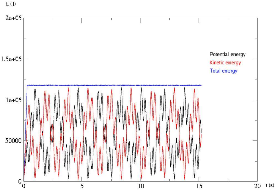
Figure 4: Total, potential and kinetic energies for the simulation of the cylinder over 500000 time-steps

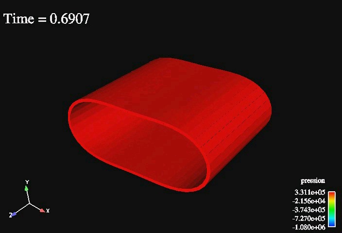
Figure 5: Initial configuration of the cylinder

The preservation of energy is quite satisfactory, even with large displacements in a three-dimensional geometry.

5.3 Static shell test cases

In order to show the versatility of the method, we compare the static deformation obtained with Mka3D (adding damping to the model) to the second and fourth benchmarks for geometric nonlinear shells found in [41].

The first benchmark considered is that of the cantilever subjected to an end moment $\mathcal{M}$. Let $N$ be the number of discrete elements in the length of the beam. We take one element in the two other directions. We immediately see that at the equilibrium, for each particle $I$, the sum of forces is null, and using the boundary conditions, the force $\underline{F}_{IJ}$ between particles is always null. The sum of moments is also zero, and is equal to the end moment $\mathcal{M}$. As $\underline{F}_{IJ}=\underline{0}$, if we denote $\theta_{N}$ the angle between two consecutive particles, using (51),

$$\underline{M}_{IJ}=\underline{M}_{IJ}^{f}=\frac{EI}{2D_{IJ}^{0}}\sin\theta_{N}$$ (46)

If we take the maximum end moment $\mathcal{M}_{max}=2\pi\frac{EI}{L}$, which is the theoretical moment applied to bend the beam into a circle, we obtain :

$$N\theta_{N}=N\arcsin\left(\frac{2\pi}{N}\right)$$ (47)

As $N$ tends to infinity, the deflection angle of the end $N\theta_{N}$ tends to $2\pi$ with second order precision, which indicates a second order convergence to the theoretical solution. This convergence has been checked in practice.

The second benchmark considered is a hemispherical shell with an $18^{\circ}$ circular cutout at its pole, loaded by alternating radial point forces $\mathcal{F}$ at $90^{\circ}$ intervals. The shell is discretized by 16 elements in latitude, 64 elements in longitude and one element in thickness. The initial and deformed geometries are shown on figure 6. The radial deflections at the points of loading A and B are compared with the results obtained in [41] in figure 7. Our results are in very good agreement with the benchmark.

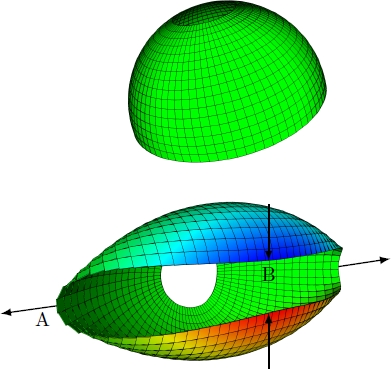
Figure 6: Initial geometry and deformed geometry at $\mathcal{F}=400N$ for the hemispherical shell subjected to alternating radial forces

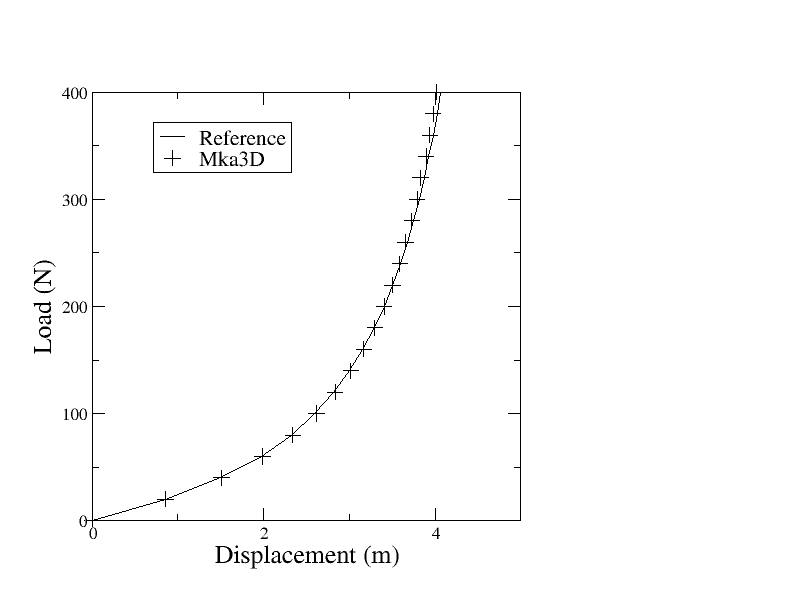
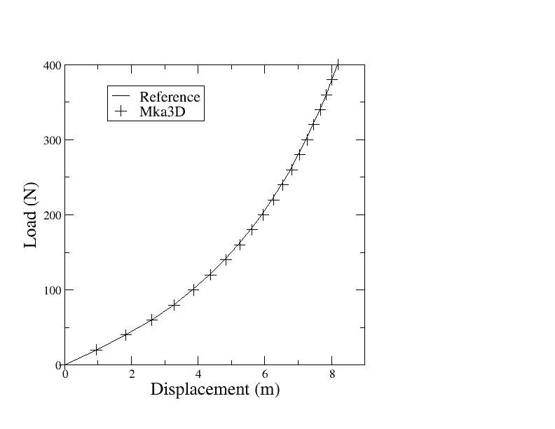
Figure 7: Load-deflection curves for the hemisphere shell at the loading points A (left) and B (right)

6 Conclusion

In this paper, we proposed a numerical discretization of material continuum, allowing for the simulation of three-dimensional wave propagation as well as shell or multibody dynamics, in a monolithic way. It is consistent with the equations of elastodynamics at order 2 in space and in time, and we numerically recover the propagation of seismic waves in the body of the material and at the free surface. Furthermore, the dynamics of the system are written in the form of a Hamiltonian dynamics. Using symplectic schemes, we correctly reproduce the preservation of the system energy. This ensures numerical $L^{2}$-stability of the scheme, and allows long-time stable simulations with large displacements and large deformations. As the method is entirely local and requires no matrix inversion, it can be easily parallelized with domain decomposition. The main restriction is the size of the time-step due to the explicit nature of the integration scheme. This could be remedied by using asynchronous symplectic integrators in order to have local time refinement at small elements and a global larger time-step [31]. This work can be seen as a first step towards using more complex constitutive laws (while still maintaining stability of the scheme), and towards coupling particle dynamics simulation with a fluid dynamics simulation for fluid-structure interaction.

The first author acknowledges the support of CEA under Grant n^∘1045.

We would like to thank Serge Piperno, Tony Lelièvre, Frédéric Legoll and Eric Cancès (Cermics and UR Navier, Ecole des Ponts) for useful discussions and advice on the mathematical and computational aspects of this paper. We also thank Karam Sab (UR Navier, Ecole des Ponts) for pointing us the similarity of our model with Cosserat models. Thanks are also due to Gilles Vilmart for discussions on the resolution of the quaternion scheme.

Appendix A Expression of the equivalent volumetric deformation with a free surface

We need to account for the boundary condition $\underline{\underline{\sigma}}\cdot\underline{n}=\underline{0}$ at every free surface of the particles. We have seen in section 2.3 that the discrete equivalent for $\underline{\underline{\sigma}}\cdot\underline{n}$ is $\underline{F}_{IJ}$. For a given particle $I$, we assume that the particle is surrounded by real particles $J\in\mathcal{V}_{I}$, and by ‘ghost’ particles $J\in\mathcal{V}_{I}^{l}$ at every free boundary. The position of these particles is ajusted in order to satisfy the boundary condition.

The equivalent deformation of particle $I$ can be expressed as in the bulk of the material :

$$\varepsilon_{I}^{v}=\sum_{J\in\mathcal{V}_{I}}{\frac{1}{2}\frac{S_{IJ}}{V_{I}}\underline{\Delta u}_{IJ}\cdot\underline{n}_{IJ}}+\sum_{J\in\mathcal{V}_{I}^{l}}{\frac{1}{2}\frac{S_{IJ}}{V_{I}}\underline{\Delta u}_{IJ}\cdot\underline{n}_{IJ}}$$

For a ghost particle $J\in\mathcal{V}_{I}^{l}$, the boundary condition $\underline{F}_{IJ}\cdot\underline{n}_{IJ}=0$ boils down to :

$$\frac{S_{IJ}}{D_{IJ}^{0}}\frac{E}{1+\nu}\underline{\Delta u}_{IJ}\cdot\underline{n}_{IJ}+S_{IJ}\frac{E\nu}{(1+\nu)(1-2\nu)}\varepsilon_{I}^{v}=0$$ (48)

Summing (48) over the ghost particles, and using the fact that the free volume $V_{I}^{l}$ satisfies

$$V_{I}^{l}=\sum_{J\in\mathcal{V}_{I}^{l}}{\frac{S_{IJ}D_{IJ}^{0}}{6}}$$

we find that the deformation of the links with the ghost particles should follow the equation :

$$\sum_{J\in\mathcal{V}_{I}^{l}}{\frac{1}{2}\frac{S_{IJ}}{V_{I}}\underline{\Delta u}_{IJ}\cdot\underline{n}_{IJ}}=-\frac{3\nu}{1-2\nu}\frac{V_{I}^{l}}{V_{I}+\frac{3\nu}{1-2\nu}V_{I}^{l}}\sum_{J\in\mathcal{V}_{I}}{\frac{1}{2}\frac{S_{IJ}}{V_{I}}\underline{\Delta u}_{IJ}\cdot\underline{n}_{IJ}}$$

Inserting this relation in the expression of $\varepsilon_{I}^{v}$, we check that :

$$\varepsilon_{I}^{v}=\sum_{J\in\mathcal{V}_{I}}{\frac{1}{2}\frac{S_{IJ}}{V_{I}+\frac{3\nu}{1-2\nu}V_{I}^{l}}\underline{\Delta u}_{IJ}\cdot\underline{n}_{IJ}}$$

Appendix B Expression of the coefficients for the flexion and torsion of the particle links

We denote :

$$I_{IJ}^{s} =\iint_{\mathcal{S}_{IJ}}{(\underline{XP_{IJ}}\cdot\underline{s}_{IJ})^{2}dX}$$ (49)

$$I_{IJ}^{t} =\iint_{\mathcal{S}_{IJ}}{(\underline{XP_{IJ}}\cdot\underline{t}_{IJ})^{2}dX}$$ (50)

the principal moments of the interface between particles $I$ and $J$, we require that :

$$\left\{\begin{array}[]{l}\displaystyle\alpha_{n}+\alpha_{s}=\frac{EI_{IJ}^{s}}{S_{IJ}}\\ \displaystyle\alpha_{n}+\alpha_{t}=\frac{EI_{IJ}^{t}}{S_{IJ}}\\ \displaystyle\alpha_{s}+\alpha_{t}=\frac{E(I_{IJ}^{s}+I_{IJ}^{t})}{2(1+\nu)S_{IJ}}\end{array}\right.$$ (51)

The expression of the $\alpha$ is given by :

$$\alpha_{n} =\frac{(1+2\nu)E}{4(1+\nu)S_{IJ}}(I_{IJ}^{s}+I_{IJ}^{t})$$ (52)

$$\alpha_{s} =\frac{E}{4(1+\nu)S_{IJ}}((3+2\nu)I_{IJ}^{s}-(1+2\nu)I_{IJ}^{t})$$ (53)

$$\alpha_{t} =\frac{E}{4(1+\nu)S_{IJ}}((3+2\nu)I_{IJ}^{t}-(1+2\nu)I_{IJ}^{s})$$ (54)

Appendix C Derivation of the forces and torques from the potential energies

The derivation of potential energies is straightforward :

$$\frac{\partial U_{t}}{\partial\underline{X}_{I}} =-\sum_{J\in\mathcal{V}_{I}}{\frac{S_{IJ}}{D_{IJ}^{0}}\frac{E}{1+\nu}\underline{\Delta u}_{IJ}}$$

$$\frac{\partial U_{d}}{\partial\underline{X}_{I}} =-\sum_{J\in\mathcal{V}_{I}}{\frac{E\nu}{(1+\nu)(1-2\nu)}S_{IJ}\varepsilon_{IJ}^{v}\left(\underline{n}_{IJ}+\frac{1}{D_{IJ}}\underline{\Delta u}_{IJ}-\frac{1}{D_{IJ}}(\underline{\Delta u}_{IJ}\cdot\underline{n}_{IJ})\underline{n}_{IJ}\right)}$$

$$\frac{\partial U_{t}}{\partial\underline{\underline{Q}}_{I}} =-\sum_{J\in\mathcal{V}_{I}}{\frac{S_{IJ}}{D_{IJ}^{0}}\frac{E}{1+\nu}\underline{\Delta u}_{IJ}\otimes\underline{X_{I}^{0}P_{IJ}}}$$

$$\frac{\partial U_{d}}{\partial\underline{\underline{Q}}_{I}} =-\sum_{J\in\mathcal{V}_{I}}{\frac{E\nu}{(1+\nu)(1-2\nu)}S_{IJ}\varepsilon_{IJ}^{v}\underline{n}_{IJ}\otimes\underline{X_{I}^{0}P_{IJ}}}$$

$$\frac{\partial U_{f}}{\partial\underline{\underline{Q}}_{I}} =-\sum_{J\in\mathcal{V}_{I}}{S_{IJ}\frac{E}{D_{IJ}^{0}}\left(\alpha_{n}(\underline{\underline{Q}}_{J}\cdot\underline{n}_{IJ}^{0})\otimes\underline{n}_{IJ}^{0}+\alpha_{s}(\underline{\underline{Q}}_{J}\cdot\underline{s}_{IJ})\otimes\underline{s}_{IJ}+\alpha_{t}(\underline{\underline{Q}}_{J}\cdot\underline{t}_{IJ})\otimes\underline{t}_{IJ}\right)}$$

Using the expression of the force $\underline{F}_{IJ}$ between particles $I$ and $J$ :

$$\underline{F}_{IJ}=\frac{S_{IJ}}{D_{IJ}^{0}}\frac{E}{1+\nu}\underline{\Delta u}_{IJ}+S_{IJ}\frac{E\nu}{(1+\nu)(1-2\nu)}\varepsilon_{IJ}^{v}\left(\underline{n}_{IJ}+\frac{1}{D_{IJ}}\underline{\Delta u}_{IJ}-\frac{1}{D_{IJ}}(\underline{\Delta u}_{IJ}\cdot\underline{n}_{IJ})\underline{n}_{IJ}\right)$$

we obtain :

$$m_{I}\underline{\dot{v}}_{I}=\underline{\dot{T}}_{I}=\underline{F}_{IJ}$$

For the rotational part, it is easily obtained that :

$$\underline{\underline{j}}(\underline{\underline{R}}_{I}\underline{\Omega}_{I})=\underline{\underline{j}}(\underline{\Omega}_{I})\underline{\underline{D}}-\underline{\underline{D}}\underline{\underline{j}}(\underline{\Omega}_{I})=\underline{\underline{P}}_{I}\cdot{\underline{\underline{Q}}}^{\text{T}}-\underline{\underline{Q}}_{I}\cdot{\underline{\underline{P}}}^{\text{T}}$$

Deriving in time, we obtain :

$$\frac{d}{dt}\left(\underline{\underline{j}}(\underline{\underline{R}}_{I}\cdot\underline{\Omega}_{I})\right)=-\left(\frac{\partial H_{h}}{\partial\underline{\underline{Q}}_{I}}\right){\underline{\underline{Q}}_{I}}^{\text{T}}+\underline{\underline{Q}}_{I}{\left(\frac{\partial H_{h}}{\partial\underline{\underline{Q}}_{I}}\right)}^{\text{T}}$$

Using the fact that :

$$(\underline{a}\otimes\underline{b})\cdot\underline{\underline{Q}}=\underline{a}\otimes({\underline{\underline{Q}}}^{\text{T}}\cdot\underline{b})$$

we get :

$$\frac{\partial U_{t}}{\partial\underline{\underline{Q}}_{I}}\cdot{\underline{\underline{Q}}_{I}}^{\text{T}}=-\sum_{J\in\mathcal{V}_{I}}{\frac{S_{IJ}}{D_{IJ}^{0}}\frac{E}{1+\nu}\underline{\Delta u}_{IJ}\otimes(\underline{\underline{Q}}_{I}\cdot\underline{X_{I}^{0}P_{IJ}})}$$ (55)

$$\frac{\partial U_{d}}{\partial\underline{\underline{Q}}_{I}}\cdot{\underline{\underline{Q}}_{I}}^{\text{T}}=-\sum_{J\in\mathcal{V}_{I}}{\frac{E\nu}{(1+\nu)(1-2\nu)}S_{IJ}\varepsilon_{IJ}^{v}\underline{n}_{IJ}\otimes(\underline{\underline{Q}}_{I}\cdot\underline{X_{I}^{0}P_{IJ}})}$$ (56)

$$\frac{\partial U_{f}}{\partial\underline{\underline{Q}}_{I}}\cdot{\underline{\underline{Q}}_{I}}^{\text{T}}=-\sum_{J\in\mathcal{V}_{I}}{S_{IJ}\frac{E}{D_{IJ}^{0}}\left(\alpha_{n}(\underline{\underline{Q}}_{J}\cdot\underline{n}_{IJ}^{0})\otimes(\underline{\underline{Q}}_{I}\cdot\underline{n}_{IJ}^{0})+\alpha_{s}(\underline{\underline{Q}}_{J}\cdot\underline{s}_{IJ})\otimes(\underline{\underline{Q}}_{I}\cdot\underline{s}_{IJ})\right.}\\ {\left.+\alpha_{t}(\underline{\underline{Q}}_{J}\cdot\underline{t}_{IJ})\otimes(\underline{\underline{Q}}_{I}\cdot\underline{t}_{IJ})\right)}$$ (57)

Denoting $\text{symm}()$ and $\text{skew}()$ the symmetric and skew-symmetric parts of a matrix, we note that for any $\underline{a}$ and $\underline{b}$ :

$$\underline{\underline{j}}(\underline{a}\wedge\underline{b})=-\text{skew}(\underline{a}\otimes\underline{b})$$

Using the expression of the torques $\underline{M}_{IJ}^{t}$ and $\underline{M}_{IJ}^{f}$ :

$$\underline{M}_{IJ}^{t}=\frac{S_{IJ}}{D_{IJ}^{0}}\frac{E}{1+\nu}(\underline{\underline{Q}}_{I}\cdot\underline{X_{I}^{0}P_{IJ}})\wedge\underline{\Delta u}_{IJ}+\frac{E\nu}{(1+\nu)(1-2\nu)}\varepsilon_{IJ}^{v}S_{IJ}(\underline{\underline{Q}}_{I}\cdot\underline{X_{I}^{0}P_{IJ}})\wedge\underline{n}_{IJ}$$

$$\underline{M}_{IJ}^{f}=\frac{S_{IJ}}{D_{IJ}^{0}}\left(\alpha_{n}(\underline{\underline{Q}}_{I}\cdot\underline{n}_{IJ}^{0})\wedge(\underline{\underline{Q}}_{J}\cdot\underline{n}_{IJ}^{0})\right.\left.+\alpha_{s}(\underline{\underline{Q}}_{I}\cdot\underline{s}_{IJ})\wedge(\underline{\underline{Q}}_{J}\cdot\underline{s}_{IJ})\right.\left.+\alpha_{t}(\underline{\underline{Q}}_{I}\cdot\underline{t}_{IJ})\wedge(\underline{\underline{Q}}_{J}\cdot\underline{t}_{IJ})\right)$$

equation (15) gives us the equation on the angular velocity :

$$\frac{d}{dt}\left(\underline{\underline{R}}_{I}\cdot\underline{\Omega}_{I}\right)=\sum_{J\in\mathcal{V}_{I}}{\underline{M}_{IJ}^{t}+\underline{M}_{IJ}^{f}}$$

Appendix D Details on the implementation of the RATTLE scheme with forces and torques

For forces, the relation is simple :

$$\frac{\partial U_{h}}{\partial\underline{X}_{I}}(\underline{X},\underline{\underline{Q}})=-\sum_{J\in\mathcal{V}_{I}}{\underline{F}_{IJ}}$$

For torques, we have :

$$\frac{\partial U_{h}}{\partial\underline{\underline{Q}}_{I}}(\underline{X},\underline{\underline{Q}})=\dot{\underline{\underline{P}}}_{I}-\underline{\underline{Q}}_{I}\underline{\underline{\Lambda}}_{I}$$

where $\underline{\underline{\Lambda}}_{I}$ is the symmetric matrix of Lagrange multipliers associated with constraint $\underline{\underline{Q}}_{I}\cdot{\underline{\underline{Q}}_{I}}^{\text{T}}=\underline{\underline{Id}}$. On the other hand,

$$\underline{\underline{j}}\left(\sum_{J\in\mathcal{V}_{I}}{\underline{M}_{IJ}}\right)= \underline{\underline{\dot{P}}}_{I}\cdot{\underline{\underline{Q}}_{I}}^{\text{T}}+\underline{\underline{P}}_{I}\cdot{\underline{\underline{\dot{Q}}}_{I}}^{\text{T}}-\underline{\underline{\dot{Q}}}_{I}\cdot{\underline{\underline{P}}_{I}}^{\text{T}}-\underline{\underline{Q}}_{I}\cdot{\underline{\underline{\dot{P}}}_{I}}^{\text{T}}$$

$$= \underline{\underline{Q}}_{I}\cdot{\left(\frac{\partial U_{h}}{\partial\underline{\underline{Q}}_{I}}(\underline{X},\underline{\underline{Q}})\right)}^{\text{T}}-\frac{\partial U_{h}}{\partial\underline{\underline{Q}}_{I}}(\underline{X},\underline{\underline{Q}})\cdot{\underline{\underline{Q}}_{I}}^{\text{T}}$$

as the $\underline{\underline{\Lambda}}_{I}$ are symmetric. Therefore, there exists a symmetric matrix $\underline{\underline{\Lambda}}^{0}_{I}$ such that :

$$\frac{\partial U_{h}}{\partial\underline{\underline{Q}}_{I}}(\underline{X},\underline{\underline{Q}})=\left(-\frac{1}{2}\underline{\underline{j}}\left(\sum_{J\in\mathcal{V}_{I}}{\underline{M}_{IJ}}\right)-\underline{\underline{\Lambda}}^{0}_{I}\right)\cdot\underline{\underline{Q}}_{I}$$

We denote :

$$\underline{\mathcal{F}}_{I}^{n} =\sum_{J\in\mathcal{V}_{I}}{\underline{F}_{IJ}}$$

$$\underline{\mathcal{M}}_{I}^{n} =\sum_{J\in\mathcal{V}_{I}}{\underline{M}_{IJ}}$$

where forces $\underline{F}_{IJ}$ and torques $\underline{M}_{IJ}$ have been computed with positions $\underline{X}^{n}$ and $\underline{\underline{Q}}^{n}$.

We can rewrite equations (29) to (35) as follows :

$$\underline{T}_{I}^{n+1/2} =\underline{P}_{I}^{n}+\frac{\Delta t}{2}\underline{\mathcal{F}}_{I}^{n}$$ (58)

$$\underline{\underline{P}}_{I}^{n+1/2} =\underline{\underline{P}}_{I}^{n}+\frac{\Delta t}{4}\underline{\underline{j}}(\underline{\mathcal{M}}_{I}^{n})\underline{\underline{Q}}_{I}^{n}+\frac{\Delta t}{2}(\underline{\underline{\Lambda}}_{I}^{n}+\underline{\underline{\Lambda}}_{I}^{n,0})\underline{\underline{Q}}_{I}^{n}$$ (59)

$$\underline{X}_{I}^{n+1} =\underline{X}_{I}^{n}+\frac{\Delta t}{m_{I}}\underline{T}_{I}^{n+1/2}$$ (60)

$$\underline{\underline{Q}}_{I}^{n+1} =\underline{\underline{Q}}_{I}^{n}+\Delta t\underline{\underline{P}}_{I}^{n+1/2}\underline{\underline{D}}_{I}^{-1}$$ (61)

$$\text{where }\underline{\underline{\Lambda}}_{I}^{n}\text{ is such that }{\underline{\underline{Q}}_{I}^{n+1}}^{\text{T}}\cdot\underline{\underline{Q}}_{I}^{n+1}=\underline{\underline{Id}}$$ (62)

$$\underline{T}_{I}^{n+1} =\underline{T}_{I}^{n+1/2}+\frac{\Delta t}{2}\underline{\mathcal{F}}_{I}^{n+1}$$ (63)

$$\underline{\underline{P}}_{I}^{n+1} =\underline{\underline{P}}_{I}^{n+1/2}+\frac{\Delta t}{4}\underline{\underline{j}}(\underline{\mathcal{M}}_{I}^{n+1})\underline{\underline{Q}}_{I}^{n+1}+\frac{\Delta t}{2}(\underline{\underline{\tilde{\Lambda}}}_{I}^{n+1}+\underline{\underline{\tilde{\Lambda}}}_{I}^{n+1,0})\underline{\underline{Q}}_{I}^{n+1},$$ (64)

$$\text{where }\underline{\underline{\Lambda}}_{I}^{n}\text{ is such that }{\underline{\underline{Q}}_{I}^{n+1}}^{\text{T}}\cdot\underline{\underline{P}}_{I}^{n+1}\cdot\underline{\underline{D}}_{I}^{-1}+\underline{\underline{D}}_{I}^{-1}\cdot{\underline{\underline{P}}_{I}^{n+1}}^{\text{T}}\cdot\underline{\underline{Q}}_{I}^{n+1}=\underline{\underline{0}}$$ (65)

Appendix E Resolution of the nonlinear step of the RATTLE time-scheme

In this appendix, we examine the resolution of the nonlinear step of the RATTLE time-scheme described in section 4.3. We determine conditions on the time-step $\Delta t$ that ensure convergence of the iterative algorithm (40)–(43) in a certain neighbourhood of identity, and we conclude on the existence and uniqueness of a solution in this neighbourhood.

We denote $\mathcal{B}(\underline{0},r)$ the ball of center $\underline{0}$ and radius $r$ :

$$\mathcal{B}(\underline{0},r)=\left\{(e_{1},e_{2},e_{3})/e_{1}^{2}+e_{2}^{2}+e_{3}^{2}<r^{2}\right\}$$

Using the numerical scheme described in section 4.3, we first show that it stabilizes a ball included in $\mathcal{B}(\underline{0},\frac{\sqrt{2}}{2})$, under a CFL-type condition on $\Delta t$. We then show convergence in that same ball, and we conclude on convergence to the unique fixed point.

E.1 The iterative scheme is bounded

Starting with a given $(e_{0},e_{1},e_{2},e_{3})$ computed in the previous iteration, such that $e_{0}^{2}+e_{1}^{2}+e_{2}^{2}+e_{3}^{2}=1$, the iterative scheme (40)–(43) gives the new quadruplet $(e_{0}^{*},e_{1}^{*},e_{2}^{*},e_{3}^{*})$ defined by :

$$e_{1}^{*} =\frac{\Delta t\alpha_{1}-2(d_{2}-d_{3})e_{2}e_{3}}{2(d_{2}+d_{3})e_{0}}$$

$$e_{2}^{*} =\frac{\Delta t\alpha_{2}-2(d_{3}-d_{1})e_{1}e_{3}}{2(d_{1}+d_{3})e_{0}}$$

$$e_{3}^{*} =\frac{\Delta t\alpha_{3}-2(d_{1}-d_{2})e_{1}e_{2}}{2(d_{1}+d_{2})e_{0}}$$

$$e_{0}^{*} =\sqrt{1-(e_{1}^{*})^{2}-(e_{2}^{*})^{2}-(e_{3}^{*})^{2}}$$

For this scheme to be well-defined, $(e_{1}^{*},e_{2}^{*},e_{3}^{*})$ should be in $\mathcal{B}(\underline{0},1)$. We impose a stronger condition, with $(e_{1},e_{2},e_{3})$ and $(e_{1}^{*},e_{2}^{*},e_{3}^{*})$ in $\mathcal{B}(\underline{0},\beta)$ where $\beta$ is less than $\frac{1}{2}$.

Suppose that :

$$e_{1}^{2}+e_{2}^{2}+e_{3}^{2}<\beta$$

We want to have :

$$(e_{1}^{*})^{2}+(e_{2}^{*})^{2}+(e_{3}^{*})^{2}<\beta$$

As $e_{0}^{2}+e_{1}^{2}+e_{2}^{2}+e_{3}^{2}=1$, we also have $e_{0}^{2}>1-\beta$. Since :

$$|e_{2}e_{3}|\leq\frac{1}{2}(e_{2}^{2}+e_{3}^{2})<\frac{\beta}{2}$$

we obtain :

$$|e_{1}^{*}|<\frac{1}{2\sqrt{1-\beta}(d_{2}+d_{3})}(|\Delta t\alpha_{1}|+\beta|d_{2}-d_{3}|)$$

Let us define $I_{1}=d_{2}+d_{3}$, $I_{2}=d_{1}+d_{3}$, $I_{3}=d_{1}+d_{2}$ and :

$$f(\beta)=\frac{1}{4(1-\beta)}\left[\Delta t^{2}\left(\frac{|\alpha_{1}|^{2}}{I_{1}^{2}}+\frac{|\alpha_{2}|^{2}}{I_{2}^{2}}+\frac{|\alpha_{3}|^{2}}{I_{3}^{2}}\right)\right.\left.+2\beta\Delta t\left(\frac{|d_{2}-d_{3}||\alpha_{1}|}{I_{1}^{2}}+\frac{|d_{3}-d_{1}||\alpha_{2}|}{I_{2}^{2}}\right.\right.\left.\left.+\frac{|d_{1}-d_{2}||\alpha_{3}|}{I_{3}^{2}}\right)\right.\\ \left.+\beta^{2}\left(\frac{|d_{2}-d_{3}|^{2}}{I_{1}^{2}}+\frac{|d_{3}-d_{1}|^{2}}{I_{2}^{2}}+\frac{|d_{1}-d_{2}|^{2}}{I_{3}^{2}}\right)\right]$$

then the previous assumptions imply that :

$$(e_{1}^{*})^{2}+(e_{2}^{*})^{2}+(e_{3}^{*})^{2}<f(\beta)$$

Therefore, a sufficient condition for the scheme to be bounded is $f(\beta)\leq\beta$. We know that :

$$\frac{|d_{2}-d_{3}|}{I_{1}}=\frac{|d_{2}-d_{3}|}{d_{2}+d_{3}}\leq 1$$

as the $d_{i}$ are positive. Then :

$$f(\beta)\leq\frac{1}{4(1-\beta)}\left(\Delta t^{2}\left[\frac{|\alpha_{1}|^{2}}{I_{1}^{2}}+\frac{|\alpha_{2}|^{2}}{I_{2}^{2}}+\frac{|\alpha_{3}|^{2}}{I_{3}^{2}}\right)\right.\left.+2\beta\Delta t\left(\frac{|\alpha_{1}|}{I_{1}}+\frac{|\alpha_{2}|}{I_{2}}+\frac{|\alpha_{3}|}{I_{3}}\right)+3\beta^{2}\right]$$

Hence, a sufficient condition for $f(\beta)\leq\beta$ to hold is :

$$\Delta t^{2}\left(\frac{|\alpha_{1}|^{2}}{I_{1}^{2}}+\frac{|\alpha_{2}|^{2}}{I_{2}^{2}}+\frac{|\alpha_{3}|^{2}}{I_{3}^{2}}\right)+2\beta\Delta t\left(\frac{|\alpha_{1}|}{I_{1}}+\frac{|\alpha_{2}|}{I_{2}}+\frac{|\alpha_{3}|}{I_{3}}\right)+7\beta^{2}-4\beta<0$$ (66)

Let us define :

$$B =\frac{|\alpha_{1}|}{I_{1}}+\frac{|\alpha_{2}|}{I_{2}}+\frac{|\alpha_{3}|}{I_{3}}$$

$$C =\frac{|\alpha_{1}|^{2}}{I_{1}^{2}}+\frac{|\alpha_{2}|^{2}}{I_{2}^{2}}+\frac{|\alpha_{3}|^{2}}{I_{3}^{2}}$$

A sufficient condition to obtain (66) is to have $\Delta t\leq\tilde{\Delta t}$ with :

$$\tilde{\Delta t}=\frac{-2\beta B+\sqrt{4\beta^{2}B^{2}-4(7\beta^{2}-4\beta)C}}{2C}$$

As we supposed that $0<\beta<\frac{1}{2}<\frac{4}{7}$, $7\beta^{2}-4\beta<0$. We also know that $B^{2}\leq 3C$ and $C\leq B^{2}$, and it follows that :

$$\tilde{h}\geq\frac{2\sqrt{\frac{\beta-\beta^{2}}{3}}-\beta}{B}$$

In the end, we have the following lemma :

Lemma E.1

Let us choose $0<\beta<\frac{1}{2}$ and $\Delta t>0$ such that :

$$\Delta t\left(\frac{|\alpha_{1}|}{I_{1}}+\frac{|\alpha_{2}|}{I_{2}}+\frac{|\alpha_{3}|}{I_{3}}\right)\leq 2\sqrt{\frac{\beta-\beta^{2}}{3}}-\beta$$ (67)

If $(e_{1},e_{2},e_{3})\in\mathcal{B}(0,\sqrt{\beta})$, then $(e_{1}^{*},e_{2}^{*},e_{3}^{*})\in\mathcal{B}(\underline{0},\sqrt{\beta})$.

E.2 The iterative scheme is a contraction

Following the previous subsection, suppose that $(e_{1},e_{2},e_{3})$ and $(f_{1},f_{2},f_{3})$ are in $\mathcal{B}(0,\sqrt{\beta})$, and let $e_{0}=\sqrt{1-e_{1}^{2}-e_{2}^{2}-e_{3}^{2}}$ and $f_{0}=\sqrt{1-f_{1}^{2}-f_{2}^{2}-f_{3}^{2}}$. We define $e^{*}$ and $f^{*}$ as before. We show here that $\lVert e^{*}-f^{*}\rVert\leq\rho\lVert e-f\rVert$, with $0<\rho<1$.

We compute :

$$e_{1}^{*}-f_{1}^{*}=\frac{(d_{2}-d_{3})}{I_{1}e_{0}}\left[(f_{2}-e_{2})\left(\frac{f_{3}+e_{3}}{2}\right)\right.\left.+(f_{3}-e_{3})\left(\frac{f_{2}+e_{2}}{2}\right)\right]+\frac{f_{0}-e_{0}}{e_{0}}f_{1}^{*}$$

We then use the fact that $\frac{|d_{2}-d_{3}|}{I_{1}}<1$. As the same type of results hold with a circular permutation of indices $x$, $y$ and $z$, we let $\lVert\cdot\rVert$ the euclidian norm in $\mathbb{R}^{3}$ on $(e_{1},e_{2},e_{3})$, and we find :

$$\lVert e^{*}-f^{*}\rVert^{2}\leq 2\frac{\left(\frac{f_{2}+e_{2}}{2}\right)^{2}+\left(\frac{f_{3}+e_{3}}{2}\right)^{2}}{e_{0}^{2}}(f_{1}-e_{1})^{2}+2\frac{\left(\frac{f_{1}+e_{1}}{2}\right)^{2}+\left(\frac{f_{3}+e_{3}}{2}\right)^{2}}{e_{0}^{2}}(f_{2}-e_{2})^{2}\\ +2\frac{\left(\frac{f_{1}+e_{1}}{2}\right)^{2}+\left(\frac{f_{2}+e_{2}}{2}\right)^{2}}{e_{0}^{2}}(f_{3}-e_{3})^{2}+\frac{4}{e_{0}^{2}}(f_{2}-e_{2})(f_{3}-e_{3})\left(\frac{f_{2}+e_{2}}{2}\right)\left(\frac{f_{3}+e_{3}}{2}\right)\\ +\frac{4}{e_{0}^{2}}(f_{1}-e_{1})(f_{3}-e_{3})\left(\frac{f_{1}+e_{1}}{2}\right)\left(\frac{f_{3}+e_{3}}{2}\right)+\frac{4}{e_{0}^{2}}(f_{1}-e_{1})(f_{2}-e_{2})\left(\frac{f_{1}+e_{1}}{2}\right)\left(\frac{f_{2}+e_{2}}{2}\right)\\ +2\frac{(f_{1}^{*})^{2}+(f_{2}^{*})^{2}+(f_{3}^{*})^{2}}{e_{0}^{2}}(f_{0}-e_{0})^{2}$$

Since :

$$\frac{4}{e_{0}^{2}}(f_{2}-e_{2})(f_{3}-e_{3})\left(\frac{f_{2}+e_{2}}{2}\right)\left(\frac{f_{3}+e_{3}}{2}\right)\leq\frac{2}{e_{0}^{2}}\left[(f_{2}-e_{2})^{2}\left(\frac{f_{2}+e_{2}}{2}\right)^{2}\right.\left.+(f_{3}-e_{3})^{2}\left(\frac{f_{3}+e_{3}}{2}\right)^{2}\right]$$

we have :

$$\lVert e^{*}-f^{*}\rVert^{2}\leq\frac{2}{e_{0}^{2}}\left(\lVert\frac{e+f}{2}\rVert^{2}\lVert e-f\rVert^{2}+\lVert f^{*}\rVert^{2}(f_{0}-e_{0})^{2}\right)$$

We also have :

$$(f_{0}-e_{0})^{2}\leq\frac{\lVert\frac{e+f}{2}\rVert^{2}}{(\frac{e_{0}+f_{0}}{2})^{2}}\lVert e-f\rVert^{2}$$

In the end, we obtain the upper bound :

$$\lVert e^{*}-f^{*}\rVert^{2}\leq 2\frac{\lVert\frac{e+f}{2}\rVert^{2}}{e_{0}^{2}}\left(1+\frac{\lVert f^{*}\rVert^{2}}{\left(\frac{e_{0}+f_{0}}{2}\right)^{2}}\right)\lVert e-f\rVert^{2}$$

If we take the same hypotheses as in the first subsection, that is, $(e_{1},e_{2},e_{3})\in\mathcal{B}(\underline{0},\sqrt{\beta})$ and $(f_{1},f_{2},f_{3})\in\mathcal{B}(\underline{0},\sqrt{\beta})$, and $h$ such that $(e_{1}^{*},e_{2}^{*},e_{3}^{*})\in\mathcal{B}(\underline{0},\sqrt{\beta})$ and $(f_{1}^{*},f_{2}^{*},f_{3}^{*})\in\mathcal{B}(\underline{0},\sqrt{\beta})$, then due to the convexity of $\mathcal{B}(\underline{0},\sqrt{\beta})$, we have :

$$\lVert\frac{e+f}{2}\rVert^{2}<\beta$$

and moreover, as $e_{0}^{2}>1-\beta$ et $f_{0}^{2}>1-\beta$, then $\left(\frac{e_{0}+f_{0}}{2}\right)^{2}>1-\beta$.

Then :

$$2\frac{\lVert\frac{e+f}{2}\rVert^{2}}{e_{0}^{2}}\left(1+\frac{\lVert f^{*}\rVert^{2}}{\left(\frac{e_{0}+f_{0}}{2}\right)^{2}}\right)\leq 2\frac{\beta}{1-\beta}\left(1+\frac{\beta}{1-\beta}\right)=\frac{2\beta}{(1-\beta)^{2}}$$

In order to have a scheme which is a contraction, it is sufficient to impose :

$$\frac{2\beta}{(1-\beta)^{2}}\leq 1$$

As $0<\beta<\frac{1}{2}$, it is sufficient to choose :

$$\beta\leq 2-\sqrt{3}$$

E.3 Optimization on constant $\beta$

Optimizing the stability condition (67) on $\Delta t$, we obtain the following optimal value of $\beta$ :

$$\beta_{\text{max}}=\frac{7-\sqrt{21}}{14}\approx 0.17$$

E.4 Conclusion

If we take the time-step $\Delta t$ such that :

$$\Delta t\left(\frac{|\alpha_{1}|}{I_{1}}+\frac{|\alpha_{2}|}{I_{2}}+\frac{|\alpha_{3}|}{I_{3}}\right)\leq 2\sqrt{\frac{\beta_{max}-\beta_{max}^{2}}{3}}-\beta_{max}\approx 0.26$$

then the iterative scheme starting with $(1,0,0,0)$ converges to the unique solution of the nonlinear problem in $\mathcal{B}(\underline{0},\sqrt{\frac{7-\sqrt{21}}{14}})$, and the convergence speed is geometric with a rate $\rho<1$. In addition, $\rho<28-6\sqrt{21}\approx 0.5$. We thus have proved existence and uniqueness of the solution in $\mathcal{B}(\underline{0},\frac{\sqrt{2}}{2})$.

References

- [1] Andersen HC. RATTLE: A ”velocity” version of the SHAKE algorithm for molecular dynamics calculations. Journal of Computational Physics 1983; 52(1):24–34.
- [2] Antoci C, Gallati M, Sibilla S. Numerical simulation of fluid-structure interaction by SPH. Computers & Structures 2007; 85(11–14, Sp. Iss. SI):879–890, 4th MIT Conference on Computational Fluid and Solid Mechanics, Cambridge, MA, JUN 13-15, 2007.
- [3] Bonet J, Lok TSL. Variational and momentum preservation aspects of Smooth Particle Hydrodynamic formulations. Computer Methods in Applied Mechanics and Engineering 1999; 180(1–2):97–115.
- [4] Cundall PA, Strack ODL. A discrete numerical model for granular assemblies. Geotechnique 1979; 29(1):47–65.
- [5] D’Addetta GA, Kun F, Ramm E. On the application of a discrete model to the fracture process of cohesive granular materials. Granular Matter 2002; 4:77–90.
- [6] De Hoop AT. A modification of Cagniard’s method for solving seismic pulse problem. Applied Scientific Research 1960; B8:349–356.
- [7] Eringen AC. Theory of micropolar elasticity. In Fracture, Liebowitz H (ed); Academic Press: New York, 1968; 2:621–729.
- [8] Fahrenthold EP, Horban BA. An improved hybrid particle-element method for hypervelocity impact simulation. International Journal of Impact Engineering 2001; 26:169–178; Symposium on Hypervelocity Impact, Galveston, Texas, Nov 06-10, 2000.
- [9] Fahrenthold EP, Shivarama R. Extension and validation of a hybrid particle-finite element method for hypervelocity impact simulation. International Journal of Impact Engineering 2003; 29(1–10):237–246; Hypervelocity Impact Symposium, Noordwijk, Netherlands, Dec 07-11, 2003.
- [10] Feng YT, Han K, Li CF, Owen DRJ. Discrete thermal element modelling of heat conduction in particle systems: Basic formulations. Journal of Computational Physics 2008; 227(10):5072–5089.
- [11] Forest S, Pradel F, Sab K. Asymptotic analysis of heterogeneous Cosserat media. International Journal of Solids and Structures 2001; 38:4585–4608.
- [12] Gingold RA, Monaghan JJ. Smoothed Particle Hydrodynamics : Theory and Application to Nonspherical Stars. Monthly Notices of the Royal Astronomical Society 1977; 181:375–389.
- [13] Gonzalez O. Exact energy and momentum conserving algorithms for general models in nonlinear elasticity. Computer Methods in Applied Mechanics and Engineering 2000; 190:1763–1783.
- [14] Hairer E, Vilmart G. Preprocessed discrete Moser-Veselov algorithm for the full dynamics of a rigid body. Journal of Physics A: Mathematical and General 2006; 39:13225–13235.
- [15] Hairer E, Lubich C, Wanner G. Geometric Numerical Integration : Structure-Preserving Algorithms for Ordinary Differential Equations (2nd edn). Springer Series in Computational Mathematics, vol. 31. Springer-Verlag, 2006.
- [16] Han K, Feng YT, Owen DRJ. Coupled lattice Boltzmann and discrete element modelling of fluid-particle interaction problems. Computers & Structures 2007; 85(11–14, Sp. Iss. SI):1080–1088; 4th MIT Conference on Computational Fluid and Solid Mechanics, Cambridge, MA, JUN 13-15, 2007.
- [17] Hauret P, Le Tallec P. Energy-controlling time integration methods for nonlinear elastodynamics and low-velocity impact. Computer Methods in Applied Mechanics and Engineering 2006; 195:4890–4916.
- [18] Hicks DL, Swegle JW, Attaway SW. Conservative smoothing stabilizes discrete-numerical instabilities in SPH material dynamics computations. Applied Mathematics and Computation 1997; 85(2–3):209–226.
- [19] Hoover WG. Smooth Particle Applied Mechanics : The State of the Art; Advanced Series in Nonlinear Dynamics, vol. 25. World Scientific, 2006.
- [20] Hoover WG, Arhurst WT, Olness RJ. Two-Dimensional Studies of Crystal Stability and Fluid Viscosity. Journal of Chemical Physics 1974; 60:4043–4047.
- [21] Ibrahimbegovic A, Delaplace A. Microscale and mesoscale discrete models for dynamic fracture of structures built of brittle material. Computers & Structures 2003; 81(12):1255–1265.
- [22] Koo JC, Fahrenthold EP. Discrete Hamilton’s equations for arbitrary Lagrangian-Eulerian dynamics of viscous compressible flow. Computer Methods in Applied Mechanics and Engineering 2000; 189(3):875–900.
- [23] Koshizuka S, Oka Y. Moving-Particle Semi-implicit method for fragmentation of incompressible fluid. Nuclear Science and Engineering 1996; 123:421–434.
- [24] Koshizuka S, Nobe A, Oka Y. Numerical analysis of breaking waves using the Moving Particle Semi-implicit method. International Journal for Numerical Methods in Fluids 1998; 26:751–769.
- [25] Koshizuka S, Song MS, Oka Y. A particle method for three-dimensional elastic analysis. In Proceedings of the 6th World Congress Computational Mechanics (WCCM VI), Beijing 2004.
- [26] Kun F, Herrmann H. A study of fragmentation processes using a discrete element method. Computer Methods in Applied Mechanics and Engineering 1996; 138(1–4):3–18.
- [27] Lamb H. On the propagation of tremors over the surface of an elastic solid. Philosophical Transactions of the Royal Society of London A 1904; 203:1–42.
- [28] Laursen TA, Meng XN. A new solution procedure for application of energy-conserving algorithms to general constitutive models in nonlinear elastodynamics. Computer Methods in Applied Mechanics and Engineering 2001; 190:6309–6322.
- [29] Lee CJK, Noguchi H, Koshizuka S. Fluid-shell structure interaction analysis by coupled particle and finite element method. Computers & Structures 2007; 85(11–14, Sp. Iss. SI):688–697; 4th MIT Conference on Computational Fluid and Solid Mechanics, Cambridge, MA, JUN 13-15, 2007.
- [30] Leimkuhler BJ, Skeel RD. Symplectic numerical integrators in constrained Hamiltonian systems. Journal of Computational Physics 1994; 112(1):117–125.
- [31] Lew A, Marsden JE, Ortiz M, West M. Variational time integrators. International Journal for Numerical Methods in Engineering 2004; 60:153–212.
- [32] Libersky LD, Petschek AG, Carney TC, Hipp JR, Allahdadi FA. High strain Lagrangian hydrodynamics: a three-dimensional SPH code for dynamic material response. Journal of Computational Physics 1993; 109(1):76–83.
- [33] Lucy LB. A numerical approach to the testing of the fission hypothesis. Astronomical Journal 1977; 82:1013–1024.
- [34] Mariotti C. Lamb’s problem with the lattice model Mka3D. Geophysical Journal International 2007; 171:857–864.
- [35] Monaghan JJ. Simulating free surface flows with SPH. Journal of Computational Physics 1994; 110(2):399–406.
- [36] Potyondy DO, Cundall PA. A bonded-particle model for rock. International Journal of Rock Mechanics and Mining Science 2004; 41:1329–1364.
- [37] Ries A, Wolf DE, Unger T. Shear zones in granular media: Three-dimensional contact dynamics simulation. Physical Review E 2007; 76(5)
- [38] Simo JC, Tarnow N, Wong KK. Exact energy-momentum conserving algorithms and symplectic schemes for nonlinear dynamics. Computer Methods in Applied Mechanics and Engineering 1992; 100:63–116.
- [39] Suzuki Y, Koshizuka S. A Hamiltonian particle method for non-linear elastodynamics. International Journal for Numerical Methods in Engineering 2008; 74(8):1344–1373.
- [40] Swegle JW, Hicks DL, Attaway SW. Smoothed Particle Hydrodynamics stability analysis. Journal of Computational Physics 1995; 116(1):123–134.
- [41] Sze KY, Liu XH, Lo SH. Popular benchmark problems for geometric nonlinear analysis of shells. Finite Element in Analysis and Design 2004; 40:1551–1569.
- [42] Yserentant H. A new class of particle methods. Numerische Mathematik 1997; 76(1):87–109.