Finite-temperature local protein sequence alignment:
percolation and free-energy distribution

Abstract

Sequence alignment is a tool in bioinformatics that is used to find homological relationships in large molecular databases. It can be mapped on the physical model of directed polymers in random media. We consider the finite-temperature version of local sequence alignment for proteins and study the transition between the linear phase and the biologically relevant logarithmic phase, where the free-energy grows linearly or logarithmically with the sequence length. By means of numerical simulations and finite-size scaling analysis we determine the phase diagram in the plane that is spanned by the gap costs and the temperature. We use the most frequently used parameter set for protein alignment. The critical exponents that describe the parameter driven transition are found to be explicitly temperature dependent.

Furthermore, we study the shape of the (free-) energy distribution close to the transition by rare-event simulations down to probabilities of the order $10^{-64}$. It is well known that, in the logarithmic region, the optimal score distribution ($T=0$) is described by a modified Gumbel distribution. We confirm that this also applies for the free-energy distribution ($T>0$). However, in the linear phase, the distribution crosses over to a modified Gaussian distribution.

I Introduction

Biological sequence analysis is an interdisciplinary scientific field which uses concepts from statistics, computer science and molecular biology. Some approaches used in the context of sequence analysis are, from a conceptional point of view, related to models in statistical mechanics of disordered systems. One of the most fundamental tools in the area of sequence analysis is sequence alignment (see for example [1, 2]). It is used to quantify similarities between two (or more) biological sequences, like DNA, proteins or RNA. Modern search tools for large databases, like BLAST [3] or FASTA [4], heavily rely on sequence alignment algorithms.

In this article we consider algorithms for pairwise local protein alignment which aims at finding “conserved” regions of two input protein sequences. The most prominent example is the Smith-Waterman algorithm [5]. The algorithm finds optimal alignments (OA) according to an objective function. Each alignment is assigned a score which is maximal for optimal alignments. The optimal alignment score serves as a scalar measure of similarity of the input sequences. Since alignments have a geometrical interpretation as directed paths [6], the problem of finding an optimal alignment is directly related to the ground state of directed paths in random media [7, 8, 9, 10, 11] (DPRM) in $1+1$ dimensions. From this point of view, the alignment score corresponds to the negative energy and the optimal alignment to the ground state of the system.

However, in some cases optimal alignments are not desirable and one is interested in ensembles of probabilistic alignments. This is particularly the case when one wishes to compare so called weak homologs, i.e. sequences that are related on a relatively long evolutionary time scale. In the literature some examples can be found, where probabilistic alignments clearly outperform optimal alignments [12, 13, 14, 15]. From the physical perspective, a natural generalization to probabilistic alignments can be achieved by introducing a temperature and considering canonical ensembles of alignments for each pair of input sequences instead of the ground state alone [16, 17, 12]. The finite temperature approach provides also interesting applications when one wishes to assess the reliability of alignments by so called posterior probabilities [16, 1].

For both approaches, for OA and for finite-temperature alignments (FTA), the choice of the algorithmic parameters remains ambiguous. In particular, the choice of the so called gap-costs (see below) requires some heuristic experimentation. Interestingly, this question can be approached by the theory of critical phenomena. The study of sequence alignment from that perspective yields interesting results that have improved the optimal choice of parameters of sequence alignment [18, 19, 17]. The linear-logarithmic phase transition [20, 21, 22] is the most important aspect regarding this issue. The name stems from the fact that there is a continuous, parameter-driven transition between phases where the average score grows linearly or logarithmically with sequence length, respectively. There is much empirical evidence that the optimal choice of scoring parameters is close to the phase boundary on the logarithmic side [23, 24]. The underlying reason is that the transition is driven by the balance between the score matrix that measures the similarity between letters of the underlying alphabet (i.e. amino acids in the case of protein alignment) and the gap costs. The latter ones control how strong insertions or deletions of subsequences are to be penalized. Hence, one would like to identify similar regions, which means to try to avoid gaps, giving them a penalty. On the other hand, one would like to ignore small local evolutionary changes to the sequences, which means one should not make the gap penalty too strong. This leads to an optimum choice of the gap penalty parameters at “intermediate values”.

At $T=0$, i.e. for OA, Hwa and Lässig have studied the transition by looking at the dynamic growth of the local (and global) score when advancing in the search space [24]. Later, the critical values were studied analytically by a self-consistent equation [22] or numerically by a finite-size scaling analysis [25]. Both studies rely on a simple scoring model with a single mismatch parameter. In the latter procedure the problem was approached by considering the linear-logarithmic phase transition as a percolation phenomenon [26].

The aim of our study is to go beyond the models that have been considered so far. In particular, we studied the most widely used protein alignment model, i.e. local alignment with the scoring matrix blosum62 [27] and affine gap costs (see below), where the linear-logarithmic phase transition is of actual relevance to the database queries or alignment analysis of protein sequences.

We considered the geometrical interpretation of alignments and studied numerically the percolation properties of OA and FTA. This allowed us to determine critical exponents that describe the parameter driven linear-logarithmic phase transition. Furthermore we determined the phase diagram in the plane that is spanned by the temperature and the gap costs. Finally, we studied the distribution of the optimal score and the free energy close to the transitions.

In the following section we review the model and algorithms to compute the partition functions and methods to sample alignments from the canonical ensemble. The main results for different observables and the (free-) energy distributions are presented in Sec. III, followed by a discussion in Sec. IV.

II Partition function calculation and sampling

An alignment relates letters from one sequence ${\bf a}=a_{1}\ldots a_{L}\in\Sigma^{L}$ to a second one ${\bf b}=b_{1}\ldots b_{M}\in\Sigma^{M}$ where $\Sigma$ denotes the underlying alphabet. Here, we consider protein sequences wherein $\Sigma$ is given by the 20 letter amino acid alphabet. Given the pair ${\bf a}$ and ${\bf b}$, an alignment $\mathcal{A}$ is an ordered set of pairings $\left\{(i_{1},j_{1}),\ldots,(i_{N_{m}},j_{N_{m}})\right\}$ with $1\leq i_{k}<i_{k+1}\leq L$, $1\leq j_{k}<j_{k+1}\leq M$. If $a_{i_{k}}=b_{j_{k}}$ the pair $(i_{k},j_{k})$ is called a match otherwise a mismatch. Consequently, we will refer to $N_{m}$ as the number of matches plus mismatches. The state space of all alignments of ${\bf a}$ and ${\bf b}$ shall be written as $\mathcal{\chi}_{{\bf a},{\bf b}}$.

When comparing sequences, one has to account for so called insertions or deletions of subsequences that occur in evolutionary processes. Regarding alignments, these processes are represented by gaps, which are defined as follows. If $i_{k+1}=i_{k}+1$ and $j_{k+1}=j_{k}+1+l$ with $l>0$ and $(i_{k},j_{k}),(i_{k+1},j_{k+1})\in\mathcal{A}$, then ${\bf b}$ is said to contain a gap of length $l$ between $j_{k}$ and $j_{k+1}$ and likewise for the sequence ${\bf a}$. If $j_{1}=l+1\geq 2$, then ${\bf b}$ is said to have a gap of length $l$ at the begin, if $j_{N}=M-l<M$, then ${\bf b}$ has a gap of length $l$ at the end and likewise for the sequence ${\bf a}$.

For the comparison of sequences its relevant to give a measure for the similarity or the degree of conservation between the sequences or regions of the sequences under consideration. The classical way to accomplish this is to assign a score for each alignment via an objective function $\mathcal{S}:\mathcal{\chi}_{{\bf a},{\bf b}}\rightarrow\mathbb{R}$ and then maximizing $\mathcal{S}$ among all alignments

$$\mathsf{S}_{0}({\bf a},{\bf b}) = \max_{\mathcal{A}}\mathcal{S}(\mathcal{A};{\bf a},{\bf b})$$

$$\mathcal{A}^{\text{opt}} = \textrm{argmax}\,\mathcal{S}(\mathcal{A};{\bf a},{\bf b}).$$ (1)

For the choice of the objective function and its parameters it is necessary to decide

1. whether we are interested in a locally conserved region or whether the entire sequences should be considered,

2. how matches and mismatches should be evaluated, and

3. how gaps should influence the overall score oder how a gap penalty should affect the overall score.

To address the first issue there are in principle two types of objective functions available, namely optimal local alignment scores $\mathsf{S}^{\text{local}}_{0}$ and optimal global alignment scores $\mathsf{S}^{\text{global}}_{0}$. Optimal global alignment scores involve contributions from all matches, mismatches and gaps. Based on this, the optimal local alignment score is the optimum of all global alignments of all possible contiguous subsequences of ${\bf a}$ and ${\bf b}$,

$$\mathsf{S}^{\text{local}}_{0}({\bf a},{\bf b})=\max_{\begin{subarray}{c}1\leq i^{\prime}<i\leq L\\ 1\leq j^{\prime}<j\leq M\end{subarray}}\mathsf{S}^{\text{global}}_{0}(a_{i^{\prime}}\ldots a_{i},b_{j^{\prime}}\ldots b_{j}).$$ (2)

The second issue requires the knowledge of a relationship between the letters of the underlying alphabet. This is usually realized by substitution or score matrices that assign each pair of letters a number $\sigma(a,b)$. Here, we use the most frequently used matrix, blosum62 [27]. In most cases, scoring matrices are derived from biological data by the scaled log-odd ratio $\Lambda\frac{P_{a,b}}{f_{a}f_{b}}$, where $P_{a,b}$ is the probability of observing the pair of letters $a$ and $b$, $f_{a}$ and $f_{b}$ denote the background frequencies of observing the letters $a$ and $b$ independently and $\Lambda$ defines a scale [1]. The entries are usually rounded to integers.

Regarding the gaps, one compromises between a computational feasible and a biological evident penalty function $g$. That means, each gap $\Gamma$ of length $l_{\Gamma}$ yields a negative contribution of $-g(l_{\Gamma})$ to the overall score, which is then defined as

$$\mathcal{S}(\mathcal{A};\,{\bf a},{\bf b})=\sum_{(i,j)\in\mathcal{A}}\sigma(a_{i},b_{j})-\sum_{\Gamma}g(l_{\Gamma})\,,$$ (3)

$g$ is usually a monotonously increasing function of the gap length. The alignment algorithms for gaped alignments with arbitrary gap penalties exhibit a cubic time complexity ($\mathcal{O}(\max(L,M)^{2}\min(L,M))$). In practice affine gap cost functions

$$g(l_{\Gamma})=\alpha^{\text{open}}+\beta^{\text{ext}}\,(l_{\Gamma}-1),\;\;\;\;\;\text{ with }\alpha^{\text{open}}\geq\beta^{\text{ext}}>0$$ (4)

are commonly used, because the computational complexity then reduces to $\mathcal{O}(LM)$ [28]. The parameters $\alpha^{\text{open}}$ and $\beta^{\text{ext}}$ are called gap open penalty and gap extension penalty respectively. With the above choice one mimics the biological observations that

1. longer gaps appear less frequently than shorter ones and

2. opening a gap is less likely than extending an exisiting one.

There is some evidence that this form describes the natural process of insertions and deletions quite well [29, 30, 31].

Figure 1: Representation of an alignment as a directed path in quenched disorder. The disorder is realized by random sequences.

An alignment can be represented as a directed path on a lattice of size $L\times M$ (see Fig. 1). The path is given by the set of matches and mismatches and gaps in the alignment $\mathcal{A}$. Due to the conditions $i_{k}<i_{k+1}$ and $j_{k}<j_{k+1}$ the path is directed. By convention, we say that each path element may be orientated in $(-1,-1)$, $(-1,0)$ or $(0,-1)$ direction. Diagonal elements denote matches or mismatches and $l_{\Gamma}$ consecutive vertical or horizontal elements correspond to gaps of length $l_{\Gamma}$ in one of the sequences.

In order to keep the path representation for local alignment unique we require that

1. the first and the last path element always points in $(-1,-1)$ direction, hence gaps at the begin and end of the alignment never occur, and

2. a gap in the sequence ${\bf b}$ is not allowed to directly follow a gap in sequence ${\bf a}$ (see [12]).

The optimal alignment can be computed by the dynamic programming algorithm (like a transfer matrix method) by Smith and Waterman [5]. For affine gap costs it requires three $(L+1)\times(M+1)$ matrices $D_{i,j},P_{i,j}$ and $Q_{i,j}$ that are computed iteratively [28]. The matrix element $D_{i,j}$ is the optimal local alignment score of the subsequences $a_{1}\ldots a_{i}$ and $b_{1}\ldots b_{j}$ given that $a_{i}$ and $b_{j}$ are paired. $P_{i,j}$ and $Q_{i,j}$ are auxiliary matrices storing the optimal alignment score of the subsequences $a_{1}\ldots a_{i}$ and $b_{1}\ldots b_{j}$ given that the alignment ends in a gap in either sequence. The recursion relation to compute these matrices reads as

$$D_{i,j} = \sigma(a_{i},b_{j})+\max\begin{cases}0\\ D_{i-1,j-1}\\ P_{i-1,j-1}\\ Q_{i-1,j-1}\\ \end{cases}$$

$$P_{i,j} = \max\begin{cases}D_{i-1,j}-\alpha^{\text{open}}\\ Q_{i-1,j}-\alpha^{\text{open}}\\ P_{i-1,j}-\beta^{\text{ext}}\\ \end{cases}$$

$$Q_{i,j} = \max\begin{cases}D_{i,j-1}-\alpha^{\text{open}}\\ Q_{i,j-1}-\beta^{\text{ext}}\\ \end{cases}$$ (5)

with the boundary conditions

$$\begin{array}[]{lcll}D_{i,0}=P_{i,0}=Q_{i,0}&=&-\infty&\;\;\;\text{ for }i=0\ldots L\\ D_{0,j}=P_{0,j}=Q_{0,j}&=&-\infty&\;\;\;\text{ for }j=0\ldots M\\ \end{array}.$$

In a physical interpretation $\sigma(a_{i},b_{j})$ plays the role of a random chemical potential with quenched disorder and the gap cost function $g(l_{\Gamma})$ describes a line tension that forces the alignment path on a straight diagonal line.

The optimal alignment score, which in physical terms corresponds to the negative ground-state energy, is given by $\mathsf{S}^{\text{local}}_{0}({\bf a},{\bf b})=\max\left\{\max_{i,j}\left\{D_{i,j}\right\},0\right\}$. If $\mathsf{S}^{\text{local}}_{0}({\bf a},{\bf b})=0$, the optimal alignment is the empty alignment (a path of length $0$). Otherwise the alignment starts at the position of the maximum of $D_{i,j}$. The optimal alignment (ground state) can be determined by a backtrace procedure. Given that the current state at position $(i,j)$ is a match or mismatch, the path is extended in diagonal direction if $D_{i,j}=\sigma(a_{i},a_{j})+D_{i-1,j-1}$ and accordingly in vertical or horizontal direction if $D_{i,j}=\sigma(a_{i},a_{j})+P_{i-1,j-1}$ or $D_{i,j}=\sigma(a_{i},a_{j})+Q_{i-1,j-1}$. Similar conditions appear, if the current state is a gap in either sequence. This is repeated until a match/mismatch with $D_{i,j}=\sigma(a_{i},b_{j})$ is met. In the linear phase, the ground state might be highly degenerate. For this reason one should include additional matrices $N^{(D)}_{i,j}$,$N^{(P)}_{i,j}$,$N^{(Q)}_{i,j}$ that account for the degeneracies of the alignments that end at $(i,j)$. With help of these matrices it is possible to sample all ground states uniformly.

In the picture of DPRM one usually uses a temporal and a spatial coordinate which are defined as

$$t=\frac{1}{2}(i+j)\;\;\;\;\text{and}\;\;\;\;x=\frac{1}{2}(i-j).$$

A local alignment problem is seen as a dynamical growth process which starts at space-time event $(t_{0},x_{0})$, where the dynamic programming matrix $D_{i,j}$ is maximal. In each time step described the path is extended by one diagonal, vertical or horizontal element. The spatial variable $x-x_{0}$ describes the deviation from a straight diagonal line for each time step. The stopping condition $D_{i,j}=\sigma(a_{i},b_{j})$ given that the current state is a match defines the final point $(t_{1},x_{1})$ in the space-time. We define the roughness of the path as the maximal deviation from a straight diagonal line, i.e. $\Delta=\max_{t_{1}\leq t\leq t_{0}}\left|x(t)-x_{0}\right|$. Note that this definition refers only to the local alignment path and is ”time independent” in contrast to Ref. [24].

Next, we describe the generalization of the alignment problem to a canonical ensemble of alignments. Let us consider the canonical ensemble of all alignments $\mathcal{A}$ for a quenched pair of sequences. The partition function at temperature $T$ is given by

$$Z_{T}=\sum_{\mathcal{A}}\exp\left[\mathcal{S}(\mathcal{A};\,{\bf a},{\bf b})/T\right].$$

This sum can be computed by a generalization of Eq. (II) [16],

$$Z^{D}_{i,j} = \left(1+Z^{D}_{i-1,j-1}+Z^{P}_{i-1,j-1}+Z^{Q}_{i-1,j-1}\right)\cdot e^{\sigma(a_{i},b_{j})/T}$$

$$Z^{P}_{i,j} = \left(Z^{D}_{i-1,j}+Z^{Q}_{i-1,j}\right)\cdot e^{-\alpha^{\text{open}}/T}+Z^{P}_{i-1,j}\cdot e^{-\beta^{\text{ext}}/T}$$

$$Z^{Q}_{i,j} = Z^{D}_{i,j-1}\cdot e^{-\alpha^{\text{open}}/T}+Z^{Q}_{i,j-1}\cdot e^{-\beta^{\text{ext}}/T}$$ (6)

with the boundary conditions

$$\begin{array}[]{lcll}Z^{D}_{i,0}=Z^{P}_{i,0}=Z^{Q}_{i,0}&=&0&\;\;\;\text{ for }i=0\ldots L\\ Z^{D}_{0,j}=Z^{P}_{0,j}=Z^{Q}_{0,j}&=&0&\;\;\;\text{ for }j=0\ldots M.\end{array}$$

Since an alignment may start anywhere and may also include the empty alignment, the full partition function is given by

$$Z=1+\sum_{i=1}^{L}\sum_{j=1}^{M}Z^{D}{i,j}.$$

Note that contributions from $Z^{P}$ and $Z^{Q}$ are explicitly excluded because they are auxiliary only and contain non-canonical alignments. In the limit $T\rightarrow 0$ Eq. (II) reduces to the recursion relation of the original Smith-Waterman algorithm Eq. (II). Once the transfer matrices $Z^{D}_{i,j}$, $Z^{P}_{i,j}$ and $Z^{Q}_{i,j}$ are determined it is possible to directly draw alignments from the canonical distribution $P_{T}\left[\mathcal{A}\right]=\exp\left[\mathcal{S}(\mathcal{A};\,{\bf a},{\bf b})/T\right]/Z_{T}$ with zero autocorrelation. This direct Monte Carlo algorithm was proposed by Mückstein et. al. [12] for local alignment. A general description of such methods are presented in the textbook of Durbin et. al. [1].

III Results

To study properties of the linear-logarithmic phase transition, we generated ensembles of $n^{\text{sample}}$ random sequences which were drawn from the distribution $P({\bf a})=\prod_{i=1}^{L}f_{a_{i}}$, where $f$ are the amino acid frequencies that were derived together with blosum62 [27]. Furthermore we only consider pairs of sequences of equal length, i.e. $L=M$, between $L=40$ and $L=5120$. It turned out that for the finite-size-scaling analysis, that is discussed in the following, only system sizes with $L\geq 480$ yield consistent results. The number $n^{\text{sample}}$ of samples varied between $6400$ for $L=480$ and $800$ for the largest system.

For each sample, $n^{\text{align}}=100$ alignments were drawn from the canonical ensemble at various temperatures $T$ using the backtracing procedure as described above. We used different gap-open parameters $\alpha^{\text{open}}$ and temperatures $T$ between $T=0$ and $T=4$. The gap extension parameter $\beta^{\text{ext}}$ was set to $1$ throughout.

The case $T=0$ corresponds to optimal alignments (ground states). Note that for small gap costs (i.e. in the linear phase) the ground-state degeneracy grows exponentially with the system size, whereas in the logarithmic phase usually only a few optimal alignments are observed. Thermal averages and averages over ground states over a fixed realization of a sequence pairs will be denoted as $\langle\cdot\rangle_{T}$ and $\langle\cdot\rangle_{0}$, respectively. Averages over realizations of random sequence pairs will be written as $[\cdot]$ in the following. In statistical mechanics of disordered systems the latter one is often called average over the disorder.

So as to describe the linear-logarithmic transition, we considered different observables described in the subsequent sections.

III.1 Geometric properties

Here, we describe the results for the number $N_{m}$ of paired letters (matches plus mismatches). This quantity turned out to be an adequate quantity to extract properties of the phase transition, such as the critical gap costs $\alpha_{c}(T)$ and the scaling behavior close to criticality.

We consider the averaged number $\left[\langle N_{m}\rangle_{T}\right]/L$ of paired letters per sequence length as a function of gap opening penalty $\alpha^{\text{open}}$ and temperature $T$. Hence, it is the fraction of matches/mismatches with respect to the maximal possible number of pairs. This observable corresponds to the percolation probability (the probability that a geometrical object spans the entire lattice) in standard percolation theory. Usually a crossover from $1$ to $0$ is observed when passing the phase boundary. Here, a perfectly percolating local alignment $N_{m}=L$ is hardly found even in the percolating phase. Nevertheless, we applied the same finite-size-scaling analysis as for the usual percolation probability, because $\left[\langle N_{m}\rangle_{T}\right]/L$ is in the order of unity in the linear regime and vanishes in the logarithmic regime.

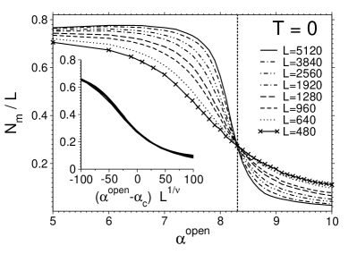
Figure 2: Results for the number $N_{m}$ of aligned letters (matches plus mismatches) as a function of gap opening penalty $\alpha^{\text{open}}$. Curves for different sequence lengths intersect at the critical parameter $\alpha_{c}$. For a more clear presentation, single data points are only shown for one system size. Inset: After rescaling the abscissa with appropriate values for $\alpha_{c}$ and $\nu$ the data listed in Tab. 1 collapses on a single master curve.

Fig. 2 displays $\left[\langle N_{m}\rangle_{T}\right]/L$ as a function of the gap open penalty $\alpha^{\text{open}}$ for different lengths $L$ and zero temperature. The curves for different sequence lengths intersect at the critical value $\alpha_{c}$ as expected for a second order phase transition. Using finite-size-scaling theory [26], we may extrapolate data from finite sequence lengths to the thermodynamic limit $L\rightarrow\infty$. In this limit the observable $\left[\langle N_{m}\rangle_{T}\right]/L$ is in the order of $1$ below the threshold, i.e. $\alpha^{\text{open}}<\alpha_{c}$, and it jumps to $0$ exactly at $\alpha_{c}$. In finite systems, $L<\infty$, the crossover extends over a range $\sim L^{-1/\nu}$ as can be seen in Fig. 2. Scaling theory leads us to expect that the behavior of $\left[\langle N_{m}\rangle_{T}\right](\alpha^{\text{open}};T;L)$ close to criticality is described by

$$\left[\langle N_{m}\rangle_{T}\right](\alpha^{\text{open}};T;L)/L=f\left((\alpha^{\text{open}}-\alpha_{c})L^{1/\nu}\right),$$ (7)

where $f$ is an universal scaling function and the exponent $\nu$ describes the divergence of the ”correlation length” at the critical point $\alpha^{\text{open}}=\alpha_{c}$. We used Eq. (7) to extract numerical values for the critical exponents $\nu$ and the critical gap costs $\alpha_{c}$ with high precession from all data for a fixed temperature simultaneously. The fit is performed by minimizing a weighted-$\chi^{2}$-like objective function $Q(\alpha_{c},\nu)$ [32], that measures the distance (in units of the standard error) of the data from the (a prior unknown) master curve. For the example in Fig. 2, i.e. $T=0$, we obtained $\alpha_{c}=8.306(4)$ and $\nu=1.58(5)$ with acceptable quality of $\hat{Q}\equiv Q(\alpha_{c},\nu)=2.2$ ($\hat{Q}$ should be in the order of $1$ [32]). Statistical errors have been determined by bootstrapping [33, 34]. Repeating this analysis for several temperatures one may probe the critical line $\alpha_{c}(T)$ (see below).

We also tested a related quantity, which is defined as the number of matches / mismatches plus the number of gaped letters $N_{m}+N_{g}$, which results in the same critical exponent and critical point within error bars (not shown). Gaps seem to play only a marginal role close to the critical point. We observe that the roughness $\Delta$ of the alignment path as defined above at the critical point diverges only logarithmically with the sequence length. This supports the equivalence the description of the description of both variants of the this quantity.

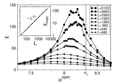
Figure 3: Critical fluctuations of $N_{m}$. The positions of the peaks approach the critical value $\alpha_{c}$ the and their heights diverge like $L^{\gamma/\nu}$. Inset: fit of $\chi_{\max}(L)$ to the scaling form $\sim L^{\gamma/\nu}$.

Next, we study the critical fluctuations of $N_{m}$. We define the susceptibility-like quantity $\chi=(\left[\langle N_{m}^{2}\rangle_{T}\right]-\left[\langle N_{m}\rangle_{T}\right]^{2})/L$ as a function of $\alpha^{\text{open}}$ (see Fig. 3).

Close to the critical point $\chi$ diverges like $\chi\sim L^{\gamma/\nu}$. In order to extract the height of the maxima from $\chi(\alpha^{\text{open}})$ we performed parabolic fits in the form $\chi(\alpha^{\text{open}})=-C(\alpha_{c}(L)-\alpha^{\text{open}})^{2}+\chi_{\max}(L)$ for each system size $L$. The exponent $\gamma$ itself is determined by a fit of $\chi_{\max}(L)$ to the scaling form $\sim L^{\gamma/\nu}$. For $T=0$, we obtain $\gamma/\nu=0.95(1)$.

One may also use the scaling of $\alpha_{c}(L)$ to determine the critical value $\alpha_{c}$ and the critical exponent $\nu$ as a cross check via $\alpha_{0}(L)=\alpha_{c}-AL^{-\nu}$. When restricting the range to $L\geq 1280$ we obtain $\nu=1.4(3)$ for $T=0$ which agrees within the error bars with the value stated above. Furthermore the critical value $\alpha_{c}$ agrees within 1.5 standard deviations. We also checked that those values agree for FTA, $T=1$.

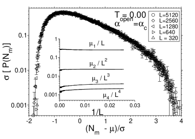
Figure 4: Rescaled distributions of the observable $N_{m}$ for $T=0$. Inset: scaling analysis of the moments. The first moment scales as $\mu_{1}\sim L$. Higher order moments increase slower than $\mu_{k}\sim L^{k}$.

Alternatively, one can determine $\gamma$ from the second moment of the averaged distribution $[P(N_{m})]$ of $N_{m}$ at $\alpha^{\text{open}}=\alpha_{c}$. Hence, we performed further simulations at criticality with a larger sample size (for the largest system size, $n^{\text{sample}}\approx 2\times 10^{4}$ for $T=0$ and $n^{\text{sample}}=1.6\times 10^{4}$ for $T>0$). This allowed us to cross check the value of $\gamma$ and to extract higher moments of the distribution.

Fig. 4 displays distributions $[P(\langle N_{m}\rangle_{T})]$ for $T=0$ (similar results have been obtained for $T>0$). The distributions have been rescaled to zero mean and unit variance. In all cases we observe that the first moments $\mu_{1}$ scale as $\mu_{1}\sim L^{1+\epsilon}$ with $\epsilon=0$ within the errorbars. For the second moment one would expect the scaling behavior $\mu_{2}\equiv L\chi\sim L^{1+\gamma/\nu}$. Indeed we find $\gamma/\nu=0.955(8)$ for OA by a least square fit. This is consistent with the numerical value obtained by the height of maxima. The third and the fourth moment scale as $\mu_{3}\sim L^{2+\gamma_{3}}$ and $\mu_{4}\sim L^{3+\gamma_{4}}$ respectively. For temperatures $T<2$ both exponents $\gamma_{3}$ and $\gamma_{4}$ agree within the statistical errors.

The resulting critical values $\alpha_{c}$ and critical exponents $\nu$, $\gamma$, $\gamma_{3}$,$\gamma_{4}$ are summarized in Tab. 1. All ratio of exponents, $\gamma/\nu$, $\gamma_{3}/\nu$ and $\gamma_{4}/\nu$, are in the order of $1$ and seem to increase with the temperature. Note that for a perfectly one-parameter scaling of the complete distribution with $\mu_{1}\sim L$ one would expect $\gamma/\nu=\gamma_{3}/\nu=\gamma_{4}/\nu=\ldots=1$. This property is only approximately fulfilled according to our data. This is shown in Fig. 5, where also the resulting phase diagram is displayed.

The standard order parameter in percolation problems is the relative size of the largest cluster. Since local sequence alignments (and its interpretation as DPRM) exhibits one spacial dimension, the observable $N_{m}/L$ can also be interpreted as order parameter, which is one if the alignment covers the entire sequences. The usual finite-size-scaling ansatz for the relative size of the largest cluster order parameter reads as

$$\left[\langle N_{m}\rangle_{T}\right](\alpha^{\text{open}};T;L)/L=L^{-\beta^{\text{geo}}/\nu}f\left((\alpha^{\text{open}}-\alpha_{c})L^{1/\nu}\right),$$ (8)

where the exponent $\beta^{\text{geo}}$ describes the divergence of the largest cluster. By comparing this relation with Eq. (7) we may infer $\beta^{\text{geo}}=0$ and verify that the scaling relation $\gamma+2\beta^{\text{geo}}=d\nu$ [26] (with $d=1$ in our case) is again only approximately fulfilled. We confirmed that $\beta=0$ within the errorbars by considering $\beta$ as free parameter in the finite-size-scaling analysis for $N_{m}$.

As mentioned above, the roughness only grows logarithmically with the system size. This implies that the fractal dimension $d_{r}$ of the alignment path equals the topological dimension $d=1$, which is in agreement with the scaling relation $d_{r}=d-\beta^{\text{geo}}/\nu$ in a trivial way.

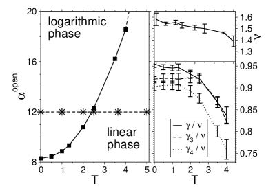
Figure 5: Results for FTA. Left: Phase diagram for FTA. The linear phase is located below the critical line. Right: critical exponents as a function of the temperature.

$T$		$\alpha_{c}$		$\nu$		$\gamma/\nu$		$\gamma_{3}/\nu$		$\gamma_{4}/\nu$
$0$.	$00$	$8$.	$306(4)$	$1$.	$58(5)$	$0$.	$955(8)$	$0$.	$920(5)$	$0$.	$903(9)$
$0$.	$50$	$8$.	$450(2)$	$1$.	$54(1)$	$0$.	$947(6)$	$0$.	$92(1)$	$0$.	$91(1)$
$1$.	$00$	$8$.	$871(4)$	$1$.	$55(2)$	$0$.	$946(6)$	$0$.	$92(1)$	$0$.	$91(1)$
$1$.	$33$	$9$.	$339(3)$	$1$.	$53(2)$	$0$.	$948(8)$	$0$.	$92(1)$	$0$.	$91(1)$
$2$.	$00$	$10$.	$791(3)$	$1$.	$51(2)$	$0$.	$931(9)$	$0$.	$92(1)$	$0$.	$89(1)$
$2$.	$50$	$12$.	$296(4)$	$1$.	$50(4)$	$0$.	$921(9)$	$0$.	$92(1)$	$0$.	$88(1)$
$3$.	$50$	$16$.	$227(1)$	$1$.	$46(1)$	$0$.	$87(1)$	$0$.	$870(8)$	$0$.	$80(1)$
$4$.	$00$	$18$.	$557(2)$	$1$.	$38(5)$	$0$.	$84(2)$	$0$.	$924(5)$	$0$.	$76(2)$

Table 1: Critical gap open penalty $\alpha_{c}$ and critical exponents $\nu$, $\gamma$, $\gamma_{3}$,$\gamma_{4}$ for the observable $N_{m}$.

III.2 Energetic properties

As mentioned above, the size of the largest cluster is usually regarded as the order parameter in percolation problems. In the non-percolating phase, the size of the largest cluster typically grows logarithmically with the system size whereas in the percolating phase its extension is comparable to the system size [26]. The average score of local alignments exhibits the same crossover when crossing the linear-logarithmic boundary. For this reason we regard the average score $\left[S\right]/L$ (OA), or free energy $\left[F_{T}\right]/L$ (FTA), per length as a second order parameter, as in [25]. Note that there is no direct geometrical interpretation for this quantity.

Scaling theory states that the order parameter scales as

$$\left[F_{T}\right]/L=L^{-\beta/\nu}f\left((\alpha-\alpha_{c})L^{1/\nu}\right)$$ (9)

with some universal scaling function $f$. This allows one to extract the critical value $\alpha_{c}$ and exponents $\nu$ and $\beta$ from the data with the same method as described above. Here, we fixed $\alpha_{c}$ and $\nu$ with the values that have been obtained from the data collapse for the observable $N_{m}$ and regard $\beta/\nu$ as a free parameter. The result for $T=0$ is shown in Fig. 6. The quality of these fits varied between $\hat{Q}=1.58$ for $T=1.00$ and $\hat{Q}=7.49$ for $T=4.00$.

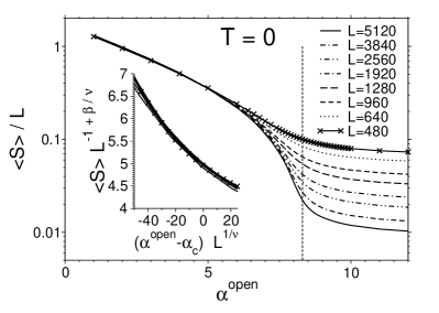
Figure 6: Finite-size-scaling analysis for the average score per length.

By regarding $\nu$ and $\beta$ as free parameters, we also used the scaling form Eq. (9) as a second cross check for the exponent $\nu$. Within the error bars it is comparable with the results of the finite-size-scaling analysis for the observable $N_{m}$ (for example $\nu=1.50(7)$ for $T=0$). For larger temperatures ($T\geq 2$) only system sizes $L\geq 1280$ led to convincing results for this kind of check.

$T$		$\beta/\nu$		$\omega$
$0$.	$00$	$0$.	$6324(07)$	$0$.	$386(5)$
$0$.	$50$	$0$.	$6406(10)$	$0$.	$391(5)$
$1$.	$00$	$0$.	$6443(11)$	$0$.	$387(6)$
$1$.	$33$	$0$.	$6564(09)$	$0$.	$380(9)$
$2$.	$00$	$0$.	$6835(10)$	$0$.	$36(1)$
$2$.	$50$	$0$.	$7081(08)$	$0$.	$33(1)$
$3$.	$50$	$0$.	$7691(06)$	$0$.	$23(2)$
$4$.	$00$	$0$.	$7958(05)$	$0$.	$20(2)$

Table 2: Critical exponents for the average score / free energy per length. $\beta/\nu$ was obtained from finite-size scaling (see Fig. 6) and cross checked via the scaling of the first moment of the score distribution at criticality $\alpha=\alpha_{c}$. The exponent $\omega$ describe the fluctuations of the score distribution at $\alpha=\alpha_{c}$.

As can be seen in the second column of table Tab. 2, the free energy per length $\left[F_{T}\right]/L$ decreases like $\sim L^{-\beta/\nu}$, where $\beta/\nu$ increases monotonously with the temperature from $0.6324(7)$ to $0.7958(5)$. For small temperatures, i.e. $T<2$, the exponent $\beta\approx 1$ is not temperature dependent. Hence the phase behavior regarding the exponent $\beta$ is not universal any more when exceeding $T=2$.

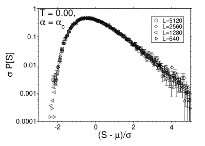
Figure 7: Rescaled score distributions $T=0$. The free-energy distributions of FTA look comparable.

III.3 Free-energy distributions close to criticality

In analogy to the distribution of the observable $N_{m}$ in Fig. 4, the resulting rescaled score distributions right at $\alpha^{\text{open}}=\alpha_{c}$ are shown in Fig. 7. Simulations for FTA yield comparable results. We performed an analysis of the moments of $P[S]$ and $P[F]$ respectively. The first moment scales as $\mu_{1}\sim L^{1-\beta/\nu}$ as expected from the finite-size analysis shown in Fig. 6. We checked that the fit parameters agree with those from finite-size scaling.

Regarding the second moment, no divergence was observed. Its scaling behavior is given by $\mu_{2}\sim L^{1-\omega}$ with $\omega>0$. The resulting fit parameters are listed in Tab. 2. In the limit $\alpha^{\text{open}}\rightarrow\infty$ and $L\rightarrow\infty$, the score distribution is predicted to follow a Gumbel distribution

$$P_{\text{gumbel}}(S)=\lambda\exp\left[-\lambda(S-S_{0})-\exp(-\lambda(S-S_{0}))\right]$$ (10)

(according to the Karlin-Altschul-Dembo theory [35, 36, 37]).

In the linear phase the conditions of this theory are not valid any more. Interestingly, right at the critical point, the shape of the distributions are well described by a Gumbel distribution, at least in the high probability region (down to $P[S]\sim 10^{-4}$). In previous studies we observed parabolic corrections to Eq. (10) that occur in the far right tail of the optimal score distribution [39, 38]. The corrected distribution is empirically well described by

$$P(S)=\frac{1}{z^{\prime}}P_{\text{gumbel}}(S)\exp\left[-\lambda_{2}(S-S_{0})^{2}\right],$$ (11)

where $\lambda_{2}$ is a correction parameter and the normalization constant $z^{\prime}$ is indistinguishable from $1$. We found evidence that $\lambda_{2}$ vanishes for $L\rightarrow\infty$ but persists even for gapless alignment $\alpha^{\text{open}}=\infty$ [38].

Here, we extend this study to finite-temperature alignment, i.e. to the free-energy distribution as a generalization of the score distribution. We employed generalized ensemble Monte-Carlo simulations combined with Wang-Landau sampling [40] in the sequence space (details can be found elsewhere [41]). The (production) run for $L=120$ employed $4.8\times 10^{7}$ Monte Carlo steps for each distribution over the disorder.

In the following, we use the phase diagram as a guide to study the free-energy distribution for various temperatures. We kept the gap-costs fixed ($\alpha^{\text{open}}=12$, $\beta^{\text{ext}}=1$) and only varied the temperature (between $T=0$ and $T=5$). The interpolating points are indicated by stars in the phase diagram in Fig. 5.

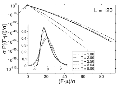
Figure 8: Rescaled free-energy distribution of finite-temperature alignments. At $T=2.50$ and below, the data is well described by a modified Gumbel distribution. For large temperatures an exponential tail is observed.
Inset: The same data shown with a linear ordinate. In the high probability region the data for $T=5.00$ is well described by a Gaussian distribution.

$T$		$\lambda$		$10^{4}\lambda_{2}$		$s_{0}$
$0$.	$00$	$0$.	$2966(4)$	$3$.	$182(1)$	$37$.	$4(1)$
$1$.	$00$	$0$.	$2924(1)$	$2$.	$900(5)$	$24$.	$6(1)$
$2$.	$00$	$0$.	$2907(2)$	$3$.	$122(7)$	$31$.	$56(6)$
$2$.	$50$	$0$.	$2980(2)$	$3$.	$16(1)$	$38$.	$29(7)$

Table 3: Fit parameters of least $\chi^{2}$-fits of the free-energy distributions to the modified Gumbel distribution Eq. (11) for $L=120$ in the logarithmic phase.

In the logarithmic regime ($T=0,1,2,2.5$) the free-energy distribution is well described by the modified Gumbel distribution Eq. (11) (see Fig. 8). Note that we have again rescaled the distributions to unit variance and zero mean. The fit parameters only change slightly with the temperature (see Tab. 3).

The crossover from the logarithmic to the linear regime comes along with a change of the skewness, as can be seen in the inset of Fig. 8. In the high probability region, for a large value $T=5.00$, a Gaussian distribution describes the data well. This was confirmed by a Kolmogorov-Smirnov test that yielded a p-value of $0.14$. For $T=1/0.275\approx 3.64$ the evidence for a Gaussian distribution is much smaller (a p-value of $2\times 10^{-11}$). We also checked that the change of the shape is accompanied by a change from logarithmic to linear growth of typical free energies (the position of the maximum) with the sequence length, i.e. the free energy becomes extensive (not shown here). This result can be understood in the following way: The partition functions that appears in the transfer matrix calculation Eq. (II) become (more or less) independent and hence factorize in the linear phase. The total free energy decomposes into a sum of independent contributions and the central limit theorem applies.

When considering the rare-event tail at higher temperatures, the free-energy distribution is rather exponential than Gaussian, as can be seen in the main plot of Fig. 8. Hence, we observe a crossover from a Gaussian distribution in the high probability region to the characteristic exponential tail of the Gumbel distribution. With the same argumentation as for the optimal alignment, sequence pairs appearing in the tail feature high similarities. The overall free energy is dominated by the ground state. This was confirmed by looking at the difference between the free energy and the ground-state energy for those sequences that occur in the tail of the distribution. The summation in the transfer matrix are virtually replaced by maximization yielding an exponential tail. The finite-size effect, that is responsible for the curvature of the optimal alignment statistics seems to be of marginal order in this case.

IV Summary

We presented a finite-size-scaling analysis of the linear-logarithmic phase transition of finite-temperature protein sequence alignment. This phase transition is crucial to determine the set of parameters where the alignment is of highest sensitivity. We have used the blosum62 scoring matrix together with affine gap costs, which is the most frequently used scoring system for actual database queries. This goes much beyond previous studies, which have investigated only simple scoring systems.

Two order parameters were studied in detail: the number of matches (i.e. the alignment length) and the average free energy per length. We have analyzed the phase transition using finite-size scaling techniques. Using sophisticated algorithms, large systems could be studied, such that corrections to finite-size scaling are negligible. The resulting critical line $a_{c}(T)$ in the range $T=0\ldots 4$ provides a guide for biological applications where suboptimal alignments play an important role.

Numerical values of the critical exponents $\nu$, $\gamma$ and $\beta$ suggest that the percolation transition is not universal with respect to different temperature values.

The free-energy distribution, which can be seen as a generalization of the score distribution over random sequences, crosses over from a modified Gumbel distribution with a parabolic correction in the tail given by Eq. (11) in the logarithmic phase to a modified Gaussian distribution with a linear rare-event tail in the linear phase. This is another example showing that the large-deviation properties of order-parameter distributions change significantly close to phase transitions.

References

- [1] A. Krogh R. Durbin, S. Eddy and G. Mitchison. Biological Sequence Analysis. Cambridge University Press, 1998.
- [2] P. Clote and R. Backofen. Computational Molecular Biology: An Introduction. John Wiley & Sons, Ltd., 2005.
- [3] S.F. Altschul, W. Gish, W. Miller, E.W. Myers, and D.J. Lipman. Basic Local Alignment Search Tool. J. Mol. Biol., 215:403–410, 1990.
- [4] W. R. Pearson and D. J. Lipman. Improved tools for biological sequence comparison. PNAS USA, 85(8):2444, 1988.
- [5] T. F. Smith and M. S. Waterman. Identification of Common Molecular Subsequences. J. Mol. Biol., 147:195–197, 1981.
- [6] M.Q. Zhang and T.G. Marr. Alignment of Molecular Sequences Seen as Random Path Analysis. J. Theor.Biol., 174:119, 1995.
- [7] D. A. Huse and C. L. Henley. Pinning and Roughening of Domain Walls in Ising Systems Due to Random Impurities. Phys. Rev. Lett., 54(25):2708, 1985.
- [8] M. Kardar. Replica Bethe ansatz studies of two-dimensional interfaces with quenched random impurities. Nucl. Phys. B, 290:582, 1987.
- [9] M. Mezard. On the glassy nature of random directed polymers in two dimensions. J. Physique France, 51:1831, 1990.
- [10] D. S. Fisher and D. A. Huse. Directed paths in a random potential. Phys. Rev. B, 43(13):10728, 1991.
- [11] M. Kardar. Directed paths in random media. In F. David, P. Ginzparg, and J. Zinn-Justin, editors, Fluctuating Geometries in Statistical Mechanics and Field Theory: Les Houches Summer School, Session LXII, 2 August - 9 September 1994, 1994.
- [12] U. Mückstein, I.L. Hofacker, and P.F. Stadler. Stochastic pairwise alignments. Bioinformatics, 18(2):153, 2002.
- [13] L. Jaroszewski, W. Li, and A. Godzik. In search for more accurate alignments in the twilight zone. Protein Sci, 11(7):1702, 2002.
- [14] R. Koike, K. Kinoshita, and A. Kidera. Probabilistic description of protein alignments for sequences and structures. Proteins, 56(1):157, 2004.
- [15] R. Koike, K. Kinoshita, and A. Kidera. Probabilistic alignment detects remote homology in a pair of protein sequences without homologous sequence information. Proteins, 66(3):655, 2007.
- [16] S. Miyazawa. A reliable sequence alignment method based on probabilities of residue correspondences. Protein Eng., 8(10):999, 1995.
- [17] M. Kschischo and M. Lässig. Finite-temperature sequence alignment. In Pacific Symposium on Biocomputing 5, 2000.
- [18] R. Olsen, R. Bundschuh, and T. Hwa. Rapid Assessment of Extremal Statistics for Local Alignment with Gaps. In T. Lengauer, R. Schneider, P. Bork, D. Brutlag, J. Glasgow, H.-W. Mewes, and R. Zimmer, editors, Proceedings of the seventh International Conference on Intelligent Systems for Molecular Biology, volume 270, page 211, Menlo Park, CA, 1999. AAAI Press.
- [19] D. Drasdo, T. Hwa, and M. Lässig. Scaling Laws and Similarity Detection in Sequence Alignment with Gaps. J. Comp. Biol., 7:115–141, 2000.
- [20] M. S. Waterman and M. Eggert. A new algorithm for best subsequence alignments with application to tRNA-rRNA comparisons. J. Mol. Biol., 197(4):723, 1987.
- [21] R. Arratia and M.S. Waterman. A Phase Transition for the Score in Matching Random Sequences Allowing Deletions. Ann.Appl. Prob., 4:200, 1994.
- [22] R. Bundschuh and T. Hwa. An analytic study of the phase transition line in local sequence alignment with gaps. Discr. Appl. Math., 104(1-3):113, 2000.
- [23] M. Vingron and M. S. Waterman. Sequence alignment and penalty choice: Review of concepts, case studies and implications. J. Mol. Biol., 235(1):1, 1994.
- [24] T. Hwa and M. Lässig. Optimal Detection of Sequence Similarity by Local Alignment. In S. Istrail, P. Pevzner, and M.S. Waterman, editors, Proceedings of the Second Annual International Conference on Computational Molecular Biology (RECOMB98), page 109, 1998.
- [25] M.E. Sardiu and G. Alves and Y. Yu. Score statistics of global sequence alignment from the energy distribution of a modified directed polymer and directed percolation problem. Phys.Rev.E., 72:061917, 2005.
- [26] D. Stauffer and A. Aharony. Introduction To Percolation Theory. CRC, 1994.
- [27] S. Heinkoff and J.G. Heinkoff. Amino acid substitution matrices from protein blocks. PNAS USA, 89:10915–10919, 1992.
- [28] O. Gotoh. An improved algorithm for matching biological sequences. J. Mol. Biol., 162:705, 1982.
- [29] G.H. Gonnet, M.A. Cohen, and S.A. Benner. Exhaustive matching of the entire protein sequence database. Science, 256(5062):1443, 1992.
- [30] X. Gu and W.-H. Li. The size distribution of insertions and deletions in human and rodent pseudogenes suggests the logarithmic gap penalty for sequence alignment. J. Mol. Evol., 40(4):464, 1995.
- [31] R. Cartwright. Logarithmic gap costs decrease alignment accuracy. BMC Bioinformatics, 7(1):527, 2006.
- [32] J. Houdayer and A. K. Hartmann. Low-temperature behavior of two-dimensional Gaussian Ising spin glasses. Phys. Rev. B, 70:014418, 2004.
- [33] B. Efron. Bootstrap Methods: Another look at the Jackknife. Ann. Stat., 7:1, 1979.
- [34] A.K. Hartmann. Practical Guide to Computer Simulations. World Scientific, Singapore, 2009.
- [35] S. Karlin and S. F. Altschul. Methods for assessing the statistical significance of molecular sequence features by using general scoring schemes. PNAS USA, 87(6):2264, 1990.
- [36] S. Karlin and A. Dembo. Limit Distributions of Maximal Segmental Score among Markov-Dependent Partial Sums. Adv. Appl. Prob., 24:113, 1992.
- [37] A. Dembo, S. Karlin, and O. Zeitouni. Limit Distribution of Maximal Non-Aligned Two-Sequence Segmental Score. Ann. Prob., 22:2022–2039, 1994.
- [38] Wolfsheimer, S. and Burghardt, B. and Hartmann, A. K. Local sequence alignments statistics: deviations from Gumbel statistics in the rare-event tail. Algor. Mol. Biol., 2(1):9, 2007.
- [39] A.K. Hartmann. Sampling rare events: Statistics of local sequence alignments. Phys. Rev. E, 65:056102, 2002.
- [40] F. G. Wang and D. P. Landau. Efficient, multiple-range random walk algorithm to calculate the density of states. Phys. Rev. Lett., 86:2050, 2001.
- [41] S. Wolfsheimer, I. Herms, S. Rahmann, and A. K. Hartmann. Accurate Statistics for Local Sequence Alignment with Position-Dependent Scoring by Rare-Event Sampling. submitted.